Cell-Free Massive MIMO Surveillance of Multiple Untrusted Communication Links

Abstract

A cell-free massive multiple-input multiple-output (CF-mMIMO) system is considered for enhancing the monitoring performance of wireless surveillance, where a large number of distributed multi-antenna aided legitimate monitoring nodes (MNs) proactively monitor multiple distributed untrusted communication links. We consider two types of MNs whose task is to either observe the untrusted transmitters or jam the untrusted receivers. We first analyze the performance of CF-mMIMO surveillance relying on both maximum ratio (MR) and partial zero-forcing (PZF) combining schemes and derive closed-form expressions for the monitoring success probability (MSP) of the MNs. We then propose a joint optimization technique that designs the MN mode assignment, power control, and MN-weighting coefficient control to enhance the MSP based on the long-term statistical channel state information knowledge. This challenging problem is effectively transformed into tractable forms and efficient algorithms are proposed for solving them. Numerical results show that our proposed CF-mMIMO surveillance system considerably improves the monitoring performance with respect to a full-duplex co-located massive MIMO proactive monitoring system. More particularly, when the untrusted pairs are distributed over a wide area and use the MR combining, the proposed solution provides nearly a thirty-fold improvement in the minimum MSP over the co-located massive MIMO baseline, and forty-fold improvement, when the PZF combining is employed.

I Introduction

The widespread use of mobile devices along with the explosive popularity of wireless data services offered by fifth generation (5G) networks has led to the emergence of the so-called infrastructure-free communication systems, which include device-to-device (D2D), aerial vehicle (UAV)-aided communications, internet and so on. Although these wireless transmission systems provide an efficient and convenient means for establishing direct connections between mobile terminals, unauthorised or malicious users may misuse these networks to perform illegal activities, commit cyber crime, and jeopardize public safety. As a remedy, legitimate monitoring has attracted considerable attention in recent years [2].

In contrast to wireless physical-layer security (PLS), which aims for making the transmitted information indecipherable to illegitimate monitors [3], this line of PLS puts emphasis on legally monitoring the communications of an untrusted pair. Wireless surveillance is typically classified into three main paradigms based on the kind of strategies used in the surveillance process by a legitimate monitor: $1)$ passive monitoring [4], $2)$ proactive monitoring [4], and $3)$ spoofing relaying [5]. In passive monitoring, the legitimate monitor silently observes an untrusted link and, hence, successful monitoring can only be achieved for the scenarios where the strength of the monitoring link is better than that of the untrusted one. In proactive monitoring, the legitimate monitor operates in a full-duplex (FD) mode, simultaneously observing the untrusted link and sending a jamming signal to interfere with the reception of the untrusted receiver (UR), thereby degrading the rate of the untrusted link. This improves the monitoring success probability (MSP) [6], which is one of the fundamental monitoring performance objectives. Finally, in the context of spoofing relaying, the FD monitor observes the untrusted link and alters the channel information sent over the untrusted link to adjust its rate requirement.

TABLE I: Explicitly Contrasting Our Contributions to the Literature

Feature	[7]	[8]	[9]	[10]	[11]	[12]	[13]	[14]	our work
Multiple untrusted pairs		✓	✓	✓a	✓	✓			✓
Multiple monitors						✓b	✓	✓b	✓
Multiple-antenna technique	✓			✓					✓
Statistical CSI	$\checkmark$								✓
Coherent monitoring									✓
Distributed									✓

• ^a Two untrusted pairs, ^b two monitors.

Since the publication of the pioneering paper [4], proactive monitoring has been widely studied under diverse untrusted communication scenarios, such as multiple-input multiple-output (MIMO) systems [6, 15, 16, 7], relaying systems [5, 17, 18, 19], UAV networks [20, 21], cognitive radio networks [22, 23], and intelligent reflecting surface (IRS)-aided surveillance systems [24, 25]. Specifically, in [6, 15], multi-antenna techniques were utilized to improve the monitoring performance. In [6], an optimization framework was developed for the jamming power control and transmit/receive beamforming vectors at the legitimate monitor by maximizing the MSP. The authors of [15] established an optimization framework for joint precoding design and jamming power control, by taking into account the impact of jamming on the performance of other legitimate users. Low-complexity suboptimal zero-forcing (ZF)-based beamforming schemes were also proposed in [15]. Under the more practical assumption of imperfect channel state information (CSI), the maximization of the worst-case MSP attained by multi-antenna aided proactive monitoring systems was investigated in [16], where the CSI error was deterministically bounded. Additionally, by assuming the knowledge of the imperfect instantaneous CSI of the observing link and CSI statistics of the jamming and the untrusted links, Zhang et al. [7] studied the performance of multi-antenna assisted proactive monitoring in uplink systems and derived semi-closed-form expressions for both the MSP and monitoring rate. Proactive monitoring was investigated in [5] in dual-hop decode-and-forward relaying systems, where the legitimate monitor can adaptively act as a monitor, a jammer or a helper, while proactive monitoring was studied in [17] via jamming designed for amplify-and-forward relay networks. Moon et al. [18] extended the results of [17] to multi-antenna aided multi-relay systems. Later, UAV-aided information surveillance was proposed in [20], where an FD ground monitor observes the untrusted link and simultaneously sends the collected untrusted information to the UAV. By contrast, Li et al. [21] relied on a legitimate UAV to track untrusted UAV-to-UAV communications and developed both an energy-efficient jamming strategy and a tracking algorithm. The proactive monitoring concept of cognitive systems was introduced in [22] and [23], where the secondary users are allocated to share the spectrum of the untrusted users, provided that they are willing to act as an observer or friendly jammer monitoring the untrusted link. Recently, IRSs have also found their way into information surveillance systems, where the IRS is used for degrading the untrusted channel’s rate [24] and for improving the observing channel [25] to further enhance the monitoring performance. Finally, beneficial IRS deployment strategies and joint beamforming design problems were proposed in [25].

I-A Knowledge Gap and Motivations

It is important to point out that most studies tend to investigate simple setups concerning the untrusted communication links and/or observing links. More specifically, a popular assumption in the aforementioned literature is that there is a single untrusted link. This assumption is optimistic, because realistic systems are likely to have more than one untrusted communication links in practice. In this context, Xu and Zhu [8] have studied proactive monitoring using a single monitor for observing multiple untrusted pairs in scenarios associated with either average rate or with outage probability constrained untrusted links. Li et al. [9] used proactive monitoring with relaying features to increase the signal-to-interference-plus-noise ratio (SINR) of multiple untrusted links, which results in a higher rate for the untrusted links, and hence, higher observation rate. Moreover, Zhang et al. in [10] characterized the achievable monitoring rate region of a single-monitor surveillance system observing two untrusted pairs operating within the same spectral band and using a minimum-mean-squared-error successive interference cancellation (MMSE-SIC) receiver. Proactive monitoring was studied in [11] for the downlink of an untrusted non-orthogonal multiple access (NOMA) network with one untrusted transmitter (UT) and multiple groups of URs, while relying on a single-antenna monitor equipped with a SIC receiver.

In the case of a distributed deployment of untrusted pairs over a geographically wide area, it is impractical to cater for the direct monitoring of each and every untrusted pair by relying on a single monitor. Hence, attaining a given target MSP performance for the untrusted pairs is a fundamental challenge. Therefore, cooperative operation relying on a single primary FD monitor and an auxiliary assistant FD monitor supervising a single UT and multiple URs was proposed in [12] for maximizing the monitoring energy efficiency via optimizing the jamming power and the cooperation strategy selected from a set of four specific strategies. Later, Moon et al. [13] looked into proactive monitoring relying on a group of single-antenna aided intermediate relay nodes harnessed for supporting a legitimate monitor, which acts either as a jammer or as an observer node. Furthermore, the authors of [14] harnessed a pair of single-antenna half-duplex nodes that take turns in performing observing and jamming. However, the significant drawback of these studies is that they only focused on either the single-untrusted-link scenario [13, 14] or on a specific system setup [12]. Another main concern is the overly optimistic assumption of knowing instantaneous CSI of all links at the monitor nodes. In this case, the system level designs must be re-calculated on the small-scale fading time scale, which fluctuates quickly in both time and frequency. Therefore, the study of how to efficiently carry out surveillance operation using multiple monitors in the presence of multiple untrusted pairs is extremely timely and important, yet, this is still an open problem at the time of writing.

To address the need for reliable information surveillance in complex practical scenarios, we are inspired by the emerging technique of cell-free massive MIMO (CF-mMIMO) [26] to propose a new proactive monitoring system, termed as CF-mMIMO surveillance. CF-mMIMO constitutes an upscaled version of user-centric network MIMO. In contrast to traditional cellular systems, i) fixed cells and cell boundaries disappear in CF-mMIMO and ii) the users are served coherently by all serving antennas within the same time-frequency resources [27]. Therefore, CF-mMIMO offers significantly higher degrees of freedom in managing interference, hence resulting in substantial performance improvements for all the users over conventional cellular networks. The beneficial features of CF-mMIMO are its substantial macro diversity, favorable propagation, and ubiquitous coverage for all users in addition to excellent geographical load-balancing. Owing to these eminent advantages, CF-mMIMO has sparked considerable research interest in recent years and has yielded huge performance gains in terms of spectral efficiency (SE) [26, 28], energy efficiency [29, 30], and security [31, 32]. More interestingly, recent research has shown that utilizing efficient power allocation and receive combining/transmit precoding designs in CF-mMIMO, relying on multiple-antenna access points (APs) further enhances the system performance [33, 34].

Our CF-mMIMO information surveillance system is comprised of a large number of spatially distributed legitimate multiple-antenna monitoring nodes (MNs), which jointly and coherently perform surveillance of multiple untrusted pairs distributed over a wide geographic area. In our system, there are typically several MNs in each other’s close proximity for any given untrusted pair. Thus, high macro-diversity gain and low path loss can be achieved, enhancing the observing channel rates and degrading the performance of untrusted links. Therefore, CF-mMIMO surveillance is expected to offer an improved and uniform monitoring performance for all the untrusted pairs compared to its single-monitor (co-located) massive MIMO based counterpart. In addition, the favorable propagation characteristics of CF-mMIMO systems allow our CF-mMIMO surveillance system to employ simple processing techniques, such as linear precoding and combining, while still delivering excellent monitoring performance. More importantly, when the CF-mMIMO concept becomes integrated into our wireless surveillance system, a virtual FD mode can be emulated, despite relying on half-duplex MNs. Relying on half-duplex MNs rather than FD MNs, makes the monitoring system more cost-effective and less sensitive to residual self interference. More particularly, two types of MNs are considered: 1) a specifically selected subset of the MNs is purely used for observing the UTs; 2) the rest of the MNs cooperatively jam the URs. In addition, since the MNs are now distributed across a large area, the inter-MN interference encountered is significantly reduced compared to a conventional FD monitoring/jamming system. Moreover, harnessing the channel hardening attributes of CF-mMIMO systems enables us to dynamically adjust the observing vs. jamming mode, the MN transmit power, and the MN-weighting coefficients for maximizing the overall monitoring performance based on only long-term CSI. Table I boldly and explicitly contrasts our contributions and benchmarks them against the state-of-the art. We further elaborate on the novel contributions of this work in the next subsection in a point-wise fashion.

I-B Key Contributions

The main technical contributions and key novelty of this paper are summarized as follows:

• We propose a novel wireless surveillance system, which is based on the CF-mMIMO concept relying on either observing or jamming mode assignment. In particular, by assuming realistic imperfect CSI knowledge, we derive exact closed-form expressions for the MSP of CF-mMIMO surveillance system with multiple-antenna MNs over multiple untrusted pairs for distributed maximum ratio (MR) and partial ZF (PZF) combining schemes. Additionally, we show that when the number of MNs in observing mode tends to infinity, the effects of inter-untrusted user interference, inter-MN interference, and noise gradually disappear. Furthermore, when the number $M_{\mathtt{J}}$ of MNs in the jamming mode goes to infinity, we can reduce the transmit power of each MN by a factor of $\frac{1}{M_{\mathtt{J}}}$ while maintaining the given SINR.

• We formulate a joint optimization problem for the MN mode assignment, power control, and MN-weighting coefficient control for maximizing the minimum MSP of all the untrusted pairs subject to a per-MN average transmit power constraint. We solve the minimum MSP maximization problem by casting the original problem into three sub-problems, which are solved using an iterative algorithm.

• We also propose a greedy UT grouping algorithm for our CF-mMIMO system relying on PZF combining scheme. Our numerical results show that the proposed joint optimization approach significantly outperforms the random mode assignment, equal power allocation, and equal MN-weighting coefficient based approaches. The simulation results also confirm that, compared to the co-located massive MIMO aided proactive monitoring system relying on FD operation, where all MNs are co-located as an antenna array and simultaneously perform observation and jamming, our CF-mMIMO surveillance system brings the MNs geographically closer to the untrusted pairs. Thus leads to a uniformly good monitoring performance for all untrusted pairs.

Notation: We use bold upper case letters to denote matrices, and lower case letters to denote vectors. The superscripts $(\cdot)^{*}$, $(\cdot)^{T}$, and $(\cdot)^{\dagger}$ stand for the conjugate, transpose, and conjugate-transpose (Hermitian), respectively. A zero-mean circular symmetric complex Gaussian distribution having a variance of $\sigma^{2}$ is denoted by $\mathcal{CN}(0,\sigma^{2})$, while $\mathbf{I}_{N}$ denotes the $N\times N$ identity matrix. Finally, $\mathbb{E}\{\cdot\}$ denotes the statistical expectation.

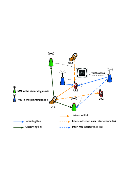
Figure 1: CF-mMIMO surveillance system model with the assigned MNs in observing mode and jamming mode along with the received desired and interference signals at a typical untrusted pair (UT $1$ and UR $1$).

II System Model

In this section, we introduce the CF-mMIMO surveillance system model for two different combining schemes. As shown in Fig. 1, we consider a surveillance scenario, where $M$ MNs are employed to monitor $K$ untrusted communication pairs. Let us denote the sets of MNs and untrusted communication pairs by $\operatorname{\mathcal{M}}\triangleq\{1,\dots,M\}$ and $\operatorname{\mathcal{K}}\triangleq\{1,\dots,K\}$, respectively. Each UT and UR is equipped with a single antenna, while each MN is equipped with $N$ antennas. All MNs, UTs, and URs are half-duplex devices. We assume that all MNs are connected to the central processing unit (CPU) via fronthaul links. The MNs can switch between observing mode, where they receive untrusted messages, and jamming mode, where they send jamming signals to the URs. The assignment of each mode to its corresponding MN is designed to maximize the minimum MSP over all the untrusted links, as it will be discussed in Section IV. We use the binary variable $a_{m}$ to show the mode assignment for each MN $m$, so that

$$a_{m}\triangleq\begin{cases}1,&\text{if MN $m$ operates in the jamming mode,}\\ 0,&\mbox{if MN $m$ operates in the observing mode}.\end{cases}$$ (1)

Note that we consider block fading channels, where the fading envelope of each link stays constant during the transmission of a block of symbols and changes to an independent value in the next block. The jamming channel (observing channel) vector between the $m$-th MN and the $k$-th UR ($k$-th UT) is denoted by ${\bf g}_{mk}^{\mathtt{J}}\in\mathbb{C}^{N\times 1}$ (${\bf g}_{mk}^{\mathtt{O}}\in\mathbb{C}^{N\times 1}$), $\forall k\in\operatorname{\mathcal{K}},m\in\operatorname{\mathcal{M}}$, respectively. It is modelled as ${\bf g}_{mk}^{\mathtt{J}}=\sqrt{\beta_{mk}^{\mathtt{J}}}\tilde{{\bf g}}_{mk}^{\mathtt{J}},~{}({\bf g}_{mk}^{\mathtt{O}}=\sqrt{\beta_{mk}^{\mathtt{O}}}\tilde{{\bf g}}_{mk}^{\mathtt{O}})$, where $\beta_{mk}^{\mathtt{J}}$ ($\beta_{mk}^{\mathtt{O}}$) is the large-scale fading coefficient and $\tilde{{\bf g}}_{mk}^{\mathtt{J}}\in\mathbb{C}^{N\times 1}$ ($\tilde{{\bf g}}_{mk}^{\mathtt{O}}\in\mathbb{C}^{N\times 1}$) is the small-scale fading vector containing independent and identically distributed (i.i.d.) $\mathcal{CN}(0,1)$ random variables (RVs). Furthermore, the channel gain between the $\ell$-th UT and the $k$-th UR is $h_{\ell k}=(\beta_{\ell k}^{\mathtt{U}})^{1/2}\breve{h}_{\ell k}$, where $\beta_{\ell k}^{\mathtt{U}}$ is the large-scale fading coefficient and $\breve{h}_{\ell k}$ represents small-scale fading, distributed as $\mathcal{CN}(0,1)$. We note that $h_{kk}$ models the channel coefficient of the $k$-th untrusted link spanning from the $k$-th UT to the $k$-th UR, $\forall k\in\operatorname{\mathcal{K}}$. Finally, the channel matrix between MN $m$ and MN $i$, $\forall m,i\in\operatorname{\mathcal{M}}$, is denoted by ${\bf F}_{mi}\in\mathbb{C}^{N\times N}$ where its elements, for $i\neq m$, are i.i.d. $\mathcal{CN}(0,\beta_{mi})$ RVs and $\operatorname{\mathbf{F}}_{mm}=\mathbb{0},\forall m$. Note that the channels ${\bf g}_{mk}^{\mathtt{J}}$ and ${\bf g}_{mk}^{\mathtt{O}}$ may be estimated at the legitimate MN by overhearing the pilot signals sent by UT $k$ and UR $k$, respectively [18]. By following [26], for the minimum-mean-square-error (MMSE) estimation technique and the assumption of orthogonal pilot sequences, the estimates of ${\bf g}_{mk}^{\mathtt{J}}$ and ${\bf g}_{mk}^{\mathtt{O}}$ can be written as $\hat{{\bf g}}_{mk}^{\mathtt{J}}\sim\mathcal{CN}(\mathbb{0},\gamma_{mk}^{\mathtt{J}}\mathbf{I}_{N})$ and $\hat{{\bf g}}_{mk}^{\mathtt{O}}\sim\mathcal{CN}(\mathbb{0},\gamma_{mk}^{\mathtt{O}}\mathbf{I}_{N})$, respectively, where $\gamma_{mk}^{\mathtt{J}}=\frac{\tau_{\mathrm{t}}\rho_{\mathrm{t}}(\beta_{mk}^{\mathtt{J}})^{2}}{\tau_{\mathrm{t}}\rho_{\mathrm{t}}\beta_{mk}^{\mathtt{J}}+1}$ and $\gamma_{mk}^{\mathtt{O}}=\frac{\tau_{\mathrm{t}}\rho_{\mathrm{t}}(\beta_{mk}^{\mathtt{O}})^{2}}{\tau_{\mathrm{t}}\rho_{\mathrm{t}}\beta_{mk}^{\mathtt{O}}+1}$ with $\rho_{\mathrm{t}}$ and $\tau_{\mathrm{t}}\geq 2K$ being the normalized transmit power of each pilot symbol and the length of pilot sequences, respectively. Since it is difficult (if not impossible) for the legitimate MNs to obtain the CSI of untrusted links, we assume that $h_{k\ell}$ is unknown to the MNs.

All the UTs simultaneously send independent untrusted messages to their corresponding URs over the same frequency band. The signal transmitted from UT $k$ is denoted by $x_{k}^{\mathtt{O}}=\sqrt{\rho_{\mathtt{UT}}}s_{k}^{\mathtt{O}}$, where $s_{k}^{\mathtt{O}}$, with $\mathbb{E}\left\{|s_{k}^{\mathtt{O}}|^{2}\right\}=1$, and $\rho_{\mathtt{UT}}$ represent the transmitted symbol and the normalized transmit power at each UT, respectively. At the same time, the MNs in jamming mode intentionally send jamming signals to interrupt the communication links between untrusted pairs. This enforces the reduction of the achievable data rate at the URs, thereby enhancing the MSP. More specifically, the MNs operating in jamming mode use the MR transmission technique, also known as conjugate beamforming, in order to jam the reception of the URs. Note that MR is considered because it maximizes the strength of the jamming signals at the URs. Let us denote the jamming symbol intended for the untrusted link $k$ by $s_{k}^{\mathtt{J}}$, which is a RV with zero mean and unit variance. When using MR precoding, the $N\times 1$ signal vector transmitted by MN $m$ can be expressed as

$${\bf x}_{m}^{\mathtt{J}}=a_{m}\sqrt{\rho_{\mathtt{J}}}\sum_{k\in\mathcal{K}}\sqrt{\theta_{mk}}\left(\hat{{\bf g}}_{mk}^{\mathtt{J}}\right)^{*}s_{k}^{\mathtt{J}},$$ (2)

where $\rho_{\mathtt{J}}$ is the maximum normalized transmit power at each MN in the jamming mode. Moreover, $\theta_{mk}$ denotes the power allocation coefficient chosen to satisfy the practical power constraint $\mathbb{E}\left\{\|{\bf x}_{m}^{\mathtt{J}}\|^{2}\right\}\leq\rho_{\mathtt{J}}$ at each MN in jamming mode, which can be further expressed as

$$a_{m}\sum_{k\in\mathcal{K}}\gamma_{mk}^{\mathtt{J}}\theta_{mk}\leq\frac{1}{N},\forall m.$$ (3)

Accordingly, the signal received by UR $k$ can be written as

$$y_{k}^{\mathtt{UR}}=h_{kk}x_{k}^{\mathtt{O}}+\sum_{\ell\in\mathcal{K},\ell\neq k}h_{\ell k}x_{\ell}^{\mathtt{O}}$$

$$+\sqrt{\rho_{\mathtt{J}}}\!\!\sum_{m\in\mathcal{M}}\sum_{k^{\prime}\in\mathcal{K}}\!\!a_{m}\sqrt{\theta_{mk^{\prime}}}\left({\bf g}_{mk}^{\mathtt{J}}\right)^{T}\left(\hat{{\bf g}}_{mk^{\prime}}^{\mathtt{J}}\right)^{*}s_{k^{\prime}}^{\mathtt{J}}+w_{k}^{\mathtt{UR}},$$ (4)

where $w_{k}^{\mathtt{UR}}\sim\mathcal{CN}(0,1)$ is the additive white Gaussian noise (AWGN) at UR $k$. It is notable that the second term in (II) represents the interference caused by other UTs due to their concurrent transmissions over the same frequency band and the third term quantities the interference emanating from the MNs in the jamming mode.

The MNs in the observing mode, i.e., MNs with $a_{m}=0,\forall m$, receive the transmit signals from all UTs. The received signal ${\bf y}_{m}^{\mathtt{O}}\in\mathbb{C}^{N\times 1}$ at MN $m$ in the observing mode is expressed as

$${\bf y}_{m}^{\mathtt{O}}= \sqrt{\rho_{\mathtt{UT}}}\sum_{k\in\mathcal{K}}(1-a_{m}){\bf g}_{mk}^{\mathtt{O}}s_{k}^{\mathtt{O}}+\sqrt{\rho_{\mathtt{J}}}\sum_{i\in\mathcal{M}}\sum_{\ell\in\mathcal{K}}a_{i}\times$$

$$~{}~{}(1-a_{m})\sqrt{\theta_{i\ell}}{\bf F}_{mi}(\hat{{\bf g}}_{i\ell}^{\mathtt{J}})^{*}s_{\ell}^{\mathtt{J}}+(1-a_{m}){\bf w}_{m}^{\mathtt{O}},$$ (5)

where ${\bf w}_{m}^{\mathtt{O}}$ is the $\mathcal{CN}(\mathbb{0},\mathbf{I}_{N})$ AWGN vector. We note from (II) that if MN $m$ does not operate in the observing mode, i.e., $a_{m}=1$, it does not receive any signal, i.e., ${\bf y}_{m}^{\mathtt{O}}=\bm{0}$. Then, MN $m$ in the observing mode performs linear combining by partially equalizing the received signal in (II) using the combining vector ${{\bf v}}_{mk}^{\mathtt{O}}$ as $({{\bf v}}_{mk}^{\mathtt{O}})^{\dagger}{\bf y}_{m}^{\mathtt{O}}$. The resultant signal is then forwarded to the CPU for detecting the untrusted signals, where the receiver combiner sums up the equalized weighted signals. In particular, to enhance the observing capability, we assume that the forwarded signal is further multiplied by the MN-weighting coefficient $\alpha_{mk},0\leq\alpha_{mk}\leq 1,~{}\forall k,m$. The aggregated received signal for UT $k,\forall k,$ at the CPU is

$$r_{k}^{\mathtt{O}} =\sum_{m=1}^{M}\alpha_{mk}({{\bf v}}_{mk}^{\mathtt{O}})^{\dagger}{\bf y}_{m}^{\mathtt{O}}$$

$$={\sqrt{\rho_{\mathtt{UT}}}\sum\limits_{m\in{\mathcal{M}}}\alpha_{mk}(1-a_{m}){({{\bf v}}_{mk}^{\mathtt{O}})^{\dagger}}{\bf g}_{mk}^{\mathtt{O}}}s_{k}^{\mathtt{O}}+$$

$$\sum\limits_{\ell\in{\mathcal{K}}\backslash k}{\sqrt{\rho_{\mathtt{UT}}}\sum\limits_{m\in{\mathcal{M}}}\alpha_{mk}(1-a_{m}){({{\bf v}}_{mk}^{\mathtt{O}})^{\dagger}}{{\bf g}}_{m\ell}^{\mathtt{O}}}s_{\ell}^{\mathtt{O}}+$$

$$\sum\limits_{\ell\in{{\mathcal{K}}}}\sqrt{\rho_{\mathtt{J}}}\!\!\sum\limits_{m\in{\mathcal{M}}}\!\sum\limits_{i\in{\mathcal{M}}}\!\!\alpha_{mk}(1-a_{m})a_{i}\sqrt{\theta_{i\ell}}{({{\bf v}}_{mk}^{\mathtt{O}})^{\dagger}}\times$$

$${{\bf F}_{mi}}{({\mathbf{\hat{g}}}_{i\ell}^{\mathtt{J}})^{\ast}}s_{\ell}^{\mathtt{J}}\!+\sum\limits_{m\in{\mathcal{M}}}\!\!\alpha_{mk}(1-a_{m}){({{\bf v}}_{mk}^{\mathtt{O}})^{\dagger}}{\bf w}_{m}^{\mathtt{O}}.$$ (6)

Finally, the observed information $s_{k}^{\mathtt{O}}$ can be detected from $r_{k}^{\mathtt{O}}$.

II-A Combining Schemes

For CF-mMIMO surveillance systems, when multiple untrusted pairs are spatially multiplexed, the linear receive combiner may harness the MMSE objective function (OF), albeit other OFs may also be harnessed. However, MMSE optimization relies on centralized processing and has high computational complexity as well as signaling load. As a potential remedy, low-complexity interference-agnostic combining schemes, such as MR, perform well, provided that each MN is equipped with a large number of antennas. But, the MR combiner does not perform well for two scenarios: 1) when no favorable propagation can be guaranteed between the untrusted users, namely when the MNs are only equipped with a few antennas; and 2) in interference-limited regimes, since MR is incapable of eliminating the inter-untrusted-user interference. In these cases, partial ZF-based combining outperforms MR due to its ability to deal with interference, while still being scalable. Therefore, in this paper, we consider both the partial ZF and MR combining schemes, which can be implemented in a distributed manner and do not require any instantaneous CSI exchange between the MNs and the CPU.

1) Maximum Ratio Combining: The simplest linear combining solution is the MR combining (i.e., matched filter) associated with

$${{\bf v}}_{mk}^{\mathtt{O}}={{\bf v}}_{mk}^{\mathtt{MR}}=\hat{{\bf g}}_{mk}^{\mathtt{O}},$$ (7)

which has low computational complexity. MR combining maximizes the power of the desired observed signal, while retaining the system’s scalability. In this case, we have

$$r_{k}^{\mathtt{MR}} =\sum_{m=1}^{M}\alpha_{mk}(\hat{{\bf g}}_{mk}^{\mathtt{O}})^{\dagger}{\bf y}_{m}^{\mathtt{O}}$$

$$={\text{DS}_{k}^{\mathtt{MR}}}s_{k}^{\mathtt{O}}+\sum\limits_{\ell\in{\mathcal{K}}\backslash k}{{\text{UI}}_{\ell k}^{\mathtt{MR}}}s_{\ell}^{\mathtt{O}}+\sum\limits_{\ell\in{{\mathcal{K}}}}{\text{MI}_{\ell k}^{\mathtt{MR}}}s_{\ell}^{\mathtt{J}}+{{\text{AN}}_{k}^{\mathtt{MR}}}$$ (8)

where

$${\text{DS}_{k}^{\mathtt{MR}}}={\sqrt{\rho_{\mathtt{UT}}}\sum\limits_{m\in{\mathcal{M}}}\alpha_{mk}(1-a_{m}){(\hat{{\bf g}}_{mk}^{\mathtt{O}})^{\dagger}}{\bf g}_{mk}^{\mathtt{O}}},$$

$${{\text{UI}}_{\ell k}^{\mathtt{MR}}}=\sqrt{\rho_{\mathtt{UT}}}\sum\limits_{m\in{\mathcal{M}}}\alpha_{mk}(1-a_{m}){(\hat{{\bf g}}_{mk}^{\mathtt{O}})^{\dagger}}{{\bf g}}_{m\ell}^{\mathtt{O}},$$

$$\text{MI}_{\ell k}^{\mathtt{MR}}=\sqrt{\rho_{\mathtt{J}}}\!\!\sum\limits_{m\in{\mathcal{M}}}\sum\limits_{i\in{\mathcal{M}}}\!\!\alpha_{mk}(1-a_{m})a_{i}\sqrt{\theta_{i\ell}}{(\hat{{\bf g}}_{mk}^{\mathtt{O}})^{\dagger}}{{\bf F}_{mi}}{({\mathbf{\hat{g}}}_{i\ell}^{\mathtt{J}})^{\ast}},$$

$${\text{AN}}_{k}^{\mathtt{MR}}=\sum\limits_{m\in{\mathcal{M}}}\!\!\alpha_{mk}(1-a_{m}){(\hat{{\bf g}}_{mk}^{\mathtt{O}})^{\dagger}}{\bf w}_{m}^{\mathtt{O}},$$ (9)

where $\text{DS}_{k}^{\mathtt{MR}},\text{UI}_{\ell k}^{\mathtt{MR}}$, and $\text{MI}_{\ell k}^{\mathtt{MR}}$, represent the desired signal, cross-link interference caused by the transmission of $\ell$-th UT, and inter-MN interference, respectively. Furthermore, $\text{AN}_{k}^{\mathtt{MR}}$ represents the additive noise.

1) Partial Zero-Forcing Combining: The MR combining does not perform well at high signal-to-noise ratios (SNRs), since it is incapable of eliminating the inter-untrusted user interference. For this reason, we now consider the PZF combining scheme, which has the ability to mitigate interference in a distributed and scalable manner while attaining a flexible trade-off between the interference mitigation and array gain [35]. Therefore, each MN $m$ in observing mode virtually divides the UTs into two groups: $\mathcal{S}_{m}\subset\{1,\ldots,K\}$, which includes the index of strong UTs, and $\mathcal{W}_{m}\subset\{1,\ldots,K\}$, which hosts the index of weak UTs, respectively. The UT grouping can be based on diverse criteria, including the value of large-scale fading coefficient $\beta_{mk}^{\mathtt{O}}$. Our proposed UT grouping strategy will be discussed in section V. Here, our prime focus is on providing uniformly good monitoring performance over all untrusted pairs and hence MN $m$ employs ZF combining for the UTs in $\mathcal{W}_{m}$ and MR combining for the UTs in $\mathcal{S}_{m}$. In this case, the intra-group interference between UTs $\in\mathcal{W}_{m}$ is actively cancelled, while the inter-group interference between UTs $\in\mathcal{W}_{m}$ and UTs $\in\mathcal{S}_{m}$ is tolerated. We note that the number of antennas at each MN must meet the requirement $N\geq|\mathcal{W}_{m}|+1$. The local combining vector constructed by MN $m$ for UT $k\in\mathcal{W}_{m}$ is given by

$${{\bf v}}_{mk}^{\mathtt{O}}={{\bf v}}_{mk}^{\mathtt{ZF}}=\gamma_{mk}^{\mathtt{O}}{\hat{{\bf G}}_{\mathcal{W}_{m}}^{\mathtt{O}}\big{[}(\hat{{\bf G}}_{\mathcal{W}_{m}}^{\mathtt{O}})^{\dagger}\hat{{\bf G}}_{\mathcal{W}_{m}}^{\mathtt{O}}\big{]}^{-1}{\bf e}_{k}},$$ (10)

where $\hat{{\bf G}}_{\mathcal{W}_{m}}^{\mathtt{O}}$ is an $N\times|\mathcal{W}_{m}|$ collective channel estimation matrix from all the UTs in $\mathcal{W}_{m}$ to MN $m$ as $\hat{{\bf G}}_{\mathcal{W}_{m}}^{\mathtt{O}}=[\hat{{\bf g}}_{mk}^{\mathtt{O}}:k\in\mathcal{W}_{m}]$ and ${\bf e}_{k}$ is the $k$-th column of ${\bf I}_{K}$. Hence, for any pair of UTs $k$ and $\ell\in\mathcal{W}_{m}$ we have

$$({{\bf v}}_{mk}^{\mathtt{ZF}})^{\dagger}\hat{{\bf g}}_{m\ell}^{\mathtt{O}}=\begin{cases}\displaystyle\gamma_{mk}^{\mathtt{O}}&\text{if }k=\ell,\\ \displaystyle 0&\text{otherwise}.\end{cases}$$ (11)

Moreover, the MR combining vector constructed by MN $m$ for UT $k\in\mathcal{S}_{m}$ is given in (7). Therefore, by applying ZF combining for UTs $\in\mathcal{W}_{m}$ and MR combining for UTs $\in\mathcal{S}_{m}$, (II) can be rewritten as

$$r_{k}^{\mathtt{PZF}}=\sum_{m\in M}\alpha_{mk}({{\bf v}}_{mk}^{\mathtt{PZF}})^{\dagger}{\bf y}_{m}^{\mathtt{O}}$$

$$=\text{DS}_{k}^{\mathtt{PZF}}s_{k}^{\mathtt{O}}+\sum\limits_{\ell\in{\mathcal{K}}\backslash k}{{\text{UI}}_{\ell k}^{\mathtt{PZF}}}s_{\ell}^{\mathtt{O}}+\sum\limits_{\ell\in{{\mathcal{K}}}}\text{MI}_{\ell k}^{\mathtt{PZF}}s_{\ell}^{\mathtt{J}}+{{\text{AN}}_{k}^{\mathtt{PZF}}},$$ (12)

where

$$\text{DS}_{k}^{\mathtt{PZF}}= \sqrt{\rho_{\mathtt{UT}}}\Big{(}\sum\limits_{m\in\mathcal{Z}_{k}}\alpha_{mk}(1-a_{m}){({{\bf v}}_{mk}^{\mathtt{ZF}})^{\dagger}}{\bf g}_{mk}^{\mathtt{O}}+$$

$$\quad\sum\limits_{m\in\mathcal{M}_{k}}\alpha_{mk}(1-a_{m}){({{\bf v}}_{mk}^{\mathtt{MR}})^{\dagger}}{\bf g}_{mk}^{\mathtt{O}}\Big{)}$$

$${{\text{UI}}_{\ell k}^{\mathtt{PZF}}}= \sqrt{\rho_{\mathtt{UT}}}\Big{(}\sum\limits_{m\in\mathcal{Z}_{k}}\alpha_{mk}(1-a_{m}){({{\bf v}}_{mk}^{\mathtt{ZF}})^{\dagger}}{{\bf g}}_{m\ell}^{\mathtt{O}}+$$

$$\quad\sum\limits_{m\in\mathcal{M}_{k}}\alpha_{mk}(1-a_{m}){({{\bf v}}_{mk}^{\mathtt{MR}})^{\dagger}}{{\bf g}}_{m\ell}^{\mathtt{O}}\Big{)}$$

$${\text{MI}_{\ell k}^{\mathtt{PZF}}}\!\!= \!\sqrt{\rho_{\mathtt{J}}}\!\!\sum\limits_{i\in{\mathcal{M}}}\!\!\!a_{i}\sqrt{\theta_{i\ell}}\Big{(}\!\!\!\sum\limits_{m\in\mathcal{Z}_{k}}\!\!\alpha_{mk}(1\!-\!a_{m}){({{\bf v}}_{mk}^{\mathtt{ZF}})^{\dagger}}{{\bf F}_{mi}}{({\mathbf{\hat{g}}}_{i\ell}^{\mathtt{J}})^{\ast}}+$$

$$\quad\sum\limits_{m\in\mathcal{M}_{k}}\alpha_{mk}(1\!-\!a_{m}){({{\bf v}}_{mk}^{\mathtt{MR}})^{\dagger}}{{\bf F}_{mi}}{({\mathbf{\hat{g}}}_{i\ell}^{\mathtt{J}})^{\ast}}\!\Big{)}$$

$${{\text{AN}}_{k}^{\mathtt{PZF}}}= \sum\limits_{m\in\mathcal{Z}_{k}}\alpha_{mk}(1-a_{m}){({{\bf v}}_{mk}^{\mathtt{ZF}})^{\dagger}{\bf w}_{m}^{\mathtt{O}}}+$$

$$\quad\sum\limits_{m\in\mathcal{M}_{k}}\alpha_{mk}(1-a_{m}){({{\bf v}}_{mk}^{\mathtt{MR}})^{\dagger}{\bf w}_{m}^{\mathtt{O}}},$$ (13)

where $\mathcal{Z}_{k}$ and $\mathcal{M}_{k}$ denote the set of indices of MNs that assign the $k$-th UT into $\mathcal{W}_{m}$ for ZF combining and the set of indices of MNs that assign $k$-th UT into $\mathcal{S}_{m}$ for MR combining, respectively, as $\mathcal{Z}_{k}\triangleq\{m:k\in\mathcal{W}_{m},m=1,\ldots,M\}$ and $\mathcal{M}_{k}\triangleq\{m:k\in\mathcal{S}_{m},m=1,\ldots,M\}$, with $\mathcal{Z}_{k}\cap\mathcal{M}_{k}=\emptyset$ and $\mathcal{Z}_{k}\cup\mathcal{M}_{k}=\mathcal{M}$.

III Performance Analysis

In this section, we derive the effective SINR of the untrusted communication links as well as the effective SINR for observing in conjunction with MR and PZF combining schemes. We also investigate the potential of using large number of MNs in either the observing or jamming mode to cancel the inter-untrusted user interference and to enhance the energy efficiency, respectively.

III-A Effective SINR of the Untrusted Communication Links

We define the effective noise as

$$~{}\tilde{w}_{k}^{\mathtt{UR}}= \sqrt{\rho_{\mathtt{UT}}}\sum_{\ell\in\mathcal{K},\ell\neq k}h_{\ell k}s_{\ell}^{\mathtt{O}}+\sqrt{\rho_{\mathtt{J}}}\sum_{m\in\mathcal{M}}\sum_{k^{\prime}\in\mathcal{K}}a_{m}\times$$

$$\quad\sqrt{\theta_{mk^{\prime}}}\left({\bf g}_{mk}^{\mathtt{J}}\right)^{T}\left(\hat{{\bf g}}_{mk^{\prime}}^{\mathtt{J}}\right)^{*}s_{k^{\prime}}^{\mathtt{J}}\!+w_{k}^{\mathtt{UR}},$$ (14)

and reformulate the signal received at UR $k$ in (II) as

$$~{}y_{k}^{\mathtt{UR}}=\sqrt{\rho_{\mathtt{UT}}}h_{kk}s_{k}^{\mathtt{O}}+\tilde{w}_{k}^{\mathtt{UR}}.$$ (15)

Since $s_{\ell}^{\mathtt{O}}$ is independent of $s_{k}^{\mathtt{O}}$ for any $\ell\!\neq\!k$, the first term of the effective noise in (III-A) is uncorrelated with the first term in (15). Moreover, the second and third terms of (III-A) are uncorrelated with the first term of (15). Therefore, the effective noise $\tilde{w}_{k}^{\mathtt{UR}}$ and the input RV $x_{k}^{\mathtt{O}}$ are uncorrelated. Accordingly, we now obtain a closed-form expression for the effective SINR of the untrusted link $k$.

Proposition 1.

The effective SINR of the untrusted link $k$ can be formulated as

$$\mathtt{SINR}_{\mathtt{UR},k}({\bf a},\bm{\theta})=\frac{\rho_{\mathtt{UT}}|h_{kk}|^{2}}{\xi_{k}({\bf a},\bm{\theta})},$$ (16)

where

$$\xi_{k}({\bf a},\bm{\theta})= \rho_{\mathtt{UT}}\!\!\!\sum_{\ell\in\mathcal{K}\setminus k}\!\beta_{\ell k}^{\mathtt{U}}\!+{\rho_{\mathtt{J}}}N\sum_{k^{\prime}\in\mathcal{K}}\sum_{m\in\mathcal{M}}a_{m}\theta_{mk^{\prime}}\beta_{mk}^{\mathtt{J}}\gamma_{mk^{\prime}}^{\mathtt{J}}$$

$$\quad+{\rho_{\mathtt{J}}}N^{2}\Big{(}\sum_{m\in\mathcal{M}}a_{m}\sqrt{\theta_{mk}}\gamma_{mk}^{\mathtt{J}}\!\Big{)}^{2}+1,$$ (17)

with ${\bf a}\triangleq\{a_{m}\}$ and $\bm{\theta}\triangleq\{\theta_{mk}\}$, $\forall m,k$, respectively.

Proof.

See Appendix A. ∎

III-B Effective SINR for Observing

The CPU detects the observed information $s_{k}^{\mathtt{O}}$ from $r_{k}^{\mathtt{O}}$ in (II). We assume that it does not have instantaneous CSI knowledge of the observing, jamming, and untrusted channels and uses only statistical CSI when performs detection. To calculate the effective SINR for the $k$-th untrsuted link, we use the popular bounding technique, known as the hardening bound or the use-and-then-forget (UatF) bound [26]. In particular, we first rewrite the aggregated received signal for UT $k$ at the CPU as

$$r_{k}^{\mathtt{cs}}= \mathbb{E}\{{\text{DS}_{k}^{\mathtt{cs}}}\}s_{k}^{\mathtt{O}}+$$

$$~{}\text{BU}_{k}^{\mathtt{cs}}s_{k}^{\mathtt{O}}+\sum\limits_{\ell\in{\mathcal{K}}\backslash k}{{\text{UI}}_{\ell k}^{\mathtt{cs}}}s_{\ell}^{\mathtt{O}}+\sum\limits_{\ell\in{{\mathcal{K}}}}{\text{MI}_{\ell k}^{\mathtt{cs}}}s_{\ell}^{\mathtt{J}}+{{\text{AN}}_{k}^{\mathtt{cs}}},$$ (18)

where $\text{BU}_{k}^{\mathtt{cs}}={\text{DS}_{k}^{\mathtt{cs}}}-\mathbb{E}\{{\text{DS}_{k}^{\mathtt{cs}}}\}$ reflects the beamforming gain uncertainty, while the superscript “cs” refers to the “combining scheme”, $\mathtt{cs}=\{\mathtt{MR},\mathtt{PZF}\}$. The CPU effectively encounters a deterministic channel ($\mathbb{E}\{{\text{DS}_{k}^{\mathtt{cs}}}\}$) associated with some unknown noise. Since $s_{k}$ and $s_{\ell}$ are uncorrelated for any $\ell\neq k$, the first term in (III-B) is uncorrelated with the third and forth terms. Additionally, since $s_{k}$ is independent of $\text{BU}_{k}$, the first and second terms are also uncorrelated. The fifth term, i.e., the noise, is independent of the first term in (III-B). Accordingly, the sum of the second, third, fourth, and fifth terms in (III-B) can be collectively considered as an uncorrelated effective noise. Therefore, the received SINR of observing the untrusted link $k$ can be formulated as

$$\mathtt{SINR}_{\mathtt{O},k}^{\mathtt{cs}}=$$

$$\frac{|\mathbb{E}\{{{\text{DS}}_{k}^{\mathtt{cs}}}\}|^{2}}{{\mathbb{E}\big{\{}|{\text{BU}}_{k}^{\mathtt{cs}}|^{2}\big{\}}\!+\!\!\!\!\!\sum\limits_{{\ell\in{\mathcal{K}}\backslash k}}\!\!\!\!\mathbb{E}\big{\{}|{\text{UI}}_{\ell k}^{\mathtt{cs}}|^{2}\big{\}}\!+\!\!\!\sum\limits_{{\ell\in{\mathcal{K}}}}\!\!\mathbb{E}\big{\{}|{\text{MI}}_{\ell k}^{\mathtt{cs}}|^{2}\big{\}}\!+\!\mathbb{E}\big{\{}|{\text{AN}}_{k}^{\mathtt{cs}}}|^{2}\big{\}}}.$$ (19)

By calculating the corresponding expected values in (III-B), the SINR observed for the untrusted link $k$ for MR and PZF combining schemes can be obtained as in the following propositions.

Proposition 2.

The received SINR for the $k$-th untrusted link at the CPU for MR combining is given by

$$\mathtt{SINR}_{\mathtt{O},k}^{\mathtt{MR}}(\operatorname{\bm{\alpha}},{\bf a},\bm{\theta})=\frac{N\rho_{\mathtt{UT}}\Big{(}\sum\limits_{\begin{subarray}{c}m\in\mathcal{M}\end{subarray}}\alpha_{mk}(1-a_{m})\gamma_{mk}^{\mathtt{O}}\Big{)}^{2}}{\mu_{k}^{\mathtt{MR}}\!+\!\rho_{\mathtt{J}}N\!\!\!\sum\limits_{\begin{subarray}{c}i\in\mathcal{M}\end{subarray}}\!\sum\limits_{\ell\in\mathcal{K}}\!\!a_{i}\theta_{i\ell}\gamma_{i\ell}^{\mathtt{J}}\varrho_{ik}^{\mathtt{MR}}},$$ (20)

with

$$\mu_{k}^{\mathtt{MR}}\triangleq \!\!\!\sum\limits_{\begin{subarray}{c}m\in\mathcal{M}\end{subarray}}\!\!\!\big{(}\rho_{\mathtt{UT}}\sum\limits_{\ell\in\mathcal{K}}\alpha_{mk}^{2}(1\!\!-\!a_{m})\beta_{m\ell}^{\mathtt{O}}\gamma_{mk}^{\mathtt{O}}+\alpha_{mk}^{2}(1\!-\!a_{m})\gamma_{mk}^{\mathtt{O}}\big{)},$$

$$\varrho_{ik}^{\mathtt{MR}}\triangleq\!\sum\limits_{\begin{subarray}{c}m\in\mathcal{M}\end{subarray}}\!\alpha_{mk}^{2}(1-a_{m})\gamma_{mk}^{\mathtt{O}}\beta_{mi},$$

where $\operatorname{\bm{\alpha}}=\{\alpha_{mk}\},~{}\forall m,k.$

Proof.

See Appendix B. ∎

Proposition 3.

The received SINR for the $k$-th untrusted link at the CPU for PZF combining is given by

$$\mathtt{SINR}_{\mathtt{O},k}^{\mathtt{PZF}}(\operatorname{\bm{\alpha}},{\bf a},\bm{\theta})=$$

$$\frac{\rho_{\mathtt{UT}}\Big{(}\sum\limits_{\begin{subarray}{c}m\in\mathcal{Z}_{k}\end{subarray}}\alpha_{mk}(1-a_{m}){\gamma_{mk}^{\mathtt{O}}}+N\!\!\sum\limits_{\begin{subarray}{c}m\in\mathcal{M}_{k}\end{subarray}}\!\alpha_{mk}(1-a_{m}){\gamma_{mk}^{\mathtt{O}}}\!\Big{)}^{2}}{\mu_{k}^{\mathtt{PZF}}+\rho_{\mathtt{J}}N\sum\limits_{\begin{subarray}{c}i\in\mathcal{M}\end{subarray}}\sum\limits_{\ell\in\mathcal{K}}a_{i}\theta_{i\ell}{\gamma_{i\ell}^{\mathtt{J}}}\varrho_{ik}^{\mathtt{PZF}}},$$ (21)

with

$$\mu_{k}^{\mathtt{PZF}}\triangleq\rho_{\mathtt{UT}}\!\sum\limits_{\begin{subarray}{c}m\in\mathcal{Z}_{k}\end{subarray}}\sum\limits_{\ell\in\mathcal{K}}\!\alpha_{mk}^{2}(1-a_{m})\frac{\gamma_{mk}^{\mathtt{O}}(\beta_{m\ell}^{\mathtt{O}}-\gamma_{m\ell}^{\mathtt{O}})}{N-|\mathcal{W}_{m}|}$$

$$+\rho_{\mathtt{UT}}N\!\sum\limits_{\begin{subarray}{c}m\in\mathcal{M}_{k}\end{subarray}}\sum\limits_{\ell\in\mathcal{K}}\!\alpha_{mk}^{2}(1-a_{m}){\gamma_{mk}^{\mathtt{O}}\beta_{m\ell}^{\mathtt{O}}}$$

$$+\sum\limits_{\begin{subarray}{c}m\in\mathcal{Z}_{k}\end{subarray}}\alpha_{mk}^{2}(1\!\!-\!a_{m})\frac{\gamma_{mk}^{\mathtt{O}}}{N-|\mathcal{W}_{m}|}+N\!\!\sum\limits_{\begin{subarray}{c}m\in\mathcal{M}_{k}\end{subarray}}\!\!\alpha_{mk}^{2}(1\!\!-\!a_{m})\gamma_{mk}^{\mathtt{O}}.$$

$$\varrho_{ik}^{\mathtt{PZF}}\triangleq \sum\limits_{\begin{subarray}{c}m\in\mathcal{Z}_{k}\end{subarray}}\alpha_{mk}^{2}(1-a_{m})\frac{\gamma_{mk}^{\mathtt{O}}\beta_{mi}}{N-|\mathcal{W}_{m}|}$$

$$\quad+N\!\sum\limits_{\begin{subarray}{c}m\in\mathcal{M}_{k}\end{subarray}}\alpha_{mk}^{2}(1-a_{m}){\gamma_{mk}^{\mathtt{O}}\beta_{mi}}.$$

Proof.

See Appendix C. ∎

III-C Large-$M$ Analysis

In this subsection, we provide some insights into the performance of CF-mMIMO surveillance systems when the number $M_{\mathtt{O}}$ of MNs in observing mode or the number $M_{\mathtt{J}}$ of MNs in jamming mode is very large. The asymptotic results are presented for MR combining, while the same method and insights can be obtained for PZF combining.

1) Using Large Number of MNs in Observing Mode, $M_{\mathtt{O}}\rightarrow\infty$: Assume that the number of untrusted pairs, $K$, is fixed. For any finite $M_{\mathtt{J}}$, as $M_{\mathtt{O}}\rightarrow\infty$, we have the following results for the signal received at the CPU for observing UT $k$ employing the MR combining. By using Tchebyshev’s theorem [38], we obtain

$$\frac{1}{M_{\mathtt{O}}}{\text{DS}}_{k}^{\mathtt{MR}}s_{k}^{\mathtt{O}}\!-\!\frac{1}{M_{\mathtt{O}}}\sqrt{{\rho_{\mathtt{UT}}}}\!\!\sum\limits_{m\in{\mathcal{M}}}\!\!N\alpha_{mk}(1\!-\!a\!_{m})\gamma_{mk}^{\mathtt{O}}s_{k}^{\mathtt{O}}\!\xrightarrow[M_{\mathtt{O}}\to\infty]{P}0,$$

$$\frac{1}{M_{\mathtt{O}}}\sum\limits_{\ell\in{\mathcal{K}}\backslash k}\text{UI}_{\ell k}^{\mathtt{MR}}s_{\ell}^{\mathtt{O}}\xrightarrow[M_{\mathtt{O}}\to\infty]{P}0,$$

$$\frac{1}{M_{\mathtt{O}}}{\text{AN}}_{k}^{\mathtt{MR}}\xrightarrow[M_{\mathtt{O}}\to\infty]{P}0,$$

$$\frac{1}{M_{\mathtt{O}}}\sum\limits_{\ell\in{\mathcal{K}}}\text{MI}_{\ell k}^{\mathtt{MR}}s_{\ell}^{\mathtt{J}}\xrightarrow[M_{\mathtt{O}}\to\infty]{P}0,$$ (22)

where $\xrightarrow[M_{\mathtt{O}}\to\infty]{P}0$ shows convergence in probability when $M_{\mathtt{O}}\rightarrow\infty$. The above expressions show that when $M_{\mathtt{O}}\to\infty$, the observed signal includes only the desired signal. The monitoring performance can improve without limit by using more MNs in observing mode.

2) Using Large Number of MNs in Jamming Mode, $M_{\mathtt{J}}\rightarrow\infty$: Assume that the number of MNs in jamming mode goes to infinity, while transmit power of each MN in jamming mode is scaled with $M_{\mathtt{J}}$ according to $\rho_{\mathtt{J}}=\frac{E_{\mathtt{J}}}{M_{\mathtt{J}}}$, where $E_{\mathtt{J}}$ is fixed. The aggregated received signal expression in (III-B) for the MR combining scheme shows that $\text{MI}_{\ell k}^{\mathtt{MR}}$ is dependent on $M_{\mathtt{J}}$; however $\text{DS}_{k}^{\mathtt{MR}},\text{UI}_{\ell k}^{\mathtt{MR}}$, and $\text{AN}_{k}^{\mathtt{MR}}$ are constant with respect to $M_{\mathtt{J}}$. Now, let us assume that the number of untrusted pairs, $K$, is fixed. For any finite $M_{\mathtt{O}}$, when $M_{\mathtt{J}}\rightarrow\infty$ and $\rho_{\mathtt{J}}=\frac{E_{\mathtt{J}}}{M_{\mathtt{J}}}$, we have

$$\text{MI}_{\ell k}^{\mathtt{MR}}=\sqrt{\frac{E_{\mathtt{J}}}{M_{\mathtt{J}}}}\sum\limits_{m\in{\mathcal{M}}}\!\!\alpha_{mk}(1-a_{m}){(\hat{{\bf g}}_{mk}^{\mathtt{O}})^{\dagger}}{\bf t}_{\ell m},$$ (23)

where

$${\bf t}_{\ell m} =\sum\limits_{i\in{\mathcal{M}}}a_{i}\sqrt{\theta_{i\ell}}{{\bf F}_{mi}}{({\mathbf{\hat{g}}}_{i\ell}^{\mathtt{J}})^{\ast}}$$

$$=\frac{\sum\limits_{i\in{\mathcal{M}}}a_{i}\sqrt{\theta_{i\ell}}{{\bf F}_{mi}}{({\mathbf{\hat{g}}}_{i\ell}^{\mathtt{J}})^{\ast}}}{\sqrt{\sum\limits_{i\in{\mathcal{M}}}a_{i}\theta_{i\ell}{\beta_{mi}}{\|{\mathbf{\hat{g}}}_{i\ell}^{\mathtt{J}}\|^{2}}}}{\sqrt{\sum\limits_{i\in{\mathcal{M}}}a_{i}\theta_{i\ell}{\beta_{mi}}{\|{\mathbf{\hat{g}}}_{i\ell}^{\mathtt{J}}\|^{2}}}}.$$ (24)

Now, let use define

$${\bf z}_{\ell m}\triangleq\frac{\sum\limits_{i\in{\mathcal{M}}}a_{i}\sqrt{\theta_{i\ell}}{{\bf F}_{mi}}{({\mathbf{\hat{g}}}_{i\ell}^{\mathtt{J}})^{\ast}}}{\sqrt{\sum\limits_{i\in{\mathcal{M}}}a_{i}\theta_{i\ell}{\beta_{mi}}{\|{\mathbf{\hat{g}}}_{i\ell}^{\mathtt{J}}\|^{2}}}}.$$

For given $\{\mathbf{\hat{g}}_{i\ell}^{\mathtt{J}}$}, ${\bf z}_{\ell m}$ is distributed on $\mathcal{CN}(0,{\bf I}_{N})$. Therefore, ${\bf z}_{\ell m}\sim\mathcal{CN}(0,{\bf I}_{N})$ is independent of $\{\mathbf{\hat{g}}_{i\ell}^{\mathtt{J}}$}. Thus, we have

$${\bf t}_{\ell m} ={\sqrt{\sum\limits_{i\in{\mathcal{M}}}a_{i}\theta_{i\ell}{\beta_{mi}}{\|{\mathbf{\hat{g}}}_{i\ell}^{\mathtt{J}}\|^{2}}}}{\bf z}_{\ell m}.$$ (25)

By using (25) and Tchebyshev’s theorem, we obtain

$$\frac{1}{\sqrt{M_{\mathtt{J}}}}{\bf t}_{\ell m}-\sqrt{\frac{1}{M_{\mathtt{J}}}{\sum\limits_{i\in{\mathcal{M}}}}Na_{i}\theta_{i\ell}\beta_{mi}\gamma_{i\ell}^{\mathtt{J}}}{\bf z}_{\ell m}\xrightarrow[M_{\mathtt{J}}\to\infty]{P}0.$$ (26)

As a result,

$$\sum\limits_{\ell\in\mathcal{K}}{\text{MI}}_{\ell k}^{\mathtt{MR}}s_{\ell}^{\mathtt{J}}-\sqrt{{E_{\mathtt{J}}}}\sum\limits_{\ell\in{{\mathcal{K}}}}\sum\limits_{m\in{\mathcal{M}}}\alpha_{mk}(1-a_{m})(\hat{{\bf g}}_{mk}^{\mathtt{O}})^{\dagger}\times$$

$$\hskip 50.00008pt\sqrt{\frac{1}{M_{\mathtt{J}}}{\sum\limits_{i\in{\mathcal{M}}}}Na_{i}\theta_{i\ell}\beta_{mi}\gamma_{i\ell}^{\mathtt{J}}}{\bf z}_{\ell m}s_{\ell}^{\mathtt{J}}\xrightarrow[M_{\mathtt{J}}\to\infty]{P}0.$$ (27)

Expression in (III-C) shows that for large $M_{\mathtt{J}}$, we can reduce the transmitted jamming power of each MN in jamming mode proportionally to $1/M_{\mathtt{J}}$, while maintaining the given SINR for observing. At the same time, from (II), by using again the Tchebyshev’s theorem, we can show that the SINR for the untrusted commnication links goes to $0$, as $M_{\mathtt{J}}$ goes to infinity. This verifies the potential of using a large number of MNs in jamming mode to save power and, hence, enhance the energy efficiency of CF-mMIMO surveillance systems.

III-D Monitoring Success Probability

To achieve reliable detection at UR $k$, UT $k$ varies its transmission rate according to the prevalent $\mathtt{SINR}_{\mathtt{UR},k}$. In particular the $k$-th UR provides SINR feedback to the $k$-th UT concerning its perceived channel quality. Based on this feedback, the UT dynamically adapts its modulation and coding scheme. Higher SINR values allow for higher data rates, while lower SINR values necessitate lower data rates to maintain reliable communication. Hence, if $\mathtt{SINR}_{\mathtt{O},k}^{\mathtt{cs}}\geq\mathtt{SINR}_{\mathtt{UR},k}$, the CPU can also reliably detect the information of the untrusted link $k$. On the other hand, if $\mathtt{SINR}_{\mathtt{O},k}^{\mathtt{cs}}\leq\mathtt{SINR}_{\mathtt{UR},k}$, the CPU may detect this information at a high probability of error. Therefore, the following indicator function can be designed for characterizing the event of successful monitoring at the CPU [6]

$$X^{\mathtt{cs}}_{k}=\begin{cases}\displaystyle 1&\text{if }\mathtt{SINR}_{\mathtt{O},k}^{\mathtt{cs}}\geq\mathtt{SINR}_{\mathtt{UR},k},\\ \displaystyle 0&\text{otherwise},\end{cases}$$

where $X^{\mathtt{cs}}_{k}=1$ and $X^{\mathtt{cs}}_{k}=0$ indicate the monitoring success and failure events for the untrusted link $k$, respectively. Thus, a suitable performance metric for monitoring each untrusted communication link $k$ is the MSP, $\mathbb{E}\{X^{\mathtt{cs}}_{k}\}$, defined as

$$\mathbb{E}\{X^{\mathtt{cs}}_{k}\}=\text{Pr}\left(\mathtt{SINR}^{\mathtt{cs}}_{\mathtt{O},k}\geq\mathtt{SINR}_{\mathtt{UR},k}\right)\!.$$ (28)

From (16), (20), and (28) we have

$$\mathbb{E}\{X^{\mathtt{cs}}_{k}\}=\mathbb{P}\Big{(}|h_{kk}|^{2}\leq\frac{\mathtt{SINR}^{\mathtt{cs}}_{\mathtt{O},k}\xi_{k}}{\rho_{\mathtt{UT}}}\Big{)}.$$ (29)

Using the cumulative distribution function (CDF) of the exponentially distributed RV $|h_{kk}|^{2}$, the MSP of our CF-mMIMO surveillance system can be expressed in closed form as

$$\mathbb{E}\{X^{\mathtt{cs}}_{k}\}=1-\exp\left(-\frac{\mathtt{SINR}^{\mathtt{cs}}_{\mathtt{O},k}\xi_{k}}{\beta_{kk}^{\mathtt{U}}\rho_{\mathtt{UT}}}\right).$$ (30)

IV Max-Min MSP Optimization

In this section, we aim for maximizing the lowest probability of successful monitoring by optimizing the MN-weighting coefficients $\operatorname{\bm{\alpha}}$, the observing and jamming mode assignment vector $\operatorname{\mathbf{a}}$, and the power control coefficient vector $\operatorname{\bm{\theta}}$ under the constraint of the transmit power at each MN in (3). More precisely, we formulate an optimization problem as

$$\underset{\{\operatorname{\bm{\alpha}},{\bf a},\bm{\theta}\}}{\mathrm{max}}\,\, \hskip 10.00002pt\underset{k\in\mathcal{K}}{\min}\,\,\mathbb{E}\{X^{\mathtt{cs}}_{k}({\bm{\operatorname{\bm{\alpha}},{\bf a},\theta}})\}$$ (31a)

$$\mathrm{s.t.}\,\, \hskip 10.00002pta_{m}\sum_{k\in\mathcal{K}}\gamma_{mk}^{\mathtt{J}}\theta_{mk}\leq\frac{1}{N},~{}~{}m\in\mathcal{M},$$ (31b)

$$\hskip 10.00002pt\theta_{mk}\geq 0,~{}~{}m\in\mathcal{M},~{}k\in\mathcal{K},$$ (31c)

$$\hskip 10.00002pt0\leq\alpha_{mk}\leq 1,~{}~{}\quad\forall k,m,$$ (31d)

$$\hskip 10.00002pta_{m}\in\{0,1\},~{}~{}m\in\mathcal{M}.$$ (31e)

By substituting (30) into (31), the optimization problem (31) becomes

$$\underset{\{\operatorname{\bm{\alpha}},{\bf a},\bm{\theta}\}}{\mathrm{max}}\,\, \hskip 10.00002pt\underset{k\in\mathcal{K}}{\min}\,\,1-\exp\left(-\frac{\mathtt{SINR}^{\mathtt{cs}}_{\mathtt{O},k}({\bm{\operatorname{\bm{\alpha}},{\bf a},\theta}})\xi_{k}({\bm{{\bf a},\theta}})}{\beta_{kk}^{\mathtt{U}}\rho_{\mathtt{UT}}}\right)$$ (32a)

$$\mathrm{s.t.}\,\, \hskip 10.00002pta_{m}\sum_{k\in\mathcal{K}}\gamma_{mk}^{\mathtt{J}}\theta_{mk}\leq\frac{1}{N},~{}~{}m\in\mathcal{M},$$ (32b)

$$\hskip 10.00002pt\theta_{mk}\geq 0,~{}~{}m\in\mathcal{M},~{}k\in\mathcal{K},$$ (32c)

$$\hskip 10.00002pt0\leq\alpha_{mk}\leq 1,~{}~{}\quad\forall k,m,$$ (32d)

$$\hskip 10.00002pta_{m}\in\{0,1\},~{}~{}m\in\mathcal{M}.$$ (32e)

By using the fact that $1-\exp(-x)$ is a monotonically increasing function of $x$ and since $\beta_{kk}^{\mathtt{U}}$ and $\rho_{\mathtt{UT}}$ are fixed values independent of the optimization variables, the problem (32) is equivalent to the following problem

$$\underset{\{\operatorname{\bm{\alpha}},{\bf a},\bm{\theta}\}}{\mathrm{max}}\,\,\hskip 10.00002pt\underset{k\in\mathcal{K}}{\min}\,\,\mathtt{SINR}^{\mathtt{cs}}_{\mathtt{O},k}(\operatorname{\bm{\alpha}},{\bf a},\bm{\theta})\xi_{k}({\bf a},\bm{\theta})$$ (33a)

$$~{}\text{s.t.}\hskip 20.00003pt~{}\eqref{opt:cons1}-\eqref{opt:cons4}.$$ (33b)

Problem (33) has as a tight coupling of the MN-weighting coefficients $\operatorname{\bm{\alpha}}$, of the observing and jamming mode assignment vector $\operatorname{\mathbf{a}}$, and of the power control coefficient vector $\operatorname{\bm{\theta}}$. In particular, observe from (20) and (3), that in $\mathtt{SINR}^{\mathtt{cs}}_{\mathtt{O},k}$, the power coefficients $\theta_{i\ell}$ are coupled with the mode assignment parameters $a_{i}$. Furthermore, the mode assignment parameters $a_{m}$ are also coupled with the MN-weighting coefficients $\alpha_{mk}$. Therefore, problem (33) is not jointly convex in terms of $\operatorname{\bm{\alpha}}$, of the power allocation coefficients $\bm{\theta}$, and of the mode assignment ${\bf a}$. This issue makes the max-min MSP problem technically challenging, hence it is difficult to find its optimal solution. Therefore, instead of finding the optimal solution, we aim for finding a suboptimal solution. To this end, we conceive a heuristic greedy method for MN mode assignment, which simplifies the computation, while providing a significant successful monitoring performance gain. In addition, for a given mode assignment, the max-min MSP problem can be formulated as the following optimization framework:

$$\underset{\{\operatorname{\bm{\alpha}},\bm{\theta}\}}{\mathrm{max}}\,\,\hskip 10.00002pt\underset{k\in\mathcal{K}}{\min}\,\,\mathtt{SINR}^{\mathtt{cs}}_{\mathtt{O},k}(\operatorname{\bm{\alpha}},\bm{\theta})\xi_{k}(\bm{\theta})$$ (34a)

$$~{}\text{s.t.}\hskip 20.00003pt~{}\eqref{opt:cons1}-\eqref{opt:cons3}.$$ (34b)

Problem (34) is not jointly convex in terms of $\operatorname{\bm{\alpha}}$ and power allocation $\bm{\theta}$. To tackle this non-convexity issue, we cast the optimization problem (34) into two sub-problems: the MN-weighting control problem and the power allocation problem. To obtain a solution for problem (34), these sub-problems are alternately solved, as outlined in the following subsections.

Algorithm 1 Greedy MN Mode Assignment

1:  Initialize: Set $\mathcal{A}_{\mathtt{O}}=\mathcal{M}$ and $\mathcal{A}_{\mathtt{J}}=\emptyset$. Set iteration index $i=0$.

2:  Calculate $\Pi^{\star}[i]=\underset{k\in\mathcal{K}}{\min}\,\,\mathbb{E}\{X^{\mathtt{cs}}_{k}(\mathcal{A}_{\mathtt{O}},\mathcal{A}_{\mathtt{J}})\}$

3:  repeat

4:     for all $m\in\mathcal{A}_{\mathtt{O}}$ do

5:        Set $\mathcal{A}_{s}=\mathcal{A}_{\mathtt{O}}\setminus m$.

6:        Calculate $\Pi_{m}=\underset{k\in\mathcal{K}}{\min}\,\,\mathbb{E}\{X^{\mathtt{cs}}_{k}(\mathcal{A}_{s},\mathcal{A}_{\mathtt{J}}\bigcup m)\}$

7:     end for

8:     Set $\Pi^{\star}[i+1]=\underset{m\in\mathcal{A}_{\mathtt{O}}}{\max}\,\,\Pi_{m}$

9:     $e=|\Pi^{\star}[i+1]-\Pi^{\star}[i]|$

10:     if $e\geq e_{\min}$  then

11:        Select MN $m^{\star}=\operatorname*{arg\,max}_{m\in\mathcal{A}_{\mathtt{O}}}\{\Pi_{m}\}$

12:        Update $\mathcal{A}_{\mathtt{J}}=\{\mathcal{A}_{\mathtt{J}}\bigcup m^{\star}\}$ and $\mathcal{A}_{\mathtt{O}}=\mathcal{A}_{\mathtt{O}}\setminus m^{\star}$

13:     end if

14:  until  $e<e_{\min}$

15:  return  $\mathcal{A}_{\mathtt{O}}$ and $\mathcal{A}_{\mathtt{J}}$, i.e., the indices of MNs in observing mode and jamming mode, respectively.

IV-A Greedy MN Mode Assignment for Fixed Power Control and MN-Weighting Control

Let $\mathcal{A}_{\mathtt{O}}$ and $\mathcal{A}_{\mathtt{J}}$ denote the sets containing the indices of MNs in observing mode, i.e., MNs with $a_{m}=0$, and MNs in jamming mode, i.e., MNs with $a_{m}=1$, respectively. In addition, $\mathbb{E}\{X^{\mathtt{cs}}_{k}(\mathcal{A}_{\mathtt{O}},\mathcal{A}_{\mathtt{J}})\}$ presents the dependence of the MSP on the different choices of MN mode assignments. Our greedy algorithm of MN mode assignment is shown in Algorithm 1. All MNs are initially assigned to observing mode, i.e., $\mathcal{A}_{\mathtt{O}}=\mathcal{M}$ and $\mathcal{A}_{\mathtt{J}}=\emptyset$. Then, in each iteration, one MN switches into jamming mode for maximizing the minimum MSP (30) among the untrusted links, until there is no more improvement.

IV-B Power Control for Fixed MN Mode Assignment and MN-Weighting Control

For the given MN mode assignment and MN-weighting coefficient control, the optimization problem (33) reduces to the power control problem. Using (1), (20), (3) and (34), the max-min MSP problem is now formulated as

$$\max_{\bm{\theta}}~{}\min\limits_{\forall k\in\mathcal{K}}\frac{\xi_{k}(\bm{\theta})}{\mu_{k}^{\mathtt{cs}}\!\!+\!\rho_{\mathtt{J}}N\!\!\sum\limits_{\begin{subarray}{c}i\in\mathcal{M}\end{subarray}}\sum\limits_{\ell\in\mathcal{K}}\!a_{i}\theta_{i\ell}\gamma_{i\ell}^{\mathtt{J}}\varrho_{ik}^{\mathtt{cs}}}.$$ (35a)

$$\text{s.t.}\hskip 20.00003pt~{}\eqref{opt:cons1},~{}\eqref{opt:cons2}.$$ (35b)

By introducing the slack variable $\zeta$, we reformulate (35) as

$$\max_{\{\bm{\theta},\zeta\}}~{}\zeta$$ (36a)

$$\text{s.t}\hskip 20.00003pt\rho_{\mathtt{J}}N\sum\limits_{\begin{subarray}{c}i\in\mathcal{M}\end{subarray}}\sum\limits_{\ell\in\mathcal{K}}a_{i}\theta_{i\ell}\gamma_{i\ell}^{\mathtt{J}}\varrho_{ik}^{\mathtt{cs}}-\frac{1}{\zeta}{\xi}_{k}(\bm{\theta})$$

$$\hskip 40.00006pt+\mu_{k}^{\mathtt{cs}}\leq 0,~{}~{}\forall k\in\mathcal{K}.$$ (36b)

$$\hskip 20.00003pt~{}\eqref{opt:cons1},~{}\eqref{opt:cons2}.$$ (36c)

To arrive at a computationally more efficient formulation, we use the inequality $\left(\sum_{m\in\mathcal{M}}\sqrt{\theta_{mk}}\gamma_{mk}^{\mathtt{J}}\right)^{2}\geq\sum_{m\in\mathcal{M}}\theta_{mk}(\gamma_{mk}^{\mathtt{J}})^{2}$ and replace the constraint (36b) by

$$\rho_{\mathtt{J}}N\sum\limits_{\begin{subarray}{c}i\in\mathcal{M}\end{subarray}}\sum\limits_{\ell\in\mathcal{K}}a_{i}\theta_{i\ell}\gamma_{i\ell}^{\mathtt{J}}\varrho_{ik}^{\mathtt{cs}}-\frac{1}{\zeta}\tilde{\xi}_{k}(\bm{\theta})+\mu_{k}^{\mathtt{cs}}\leq 0,$$ (37)

where

$$\tilde{\xi}_{k}\!(\bm{\theta})\!=\!\rho_{\mathtt{UT}}\!\!\!\sum_{\ell\in\mathcal{K}\setminus k}\!\beta_{\ell k}^{\mathtt{U}}\!+\!{\rho_{\mathtt{J}}}N\!\sum_{k^{\prime}\in\mathcal{K}}\sum_{m\in\mathcal{M}}\!a_{m}\theta_{mk^{\prime}}\beta_{mk}^{\mathtt{J}}\gamma_{mk^{\prime}}^{\mathtt{J}}$$

$$\qquad\quad+{\rho_{\mathtt{J}}}N^{2}\sum_{m\in\mathcal{M}}a_{m}\theta_{mk}(\gamma_{mk}^{\mathtt{J}})^{2}+1.$$ (38)

Now, for a fixed $\zeta$, all the inequalities appearing in (36) are linear, hence the program (36) is quasi–linear. Since the second constraint in (36) is an increasing functions of $\zeta$, the solution to the optimization problem is obtained by harnessing a line-search over $\varrho_{ik}^{\mathtt{cs}}$ to find the maximal feasible value. As a consequence, we use the bisection method in Algorithm 2 to obtain the solution.

Algorithm 2 Bisection Method for Max-Min Power Control

1:  Initialization of $\zeta_{\min}$ and $\zeta_{\max}$, where $\zeta_{\min}$ and $\zeta_{\max}$ define a range of relevant values of the objective function in (35). Initial line-search accuracy $\epsilon$.

2:  repeat

3:     Set $\zeta:=\frac{\zeta_{\min}+\zeta_{\max}}{2}$. Solve the following convex feasibility program

$$\begin{cases}&\!\!\!\!\!{{\mu_{k}^{\mathtt{cs}}\!+\!\rho_{\mathtt{J}}N\!\!\sum\limits_{\begin{subarray}{c}i\in\mathcal{M}\end{subarray}}\sum\limits_{\ell\in\mathcal{K}}\!}}a_{i}\theta_{i\ell}\gamma_{i\ell}^{\mathtt{J}}\varrho_{ik}^{\mathtt{cs}}\!-\!{\frac{1}{\zeta}\tilde{\xi}_{k}(\bm{\theta})\!\leq\!0,~{}\forall k\in\mathcal{K}},\\ &\!\!\!\!a_{m}\sum_{k\in\mathcal{K}}\gamma_{mk}^{\mathtt{J}}\theta_{mk}\leq\frac{1}{N},~{}\forall m\in\mathcal{M},\\ &\!\!\!\!\theta_{mk}\geq 0,~{}\forall k\in\mathcal{K},~{}\forall m\in\mathcal{M}.\end{cases}$$ (39)

4:     If problem (39) is feasible, then set $\zeta_{\min}:=\zeta$, else set $\zeta_{\max}:=\zeta$.

5:  until  $\zeta_{\max}-\zeta_{\min}<\epsilon$

IV-C MN-Weighting Control for Fixed MN Mode Assignment and Power Control

The received SINR at the URs is independent of the MN-weighting coefficients $\operatorname{\bm{\alpha}}$. Therefore, the coefficients $\operatorname{\bm{\alpha}}$ can be obtained by independently maximizing the received SINR of each untrusted link $k$ at the CPU. Therefore, the optimal MN-weighting coefficients for all UTs for the given transmit power allocations and mode assignment, can be found by solving the following problem:

$$\underset{\operatorname{\bm{\alpha}}}{\mathrm{max}}\,\,\hskip 10.00002pt\,\,\mathtt{SINR}^{\mathtt{cs}}_{\mathtt{O},k}(\operatorname{\bm{\alpha}})$$ (40a)

$$~{}\text{s.t.}\hskip 10.00002pt0\leq\alpha_{mk}\leq 1,~{}~{}\quad\forall k,m.$$ (40b)

Let us introduce a pair of binary variables to indicate the group assignment for each UT $k$ and MN $m$ in our PZF combining scheme as

$$\delta_{m}^{\mathcal{Z}_{k}}=\begin{cases}\displaystyle 1&\text{if }m\in\mathcal{Z}_{k},\\ \displaystyle 0&\text{otherwise},\end{cases}\qquad\delta_{m}^{\mathcal{M}_{k}}=\begin{cases}\displaystyle 1&\text{if }m\in\mathcal{M}_{k},\\ \displaystyle 0&\text{otherwise}.\end{cases}$$

Then, to solve (40), we use the following proposition:

Proposition 4.

The optimal MN-weighting coefficient vector, maximizing the SINR observed for the $k$-th untrusted link can be obtained as

$$\operatorname{\bm{\alpha}}_{k}^{\star}=\operatorname{\mathrm{diag}}({\bf B}_{1k}^{\mathtt{cs}},\ldots,{\bf B}_{Mk}^{\mathtt{cs}})^{-1}{\bf c}_{k}^{\mathtt{cs}},$$ (41)

where ${\bf B}_{mk}^{\mathtt{cs}}=u_{mk}^{\mathtt{cs}}+\rho_{\mathtt{J}}N\sum\limits_{\begin{subarray}{c}i\in\mathcal{M}\end{subarray}}\sum\limits_{\ell\in\mathcal{K}}a_{i}\theta_{i\ell}{\gamma_{i\ell}^{\mathtt{J}}}v_{mik}^{\mathtt{cs}},$ ${\bf c}_{k}^{\mathtt{cs}}=[c_{1k}^{\mathtt{cs}},\cdots,c_{Mk}^{\mathtt{cs}}]$ with elements $c_{mk}^{\mathtt{MR}}=(1-a_{m})\sqrt{N}\gamma_{mk}$ and

$$c_{mk}^{\mathtt{PZF}}=\begin{cases}\displaystyle(1-a_{m})\gamma_{mk}&\text{if }m\in\mathcal{Z}_{k},\\ \displaystyle\displaystyle(1-a_{m})N\gamma_{mk}&\text{if }{m\in\mathcal{M}_{k}},\end{cases}$$

$$u_{mk}^{\mathtt{MR}}=\rho_{\mathtt{UT}}\sum\limits_{\ell\in\mathcal{K}}(1-a_{m})\beta_{m\ell}^{\mathtt{O}}\gamma_{mk}^{\mathtt{O}}+(1-a_{m})\gamma_{mk}^{\mathtt{O}},$$

$$v_{mik}^{\mathtt{MR}}=(1-a_{m})\gamma_{mk}^{\mathtt{O}}\beta_{mi},$$

$$u_{mk}^{\mathtt{PZF}}=(1-a_{m})\big{(}\rho_{\mathtt{UT}}\sum\limits_{\ell\in\mathcal{K}}\delta_{m}^{\mathcal{Z}_{k}}\frac{\gamma_{mk}^{\mathtt{O}}(\beta_{m\ell}^{\mathtt{O}}-\gamma_{m\ell}^{\mathtt{O}})}{N-|\mathcal{W}_{m}|}+\rho_{\mathtt{UT}}N\times$$

$$\quad\sum\limits_{\ell\in\mathcal{K}}\delta_{m}^{\mathcal{M}_{k}}{\gamma_{mk}^{\mathtt{O}}\beta_{m\ell}^{\mathtt{O}}}+\delta_{m}^{\mathcal{Z}_{k}}\frac{\gamma_{mk}^{\mathtt{O}}}{N-|\mathcal{W}_{m}|}+N\delta_{m}^{\mathcal{M}_{k}}\gamma_{mk}^{\mathtt{O}}\big{)},$$

$$v_{mik}^{\mathtt{PZF}}=\!\delta_{m}^{\mathcal{Z}_{k}}(\!1\!-\!a_{m}\!)\frac{\gamma_{mk}^{\mathtt{O}}\beta_{mi}}{N\!-\!|\mathcal{W}_{m}|}\!+\!\delta_{m}^{\mathcal{M}_{k}}\!N\!(1\!-\!a_{m})\gamma_{mk}^{\mathtt{O}}\beta_{mi}.$$

Proof.

The proof follows from [37, Lemma B.10] by noting that the observed SINR in (20) (the observed SINR in (3)) can be written as a generalized Rayleigh quotient with respect to $\bm{\alpha}_{k}^{\mathtt{MR}}$ ($\bm{\alpha}_{k}^{\mathtt{PZF}}$) and thus be solved by a generalized eigenvalue decomposition. ∎

Algorithm 3 Iterative Algorithm to Solve Problem (34)

1:  Initialize: Set super iteration index $i=0$, choose the initial value of MN-weighting coefficient $\operatorname{\bm{\alpha}}$. Define the maximum number of iterations $I$.

2:  repeat

3:     Compute power allocation, $\bm{\theta}^{\star}$, by solving (35) using bisection Algorithm 2.

4:     Set $\bm{\theta}=\bm{\theta}^{\star}$ and determine optimum MN-weighting coefficients, $\operatorname{\bm{\alpha}}^{\star}=\{\operatorname{\bm{\alpha}}_{1}^{\star},\ldots,\operatorname{\bm{\alpha}}_{K}^{\star}\}$, through solving the generalized eigenvalue Problem (40) as in Proposition 4. Set $\operatorname{\bm{\alpha}}_{k}^{\star}=\frac{\operatorname{\bm{\alpha}}_{k}^{\star}}{\|\operatorname{\bm{\alpha}}_{k}^{\star}\|}$ $\forall k$.

5:     Set $i=i+1$ and update $\operatorname{\bm{\alpha}}=\operatorname{\bm{\alpha}}^{\star}$.

6:  until Required accuracy or $i=I$

Therefore, by combining the two sub-problems in (35) and (40), we develop an iterative algorithm by alternately solving each sub-problem at each iteration, as summarized in Algorithm 3.

IV-D Complexity and Convergence Analysis

Here, we quantifying the computational complexity of solving the max-min MSP optimization problem (33), which involves the proposed greedy MN mode assignment Algorithm 1 and the proposed iterative Algorithm 3 to solve the power allocation and MN-weighting coefficient optimization problem (34). It is easy to show that the complexity of calculating $\mathbb{E}\{X^{\mathtt{cs}}_{k}\}$ is on the order of $\mathcal{O}({M^{2}K})$. Therefore, the complexity of the proposed Algorithm 1 is up to $\frac{M(M+1)}{2}\mathcal{O}({M^{2}K})$. Now, we analyze the computational complexity of Algorithm 3, which solves the max-min MSP power optimization problem (35) by using a bisection method along with solving a sequence of linear feasibility problems based on Algorithm 2 and the generalized eigenvalue problem (40) at each iteration. The total number of iterations required in Algorithm 2 is $\log_{2}(\frac{\zeta_{\max}-\zeta_{\min}}{\epsilon})$. Furthermore, the optimization problem (36) involves $C_{l}\triangleq M(K+1)$ linear constraints and $C_{v}\triangleq MK$ real-valued scalar variables. Therefore, solving the power allocation by Algorithm 2 requires a complexity of $\log_{2}(\frac{\zeta_{\max}-\zeta_{\min}}{\epsilon})\mathcal{O}\big{(}C_{v}^{2}\sqrt{C_{l}}(C_{v}+C_{l})\big{)}$. In addition, for the MN-weighting coefficient design in (40), an eigenvalue solver imposes approximately $\mathcal{O}(KM^{3})$ flops [39].

The convergence of the objective function in the proposed iterative Algorithm 3 can be charachterized as follows. To solve problem (34), two sub-problems are alternately solved so that at each iteration, one set of design parameters is obtained by solving the corresponding sub-problem, while fixing the other set of design variables. More specifically, at each iteration, the power allocation coefficient set $\bm{\theta}^{\star}$ is calculated for the given MN-weighting coefficient set $\operatorname{\bm{\alpha}}$ and then the MN-weighting coefficient set $\operatorname{\bm{\alpha}}^{\star}$ is calculated for the given $\bm{\theta}=\bm{\theta}^{\star}$. For the next iteration $\operatorname{\bm{\alpha}}$ is updated as $\operatorname{\bm{\alpha}}=\operatorname{\bm{\alpha}}^{\star}$. The power allocation $\bm{\theta}^{\star}$ obtained for a given $\operatorname{\bm{\alpha}}$ results an MSP greater than or equal to that of the previous iteration. We also note that the power allocation solution at each iteration $i$ is also a feasible solution in calculating the power allocation in the next iteration $i+1$ due to the fact that the MN-weighting coefficient in iteration $i+1$ is derived for the power allocation coefficient given by iteration $i$. Therefore, Algorithm 3 results in a monotonically increasing sequence of the objectives.

Algorithm 4 UT Grouping

1:  Initialize: If $N\geq K+1$ set $\mathcal{W}_{m}=\mathcal{K},\mathcal{S}_{m}=\emptyset,$ and go to step 15, otherwise set iteration index $i=0$.

2:  Calculate $\Pi^{\star}[i]=\underset{k\in\mathcal{K}}{\min}\,\,\mathbb{E}\{X^{\mathtt{cs}}_{k}(\mathcal{S}_{m},\mathcal{W}_{m})\}$ and $k^{\star}=\underset{k\in\mathcal{K}}{\arg\min}\,\,\mathbb{E}\{X^{\mathtt{cs}}_{k}(\mathcal{S}_{m},\mathcal{W}_{m})\}$

3:  repeat

4:     for all $m\in\mathcal{M}$ do

5:        Set $\mathcal{W}_{m}=\mathcal{W}_{m}^{\prime}$ and $\mathcal{S}_{m}=\mathcal{S}_{m}^{\prime}$

6:        if $k^{\star}\notin\mathcal{W}_{m}$ and $|\mathcal{W}_{m}|\geq N-1$ then

7:           Set $\mathcal{W}_{m}^{\prime}=\{\mathcal{W}_{m}\cup k^{\star}\}\setminus\bar{k}_{m}$ and $\mathcal{S}_{m}^{\prime}=\{\mathcal{S}_{m}\cup\bar{k}_{m}\}\setminus k^{\star}$, where $\bar{k}_{m}$ is the index of UT associated with largest $\beta_{mk}^{\mathtt{O}}$ in $\mathcal{W}_{m}$.

8:        else if $k^{\star}\notin\mathcal{W}_{m}$ and $|\mathcal{W}_{m}|<N$ then

9:           $\mathcal{W}_{m}^{\prime}=\mathcal{W}_{m}\cup k^{\star}$ and $\mathcal{S}_{m}^{\prime}=\mathcal{S}_{m}\setminus k^{\star}$

10:        end if

11:     end for

12:     Calculate $\Pi^{\star}[i+1]=\min\mathbb{E}\{X^{\mathtt{cs}}_{k}(\mathcal{S}_{m}^{\prime},\mathcal{W}_{m}^{\prime})\}$ and $k^{\star}=\underset{k\in\mathcal{K}}{\arg\min}~{}\mathbb{E}\{X^{\mathtt{cs}}_{k}(\mathcal{S}_{m}^{\prime},\mathcal{W}_{m}^{\prime})\}$

13:     Set $e=|\Pi^{\star}[i+1]-\Pi^{\star}[i]|$ and $i=i+1$.

14:  until  $e<e_{\min}$

15:  return  $\mathcal{W}_{m}$ and $\mathcal{S}_{m}$.

V Numerical Results

In this section, numerical results are presented for studying the performance of the proposed CF-mMIMO surveillance system using the PZF and MR combining schemes as well as for verifying the benefit of our max-min MSP optimization framework. We firstly introduce our approach for UT grouping in the PZF combining scheme.

V-A UT Grouping

When the number of antennas per MN is sufficiently large, full ZF combining offers excellent performance [35]. Therefore, each MN in observing mode employs the ZF combining scheme for all untrusted links and we set $\mathcal{W}_{m}=\mathcal{K}$ and $\mathcal{S}_{m}=\emptyset$ when $N\geq K+1$. Otherwise, in each iteration, we assign UT $k$ having minimum MSP to $\mathcal{W}_{m}$, $\forall m$, until there is no more improvement in the minimum MSP among the untrusted links, as summarized in Algorithm 4.

V-B Simulation Setup and Parameters

We consider a CF-mMIMO surveillance system, where the MNs and UTs are randomly distributed in an area of $D\times D$ km² having wrapped around edges to reduce the boundary effects. Unless otherwise stated, the size of the network is $D=1$ km. Furthermore, each UR $k$ is randomly located in a circle with radius $150$ m around its corresponding transmitter, UT $k$. Moreover, we set the channel bandwidth to $B=50$ MHz and $\tau_{\mathrm{t}}=2K$. The maximum transmit power for training pilot sequences, each MN, and each UT is $250$ mW, $1$ W, and $250$ mW, respectively, while the corresponding normalized maximum transmit powers $\rho_{\mathrm{t}}$, ${\rho}_{\mathtt{J}}$, and ${\rho}_{\mathtt{UT}}$ can be calculated upon dividing these powers by the noise power of $\sigma^{2}_{n}=-92$ dBm. The large-scale fading coefficient $\beta_{mk}$ is represented by

$$\beta_{mk}=10^{\frac{\text{PL}_{mk}}{10}}10^{\frac{\sigma_{sh}~{}y_{mk}}{10}},$$ (42)

where the first term models the path loss, and the second term models the shadow fading with standard deviation $\sigma_{sh}=4$ dB, and $y_{mk}\sim\mathcal{CN}(0,1)$, respectively. Let us denote the distance between the $m$-th MN and the $k$-th user by $d_{mk}$. Then, $\text{PL}_{mk}$ (in dB) is calculated as [26]

$$\text{PL}_{mk}=\!\begin{cases}\!-L-35\log_{10}(d_{mk}),\qquad\qquad\quad&d_{mk}>d_{1},\!\!\\ \!-\!L-\!15\!\log_{10}(d_{1})\!-\!\!20\log_{10}(d_{mk}),~{}\!&\!d_{0}\!<\!d_{mk}\!\!\leq\!\!d_{1},\!\!\\ \!-L-15\log_{10}(d_{1})-20\log_{10}(d_{0}),&d_{mk}\leq d_{0},\end{cases}$$ (43)

with $L=46.3+33.9\log_{10}(f)-13.82\log_{10}(h_{\text{MN}})-(1.1\log_{10}(f)-0.7)h_{\text{U}}+(1.56\log_{10}(f)-0.8)$, where $f$ is the carrier frequency (in MHz), $h_{\text{MN}}$ and $h_{\text{U}}$ denote the MN antenna height (in m) and untrusted user height (in m), respectively. In all examples, we choose $d_{0}=10$ m, $d_{1}=50$ m, $h_{\text{MN}}=15$ m and $h_{\text{U}}=1.65$ m. These parameters resemble those in [26]. Similarly, the large-scale fading coefficient $\beta_{\ell k}$ between the $\ell$-th UT and $k$-th UR can be modelled by a change of indices in (42) and (43).

V-C Performance Evaluation

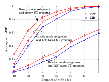
Figure 2: Average minimum MSP with mode assignment Algorithm 1 and UT grouping Algorithm 4, where $N=12$, and $K=20$.

1) Performance of the Proposed Greedy Mode Assignment and Greedy UT Grouping: Here, we investigate the performance of the proposed greedy mode assignment in Algorithm 1 and greedy UT grouping Algorithm 4 for PZF and MR combining schemes. We benchmark $1)$ random mode assignment, $2)$ UT grouping based on the value of large-scale fading coefficient $\beta_{mk}^{\mathtt{O}}$ (LSF-based UT grouping), so that when $N>K$ all UTs are assigned to $\mathcal{W}_{m}$ for ZF combining, $\forall m$, and when $N\leq K$ at MN $m$ a UT with the smallest value of $\beta_{mk}^{\mathtt{O}}$ is assigned into the $\mathcal{W}_{m}$ group for ZF combining and the remaining UTs are assigned into the $\mathcal{S}_{m}$ group for MR combining. Figure 2 illustrates the minimum MSP achieved by the CF-mMIMO surveillance system for different number of MNs $M$. In this initial evaluation, the setup consists in $D=1$ km, $N=12$, and $K=20$. Our results verify the advantage of the proposed greedy mode assignment over random mode assignment. More specifically, when $M=30$, greedy mode assignment provides performance gains of around $245\%$ and $325\%$ with respect to random mode assignment for the system relying on PZF combining and MR combining, respectively. This remarkable performance gain verifies the importance of an adequate mode selection in terms of monitoring performance in our CF-mMIMO surveillance system. Additionally, compared to the LSF-based grouping scheme, our proposed UT grouping provides up to an additional $100\%$ improvement in terms of MSP. This is reasonable because, PZF combining employing our proposed UT grouping can achieve an attractive balance between mitigating the interference and increasing the array gain. In the next figures, we present results for the scenarios associated with greedy mode assignment and greedy UT grouping.

2) Performance of the Proposed Max-Min MSP: Now, we examine the efficiency of proposed Max-Min MSP using power control and MN-weighting coefficient control provided by Algorithm 3 for the PZF and MR combining schemes. Our numerical results (not shown here) demonstrated that Algorithm 3 converges quickly, and hence in what follows we set the maximum number of iterations to $I=2$ for Algorithm 3. Figure 3 presents the minimum MSP of the CF-mMIMO surveillance system for different numbers of antennas per MN for systems having the same total numbers of service antennas, i.e., $N_{\mathtt{tot}}=NM=240$, but different number of MNs. We investigate three cases: case-$1$) equal power allocation and equal MN-weighting coefficient control, case-$2$) proposed power control but no optimal MN-weighting coefficient ($\alpha_{mk}=1$ and $\theta_{mk}$ is calculated from Algorithm 2), case-$3$) power control and optimal MN-weighting coefficient control Algorithm 3. The main observations that follow from these simulations are as follows:

• The max-min MSP power control and MN-weighting coefficient control enhance the system performance significantly for both the PZF and MR combining schemes. In particular, for the PZF combining scheme, compared to the case-$1$, i.e., equal power control and equal MN-weighting coefficient control, the power control provides a performance gain of up to $35\%$, while the power control together with the MN-weighting coefficient control can provide a performance gain of up to $43\%$. This highlights the advantage of our proposed solution, which becomes more pronounced for the PZF combining scheme.

  

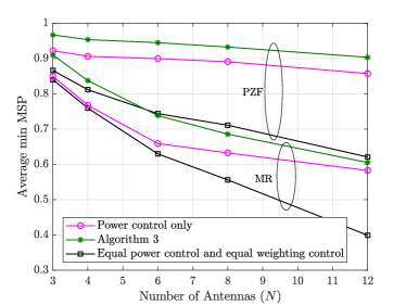
  Figure 3: Average minimum MSP with max-min MSP optimization (33), where $K=20$ and $N_{\mathtt{tot}}=240$.

• The monitoring performance gap between the MR combining and the PZF combining is quite significant. In particular, when $N=12$, applying PZF combining leads to $50\%$ improvement in terms of MSP with respect to the MR combining scheme. The reason is two-fold: Firstly, the ability of the PZF combining to cancel the cross-link interference; Secondly, the proposed power control and MN-weighting coefficient control along with the UT grouping scheme can notably enhance the monitoring performance of weak UTs. We also note that, the performance gap between PZF and MR combining schemes increases upon increasing $N$. The intuitive reason is that for a fixed total number of antennas, when the number of antennas per MN increases, the number of MN reduces. For a low number of MNs, the cross-link interference becomes dominant, which significantly degrades the overall performance of the system relying on MR combining.

• When $N$ increases, the performance of the MR and PZF combining schemes deteriorates. This is due to the fact that increasing $N$ and accordingly decreasing $M$ has two effects on the MSP, namely, (i) increases the diversity and array gains (a positive effect), and (ii) reduces the macro-diversity gain and increases the path loss due to an increase in the relative distance between the MNs and the untrusted pairs (a negative effect). The latter effect becomes dominant, which leads to a degradation in the monitoring performance.

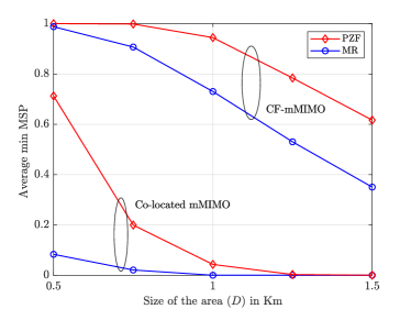
Figure 4: Average minimum MSP versus the size of the area, $D$, where $M=40$, $N=6$, and $K=20$.

3) CF-mMIMO versus Co-located Surveillance System: Now, we compare the MSP of the CF-mMIMO against that of a co-located FD massive MIMO system. The co-located FD massive MIMO surveillance system can be considered as a special case of the CF-mMIMO system, where all $M$ MNs are co-located as an antenna array, which simultaneously performs observation and jamming at the same frequency. Therefore, the effective SINR of the untrusted link and the effective SINR for observing at the CPU can be obtained by setting $\beta_{mk}^{\mathtt{O}}=\beta_{ik}^{\mathtt{O}}=\beta_{k}^{\mathtt{O}},\beta_{mk}^{\mathtt{J}}=\beta_{ik}^{\mathtt{J}}=\beta_{k}^{\mathtt{J}}$, $\gamma_{mk}^{\mathtt{O}}=\gamma_{ik}^{\mathtt{O}}=\gamma_{k}^{\mathtt{O}},\gamma_{mk}^{\mathtt{J}}=\gamma_{ik}^{\mathtt{J}}=\gamma_{k}^{\mathtt{J}}$, $\beta_{mi}=\sigma^{2}_{\mathtt{SI}},\forall m,i,k$ in Propositions 1, 2, and 3, respectively. Here, $\sigma^{2}_{\mathtt{SI}}$ reflects the strength of the residual self interference after employing self-interference suppression techniques [40]. Recall that in our CF-mMIMO surveillance system all MNs operate in half-duplex mode, hence there is no self interference at each MN.

For fair comparison with the CF-mMIMO system, the co-located system deploys the same total number of antennas, i.e., $N_{\mathtt{cl}}=\frac{N_{\mathtt{tot}}}{2}=\frac{NM}{2}$ antennas are used for observing, while ${N_{\mathtt{cl}}}$ antennas are used for jamming, which is termed as “an antenna-preservation” condition [41]. Accordingly, the effective SINR of the untrusted link $k$ for FD co-located massive MIMO systems can be written as

$$\mathtt{SINR}_{\mathtt{UR},k}^{\mathtt{cl}}(\bm{\theta})=\frac{\rho_{\mathtt{UT}}|h_{kk}|^{2}}{\xi_{k}(\bm{\theta})},$$ (44)

where

$$\xi_{k}(\bm{\theta})= \rho_{\mathtt{UT}}\!\!\!\sum_{\ell\in\mathcal{K}\setminus k}\!\!\beta_{\ell k}^{\mathtt{U}}\!+{\rho_{\mathtt{J}}}N_{\mathtt{cl}}\sum_{k^{\prime}\in\mathcal{K}}\!\!\theta_{k^{\prime}}\beta_{k}^{\mathtt{J}}\gamma_{k^{\prime}}^{\mathtt{J}}\!\!+\!{\rho_{\mathtt{J}}}N_{\mathtt{cl}}^{2}\!{\theta_{k}}(\gamma_{k}^{\mathtt{J}})^{2}\!+\!1.$$

Additionally, the received SINR of the $k$-th untrusted link at the CPU for MR combining in our FD co-located massive MIMO system is given by

$$\mathtt{SINR}_{\mathtt{O},k}^{\mathtt{cl},\mathtt{MR}}(\bm{\theta})=\frac{N_{\mathtt{cl}}\rho_{\mathtt{UT}}(\gamma_{k}^{\mathtt{O}})^{2}}{\mu_{k}^{\mathtt{cl},\mathtt{MR}}+\rho_{\mathtt{J}}N_{\mathtt{cl}}\sum\nolimits_{\ell\in\mathcal{K}}\!\theta_{\ell}\gamma_{\ell}^{\mathtt{J}}\varrho_{k}^{\mathtt{cl},\mathtt{MR}}},$$ (45)

with $\mu_{k}^{\mathtt{cl},\mathtt{MR}}=\rho_{\mathtt{UT}}\sum\nolimits\nolimits_{\ell\in\mathcal{K}}\beta_{\ell}^{\mathtt{O}}\gamma_{k}^{\mathtt{O}}+\gamma_{k}^{\mathtt{O}}$, and $\varrho_{k}^{\mathtt{cl},\mathtt{MR}}=\gamma_{k}^{\mathtt{O}}\sigma^{2}_{\mathtt{SI}}$, while the received SINR for the $k$-th untrusted link for full ZF combining and $N_{\mathtt{cl}}\geq K+1$ is given by

$$\mathtt{SINR}_{\mathtt{O},k}^{\mathtt{cl},\mathtt{ZF}}(\bm{\theta})=\frac{\rho_{\mathtt{UT}}({\gamma_{k}^{\mathtt{O}}})^{2}}{\mu_{k}^{\mathtt{cl},\mathtt{ZF}}+\rho_{\mathtt{J}}N_{\mathtt{cl}}\sum\nolimits_{\ell\in\mathcal{K}}\theta_{\ell}{\gamma_{\ell}^{\mathtt{J}}}\varrho_{k}^{\mathtt{cl},\mathtt{ZF}}},$$ (46)

with $\mu_{k}^{\mathtt{cl},\mathtt{ZF}}=\rho_{\mathtt{UT}}\sum\nolimits_{\ell\in\mathcal{K}}\!\frac{\gamma_{k}^{\mathtt{O}}(\beta_{\ell}^{\mathtt{O}}-\gamma_{\ell}^{\mathtt{O}})}{N_{\mathtt{cl}}-K}+\frac{\gamma_{k}^{\mathtt{O}}}{N_{\mathtt{cl}}-K}$ and $\varrho_{k}^{\mathtt{cl},\mathtt{ZF}}=\frac{\gamma_{k}^{\mathtt{O}}\sigma^{2}_{\mathtt{SI}}}{N_{\mathtt{cl}}-K}$.

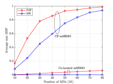
Figure 5: Average minimum MSP versus number of MNs, $M$, where $N=4$, and $K=20$.

For co-located massive MIMO systems, unless otherwise stated, we assume that the residual self interference after employing a self-interference suppression technique is $\sigma^{2}_{\mathtt{SI}}/\sigma_{n}^{2}=30$ dB. In addition, we adopt a similar power control principle as in Algorithm 2. Figure 4 shows the minimum MSP versus the size of the area, $D$. It can be observed that the CF-mMIMO surveillance system significantly outperforms its co-located massive MIMO counterpart. As expected, the relative performance gap between CF-mMIMO and co-located surveillance systems dramatically escalates with the size of the area $D$. For example, for $D=0.75$ km, the CF-mMIMO system provides around $5$-fold improvement in the minimum MSP performance over the co-located system, while the improvement reaches a $40$-fold value for $D=1$ km. This highlights the effectiveness of our optimized CF-mMIMO surveillance scheme for proactive monitoring systems. The reason is the capability of the CF-mMIMO to surround each UT and each UR by relying on MNs operating in observing and jamming mode, respectively. Additionally, in contrast to our CF-mMIMO with distributed MNs, a co-located massive MIMO suffers from excessive self-interference due to the short distance between the transmit and receive antennas of a single large MN.

4) Effect of the Number of MNs: Figure 5 shows the minimum MSP versus the number of MNs, $M$. For our CF-mMIMO system using the MR and PZF combining schemes, when the number of MNs increases, the macro-diversity gain increases, and hence the MSP enhances. Upon increasing $M$, for co-located massive MIMO the number of transmit and receive antennas increases, which results in a higher array gain and monitoring performance. In particular, we can see that the surveillance systems can benefit much more from the higher macro-diversity gain in a CF-mMIMO network, rather than from the higher array gain attained in co-located networks.

The results shown both in Fig. 4 as well as in Fig. 5 clearly suggest that having a high degree of macro diversity and low path loss are crucial for offering a high MSP and corroborate that CF-mMIMO is well-suited for the surveillance of networks in wide areas.

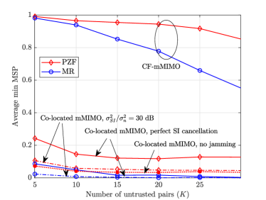
Figure 6: Average minimum MSP versus number of untrusted links, $K$, where $M=40$ and $N=6$.

5) Effect of the Number of Untrusted Links: Next, in Fig. 6, we investigate the impact of the number of untrusted links on the MSP performance of both CF-mMIMO and of co-located massive MIMO systems. Herein, we also consider co-located massive MIMO having perfect SI cancellation and half-duplex co-located massive MIMO with no jamming. We observe that upon increasing $K$, the monitoring performance of all schemes deteriorates. Nevertheless, the CF-mMIMO system using the PZF combining scheme still yields excellent MSP compared to the other schemes. We also note that for small values of $K$, MR combining provides a better performance/implementation complexity trade-off compared to its PZF counterpart. However, increasing the number of untrusted pairs results in stronger cross-link interference. Therefore, PZF combining having the ability to cancel the cross-link interference is undoubtedly a better choice. Interestingly, we can observe that even under the idealized assumption of having perfect SI cancellation in co-located massive MIMO, CF-mMIMO surveillance still significantly outperforms the co-located massive MIMO. This result shows that the proposed CF-mMIMO surveillance system, relying on the proposed power control, MN-weighting coefficient control, and suitable mode assignment, yields an impressive monitoring performance in multiple untrusted pair scenarios.

VI Conclusions

We have developed a CF-mMIMO surveillance system for monitoring multiple distributed untrusted pairs and analyzed the performance of both MR and PZF combining schemes. We proposed a new long-term-based optimization technique of designing the MN mode assignment, power control for the MNs that are in jamming mode, and MN-weighting coefficients to maximize the min MSP across all untrusted pairs under practical transmit power constraints. We showed that our CF-mMIMO surveillance systems provide significant monitoring gains over conventional co-located massive MIMO, even for relatively small number of MNs. In particular, the minimum MSP of CF-mMIMO surveillance is an order of magnitude higher than that of the co-located massive MIMO system, when the untrusted pairs are spread out over a large area. The results also show that with different network setups, PZF combining provides the highest MSP, while for small values of the number of untrusted pairs and the size of the area, MR combining constitutes a beneficial choice.

Appendix A Proof of Proposition 1

To derive a closed-form expression for the effective SINR of the untrusted link, we have to calculate $\xi_{k}({\bf a},\bm{\theta})=\mathbb{E}\Big{\{}\big{|}\tilde{w}_{k}^{\mathtt{UR}}\big{|}^{2}\Big{\}}$. Let us denote the jamming channel estimation error by $\bm{\varepsilon}_{mk}^{\mathrm{J}}={\bf g}_{mk}^{\mathtt{J}}-\hat{{\bf g}}_{mk}^{\mathtt{J}}$. Therefore, we have

$$\xi_{k}({\bf a},\bm{\theta})=\mathbb{E}\Big{\{}\big{|}\tilde{w}_{k}^{\mathtt{UR}}\big{|}^{2}\Big{\}}=\rho_{\mathtt{UT}}\sum_{\ell\in\mathcal{K}\setminus k}\beta_{\ell k}^{\mathtt{U}}+{\rho_{\mathtt{J}}}\mathcal{I}+1,$$ (47)

where

$$\mathcal{I}\triangleq \sum_{k^{\prime}\in\mathcal{K}}\mathbb{E}\Big{\{}\Big{|}\sum_{m\in\mathcal{M}}a_{m}\sqrt{\theta_{mk^{\prime}}}({\bf g}_{mk}^{\mathtt{J}})^{T}\left(\hat{{\bf g}}_{mk^{\prime}}^{\mathtt{J}}\right)^{*}\Big{|}^{2}\Big{\}}.$$

To calculate $\mathcal{I}$, owing to the fact that the variance of a sum of independent RVs is equal to the sum of the variances, we have

$$\mathcal{I}\stackrel{{\scriptstyle(a)}}{{=}}\!\sum_{k^{\prime}\in\mathcal{K}\setminus k}\!\!\mathbb{E}\Big{\{}\big{|}\!\sum_{m\in\mathcal{M}}\!\!a_{m}\sqrt{\theta_{mk^{\prime}}}\left({\bf g}_{mk}^{\mathtt{J}}\right)^{T}\left(\hat{{\bf g}}_{mk^{\prime}}^{\mathtt{J}}\right)^{*}\big{|}^{2}\Big{\}}$$

$$\qquad+\!\mathbb{E}\Big{\{}\Big{|}\sum_{m\in\mathcal{M}}\!\!a_{m}\sqrt{\theta_{mk}}\left(\bm{\varepsilon}_{mk}^{\mathrm{J}}\!+\!\hat{{\bf g}}_{mk}^{\mathtt{J}}\right)^{T}\left(\hat{{\bf g}}_{mk}^{\mathtt{J}}\right)^{*}\Big{|}^{2}\Big{\}}$$

$$\!\!\stackrel{{\scriptstyle(b)}}{{=}}\!\!\!\sum_{k^{\prime}\in\mathcal{K}\setminus k}\sum_{m\in\mathcal{M}}\!\!\!a_{m}{\theta_{mk^{\prime}}}\mathbb{E}\!\Big{\{}\!\left({\bf g}_{mk}^{\mathtt{J}}\right)^{T}\!\!\mathbb{E}\Big{\{}\!\left(\hat{{\bf g}}_{mk^{\prime}}^{\mathtt{J}}\right)^{*}\!\!\left(\hat{{\bf g}}_{mk^{\prime}}^{\mathtt{J}}\right)^{T}\!\!\Big{\}}\left({\bf g}_{mk}^{\mathtt{J}}\right)^{*}\!\!\Big{\}}$$

$$\hskip 20.00003pt+\sum_{m\in\mathcal{M}}a_{m}\theta_{mk}\left(\mathbb{E}\Big{\{}\big{\|}\hat{{\bf g}}_{mk}^{\mathtt{J}}\big{\|}^{4}\Big{\}}+\mathbb{E}\Big{\{}\big{|}{(\bm{\varepsilon}}_{mk}^{\mathrm{J}})^{T}(\hat{{\bf g}}_{mk}^{\mathtt{J}})^{*}\big{|}^{2}\!\Big{\}}\!\right)$$

$$\hskip 20.00003pt+\sum_{m\in\mathcal{M}}\sum_{n\in\mathcal{M}\setminus m}a_{m}a_{n}\sqrt{\theta_{mk}\theta_{nk}}\mathbb{E}\Big{\{}\|\hat{{\bf g}}_{mk}^{\mathtt{J}}\|^{2}\!\Big{\}}\mathbb{E}\Big{\{}\|\hat{{\bf g}}_{nk}^{\mathtt{J}}\|^{2}\!\Big{\}}$$

$$\stackrel{{\scriptstyle(c)}}{{=}}N\!\!\sum_{k^{\prime}\in\mathcal{K}\setminus k}\sum_{m\in\mathcal{M}}a_{m}\theta_{mk^{\prime}}\beta_{mk}^{\mathtt{J}}\gamma_{mk^{\prime}}^{\mathtt{J}}+\!N\!\!\sum_{m\in\mathcal{M}}\!\!a_{m}\theta_{mk}\gamma_{mk}^{\mathtt{J}}(N\times$$

$$\qquad\gamma_{mk}^{\mathtt{J}}+\beta_{mk}^{\mathtt{J}})+N^{2}\sum_{m\in\mathcal{M}}\sum_{n\in\mathcal{M}\setminus m}a_{m}a_{n}\sqrt{\theta_{mk}\theta_{nk}}\gamma_{mk}^{\mathtt{J}}\gamma_{nk}^{\mathtt{J}}$$

$$=\!N\!\!\sum_{k^{\prime}\in\mathcal{K}}\sum_{m\in\mathcal{M}}a_{m}\theta_{mk^{\prime}}\beta_{mk}^{\mathtt{J}}\gamma_{mk^{\prime}}^{\mathtt{J}}+N^{2}\Big{(}\!\sum_{m\in\mathcal{M}}\!\!a_{m}\sqrt{\theta_{mk}}\gamma_{mk}^{\mathtt{J}}\!\Big{)}^{2}\!\!,$$ (48)

where $(a)$ follows from the fact that $\hat{{\bf g}}_{mk^{\prime}}^{\mathtt{J}}$ has zero mean and it is independent of ${\bf g}_{mk}^{\mathtt{J}}$ and $\hat{{\bf g}}_{mk}^{\mathtt{J}}$, $(b)$ follows from the fact that $\bm{\varepsilon}_{mk}^{\mathrm{J}}$ is independent of $\hat{{\bf g}}_{mk^{\prime}}^{\mathtt{J}}$ and it is a zero-mean RV and $(c)$ follows from the fact that $\mathbb{E}\big{\{}\|\hat{{\bf g}}_{mk}^{\mathtt{J}}\|^{4}\big{\}}=N(N+1)(\gamma_{mk}^{\mathtt{J}})^{2}$. Substituting (A) into (47) completes the proof.

Appendix B Proof of Proposition 2

Let us denote the observing channel estimation error, which is independent of $\hat{\bf g}_{mk}^{\mathtt{O}}$ and zero-mean RV, by $\bm{\varepsilon}_{mk}^{\mathtt{O}}={\bf g}_{mk}^{\mathtt{O}}-\hat{\bf g}_{mk}^{\mathtt{O}}$. According to ${{\bf v}}_{mk}^{\mathtt{MR}}=\hat{{\bf g}}_{mk}^{\mathtt{O}}$ and by exploiting the independence between the channel estimation errors and the estimates, we have

$$\mathbb{E}\big{\{}\text{DS}_{k}^{\mathtt{MR}}\} \!=\!\sqrt{{\rho_{\mathtt{UT}}}}\sum\limits_{m\in{\mathcal{M}}}\!\!\alpha_{mk}(1\!-\!a_{m})\mathbb{E}\left\{{(\hat{{\bf g}}_{mk}^{\mathtt{O}})^{\dagger}}(\hat{{\bf g}}_{mk}^{\mathtt{O}}\!+\!{\bm{\varepsilon}}_{mk}^{\mathtt{O}})\right\}$$

$$=\sqrt{{\rho_{\mathtt{UT}}}}\sum\limits_{m\in{\mathcal{M}}}\alpha_{mk}(1-a_{m})N\gamma_{mk}^{\mathtt{O}}.$$ (49)

Additionally, $\mathbb{E}\big{\{}|\text{BU}_{k}^{\mathtt{MR}}|^{2}\big{\}}$ can be written as

$$\mathbb{E}\big{\{}|\text{BU}_{k}^{\mathtt{MR}}|^{2}\big{\}}$$

$$=\!{\rho_{\mathtt{UT}}}\sum\limits_{m\in{\mathcal{M}}}\alpha_{mk}^{2}(1\!-\!a_{m})\mathbb{E}\Big{\{}|{(\hat{{\bf g}}_{mk}^{\mathtt{O}})^{\dagger}}{\bf g}_{mk}^{\mathtt{O}}\!-\!\mathbb{E}\{{(\hat{{\bf g}}_{mk}^{\mathtt{O}})^{\dagger}}{\bf g}_{mk}^{\mathtt{O}}\}{|^{2}}\!\Big{\}}$$

$$=\!\rho_{\mathtt{UT}}\!\!\!\sum\limits_{m\in{\mathcal{M}}}\alpha_{mk}^{2}(1-a_{m})\Big{(}\!{\mathbb{E}}\Big{\{}\big{|}{(\hat{{\bf g}}_{mk}^{\mathtt{O}})^{\dagger}}\bm{\varepsilon}_{mk}^{\mathtt{O}}\!+\!\|\hat{{\bf g}}_{mk}^{\mathtt{O}}{\|^{2}}{\big{|}^{2}}\!\Big{\}}$$

$$\hskip 100.00015pt\!-\!N^{2}(\gamma_{mk}^{\mathtt{O}})^{2}\!\Big{)}$$

$$\stackrel{{\scriptstyle(a)}}{{=}}\rho_{\mathtt{UT}}\sum\limits_{m\in{\mathcal{M}}}\alpha_{mk}^{2}(1-a_{m})\big{(}\mathbb{E}\big{\{}|{(\hat{{\bf g}}_{mk}^{\mathtt{O}})^{\dagger}}\bm{\varepsilon}_{mk}^{\mathtt{O}}{|^{2}}\big{\}}$$

$$\hskip 100.00015pt+\mathbb{E}\big{\{}\|\hat{{\bf g}}_{mk}^{\mathtt{O}}{\|^{4}}\big{\}}-N^{2}(\gamma_{mk}^{\mathtt{O}})^{2}\big{)}$$

$$\stackrel{{\scriptstyle(b)}}{{=}}\rho_{\mathtt{UT}}\sum\limits_{m\in{\mathcal{M}}}\alpha_{mk}^{2}(1-a_{m})N\beta_{mk}^{\mathtt{O}}\gamma_{mk}^{\mathtt{O}},$$ (50)

where we have exploited that: in $(a)$ $\bm{\varepsilon}_{mk}^{\mathtt{O}}$ is independent of $\hat{\bf g}_{mk}^{\mathtt{O}}$ and a zero-mean RV; in $(b)$ $\mathbb{E}\big{\{}\|\hat{{\bf g}}_{mk}^{\mathtt{O}}\|^{4}\big{\}}=N(N+1)(\gamma_{mk}^{\mathtt{O}})^{2}$.

By exploiting the fact that $\hat{{\bf g}}_{mk}^{\mathtt{O}}$ is independent of ${{\bf g}}_{m\ell}^{\mathtt{O}}$ for $k\neq\ell$, while $\hat{{\bf g}}_{mk}^{\mathtt{O}}$, ${{\bf F}_{mi}}$, and ${\mathbf{\hat{g}}}_{i\ell}^{\mathtt{J}}$ are independent, we can formulate $\mathbb{E}\{|{\text{UI}}_{\ell k}^{\mathtt{MR}}|^{2}\}$ and $\mathbb{E}\{|\text{MI}_{\ell k}^{\mathtt{MR}}|^{2}\}$, respectively, as

$$\mathbb{E}\big{\{}|{\text{UI}}_{\ell k}^{\mathtt{MR}}|^{2}\big{\}}={\rho_{\mathtt{UT}}}{\sum\limits_{m\in{\mathcal{M}}}}\alpha_{mk}^{2}(1-a_{m})N\gamma_{mk}^{\mathtt{O}}\beta_{m\ell}^{\mathtt{O}},$$ (51)

$$\mathbb{E}\big{\{}|\text{MI}_{\ell k}^{\mathtt{MR}}|^{2}\big{\}}$$

$$={\rho_{\mathtt{J}}}\sum\limits_{m\in{\mathcal{M}}}\sum\limits_{i\in{\mathcal{M}}}\alpha_{mk}^{2}(1-a_{m})a_{i}\theta_{i\ell}\mathbb{E}\{|{({\mathbf{\hat{g}}}_{mk}^{\mathtt{O}})^{H}}{{\mathbf{F}}_{mi}}{({\mathbf{\hat{g}}}_{i\ell}^{\mathtt{J}})^{\ast}}{|^{2}}\}$$

$$={\rho_{\mathtt{J}}}{\sum\limits_{m\in{\mathcal{M}}}{\sum\limits_{i\in{\mathcal{M}}}}}\alpha_{mk}^{2}N^{2}(1-a_{m})a_{i}\theta_{i\ell}\gamma_{mk}^{\mathtt{O}}\beta_{mi}\gamma_{i\ell}^{\mathtt{J}}.$$ (52)

The substitution of (B), (B), (51), and (52) into (III-B) and inserting $\mathbb{E}\big{\{}|\text{AN}_{k}^{\mathtt{MR}}|^{2}\big{\}}=\!N\sum\nolimits_{m\in{\mathcal{M}}}\alpha_{mk}^{2}(1-a_{m})\gamma_{mk}^{\mathtt{O}}$, yields (20).

Appendix C Proof of Proposition 3

According to (11) and due to the fact that ${\bm{\varepsilon}}_{mk}^{\mathtt{O}}$ has zero mean and is independent of $\hat{{\bf g}}_{mk}^{\mathtt{O}}$, $\mathbb{E}\{\text{DS}_{k}^{\mathtt{PZF}}\}$ in the numerator of (III-B) can be calculated as

$$\mathbb{E}\{\text{DS}_{k}^{\mathtt{PZF}}\}\!=\!\!\sqrt{{\rho_{\mathtt{UT}}}}\Big{(}\!\!\sum\limits_{m\in\mathcal{Z}_{k}}\!\!\alpha_{mk}(1\!\!-\!a_{m})\mathbb{E}\left\{{({{\bf v}}_{mk}^{\mathtt{ZF}})^{\dagger}}(\hat{{\bf g}}_{mk}^{\mathtt{O}}\!+\!{\bm{\varepsilon}}_{mk}^{\mathtt{O}})\right\}$$

$$\hskip 30.00005pt+\sum\limits_{m\in\mathcal{M}_{k}}\alpha_{mk}(1-a_{m})\mathbb{E}\left\{{({{\bf v}}_{mk}^{\mathtt{MR}})^{\dagger}}(\hat{{\bf g}}_{mk}^{\mathtt{O}}+{\bm{\varepsilon}}_{mk}^{\mathtt{O}})\right\}\Big{)}$$

$$=\sqrt{{\rho_{\mathtt{UT}}}}\Big{(}\sum\limits_{m\in\mathcal{Z}_{k}}\alpha_{mk}(1-a_{m})\gamma_{mk}^{\mathtt{O}}$$

$$\hskip 30.00005pt+N\sum\limits_{m\in\mathcal{M}_{k}}\alpha_{mk}(1-a_{m})\gamma_{mk}^{\mathtt{O}}\Big{)}.$$ (53)

Then, $\mathbb{E}\big{\{}|{\text{BU}}_{k}^{\mathtt{PZF}}|^{2}\big{\}}$ can be written as

$$\mathbb{E}\big{\{}|\text{BU}_{k}^{\mathtt{PZF}}|^{2}\big{\}}={\rho_{\mathtt{UT}}}\mathbb{E}\Big{\{}\big{|}\sum\limits_{m\in\mathcal{Z}_{k}}\alpha_{mk}(1\!-\!a_{m}){({{\bf v}}_{mk}^{\mathtt{ZF}})^{\dagger}}{\bf g}_{mk}^{\mathtt{O}}+$$

$$\sum\limits_{m\in\mathcal{M}_{k}}\alpha_{mk}(1\!-\!a_{m}){({{\bf v}}_{mk}^{\mathtt{MR}})^{\dagger}}{\bf g}_{mk}^{\mathtt{O}}\big{|}^{2}\Big{\}}-{\rho_{\mathtt{UT}}}\big{|}\mathbb{E}\big{\{}\sum\limits_{m\in\mathcal{Z}_{k}}\alpha_{mk}$$

$$(1\!-\!a_{m}){({{\bf v}}_{mk}^{\mathtt{ZF}})^{\dagger}}{\bf g}_{mk}^{\mathtt{O}}+\sum\limits_{m\in\mathcal{M}_{k}}\alpha_{mk}(1\!-\!a_{m}){({{\bf v}}_{mk}^{\mathtt{ZF}})^{\dagger}}{\bf g}_{mk}^{\mathtt{O}}\big{\}}\big{|}^{2}$$

$$=\rho_{\mathtt{UT}}\mathcal{I}_{2}-|\mathbb{E}\big{\{}\text{DS}_{k}^{\mathtt{PZF}}\}|^{2},$$ (54)

where

$$\mathcal{I}_{2}= \mathbb{E}\Big{\{}\big{|}\sum\nolimits_{m\in\mathcal{Z}_{k}}\alpha_{mk}(1\!-\!a_{m}){({{\bf v}}_{mk}^{\mathtt{ZF}})^{\dagger}}{\bf g}_{mk}^{\mathtt{O}}+$$

$$\sum\nolimits_{m\in\mathcal{M}_{k}}\alpha_{mk}(1\!-\!a_{m}){({{\bf v}}_{mk}^{\mathtt{MR}})^{\dagger}}{\bf g}_{mk}^{\mathtt{O}}\big{|}^{2}\Big{\}}.$$ (55)

By applying

$$\mathbb{E}\Big{\{}\big{\|}{{\bf v}}_{mk}^{\mathtt{ZF}}\big{\|}^{2}\Big{\}} =(\gamma_{mk}^{\mathtt{O}})^{2}\mathbb{E}\Big{\{}\big{\|}\hat{{\bf G}}_{\mathcal{W}_{m}}^{\mathtt{O}}\big{(}(\hat{{\bf G}}_{\mathcal{W}_{m}}^{\mathtt{O}})^{\dagger}\hat{{\bf G}}_{\mathcal{W}_{m}}^{\mathtt{O}}\big{)}^{-1}{\bf e}_{k}\big{\|}^{2}\Big{\}}$$

$$=\frac{\gamma_{mk}^{\mathtt{O}}}{N-|\mathcal{W}_{m}|},$$ (56)

which follows from [42, Lemma 2.10], we have

$$\mathcal{I}_{2}\stackrel{{\scriptstyle(a)}}{{=}}\big{(}\sum_{m\in\mathcal{Z}_{k}}\alpha_{mk}(1-a_{m})\gamma_{mk}^{\mathtt{O}}\big{)}^{2}\!+\!\sum_{m\in\mathcal{Z}_{k}}\alpha_{mk}^{2}(1-a_{m})\times$$

$$\frac{\gamma_{mk}^{\mathtt{O}}(\beta_{mk}^{\mathtt{O}}\!\!-\!\gamma_{mk}^{\mathtt{O}})}{N-|\mathcal{W}_{m}|}+\mathbb{E}\Big{\{}\big{|}\!\!\sum\limits_{m\in\mathcal{M}_{k}}\alpha_{mk}(1\!-\!a_{m})({{\bf v}}_{mk}^{\mathtt{MR}})^{\dagger}{\bf g}_{mk}^{\mathtt{O}}\big{\}}\big{|}^{2}\Big{\}}$$

$$+2\big{(}\!\sum_{m\in\mathcal{Z}_{k}}\alpha_{mk}(1-a_{m})\gamma_{mk}^{\mathtt{O}}\Big{)}\Big{(}N\sum_{m\in\mathcal{M}_{k}}\!\!\alpha_{mk}(1-a_{m})\gamma_{mk}^{\mathtt{O}}\big{)}.$$ (57)

Also, the third term of $\mathcal{I}_{2}$ can be calculated as

$$\mathbb{E}\Big{\{}\big{|}\sum\nolimits_{m\in\mathcal{M}_{k}}\alpha_{mk}(1\!-\!a_{m})({{\bf v}}_{mk}^{\mathtt{MR}})^{\dagger}{\bf g}_{mk}^{\mathtt{O}}\big{\}}\big{|}^{2}\Big{\}}$$

$$~{}~{}=\sum\nolimits_{m\in\mathcal{M}_{k}}\alpha_{mk}^{2}(1\!-\!a_{m})\mathbb{E}\big{\{}|({{\bf v}}_{mk}^{\mathtt{MR}})^{\dagger}{\bf g}_{mk}^{\mathtt{O}}|^{2}\big{\}}$$

$$\qquad+\Big{|}\sum\nolimits_{m\in\mathcal{M}_{k}}\alpha_{mk}(1\!-\!a_{m})\mathbb{E}\big{\{}({{\bf v}}_{mk}^{\mathtt{MR}})^{\dagger}{\bf g}_{mk}^{\mathtt{O}}\big{\}}\Big{|}^{2}$$

$$\qquad-\sum\nolimits_{m\in\mathcal{M}_{k}}(1\!-\!a_{m})\big{|}\alpha_{mk}\mathbb{E}\big{\{}({{\bf v}}_{mk}^{\mathtt{MR}})^{\dagger}{\bf g}_{mk}^{\mathtt{O}}\big{\}}\big{|}^{2}$$

$$~{}~{}=\sum\nolimits_{m\in\mathcal{M}_{k}}\alpha_{mk}^{2}(1\!-\!a_{m})N\beta_{mk}^{\mathtt{O}}\gamma_{mk}^{\mathtt{O}}$$

$$\qquad+\Big{(}\sum\nolimits_{m\in\mathcal{M}_{k}}\alpha_{mk}(1\!-\!a_{m})N\gamma_{mk}^{\mathtt{O}}\Big{)}^{2}.$$ (58)

Substituting (C) into (C) and then (C) and (C) into (C) yields

$$\mathbb{E}\big{\{}|\text{BU}_{k}^{\mathtt{PZF}}|^{2}\}= \rho_{\mathtt{UT}}\sum_{m\in\mathcal{Z}_{k}}\alpha_{mk}^{2}(1-a_{m})\frac{\gamma_{mk}^{\mathtt{O}}(\beta_{mk}^{\mathtt{O}}-\gamma_{mk}^{\mathtt{O}})}{N-|\mathcal{W}_{m}|}+$$

$$\rho_{\mathtt{UT}}\sum\limits_{m\in\mathcal{M}_{k}}\alpha_{mk}^{2}(1\!-\!a_{m})N\beta_{mk}^{\mathtt{O}}\gamma_{mk}^{\mathtt{O}}.$$ (59)

Similarly, we compute $\text{UI}_{\ell k}^{\mathtt{PZF}}$ as

$$\mathbb{E}\big{\{}|\text{UI}_{\ell k}^{\mathtt{PZF}}|^{2}\} =\rho_{\mathtt{UT}}\sum_{m\in\mathcal{Z}_{k}}\alpha_{mk}^{2}(1-a_{m})\frac{\gamma_{mk}^{\mathtt{O}}(\beta_{m\ell}^{\mathtt{O}}-\gamma_{m\ell}^{\mathtt{O}})}{N-|\mathcal{W}_{m}|}$$

$$+\rho_{\mathtt{UT}}\sum\limits_{m\in\mathcal{M}_{k}}\alpha_{mk}^{2}(1\!-\!a_{m})N\beta_{m\ell}^{\mathtt{O}}\gamma_{mk}^{\mathtt{O}}.$$ (60)

It can be shown that ${({{\bf v}}_{mk}^{\mathtt{ZF}})^{\dagger}}{{\bf F}_{mi}}{({\mathbf{\hat{g}}}_{i\ell}^{\mathtt{J}})^{\ast}}$ is a zero-mean RV with variance $\frac{N\gamma_{mk}^{\mathtt{O}}\beta_{mi}\gamma_{i\ell}^{\mathtt{J}}}{N-|\mathcal{W}_{m}|}$. Moreover, ${({{\bf v}}_{mk}^{\mathtt{MR}})^{\dagger}}{{\bf F}_{mi}}{({\mathbf{\hat{g}}}_{i\ell}^{\mathtt{J}})^{\ast}}$ is a zero-mean RV with variance ${N^{2}\gamma_{mk}^{\mathtt{O}}\beta_{mi}\gamma_{i\ell}^{\mathtt{J}}}$. Therefore, we can formulate $\mathbb{E}\big{\{}|\text{MI}_{\ell k}^{\mathtt{PZF}}|^{2}\}$ as

$$\mathbb{E}\big{\{}|\text{MI}_{\ell k}^{\mathtt{PZF}}|^{2}\}$$

$$={\rho_{\mathtt{J}}}\sum\limits_{i\in{\mathcal{M}}}a_{i}\theta_{i\ell}\Big{(}\sum\limits_{m\in\mathcal{Z}_{k}}\alpha_{mk}^{2}(1-a_{m})\mathbb{E}\{|{({{\bf v}}_{mk}^{\mathtt{ZF}})^{\dagger}}{{\mathbf{F}}_{mi}}{({\mathbf{\hat{g}}}_{i\ell}^{\mathtt{J}})^{\ast}}{|^{2}}\}$$

$$\qquad+\sum\limits_{m\in\mathcal{M}_{k}}\alpha_{mk}^{2}(1-a_{m})\mathbb{E}\{|{({{\bf v}}_{mk}^{\mathtt{MR}})^{\dagger}}{{\mathbf{F}}_{mi}}{({\mathbf{\hat{g}}}_{i\ell}^{\mathtt{J}})^{\ast}}{|^{2}}\}\Big{)}$$

$$={\rho_{\mathtt{J}}}N{\sum\limits_{i\in{\mathcal{M}}}}a_{i}{\theta_{i\ell}}\gamma_{i\ell}^{\mathtt{J}}\big{(}\sum\limits_{\begin{subarray}{c}m\in\mathcal{Z}_{k}\end{subarray}}\alpha_{mk}^{2}(1-a_{m})\frac{\gamma_{mk}^{\mathtt{O}}\beta_{mi}}{N-|\mathcal{W}_{m}|}$$

$$\qquad+N\!\sum\limits_{\begin{subarray}{c}m\in\mathcal{M}_{k}\end{subarray}}\alpha_{mk}^{2}(1-a_{m}){\gamma_{mk}^{\mathtt{O}}\beta_{mi}}\big{)}.$$ (61)

Finally, by exploiting the fact that the noise and the channel estimate are independent, $\mathbb{E}\big{\{}|\text{AN}_{k}^{\mathtt{PZF}}|^{2}\}$ can be written as

$$\mathbb{E}\big{\{}|\text{AN}_{k}^{\mathtt{PZF}}|^{2}\}=\mathbb{E}\Bigg{\{}\Big{|}\sum\limits_{m\in\mathcal{Z}_{k}}\alpha_{mk}(1\!-\!a_{m}){({{\bf v}}_{mk}^{\mathtt{ZF}})^{\dagger}}{\bf w}_{m}^{\mathtt{O}}\Big{|}^{2}\Bigg{\}}$$

$$\qquad+\mathbb{E}\Bigg{\{}\Big{|}\sum\limits_{m\in\mathcal{M}_{k}}\alpha_{mk}(1\!-\!a_{m}){({{\bf v}}_{mk}^{\mathtt{ZF}})^{\dagger}}{\bf w}_{m}^{\mathtt{O}}\Big{|}^{2}\Bigg{\}}$$

$$=\sum\limits_{\begin{subarray}{c}m\in\mathcal{Z}_{k}\end{subarray}}\!\alpha_{mk}^{2}(1\!\!-\!a_{m})\frac{\gamma_{mk}^{\mathtt{O}}}{N-|\mathcal{W}_{m}|}+N\!\sum\limits_{\begin{subarray}{c}m\in\mathcal{M}_{k}\end{subarray}}\!\!\alpha_{mk}^{2}(1\!\!-\!a_{m})\gamma_{mk}^{\mathtt{O}}.$$ (62)

The substitution of (C), (C), (C), (C), and (C) into (III-B) yields (3).

Zahra Mobini received the B.S. degree in electrical engineering from Isfahan University of Technology, Isfahan, Iran, in 2006, and the M.S and Ph.D. degrees, both in electrical engineering, from the M. A. University of Technology and K. N. Toosi University of Technology, Tehran, Iran, respectively. From November 2010 to November 2011, she was a Visiting Researcher at the Research School of Engineering, Australian National University, Canberra, ACT, Australia. She is currently a Post-Doctoral Research Fellow at the Centre for Wireless Innovation (CWI), Queen’s University Belfast (QUB). Before joining QUB, she was an Assistant and then Associate Professor with the Faculty of Engineering, Shahrekord University, Shahrekord, Iran (2015-2021). Her research interests include physical-layer security, massive MIMO, cell-free massive MIMO, full-duplex communications, and resource management and optimization. She has co-authored many research papers in wireless communications. She has actively served as the reviewer for a variety of IEEE journals, such as TWC, TCOM, and TVT.

Hien Quoc Ngo is currently a Reader with Queen’s University Belfast, U.K. His main research interests include massive MIMO systems, cell-free massive MIMO, reconfigurable intelligent surfaces, physical layer security, and cooperative communications. He has co-authored many research papers in wireless communications and co-authored the Cambridge University Press textbook Fundamentals of Massive MIMO (2016). He received the IEEE ComSoc Stephen O. Rice Prize in 2015, the IEEE ComSoc Leonard G. Abraham Prize in 2017, the Best Ph.D. Award from EURASIP in 2018, and the IEEE CTTC Early Achievement Award in 2023. He also received the IEEE Sweden VT-COM-IT Joint Chapter Best Student Journal Paper Award in 2015. He was awarded the UKRI Future Leaders Fellowship in 2019. He serves as the Editor for the IEEE Transactions on Wireless Communications, IEEE Transactions on Communications, the Digital Signal Processing, and the Physical Communication (Elsevier). He was a Guest Editor of IET Communications, and a Guest Editor of IEEE ACCESS in 2017.

Michail Matthaiou (Fellow, IEEE) was born in Thessaloniki, Greece in 1981. He obtained the Diploma degree (5 years) in Electrical and Computer Engineering from the Aristotle University of Thessaloniki, Greece in 2004. He then received the M.Sc. (with distinction) in Communication Systems and Signal Processing from the University of Bristol, U.K. and Ph.D. degrees from the University of Edinburgh, U.K. in 2005 and 2008, respectively. From September 2008 through May 2010, he was with the Institute for Circuit Theory and Signal Processing, Munich University of Technology (TUM), Germany working as a Postdoctoral Research Associate. He is currently a Professor of Communications Engineering and Signal Processing and Deputy Director of the Centre for Wireless Innovation (CWI) at Queen’s University Belfast, U.K. after holding an Assistant Professor position at Chalmers University of Technology, Sweden. His research interests span signal processing for wireless communications, beyond massive MIMO, intelligent reflecting surfaces, mm-wave/THz systems and deep learning for communications. Dr. Matthaiou and his coauthors received the IEEE Communications Society (ComSoc) Leonard G. Abraham Prize in 2017. He currently holds the ERC Consolidator Grant BEATRICE (2021-2026) focused on the interface between information and electromagnetic theories. To date, he has received the prestigious 2023 Argo Network Innovation Award, the 2019 EURASIP Early Career Award and the 2018/2019 Royal Academy of Engineering/The Leverhulme Trust Senior Research Fellowship. His team was also the Grand Winner of the 2019 Mobile World Congress Challenge. He was the recipient of the 2011 IEEE ComSoc Best Young Researcher Award for the Europe, Middle East and Africa Region and a co-recipient of the 2006 IEEE Communications Chapter Project Prize for the best M.Sc. dissertation in the area of communications. He has co-authored papers that received best paper awards at the 2018 IEEE WCSP and 2014 IEEE ICC. In 2014, he received the Research Fund for International Young Scientists from the National Natural Science Foundation of China. He is currently the Editor-in-Chief of Elsevier Physical Communication, a Senior Editor for IEEE Wireless Communications Letters and IEEE Signal Processing Magazine, and an Area Editor for IEEE Transactions on Communications. He is an IEEE and AAIA Fellow.

Lajos Hanzo (FIEEE’04) received Honorary Doctorates from the Technical University of Budapest (2009) and Edinburgh University (2015). He is a Foreign Member of the Hungarian Science-Academy, Fellow of the Royal Academy of Engineering (FREng), of the IET, of EURASIP and holds the IEEE Eric Sumner Technical Field Award. For further details please see http://www-mobile.ecs.soton.ac.uk, https://en.wikipedia.org/wiki/Lajos_Hanzo.

References

• [1] Z. Mobini, H. Q. Ngo, M. Matthaiou, and L. Hanzo, “Cell-free massive MIMO surveillance systems,” in Proc. IEEE GLOBECOM, Dec. 2023, pp. 5973–5978.
• [2] J. Xu, L. Duan, and R. Zhang, “Surveillance and intervention of infrastructure-free mobile communications: A new wireless security paradigm,” IEEE Wireless Commun., vol. 24, no. 4, pp. 152–159, Aug. 2017.
• [3] Z. Mobini, M. Mohammadi, and C. Tellambura, “Wireless-powered full-duplex relay and friendly jamming for secure cooperative communications,” IEEE Trans. Inf. Forensics Security, vol. 14, no. 3, pp. 621–634, Mar. 2019.
• [4] J. Xu, L. Duan, and R. Zhang, “Proactive eavesdropping via cognitive jamming in fading channels,” IEEE Trans. Wireless Commun., vol. 16, no. 5, pp. 2790–2806, May 2017.
• [5] X. Jiang, H. Lin, C. Zhong, X. Chen, and Z. Zhang, “Proactive eavesdropping in relaying systems,” IEEE Signal Process. Lett., vol. 24, no. 6, pp. 917–921, June 2017.
• [6] C. Zhong, X. Jiang, F. Qu, and Z. Zhang, “Multi-antenna wireless legitimate surveillance systems: Design and performance analysis,” IEEE Trans. Wireless Commun., vol. 16, no. 7, pp. 4585–4599, July 2017.
• [7] C. Zhang, X. Miao, Y. Huang, L. Yang, and L. Tang, “Performance of multi-antenna proactive eavesdropping in 5G uplink systems,” IEEE Trans. Wireless Commun., vol. 22, no. 9, pp. 6078–6091, Sep. 2023.
• [8] D. Xu and H. Zhu, “Proactive eavesdropping for wireless information surveillance under suspicious communication quality-of-service constraint,” IEEE Trans. Wireless Commun., vol. 21, no. 7, pp. 5220–5234, July 2022.
• [9] B. Li, Y. Yao, H. Chen, Y. Li, and S. Huang, “Wireless information surveillance and intervention over multiple suspicious links,” IEEE Signal Process. Lett., vol. 25, no. 8, pp. 1131–1135, Aug. 2018.
• [10] H. Zhang, L. Duan, and R. Zhang, “Jamming-assisted proactive eavesdropping over two suspicious communication links,” IEEE Trans. Wireless Commun., vol. 19, no. 7, pp. 4817–4830, Jul. 2020.
• [11] D. Xu, “Proactive eavesdropping of suspicious non-orthogonal multiple access networks,” IEEE Trans. Veh. Technol., vol. 69, no. 11, pp. 13 958–13 963, Nov. 2020.
• [12] B. Li, Y. Yao, H. Zhang, and Y. Lv, “Energy efficiency of proactive cooperative eavesdropping over multiple suspicious communication links,” IEEE Trans. Veh. Technol., vol. 68, no. 1, pp. 420–430, Jan. 2019.
• [13] J. Moon, S. H. Lee, H. Lee, and I. Lee, “Proactive eavesdropping with jamming and eavesdropping mode selection,” IEEE Trans. Wireless Commun., vol. 18, no. 7, pp. 3726–3738, July 2019.
• [14] L. Sun, Y. Zhang, and A. L. Swindlehurst, “Alternate-jamming-aided wireless physical-layer surveillance: Protocol design and performance analysis,” IEEE Trans. Inf. Forensics Security, vol. 16, pp. 1989–2003, 2021.
• [15] F. Feizi, M. Mohammadi, Z. Mobini, and C. Tellambura, “Proactive eavesdropping via jamming in full-duplex multi-antenna systems: Beamforming design and antenna selection,” IEEE Trans. Commun., vol. 68, no. 12, pp. 7563–7577, Dec. 2020.
• [16] S. Huang, Q. Zhang, Q. Li, and J. Qin, “Robust proactive monitoring via jamming with deterministically bounded channel errors,” IEEE Signal Process. Lett., vol. 25, no. 5, pp. 690–694, May 2018.
• [17] D. Hu, Q. Zhang, P. Yang, and J. Qin, “Proactive monitoring via jamming in amplify-and-forward relay networks,” IEEE Signal Process. Lett., vol. 24, no. 11, pp. 1714–1718, Nov. 2017.
• [18] J. Moon, H. Lee, C. Song, S. Lee, and I. Lee, “Proactive eavesdropping with full-duplex relay and cooperative jamming,” IEEE Trans. Wireless Commun., vol. 17, no. 10, pp. 6707–6719, Oct. 2018.
• [19] Q. Li, H. Zhang, J. Qiao, and D. Yuan, “Cooperative relay-assisted proactive eavesdropping for wireless information surveillance systems,” in Proc. IEEE GLOBECOM, Dec. 2018, pp. 1–6.
• [20] Z. Mobini, B. K. Chalise, M. Mohammadi, H. A. Suraweera, and Z. Ding, “Proactive eavesdropping using UAV systems with full-duplex ground terminals,” in Proc. IEEE ICC, May 2018, pp. 1–6.
• [21] K. Li, R. C. Voicu, S. S. Kanhere, W. Ni, and E. Tovar, “Energy efficient legitimate wireless surveillance of UAV communications,” IEEE Trans. Veh. Technol., vol. 68, no. 3, pp. 2283–2293, Mar. 2019.
• [22] D. Xu and H. Zhu, “Spectrum sharing incentive for legitimate wireless information surveillance,” IEEE Trans. Veh. Technol., vol. 70, no. 3, pp. 2529–2543, Mar. 2021.
• [23] Y. Ge and P. C. Ching, “Energy efficiency for proactive eavesdropping in cooperative cognitive radio networks,” IEEE Internet Things J., vol. 9, no. 15, pp. 13 443–13 457, Aug. 2022.
• [24] G. Hu, J. Si, Y. Cai, and N. Al-Dhahir, “Intelligent reflecting surface-assisted proactive eavesdropping over suspicious broadcasting communication with statistical CSI,” IEEE Trans. Veh. Technol., vol. 71, no. 4, pp. 4483–4488, Apr. 2022.
• [25] M.-M. Zhao, Y. Cai, and R. Zhang, “Intelligent reflecting surface aided wireless information surveillance,” IEEE Trans. Wireless Commun., vol. 22, no. 2, pp. 1219–1234, Feb. 2023.
• [26] H. Q. Ngo, A. Ashikhmin, H. Yang, E. G. Larsson, and T. L. Marzetta, “Cell-free massive MIMO versus small cells,” IEEE Trans. Wireless Commun., vol. 16, no. 3, pp. 1834–1850, Mar. 2017.
• [27] M. Matthaiou, O. Yurduseven, H. Q. Ngo, D. Morales-Jimenez, S. L. Cotton, and V. F. Fusco, “The road to 6G: Ten physical layer challenges for communications engineers,” IEEE Commun. Mag., vol. 59, no. 1, pp. 64–69, Jan. 2021.
• [28] M. Bashar, K. Cumanan, A. G. Burr, M. Debbah, and H. Q. Ngo, “On the uplink max–min SINR of cell-free massive MIMO systems,” IEEE Trans. Wireless Commun., vol. 18, no. 4, pp. 2021–2036, Apr. 2019.
• [29] H. Q. Ngo, L.-N. Tran, T. Q. Duong, M. Matthaiou, and E. G. Larsson, “On the total energy efficiency of cell-free massive MIMO,” IEEE Trans. Green Commun. Netw., vol. 2, no. 1, pp. 25–39, Mar. 2018.
• [30] X. Zhang, H. Qi, X. Zhang, and L. Han, “Energy-efficient resource allocation and data transmission of cell-free internet of things,” IEEE Internet Things J., vol. 8, no. 20, pp. 15 107–15 116, Oct. 2021.
• [31] T. M. Hoang, H. Q. Ngo, T. Q. Duong, H. D. Tuan, and A. Marshall, “Cell-free massive MIMO networks: Optimal power control against active eavesdropping,” IEEE Trans. Wireless Commun., vol. 66, no. 10, pp. 4724–4737, Oct. 2018.
• [32] Y. Chen, X. Zhang, F. Yao, K. An, G. Zheng, and S. Chatzinotas, “Pilot assignment and power control in secure UAV-enabled cell-free massive MIMO networks,” IEEE Internet Things J., vol. 11, no. 2, pp. 3377–3391, Jan. 2024.
• [33] G. Interdonato, M. Karlsson, E. Björnson, and E. G. Larsson, “Local partial zero-forcing precoding for cell-free massive MIMO,” IEEE Trans. Wireless Commun., vol. 19, no. 7, pp. 4758–4774, July 2020.
• [34] L. Du, L. Li, H. Q. Ngo, T. C. Mai, and M. Matthaiou, “Cell-free massive MIMO: Joint maximum-ratio and zero-forcing precoder with power control,” IEEE Trans. Commun., vol. 69, no. 6, pp. 3741–3756, June 2021.
• [35] J. Zhang, J. Zhang, E. Björnson, and B. Ai, “Local partial zero-forcing combining for cell-free massive MIMO systems,” IEEE Trans. Commun., vol. 69, no. 12, pp. 8459–8473, Dec. 2021.
• [36] T. L. Marzetta and H. Yang, Fundamentals of massive MIMO.   Cambridge, U.K.: Cambridge Univ. Press, 2016.
• [37] E. Björnson, J. Hoydis, and L. Sanguinetti, “Massive MIMO networks: Spectral, energy, and hardware efficiency,” Found. Trends Signal Process., vol. 11, no. 3-4, pp. 154–655, 2017.
• [38] H. Cramer, Random Variables and Probability Distributions, ser. Cambridge Tracts in Mathematics.   Cambridge University Press, 1970.
• [39] G. H. Golub and C. F. Van Loan, Matrix Computations.   3rd ed, Baltimore, MD, USA: The Johns Hopkins Univ. Press, 1996.
• [40] T. Riihonen, S. Werner, and R. Wichman, “Mitigation of loopback self-interference in full-duplex MIMO relays,” IEEE Trans. Signal Process., vol. 59, no. 12, pp. 5983–5993, Dec. 2011.
• [41] H. A. Suraweera, I. Krikidis, G. Zheng, C. Yuen, and P. J. Smith, “Low-complexity end-to-end performance optimization in MIMO full-duplex relay systems,” IEEE Trans. Wireless Commun., vol. 13, no. 2, pp. 913–927, Feb. 2014.
• [42] A. M. Tulino and S. Verdú, “Random matrix theory and wireless communications,” Found. Trends Commun. Inf. Theory, vol. 1, no. 1, pp. 1–182, 2004.