Pseudomode expansion of many-body correlation functions

Abstract

We present an expansion of a many-body correlation function in a sum of pseudomodes – exponents with complex frequencies that encompass both decay and oscillations. We demonstrate that, typically, it is enough to take a few first terms of this infinite sum to obtain an excellent approximation to the correlation function at any time, with the large time behavior being determined solely by the first pseudomode. The pseudomode expansion emerges in the framework of the Heisenberg version of the recursion method. This method essentially solves Heisenberg equations in a Lanczos tridiagonal basis constructed in the Krylov space of a given observable. To obtain pseudomodes, we first add artificial dissipation satisfying the dissipative generalization of the universal operator growth hypothesis, and then take the limit of the vanishing dissipation strength. Fast convergence of the pseudomode expansion is facilitated by the localization in the Krylov space, which is generic in the presence of dissipation and can survive the limit of the vanishing dissipation strength. As an illustration, we apply the pseudomode expansion to calculate infinite-temperature autocorrelation functions in the quantum Ising and $XX$ spin-$1/2$ models on the square lattice.

Introduction.  Expanding a function into a functional series is a basic technique with countless applications in mathematics and theoretical physics. Typically, the convergence of the expansion is better (in terms of the domain and the rate) when the terms of the series share some general features of the function being expanded. For example, Fourier series are better suited for periodic functions, Taylor series – for polynomially growing functions etc. Choosing a suitable series can be decisive when an unknown function is found step by step by computing consecutive terms of the series.

Here we report an expansion technique for many-body time-dependent correlation functions. Generically correlation functions decay exponentially at large times, often with oscillations on top of the exponential decay Fine (2004, 2005); Morgan et al. (2008); Sorte et al. (2011); Meier et al. (2012). It has been therefore proposed to expand correlation functions in decaying modes ${\mathrm{Re}}\,e^{\lambda_{l}t}$, where $\lambda_{l}$, $l=0,1,\dots$ are complex numbers with negative real parts Fine (2004, 2005). Analogous expansions have recurrently appeared in the studies of open systems interacting with large reservoirs Garraway and Knight (1996); Garraway (1997); Dalton et al. (2001); Tamascelli et al. (2018); Teretenkov (2019); Tamascelli et al. (2019); Pleasance et al. (2020); Kanazawa and Sornette (2024); Teretenkov and Lychkovskiy (2024). Modes with complex frequencies have been referred to as pseudomodes in some of these studies. We adopt this term, even though there are no explicit reservoirs in our setting.

We present a concrete scheme to construct such an expansion based on (the Heisenberg version of) the recursion method Viswanath and Müller (2008); Nandy et al. (2024). This method amounts to constructing a Lanczos basis in the Krylov space of operators and solving coupled Heisenberg equations in this basis. In the many-body case one additionally has to extrapolate the sequence of Lanczos coefficients according to the universal operator growth hypothesis (UOGH) Parker et al. (2019). Recent years have witnessed a considerable progress in applying the recursion method to compute correlation functions in one Parker et al. (2019); Khait et al. (2016); de Souza et al. (2020); Yates et al. (2020a, b); Yuan et al. (2021); Wang et al. (2023); Bartsch et al. (2023); Uskov and Lychkovskiy (2024) and two Uskov and Lychkovskiy (2024); Bhattacharyya et al. (2024) spatial dimensions.

To obtain the pseudomode expansion within the recursion method, we first add an artificial dissipation to the evolution superoperator, then diagonalize it and finally take the limit of vanishing dissipation strength. In fact, this trick is ubiquitous in theoretical physics – in particular, it recurrently appears in various perturbative expansions and diagrammatic techniques Mattuck (1992). Recently variations of this trick have been used to track nonperturbative Heisenberg evolution Rakovszky et al. (2022); White (2023); Thomas et al. (2023); Kuo et al. (2023). An important distinctive feature of our approach is to add a dissipative term that obeys the dissipative version of the UOGH Bhattacharya et al. (2022); Liu et al. (2023); Bhattacharjee et al. (2023). Such a dissipative term leads to the localization in the Krylov space Liu et al. (2023) (see also Bhattacharjee et al. (2023), Teretenkov and Lychkovskiy (2024)), and the localization, in turn, ensures the emergence of discrete pseudomodes and the fast convergence of the pseudomode expansion.

The rest of the paper is organized as follows. First we introduce the general formalism of the recursion method and pseudomode expansion. Then we illustrate all major features of the technique, including localization and fast convergence, in a toy exactly solvable model of evolution superoperator. After that we apply the pseudomode expansion to compute correlation functions in the quantum Ising and $XX$ spin-$1/2$ models on the square lattice. Finally, we conclude with the summary and outlook.

Recursion method.  Consider some observable given by a self-adjoint Shrödinger operator $A$. The same observable in the Heisenberg representation reads $A_{t}=e^{itH}A\,e^{-itH}$, where $H$ is the Hamiltonian of the system. The Heisenberg operator $A_{t}$ evolves within the Krylov space spanned by Shrödinger operators $A,{\mathcal{L}}A,{\mathcal{L}}^{2}A,\dots$, where ${\mathcal{L}}\equiv[H,\bullet]$ is the evolution superoperator. Knowledge of $A_{t}$ allows one to compute time-dependent correlation functions related to this observable. Throughout the paper we focus on the simplest case of infinite-temperature autocorrelation function

$$C(t)\equiv\operatorname{\mbox{tr}}\big{(}A\,A_{t}\big{)}/\operatorname{\mbox{tr}}A^{2}.$$ (1)

It has the properties $C(0)=1$ and $C(-t)=C(t)$.

We introduce a scalar product in the space of operators according to $\big{(}A|B\big{)}\equiv\operatorname{\mbox{tr}}\big{(}A^{\dagger}B\big{)}/d$, where $d$ is the Hilbert space dimension (which is assumed to be finite). The scalar product entails the norm $\|A\|=\sqrt{(A|A)}$. In this notation, the autocorrelation function can be written as $C(t)=(A|A_{t})/\|A\|^{2}$. The superoperator ${\mathcal{L}}$ is self-adjoint with respect to this scalar product.

The Heisenberg equation of motion reads $\partial_{t}A_{t}=i\,{\mathcal{L}}A_{t}$. In the recursion method Viswanath and Müller (2008), this equation is addressed in the orthonormal Lanczos basis $\{O^{0},O^{1},O^{2},\dots\}$ constructed as follows: $O^{0}=A/\|A\|$, $A^{1}={\mathcal{L}}O^{0}$, $b_{1}=\|A^{1}\|$, $O^{1}=b_{1}^{-1}\,A^{1}$ and $A^{n}={\cal L}\,O^{n-1}-\,b_{n-1}O^{n-2}$, $b_{n}=\|A^{n}\|$, $O^{n}=b_{n}^{-1}A^{n}$ for $n\geq 2$. The coefficients $b_{n}$ are referred to as Lanczos coefficients. In this basis the evolution superoperator has a tridiagonal form,

$${\mathcal{L}}=\begin{pmatrix}a_{0}&b_{1}&0&0&\dots\\[3.00003pt] b_{1}&a_{1}&b_{2}&0&\dots\\[3.00003pt] 0&b_{2}&a_{2}&b_{3}&\dots\\[3.00003pt] 0&0&b_{3}&a_{3}&\dots\\[3.00003pt] \vdots&\vdots&\vdots&\vdots&\ddots\end{pmatrix},$$ (2)

where, for the moment, $a_{n}=0$. The coupled Heisenberg equation can be conveniently written in matrix form as

$$\partial_{t}O_{t}= i\,{\mathcal{L}}O_{t},\qquad O_{0}=O,$$ (3)

where $O_{t}=\|O^{n}_{t}\|_{n=0,1,2,\dots}$ is a column vector constructed of Heisenberg operators $O^{n}_{t}$ and $O=\|O^{n}\|_{n=1,2,\dots}$ is a column vector constructed of Schrödinger operators $O^{n}$

In practice, one can calculate explicitly only a finite number $n_{\rm max}$ of Lanczos coefficients. The rest of the coefficients should be extrapolated. The extrapolation is facilitated by the universal operator growth hypothesis Parker et al. (2019) which states that in a generic quantum many-body system $b_{n}$ scales linearly with $n$ at large $n$ (with a logarithmic correction for one-dimensional systems). This asymptotic behavior has been confirmed in various many-body models Parker et al. (2019); Noh (2021); Uskov and Lychkovskiy (2024); De et al. (2024).

After substituting the extrapolated Lanczos coefficients to eq. (2), one can solve coupled Heisenberg equations (3). This approach allows one to address quantum many-body dynamics on timescales that considerably exceed the straightforward short-time Taylor expansion. Still, this timescale (which depends on the model and on $n_{\rm max}$) is necessarily finite: for larger times the result strongly depends on the details of extrapolation and thus is unreliable Uskov and Lychkovskiy (2024); Thomas et al. (2023). This limitation is removed by the pseudomode expansion, as discussed in what follows.

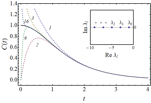
Figure 1: Pseudomode expansion for the toy model. Solid line – exact autocorrelation function (9). Dashed lines – the pseudomode expansion (12) truncated at various orders $l_{\rm max}$ (indicated by numbers). Inset - the pseudomode spectrum of the model.

Pseudomode expansion.  A well-known strategy to improve an approximate solution of a dynamical equation is to add an artificial dissipation and then to consider the limit of the vanishing dissipation strength Mattuck (1992); Rakovszky et al. (2022); White (2023). We implement this idea by introducing diagonal terms

$$a_{n}=\begin{cases}0,&n\leq n_{\rm max}-1\\ i\gamma(n-n_{\rm max}),&n\geq n_{\rm max}\end{cases}$$ (4)

in the evolution superoperator (2), where $\gamma>0$ is the dissipation strength.

There are good reasons to choose this particular form of artificial dissipation. First, any self-adjoint superoperator of Markovian dissipative evolution can be brought to the tridiagonal form (2) Bhattacharya et al. (2022); Bhattacharjee et al. (2023). Second, first $n_{\rm max}$ derivatives of $C(t)$ at $t=0$ remain unaltered by the artificial dissipation (4), thanks to zero diagonal terms. Therefore the artificial dissipation does not alter the initial behavior of the correlation function which is known to be reproduced extremely accurately by the recursion method Uskov and Lychkovskiy (2024).

Finally and most importantly, the linear growth of $a_{n}$ at large $n$ conforms with the dissipative version of the UOGH that is believed to be valid for generic Markovian dissipative systems Bhattacharya et al. (2022); Liu et al. (2023); Bhattacharjee et al. (2023). A remarkable feature of such systems is the localization of eigenvectors of ${\mathcal{L}}$ in the Krylov space Liu et al. (2023) (see also Bhattacharjee et al. (2023), Teretenkov and Lychkovskiy (2024)).

Let us discuss the above localization in more detail. Generically, ${\mathcal{L}}$ is diagonalizable,

$$i\,{\mathcal{L}}\,{\mathcal{U}}={\mathcal{U}}\,\Lambda,$$ (5)

where ${\mathcal{U}}$ is an invertible matrix with column vectors being eigenvectors of ${\mathcal{L}}$, and $\Lambda={\rm diag}(\lambda_{0},\lambda_{1},\lambda_{2},\dots)$ is the diagonal matrix of the corresponding eigenvalues. Since ${\mathcal{L}}={\mathcal{L}}^{\mathsf{T}}$, one can choose ${\mathcal{U}}$ such that ${\mathcal{U}}^{-1}={\mathcal{U}}^{\mathsf{T}}$, which is equivalent to normalizing ${\mathcal{U}}$ according to ${\mathcal{U}}^{\mathsf{T}}{\mathcal{U}}=\mathds{1}$ Teretenkov and Lychkovskiy (2024). We employ such normalization in what follows.

The eigenvalues are either real or come in complex-conjugate pairs. In any case $\operatorname{\mbox{Re}}\lambda_{l}\leq 0$. We order the eigenvalues by the ascending absolute values of their real parts (complex-conjugate pairs $(\lambda_{l},\lambda_{l+1}=\lambda_{l}^{*})$ are additionally ordered according to $\operatorname{\mbox{Im}}\lambda_{l}<0$ ), see Figs. 1,2.

The localization implies that, for any finite $\gamma$,

• the spectrum $\{\lambda_{0},\lambda_{1},\lambda_{2},\dots\}$ of ${\mathcal{L}}$ is discrete and

• the eigenvectors of ${\mathcal{L}}$ are localized, $\big{|}{\mathcal{U}}_{l}^{n}\big{|}<e^{-\kappa|n-l|}$, where $\kappa>0$ is some constant.

Our central set of assumptions that underlie the pseudomode expansion concerns the behavior of $\lambda_{l}$ and ${\mathcal{U}}_{l}^{0}$ in the limit $\gamma\rightarrow+0$ of the vanishing dissipation strength. Namely, we assume that

• $\lim\limits_{\gamma\rightarrow+0}{\mathcal{U}}_{l}^{0}$ exists for all $l$, is bounded in absolute value by a constant independent of $l$ and is nonzero at least for some $l$;

• $\lim\limits_{\gamma\rightarrow+0}\lambda_{l}$ exists and has a strictly negative real part for all $l$;

• the spectrum remains discrete, i.e.

  $$\lim\limits_{\gamma\rightarrow+0}(\lambda_{l}-\lambda_{l^{\prime}}) \neq 0\quad{\rm for}\quad l\neq l^{\prime}.$$ (6)

Note that limiting values of ${\mathcal{U}}_{l}^{n}$ may or may not be localized, as discussed in what follows. The above assumptions will be verified in a toy model of ${\mathcal{L}}$ and in two microscopic spin models, see Figs. 1,2.

After a standard algebra, one obtains $O_{t}={\mathcal{U}}\,e^{\Lambda t}\,{\mathcal{U}}^{\mathsf{T}}O$ and hence

$$C(t)=\sum_{l=0}^{\infty}\big{(}{\mathcal{U}}_{l}^{0}\big{)}^{2}\,e^{\lambda_{l}t}.$$ (7)

In this formula, ${\mathcal{U}}_{l}^{0}$ and $\lambda_{l}$ should be understood as limiting values at $\gamma\rightarrow+0$. We refer to eq.(7) as the pseudomode expansion.

Crucially, thanks to assumption (6), the pseudomode expansion is a discrete sum.

For a nonintegrable many-body system, one is able to accurately compute only a finite number of terms in eq. (7). Fortunately, the pseudomode expansion typically converges very fast, as illustrated by examples below. As a result, the truncated pseudomode expansion containing only a small number $l=l_{\rm max}$ of the terms in the sum (7) can deliver a very good approximation to the actual correlation function. Note that the asymptotic behavior of the autocorrelation function at $t\rightarrow\infty$ is, in general, determined by the leading eigenvalue $\lambda_{0}$ in case of $\operatorname{\mbox{Im}}\lambda_{0}=0$, or by the leading pair of complex conjugate eigenvalues $\lambda_{0}=\lambda_{1}^{*}$ otherwise.

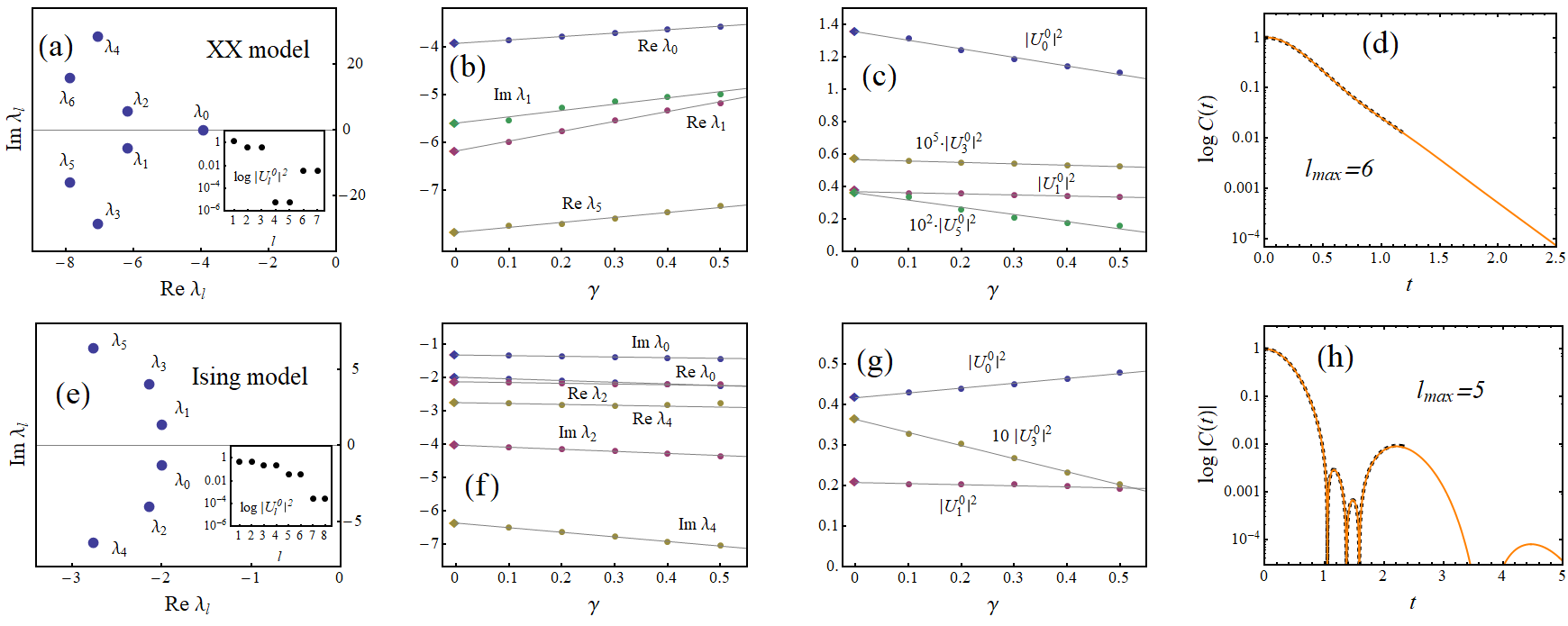
Figure 2: Pseudomode spectra and expansions for two quantum spin-$1/2$ models on a square lattice: upper row – $XX$ model (13), lower row – Ising model (14). (a),(e): The rightmost part of the pseudomode spectrum; the inset shows the pseudomode amplitudes. (b),(f) and (c),(g): The convergence of pseudomode eigenvalues and amplitudes, respectively, in the limit of vanishing dissipation strength $\gamma$. (d),(h): The autocorrelation function $C(t)$ computed by means of the truncated pseudomode expansion (solid orange line, the truncation order $l_{\rm max}$ is indicated in the plot) and with the help of the recursion method Uskov and Lychkovskiy (2024); sup (black dashed line). Note that in the Ising model $C(t)$ has alternating sign, for this reason it is the absolute value of $C(t)$ which is plotted in (h).

Toy model.  Here we consider a toy evolution superoperator Parker et al. (2019); Balasubramanian et al. (2022); Bhattacharjee et al. (2023); sup with

$$b_{n}=\sqrt{1-\gamma^{2}}\,n,\qquad a_{n}=i\gamma(2n+1).$$ (8)

While it is not obtained from any known microscopic many-body model, it is believed to grasp some of the major general features of actual evolution operators, since the sequences of $b_{n}$ and $a_{n}$ follow the UOGH Parker et al. (2019); Bhattacharya et al. (2022); Liu et al. (2023); Bhattacharjee et al. (2023).

Note that coefficients $a_{n}$ in eq. (8) are not exactly of the form (4). The major difference is that they do not vanish for any $n$. The consequence of this fact will be discussed below.

The set (3) of Heisenberg equations for this toy ${\mathcal{L}}$ can be explicitly solved with the result Parker et al. (2019); Balasubramanian et al. (2022); Bhattacharjee et al. (2023); sup

$$C(t)=\frac{1}{\cosh(t)\,(1+\gamma\tanh(t))}~{}\xrightarrow{\gamma\rightarrow 0}~{}\frac{1}{\cosh(t)}.$$ (9)

Our goal is to reproduce this autocorrelation function by means of the pseudomode expansion (7).

This task can be easily completed since the spectrum and the eigenvectors of ${\mathcal{L}}$ can be explicitly computed for $\gamma\in(0,1)$ Parker et al. (2019); Balasubramanian et al. (2022); Bhattacharjee et al. (2023); sup :

$$\lambda_{l} =-(2l+1),$$ (10)

$${\mathcal{U}}_{l}^{0} =\sqrt{\frac{2}{1+\gamma}}\,(-i)^{l}\left(\frac{1-\gamma}{1+\gamma}\right)^{l/2}\,\xrightarrow{\gamma\rightarrow+0}\sqrt{2}\,(-i)^{l}.$$ (11)

All eigenvalues are real negative and do not depend on $\gamma$, while ${\mathcal{U}}_{l}^{0}$ have a finite limit of vanishing dissipation strength. Hence our assumptions are satisfied and the pseudomode expansion (7) reads

$$C(t) =2\sum_{l=0}^{\infty}(-1)^{l}\,e^{-(2l+1)t}.$$ (12)

Remarkably, the eigenvectors (11) exhibit localization for any finite $\gamma$ (see sup for details) but not in the limit of vanishing $\gamma$. Still, the sum in eq. (12) converges for any fixed $t>0$, thanks to the linear growth of $\lambda_{l}$ with $l$. This is illustrated in Fig. 1, where the truncated pseudomode expansion is compared to the actual value of $C(t)$ for various truncation orders $l_{\rm max}$. One can see that the convergence is spectacular at intermediate and large times. In particular, the leading pseudomode correctly reproduces the asymptotic behavior $C(t)\sim 2e^{-t}$ at large times. However, the convergence worsens at small times and is absent at $t=0$. This is not surprising, since the small-time behavior is expected to be reproduced provided coefficients $a_{n}$ vanish for first few $n$, which is not the case in this toy model.

Spin models.  Here we consider two spin-$1/2$ models on the square lattice. The first one is the $XX$ nearest-neighbour model with the Hamiltonian

$$H_{XX}=\sum_{\langle{\mathbf{i}}{\mathbf{j}}\rangle}(\sigma^{x}_{{\mathbf{i}}}\sigma^{x}_{{\mathbf{j}}}+\sigma^{y}_{{\mathbf{i}}}\sigma^{y}_{{\mathbf{j}}}),$$ (13)

where ${\mathbf{i}}$ and ${\mathbf{j}}$ label lattice sites and the sum runs over pairs of neighbouring sites. The second model is the transverse field Ising model with the Hamiltonian

$$H_{\rm Ising}=\sum_{\langle{\mathbf{i}}{\mathbf{j}}\rangle}\sigma^{x}_{{\mathbf{i}}}\sigma^{x}_{{\mathbf{j}}}+\sum_{{\mathbf{j}}}\sigma^{z}_{{\mathbf{j}}}.$$ (14)

For both models we choose the observable

$$A=\sum_{\begin{subarray}{c}~{}\,\langle{\mathbf{i}}{\mathbf{j}}\rangle_{-}\\ {\mathbf{i}}\prec\,{\mathbf{j}}\end{subarray}}(\sigma^{x}_{{\mathbf{i}}}\sigma^{y}_{{\mathbf{j}}}-\sigma^{x}_{{\mathbf{j}}}\sigma^{y}_{{\mathbf{i}}}),$$ (15)

where the sum runs over horizontal bonds, the site ${\mathbf{i}}$ being always to the left of the site ${\mathbf{j}}$. Up to multiplicative constants, this observable has the meaning of the spin current for the $XX$ model and the energy current for the Ising model.

We are able to explicitly compute $n_{\rm max}=11$ Lanczos coefficients $b_{n}$ for the $XX$ model sup and $n_{\rm max}=21$ – for the Ising model Uskov and Lychkovskiy (2024). For larger $n$, coefficients $b_{n}$ are extrapolated linearly in accordance to the UOGH. The coefficients $a_{n}$ are chosen according to eq. (4) with some $\gamma$. After that, the infinite matrix ${\mathcal{L}}$ is truncated at some large size $k$ (we find appropriate to take $k=2000$) and diagonalized numerically. As a result, we obtain the pseudomode eigenvalues $\lambda_{l}$ and amplitudes $\big{(}{\mathcal{U}}_{l}^{0}\big{)}^{2}$ for the chosen value of $\gamma$.

The scaling of the pseudomode eigenvalues and amplitudes in the limit of vanishing $\gamma$ is shown in Fig. 2 (b),(c),(f),(g). One can see that all our assumptions underlying the pseudomode expansion are confirmed.

The pseudomode spectra for the two models under consideration are shown in Fig. 2 (a) and (e). The major difference between the two is that the $XX$ model has a real leading eigenvalue $\lambda_{0}$ which entails a pure exponential decay at large times, while the Ising model has a complex-conjugate pair $(\lambda_{0},\lambda_{1})$ of the leading eigenvalues which leads to oscillations superimposed on the exponential decay, see Fig. 1 (d) and (h).

Remarkably, in contrast to the toy model, here the localization of eigenvectors survives the limit of vanishing coupling, and pseudomode amplitudes $\big{(}{\mathcal{U}}_{l}^{0}\big{)}^{2}$ decay exponentially with $l$, as can be seen from insets in Fig. 2 (a),(e). This dramatically increases the rate of convergence of the pseudomode expansion. In fact, it turns out that a correlation function can be accurately approximated by a sum of only a few first pseudomodes, as illustrated in Fig. 2 (d),(h).

Summary and outlook.  To summarize, our studies confirm a long-standing surmise Fine (2004, 2005) that a time-dependent correlation function of a generic many-body system can be accurately approximated by a linear combination of a few pseudomodes $e^{\lambda_{l}t}$ with complex eigenvalues $\lambda_{l}$. We have presented an algorithmic way to compute pseudomode eigenvalues and amplitudes starting from the Lanczos coefficients obtained within the recursion method. While previous implementations of the recursion method have been able to access only finite, although often appreciably large, time scales Thomas et al. (2023); Wang et al. (2023); Bartsch et al. (2023); Uskov and Lychkovskiy (2024), the pseudomode expansion recovers the correlation function at all times, including the asymptotic behavior.

It would be interesting to explore methods to compute the pseudomode expansion other than the recursion method. This may be particular relevant beyond the infinite-temperature case studied in the present paper, since computing Lanczos coefficients at finite temperatures remains a largely unaddressed problem.

Finally, an intriguing open question is whether one can give more physical meaning to pseudomodes, e.g. interpret them as quasiparticles with a finite lifetime.

Appendix A Supplementary material

Appendix B S1. Toy model

The toy evolution operator (2),(8) can be represented as

$${\mathcal{L}}=i\gamma M+\sqrt{1-\gamma^{2}}(B+B^{\dagger}),$$ (S1)

where

$$M=\begin{pmatrix}1&0&0&0&\dots\\[3.00003pt] 0&3&0&0&\dots\\[3.00003pt] 0&0&5&0&\dots\\[3.00003pt] 0&0&0&7&\dots\\[3.00003pt] \vdots&\vdots&\vdots&\vdots&\ddots\end{pmatrix},\qquad B=\begin{pmatrix}0&1&0&0&\dots\\[3.00003pt] 0&0&2&0&\dots\\[3.00003pt] 0&0&0&3&\dots\\[3.00003pt] 0&0&0&0&\dots\\[3.00003pt] \vdots&\vdots&\vdots&\vdots&\ddots\end{pmatrix}.$$ (S2)

Crucially, operators $M$ and $B$ satisfy

$$[B,B^{\dagger}]=M,\qquad[B,M]=2B,\qquad[B^{\dagger},M]=-2B^{\dagger},$$ (S3)

cf. ref. Accardi et al. (2002). These commutation relations can be easily obtained from the action of the above operators on basis vectors $|n\rangle$, $n=0,1,2,\dots$:

$$B|n\rangle=n|n-1\rangle,\quad B^{\dagger}|n\rangle=(n+1)|n+1\rangle,\quad M|n\rangle=(2n+1)|n\rangle.$$ (S4)

Using commutation relations (S3), one brings ${\mathcal{L}}$ to the diagonal form as follows:

$${\mathcal{L}}=e^{i\tau(\gamma)(B^{\dagger}-B)}(iM)e^{-i\tau(\gamma)(B^{\dagger}-B)},$$ (S5)

where

$$\tau(\gamma)=\arccos\left(-\sqrt{\frac{1+\gamma}{2}}\right),\quad\gamma\in(0,1).$$ (S6)

Thus ${\mathcal{U}}$ and $\Lambda$ from eq. (5) read

$${\mathcal{U}}=e^{i\tau(\gamma)(B^{\dagger}-B)},\qquad\Lambda=-M.$$ (S7)

Eigenvalues (10) follow immediately. Eigenvectors (11) and autocorrelation function (9) are obtained after some straightforward algebra.

Appendix C S2. Recursion method for the $XX$ model on the square lattice

The implementation of the recursion method with the symbolic calculation of nested commutators and the extrapolation of Lanczos coefficients according to the UOGH is described in ref. Uskov and Lychkovskiy (2024). There, in particular, the autocorrelation function for the Ising model is computed. We follow the same procedure to compute the autocorrelation function of the $XX$ model. To this end we compute $n_{\rm max}=11$ nested commutators and the same number of moments $\mu_{n}$ shown in Table 1. The Lanczos coefficients are obtained from the moments as described in ref. Viswanath and Müller (2008).

$n$	$\mu_{n}$
1	16
2	1024
3	136192
4	30277632
5	9983098880
6	4498943967232
7	2599858319392768
8	1834298158063026176
9	1527776305296896425984
10	1472244134830457072123904
11	1624011303835553036301762560

Table 1: Moments for the Hamiltonian (13) and observable (15).