Planar reinforced -out percolation
Abstract.
We investigate the percolation properties of a planar reinforced network model. In this model, at every time step, every vertex chooses incident edges, whose weight is then increased by 1. The choice of this -tuple occurs proportionally to the product of the corresponding edge weights raised to some power .
Our investigations are guided by the conjecture that the set of infinitely reinforced edges percolates for and . First, we study the case , where we show the percolation for after adding arbitrarily sparse independent sprinkling and also allowing dual connectivities. We also derive a finite-size criterion for percolation without sprinkling. Then, we extend this finite-size criterion to the case. Finally, we verify these conditions numerically.
1. Introduction
Mathematical processes with reinforcements are a vibrant research field as they appear in a wide range of applications. For instance, in economics, dominant companies that already have a large market share are more likely to expand their share even further. In neuroscience, synapses that have been used successfully in the past are more likely to be strengthened in the future. This effect, known as neuroplasticity, is the reason for a dynamical evolution of the neural network. An extreme form has been suggested by Markram et al. as tabula-rasa hypothesis [15].
The challenge for mathematicians is to explain how local reinforcement mechanisms drive global network properties. This has initiated the novel research field of graph-based reinforcement models. Here, we address the question whether it is possible to design a reinforcement mechanism that gives rise to a network structure that is sparse but can still connect distant areas in the brain.
In this work, we propose a percolating model of graph-based reinforcement, which is based on the idea of -out networks. The evolution of the network takes place in rounds. In each round, each vertex reinforces precisely of its incident edges. The selection of such a -tuple is proportional to the product of the current edge weights raised to some reinforcement parameter . A particularly important special setting is the case where , where even a small weight difference makes an edge infinitely stronger than another one with lower weight.
The question of percolation of the infinitely-reinforced edges is the main focus of our interest. More specifically, we concentrate on the case . Here, our overarching conjecture is that percolation occurs once is sufficiently large. Our main result, Theorem 3 below, is a major step towards this conjecture in the case . More precisely, we show that there is percolation after an arbitrarily sparse sprinkling of independent open edges when using a modified notion of connectivity that will be specified precisely below. Moreover, we provide several rigorously proven finite-range criteria for percolation, for which we then obtain overwhelming numerical evidence by Monte Carlo simulation. All of these results are stated in full detail in Section 2 below.
We conclude the present introduction by elaborating on the connections of our work to two vibrant fields of research, namely i) graph-based reinforcement, and ii) dependent models for percolation, especially those violating the FKG condition.
Graph-based reinforcement. Pioneering works in the area of graph-based reinforcment are [4, 6] where the reinforcement is set on the vertices of the graph. In the context of neuroscience, it is more natural to consider edge-based reinforcement, and those were introduced in the seminal work [13]. One of the major drawback of this model is that even for , it does not give rise to percolating structures [11]. Percolation could be achieved when relying on tree-based models [9, 10]. However, this imposes already very strong a priori structures. An interesting alternative form of graph reinforcement comes from ant-based walks [16, 17].
Percolation without FKG. In recent years, the investigation of dependent percolation models has attracted considerable attention. We refer the reader to [8] and references therein. However, although a broad range of models has been considered, the vast majority satisfies the FKG inequality, i.e., positive correlation of increasing events. When considering questions beyond the validity of the FKG inequality, only a few isolated results are available. The results treated in [12, 18] fundamentally rely on the Gaussian field and Poisson point process setting, respectively, and therefore do not apply in our setting. To solve this problem in our setting, we develop a completely novel stochastic domination property.
While our investigation concern a reinforced model for -out percolation, we stress here that already the question of independent -out percolation has been the topic of vigorous research. More precisely, to put our investigation into perspective, we first review the independent -out model discussed in [14]. Here, at each site , we select independently and uniformly at random a -element subset of all bonds incident at . We let denote the random graph obtained as the union of all these bonds. Then, we let
denote the smallest value of such that percolates, noting that . A key property of this model is the negative correlation of the vacant edges.
Proposition 1 (Percolation of independent -out percolation on ; [14]).
For every , we have that . Moreover, .
The rest of the manuscript is organized as follows. In Section 2, we give a detailed description of our -out percolation model and state all our main results. Section 3 contains the proof of a crucial domination property. In Section 4, we prove a sprinkling result by establishing sharp phase transition and combining it with the domination result. Subsequently, in Section 5, we derive certain finite-size criteria for percolation, for which we then present overwhelming numerical evidence in Section 6.
2. Model and main results
In this work, we consider a reinforced model for -out percolation, which depends on a reinforcement parameter . First, in Section 2.1, we focus on the case . Then, in Section 2.2, we consider the setting of finite .
2.1. The case
In this model, we assign weights to the edges of the hyper-cubic lattice , which evolve in discrete time steps. Initially, all edges have weight . Then, at every discrete time the weights are updated as follows.
-
(1)
At every site , we select one tuple , where denote the family of -tuples of edges incident to . More precisely, we order all adjacent edges according to their momentary weights in decreasing order (breaking ties by independent coin flips). We set to be the first of these edges in this decreasing order.
-
(2)
The weight of each edge is then increased by the number of times it was selected. This selection is done simultaneously for all vertices based on the weights . As it can happen that an edge is selected by each of its two endpoints, one has .
This results in the “final” configuration
| (1) |
of edges that are eventually reinforced in every round. Our arguments in Section 3 show that this set coincides with the set of edges that are reinforced infinitely often. The same set of arguments shows that our percolation model is stochastically dominated by the independent -out model mentioned in Proposition 1. This is explained in the proof of Proposition 7 below.
To simplify the terminology, we call an edge open if and closed otherwise. As elucidated in the introduction, we hypothesize that percolates for . That is, we make the following conjecture.
Conjecture 2 (Percolation for ).
Assume that . Then,
The aim of this work is to present a series of results supporting this core conjecture. First, superpose the edges of interest it with some sprinkling, i.e., by adding an independent Bernoulli percolation process with some small parameter . We write for the sprinkled set of bonds and put . Adding the sprinkled bonds makes it substantially easier to find an infinite connected component. One of the striking properties of planar Bernoulli bond percolation is its self-duality. While our dependent model is still planar, it is no longer self-dual. This means that when applying classical techniques from percolation theory, the implications are often different than in Bernoulli bond percolation. However, for our argument to work, we still need to allow the alternative that there is an infinite component where the adjacency notation from the original lattice is replaced by the adjacencies from the dual lattice. That is, two edges of are dually adjacent if there exists such that contains both edges.
We say that the model percolates if there exists an infinite sequence of distinct edges in such that for all , we have that and are adjacent. We further say that the model percolates dually if there exists an infinite sequence of distinct edges in such that for all , we have that and are dually adjacent.
Theorem 3 (Percolation of sprinkled percolation).
Let and . Then,
The proof of Theorem 3 relies fundamentally on the OSSS inequality from [19]. In order to apply it, we need to derive bounds on influences and revealment probabilities. Here, we note that the influences are intimately related to probabilities of pivotal events, which have been studied for the geometrically challenging models such as Voronoi percolation [7]. However, the arguments of [7] heavily rely on the FKG inequality, which is not available for our model. While recently, there has been progress in applying the OSSS inequality in models without FKG inequality [12, 18], these arguments are highly model dependent and do not extend to the present setting. We will address this challenge through a completely novel stochastic domination property in our setting, see Proposition 7 below. It is when extending the techniques of [12, 18] to our model that the finite range of dependance will be crucial.
Conjecture 2 is a percolation result for a model with parameter , which is similar to the continuous model considered in [1]. Here points of a Poisson point process are connected to their nearest neighbors. To study this percolation process, the authors develop a rigorous finite-size criterion, which is then verified “with high probability” through a simulation.
We next aim to transfer this finite-size approach to our situation, similar adaptation were considered in [2, 5]. The key idea is to identify edges , where it is already possible to say after a finite number of rounds whether . More precisely, an edge is after rounds
-
(1)
certainly vacant if it is reinforced at most times;
-
(2)
potentially occupied if it is reinforced precisely times;
-
(3)
certainly occupied if it is reinforced at least times. Moreover, if a node is incident to two certainly vacant edges, then the remaining two edges are also -certainly occupied.
The reason for this terminology is that as shown in the proof of Lemma 8, if an edge is certainly occupied, then it is eventually reinforced in every round. Similarly, if an edge is certainly vacant, it is only reinforced a finite number of times.
Now, we say that the rectangle is -open if there exist three types of crossings of the central rectangle with edges that are certainly occupied after rounds:
-
(1)
a horizontal crossing of the -rectangle;
-
(2)
vertical crossings of the left and right -squares in the central rectangle.
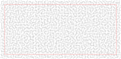
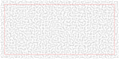
Figure 1 shows the crossings of the central rectangle. There is no particular conceptual reason for the values 80 and 40. However, we found them to be convenient for the simulations in Section 6. Henceforth, we often think of the -rectangle as being a horizontal edge in a coarse-grained lattice.
Having introduced the notion of -openness, we define as the event that the coarse-grained edges is -open. Then, we show that if , then . The deeper reason behind the value 0.8457 is the recent paper [3, Theorem 1], which shows that any 1-dependent 2D bond percolation model percolates if the marginal probability exceeds this value.
Theorem 4 (Finite-size criterion).
Let and be such that . Then,
Using Monte Carlo simulation, we show that with a certainty exceeding , the finite-size crossing probability in Theorem 4 indeed exceeds the threshold 0.8457 of 1-dependent percolation.
2.2. The case
Next, we deal with the case . We go through the algorithm for the weight evolution similarly as in the case where and again initialize the weights with for every . Then, for each , we carry out the following updates
-
(1)
At every site , we select one tuple whose edge weights are increased by 1.
-
(2)
These edges are selected with probability proportional to .
In the limiting case , we recover the simplified reinforcement mechanism discussed above. Therefore, it is plausible to extend Conjecture 2 from to the case of large but finite .
Conjecture 5 (Percolation of reinforced 2-out percolation on ; finite ).
Assume that . Then, there exists such that whenever .
As before, we add independent sprinkling on the edges with a sprinkling probability . As in the case of , we consider then the union of edges that are reinforced infinitely often together with the sprinkled edges.
Ideally, as a first step, we would like to present a finite-size criterion as in Theorem 4. The key difficulty is that now, it is more complicated to identify edges where we know that they will be reinforced either finitely or infinitely often. For instance, if an edge has weight 1 after 10 rounds, it could still happen (although extremely unlikely) that it will still be reinforced in each of the following 100 rounds.
Hence, we need to introduce a process of corrupted vertices to take into account such effects. More precisely, let be a fixed (small) corruption probability. Then, each vertex incident to at least one edge of weight at most after rounds is declared -corrupted independently with probability . Having introduced the corrupted vertices, we can now extend the concept of certainly occupied edges. More precisely, after rounds, we say that an edge that is not incident to a corrupted vertex is
-
•
certainly vacant if it is reinforced at most times;
-
•
certainly occupied if it is not certainly vacant and is incident to a node which itself is incident to two certainly vacant edges.
To introduce the finite-size criterion, we now proceed in the same way as in . Again, to avoid boundary effects, we consider a central rectangle rectangle with edges that are certainly occupied after rounds. Then, we say again that it is -open if there exist the three types of crossings considered in the case . Now, we say that a horizontal edge between and is -open if the rectangle has this property in the above sense. Similarly, we define the openness of vertical edges. Now, we let denote the event that the coarse-grained edges is -open with corruption probability set as
| (2) |
We note that the infinite sum cannot be evaluated in closed forms. However, it would be possible to present closed-form bounds through suitable integral bounds. For fixed , we can (and will) choose so that is sufficiently small.
Theorem 6 (Percolation of reinforced 2-out percolation on ).
Let . Furthermore, assume that and are such that . Then, .
We note that the bound on is the result of a comparison with a strongly-reinforced Pólya urn process, which we elaborate on in Lemma 14 below. Again, in Section 6, we provide overwhelming evidence from Monte Carlo simulations that .
Finally, we stress again that the difficulty of analyzing the reinforced model is that it exhibits long-range dependencies and does not satisfy the FKG inequality. This means that the vast majority of the standard percolation arguments break down for this model. Nevertheless, in the case , the model enjoys the following intriguing domination property.
Proposition 7 (Domination of when ).
If , then the random set stochastically dominates .
It is unclear if the stochastic-domination property also holds for . However, we believe that an analog of Proposition 7 could be possible for a clever choice of finite reinforcement function.
3. Proof of Proposition 7
We will describe a new colored process, equivalent to our original reinforcement process for , from which the derivation of Proposition 7 will be straightforward. In this colored process, each edge has a blue counter and a red counter that increase with time. At the beginning we set for all edges.
At each step, every vertex chooses of its adjacent edges, which increase their blue counter by , and the other two increase their red counter by . The choice is made according to the same reinforcement mechanism as in our regular process — we choose the edges incident to with the highest value to increase theis blue counter while all the other incident edges increase their red counter, breaking ties by choosing uniformly at random. Set
Finally set
We make the following simple observations:
Lemma 8.
-
(1)
For every edge and every , .
-
(2)
For every , it holds that , where means that the union is disjoint.
-
(3)
are increasing sequences, is decreasing.
-
(4)
.
-
(5)
and have the same distribution, and have the same distribution.
-
(6)
, .
Before proving Lemma 8, we explain how to deduce Proposition 7, where the main step will be to identify the models in such a way that . This identification also gives that , which implies that our model is stochastically dominated by the independent -out model with .
Proof of Proposition 7.
The connection to our reinforcement model comes by looking only at the blue counters. Under this identification we get that is the set of all certainly occupied edges and is the set of certainly vacant edges at time . Also . The claim now follows directly from clause of Lemma 8. ∎
Now, we give the proof of Lemma 8.
Proof of Lemma 8.
-
(1)
The assertion follows from the fact that each edge gets either a red counter or a blue counter from each of its endpoints.
-
(2)
Clause implies that are a disjoint partition of .
-
(3)
We will show this for , and follows by symmetry. Take some edge and consider the first time for which . Then at time , the edge got a blue counter from both its endpoints. Therefore, was among the largest blue counters of edges incident to (and similarly for ). Moreover, the blue counter of any edge can increase by at most at every step. Therefore, is strictly larger than the lowest blue counters of edges incident to . As a consequence, the edge will keep being chosen by both and for all rounds . This implies that for all . Finally, the fact that is decreasing now follows from clause .
-
(4)
Clause implies that the unions defining and are increasing, and that the intersection defining is decreasing. Therefore, the statement follows from clause .
-
(5)
By clause , choosing the edges with the highest blue counter is the same as not choosing those with the highest red counter. This makes the definition of the process symmetric w.r.t. flipping the colors.
-
(6)
This follows from a similar argument to the monotonicity clause .
∎
4. Proof of Theorem 3
In this section, we prove Theorem 3. That is, we show that percolation occurs in the dual or original lattice after adding arbitrarily sparse independent sprinkling. In (1), we defined the set of edges that are eventually reinforced in every round. One challenge of dealing with this set is that it has an unbounded range of dependencies. To overcome this difficulty, we now introduce an approximated version of the set after a finite number of rounds. We say that an edge is -potentially occupied (and write ) given the configuration after rounds if it is still possible with positive probability that . Further, we call an edge strictly -potentially occupied if . The main idea is to show percolation for each of the approximated sets and then to use a stochastic domination result to control the difference .
This strategy is similar to that used in [7], where the authors prove a similar result for Voronoi percolation. The key similarity is that both Voronoi percolation and our model are spatial percolation models with exponential decay of correlations.
To summarize, the proof of Theorem 3 relies on two central results, namely Propositions 9 and 10 below.
Proposition 9 (Sharp threshold for approximation).
Fix and let denote the critical sprinkling probability in the -approximated model. Then, for , the diameter of the clusters has exponentially decaying tails.
Let denote the collection of sites that are incident to at least one edge that is strictly -potentially occupied.
Proposition 10 (Stochastic domination).
Let . Then, is dominated by a Bernoulli site percolation process with marginal probability .
We first discuss how to prove Theorem 3 subject to the validity of Propositions 9 and 10. Then, we prove these propositions in the subsequent subsections.
Proof of Theorem 3.
Proposition 10 gives a stochastic domination of by a Bernoulli site percolation process with marginal probability . We first claim that from this result, we can conclude that the edges incident to sites in are stochastically dominated by a Bernoulli bond percolation process with probability . Indeed, consider an arbitrary finite edge set . Let denote the set of left or lower endpoints of the edges in . Then, by Proposition 10,
thereby proving the claimed stochastic domination. A consequence is that provided that is so large that . We also note that the independent superposition of two Bernoulli bond percolation processes with parameter is again a Bernoulli bond percolation process, whose parameter is then .
Now, to derive a contradiction, assume that for some
Then, Proposition 10 implies that,
In other words, is a subcritical sprinkling probability both with respect to original and dual connectivities of the -approximated model. In particular, is in the strictly subcritical regime, where Proposition 9 guarantees the exponential tail decay of the cluster sizes. In particular, by Proposition 9, both the sizes of the clusters with respect to the original connectivities and with respect to the dual connectivities have exponentially decaying tails. Consequently, the probability to have left-right vacant crossings of large squares tends to 1 as the side length of the square tends to infinity.
Now, by Proposition 7, the occupied edges dominate the vacant ones in , thereby contradicting the exponential decay of the cluster sizes. ∎
We will prove Propositions 9 and 10 in Sections 4.1 and 4.2 below. For both results, it is convenient to describe more precisely how our model can be constructed as a factor of a model with independent inputs. First, we introduce an iid sequence that encodes the sprinkling of edges. More precisely, each is uniformly distributed in and the set of sprinkled edges is then given by
Second, we attach to each site a sequence of iid decision variables . All variables are independent for different values of and also independent of the sprinkling variables .
Given the configuration of edge reinforcements up to iteration , the variable is used to decide which of the edges are reinforced by in iteration . We write
for the sequence of all decision variables at . Then, we write for the collection of all . Hence, the entire randomness of the model can be encoded in the pair
4.1. Proof of sharp thresholds for approximation – Proposition 9
We will deduce Proposition 9 from a differential inequality in the spirit of [8, Lemma 1.7]. We also write for the probability that in the sprinkled model the connected percolation component of the origin has -diameter exceeding , which we denote as .
Proposition 11 (Differential inequality).
There exists such that for every and we have
Applying the OSSS inequality (after O’Donnell, Saks, Schramm and Servedio, [19]) to an algorithm determining gives that
| (3) |
where
-
(i)
is the probability that the algorithm reveals the value of , and
-
(ii)
denotes the (resampling) influence, where is the percolation event after replacing the randomness at by an independent copy, while leaving fixed.
The quantities and are defined similarly. Henceforth, we rely on a specific algorithm from [8], which involves an additional randomization through a uniform integer . For the convenience of the reader, and to make the manuscript self-contained, we briefly recall the idea behind this algorithm. The idea is to explore the clusters by starting from . More precisely, we proceed as follows:
-
(1)
Reveal the value of for all edges incident to . Also reveal for all at -distance at most from a point in .
-
(2)
Suppose that the values of and of have already been revealed at the start of iteration of the algorithm. Let be the union of all connected components that are revealed by this iteration. Then, according to some arbitrary rule, we pick out some unrevealed site that is incident to an edge in . We then reveal the values of for any edge adjacent to . We also reveal the values of for all at -distance at most from .
The proof of Proposition 11 relies on the following two central auxiliary results (Lemmas 12 and 13 below) concerning a comparison of the two influences, and a bound on the revealment probabilities, respectively.
Lemma 12 (Comparison of influences).
Let . Then, there is such that for every ,
Lemma 13 (Bound on revealment probabilities).
Let . Then, there is with the following property. Let the randomized algorithm starting the exploration from , with uniform in . Then,
Proof of Proposition 11.
Hence, we now prove the auxiliary results Lemmas 12 and 13, starting with Lemma 12. The idea is similar to [7], where a comparison between different forms of pivotality also plays a crucial role. However, our situation is a bit simpler in the sense that -approximated model has the bounded dependence range .
Proof of Lemma 12.
For , we introduce the event
where denotes the configuration obtained from by setting for every .
Now, using that the -approximated model has dependence range , we see that if the resampling of at changes the value of , then must occur. In other words, . Hence, it suffices to relate the probability of with the sum of the influences for .
To achieve this goal, we write for the configuration of the model with the sprinkled edges replaced by independent copies for every . Then, we let denote the event that in none of the edges in is sprinkled. We also let denote the event that in the resampled configuration all edges in are sprinkled. Then, by independence and the definition of , we have
for some . Noting that the right-hand side is bounded above by concludes the proof. ∎
Hence, it remains to establish the revealment bounds asserted in Lemma 13. Here, we proceed similarly as in [8], noting that again the finite-range property of our model simplifies the argument.
Proof of Lemma 13.
We only bound the revealment probability , as the bound on is easier. The key observation is that if the randomized algorithm starts from exploring with for some , then the following holds. If reveals the state of for some site , then . Therefore,
where we use the convention for . Thus, picking uniformly at random, we obtain that
for a suitable . This concludes the proof. ∎
4.2. Proof of stochastic domination of approximation – Proposition 10
To prove Proposition 10, we need to describe more precisely how the decision variables determine the state of the edges.
Proof of Proposition 10.
Our construction depends on the parity of , and we first discuss the case of odd . Henceforth, we implicitly consider to be endowed with a checkerboard pattern so that we can speak of black and white sites.
For a black site , we let encode in some arbitrary way a random selection of two of the highest-weight edges incident to . Next, to determine the reinforcements at a white site , we work conditioned on the edge weights up to iteration and also on the decision variables for all black sites . We note that the probability space of selecting two highest-weight edges incident to consists of elements.
First, consider the case where, in step , at least 2 of the black neighbors of reinforced their corresponding edge to the white vertex . Then, there is a probability of at least that, in step , the vertex selects the same two edges, which are therefore reinforced infinitely often, see clause (3) in Lemma 8.
Second, consider the case when there are at least 2 neighboring black vertices of that did not reinforce their corresponding edge to the white vertex . Then, again with probability of at least , in step , the vertex selects the other two edges. Then, again by Lemma 8, these two edges are never reinforced again. Therefore, the vertex is no longer incident to any strictly -potentially occupied edges.
Writing for the collection of decision variables of all sites up to step together with the decision variables at the black sites at step , we conclude that there exists a state such that almost surely, i) and ii) if , then after step , all potentially reinforced edges incident to are in fact reinforced infinitely often.
Taking into account these observations, we now present a two-step construction of the variables . For this, let be an iid sequence of Bernoulli random variables with parameter . If , then we let be the state . Otherwise, if , then we let be the state with probability , and with probability the random variable is sampled according to the conditional distribution .
This describes the construction for odd steps . For even , we proceed in precisely the same manner except that the roles of black and white sites are interchanged. In particular, if an edge incident to a black site is contained in , then . This proves the asserted domination. ∎
5. Proofs of Theorems 4 and 6
We deal separately with the cases and . We start with , where we use a result for 1-dependent percolation with sufficiently high marginal probabilities from [3]. We apply this result to the coarse-grained model. The key observation is that if the coarse-grained edge is -open, then we are guaranteed three crossings of infinitely-reinforced edges in the rectangle . Namely,
-
(1)
a horizontal crossing of the -rectangle;
-
(2)
vertical crossings of the left and of the right -squares inside the central rectangle.
Moreover, the existence of such crossings depends only on coarse-grained edges sharing at least one of the end points. Hence, we conclude from planarity that any path of -open coarse grained edges gives rise to a path of infinitely-reinforced edges. Hence, it suffices to establish the percolation of the coarse-grained model, which we do now.
Proof of Theorem 4; .
The collection of -open edges defines a 1-dependent family. Now, by our assumption on the finite-size criterion, a coarse-grained edge is open with marginal probability exceeding 0.8457. Now, we can conclude the proof by invoking [3, Theorem 1], which states that any 1-dependent site percolation model with marginal probability exceeding 0.8457 percolates. ∎
We now turn to the case . We first argue that percolation of the -open edges in the coarse-grained model implies percolation of the infinitely-reinforced model in the original model.
Lemma 14 (Stochastic domination property of certainly occupied edges).
Let and assume
Then, the process of edges that are reinforced only finitely often in the original model is stochastically dominated by the process of edges that are not certainly occupied.
Proof.
The idea of the proof is as follows. If after rounds an edge has weight at most , then for large , it is highly likely never to be chosen again. Then, loosely speaking, the vertex corruption is used to account for the possibility of this exceptional event.
To make this precise, we let denote the event that the edge with weight at most in round is reinforced by at least one of its incident vertices in some round . Then, we claim that is stochastically dominated by a directed Bernoulli bond percolation process with probability . To achieve this goal, we note that at the beginning of round there are at least 2 high-weight edges, i.e., edges of weight at least . Hence, the probability that one of the low-weight edges is reinforced from one of its incident vertices is at most
We stress that this upper bound holds irrespective of the weight evolution at any of the other directed edges. Hence, the union bound shows that, as asserted, the edge process is dominated by a Bernoulli bond process with probability . ∎
Proof of Theorem 4; .
After the reduction step from Lemma 14, the proof is very similar to that in the case . Arguing as in the case , Lemma 14 guarantees that any path of -open coarse grained edges gives rise to a path of infinitely-reinforced edges. Moreover, we conclude from the condition (2) that the probability for a coarse-grained edge to be -open exceeds 0.8457. The theorem then follows, as for , by invoking [3, Theorem 1]. ∎
6. Numerical evidence for the finite-size criteria
We start with Theorem 4, i.e., where . Here, we carried out simulations of the process in a -rectangle with periodic boundary conditions. In of these simulations we found a horizontal crossing of the central -rectangle of the nodes that are certainly occupied after steps. Using that the Monte Carlo variance is , this implies that with a certainty exceeding , the actual crossing probability is above the threshold of for 1-dependent percolation The simulations took 22min 17s on a 13th Gen Intel Core i5-1345U. Figure 2 illustrates examples for crossing and non-crossing realizations.
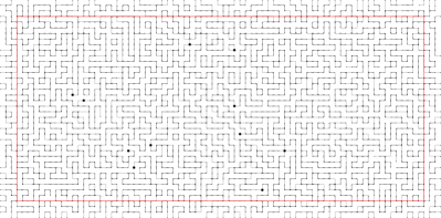
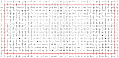
Finally, we discuss Theorem 6, i.e., where . Our simulations concern . The basic setting is the same as above, namely simulations on a -rectangle with periodic boundary conditions. In of these simulations we found percolation of the central -rectangle of the nodes that are certainly occupied after steps. Again, with a certainty exceeding , the actual crossing probability is above the threshold of for 1-dependent percolation. The simulations took 1h 42min 52s on a 13th Gen Intel Core i5-1345U. Note that additional time is needed for sampling from a discrete probability distribution and for dealing with the corruption. Figure 3 illustrates examples for crossing and non-crossing realizations.
Acknowledgments
This work was initiated during the workshop Adaptive Learning and Opinion Dynamics in Social Networks at Bar-Ilan University in Tel Aviv.
References
- [1] P. Balister, B. Bollobás, A. Sarkar, and M. Walters. Connectivity of random k-nearest-neighbour graphs. Advances in Applied Probability, 37(1):1–24, 2005.
- [2] P. Balister, B. Bollobás, and M. Walters. Continuum percolation with steps in the square or the disc. Random Structures Algorithms, 26(4):392–403, 2005.
- [3] P. Balister, T. Johnston, M. Savery, and A. Scott. Improved bounds for 1-independent percolation on . arXiv preprint arXiv:2206.12335, 2022.
- [4] M. Benaïm, I. Benjamini, J. Chen, and Y. Lima. A generalized Pólya’s urn with graph based interactions. Random Structures Algorithms, 46(4):614–634, 2015.
- [5] B. Bollabás and A. Stacey. Approximate upper bounds for the critical probability of oriented percolation in two dimensions based on rapidly mixing Markov chains. J. Appl. Probab., 34(4):859–867, 1997.
- [6] J. Chen and C. Lucas. A generalized Pólya’s urn with graph based interactions: convergence at linearity. Electron. Commun. Probab., 19:no. 67, 13, 2014.
- [7] B. Dembin and F. Severo. Supercritical sharpness for Voronoi percolation. arXiv preprint arXiv:2311.00555, 2023.
- [8] H. Duminil-Copin, A. Raoufi, and V. Tassion. Exponential decay of connection probabilities for subcritical Voronoi percolation in . Probab. Theory Related Fields, 173(1-2):479–490, 2019.
- [9] M. Heydenreich and C. Hirsch. A spatial small-world graph arising from activity-based reinforcement. In K. Avrachenkov, P. Prałat, and N. Ye, editors, Algorithms and Models for the Web Graph, volume 8305 of Lecture Notes in Comput. Sci., pages 102–114. Springer, Cham, 2019.
- [10] M. Heydenreich and C. Hirsch. Extremal linkage networks. Extremes, 25:229–255, 2022.
- [11] C. Hirsch, M. Holmes, and V. Kleptsyn. Absence of WARM percolation in the very strong reinforcement regime. Ann. Appl. Probab., 31(1):199–217, 2021.
- [12] C. Hirsch, B. Jahnel, and S. Muirhead. Sharp phase transition for Cox percolation. Elect. Comm. Probab., 27:1–13, 2022.
- [13] R. v. d. Hofstad, M. Holmes, A. Kuznetsov, and W. Ruszel. Strongly reinforced Pólya urns with graph-based competition. Ann. Appl. Probab., 26(4):2494–2539, 2016.
- [14] B. Jahnel, J. Köppl, B. Lodewijks, and A. Tóbiás. Percolation in lattice -neighbor graphs. arXiv preprint arXiv:2306.14888, 2023.
- [15] N. Kalisman, G. Silberberg, and H. Markram. The neocortical microcircuit as a tabula rasa. Proc. Natl. Acad. Sci. USA, 102(3):880–885, 2005.
- [16] D. Kious, C. Mailler, and B. Schapira. Finding geodesics on graphs using reinforcement learning. Ann. Appl. Probab., 32(5):3889–3929, 2022.
- [17] D. Kious, C. Mailler, and B. Schapira. The trace-reinforced ants process does not find shortest paths. J. Éc. Polytech. Math., 9:505–536, 2022.
- [18] S. Muirhead, A. Rivera, H. Vanneuville, and L. Köhler-Schindler. The phase transition for planar Gaussian percolation models without FKG. Ann. Probab., 51(5):1785–1829, 2023.
- [19] R. O’Donnell, M. Saks, O. Schramm, and R. A. Servedio. Every decision tree has an influential variable. In 46th Annual IEEE Symposium on Foundations of Computer Science (FOCS’05), pages 31–39. IEEE, 2005.