This article continues the research initiated in [17]. We derive explicit formulae for the leading order profiles of eleven types of stationary solutions to a one-dimensional two-layer thin-film liquid model considered with an intermolecular potential depending on both layer heights. The found solutions are composed of the repeated elementary blocks (bulk, contact line and ultra-thin film ones) being consistently asymptotically matched together. We show that once considered on a finite interval with Neumann boundary conditions these stationary solutions are either dynamically stable or weakly translationally unstable. Other composite solutions are found to be numerically unstable and rather exhibit complex coarsening dynamics.
Evolution of polymer liquid films with micro- to nanoscale thickness governed by nonlinear competition of bulk, surface and intermolecular forces exhibits complex evolving patterns. Understanding and control of them is important question for numerous applications in printing and coating technologies, optoelectronics, cell dynamics and drug delivery problems in bio-microfluidics [7, 5]. In the last three decades, considerable amount of modeling and experimental work has been conducted on the related problem of evolution of two-layer immiscible thin liquid films deposed on a solid substrate. These so called bilayer liquid films demonstrate rich dynamics with complex evolving morphological structures which currently are partially understood even in the case when both liquid layers are Newtonian [31, 32, 4, 28].
Mathematically seen lubrication approximations applied starting from the pioneering works [29, 8, 10, 2] showed that bilayer thin films can be effectively modeled by the coupled systems of fourth-order quasi-linear parabolic PDEs describing evolution of the liquid layer heights. Analytical and numerical properties of solutions to these system are complicated by the involved nonlinear terms degenerating when one of the layer heights shrinks to zero (a process called rupture). Here an important role is played by so called disjoining pressure potentials [16, 35, 11] which account for the action of intermolecular forces and prevent solutions of the bilayer systems from rupture: a small characteristic length scale parameter present in the intermolecular potentials typically sets a lower bound for the minima of the liquid layer heights. Numerical simulations of the bilayer systems revealed existence of several stationary solutions with different non-constant profiles as well as complex dynamical patterns involving multiple coarsening stages of so called metastable (quasi-stationary or slow evolving) solutions [31, 32, 18, 15].
Following seminal study of stationary solutions to single layer thin film equations [3], in [17] authors considered a symmetric form of the intermolecular potential (see (3) below) depending on the height of the top liquid layer and showed that the non-constant stable stationary solutions (under broad types of boundary conditions) to the underlying one-dimensional bilayer system have a lens shape characterized by one liquid layer forming a sessile drop on top of the second one (cf. Fig.2 (a)), see also [25, 6].
This article produces further steps in investigation of stationary solutions to the bilayer systems by considering a more realistic intermolecular potential (2) depending on the heights of both liquid layers. It is similar to the intermolecular potential considered in [31, 32] except that the repulsive terms in (2)–(3) have an algebraic rather than exponential decay for large heights. We demonstrate that on the one hand this potential modification results in a more reach and complex morphology of both stationary and dynamical solutions exhibiting multiple triple phase contact lines. The latter are tiny regions where three out of four participating phases (the two liquids, ambient atmosphere and solid substrate) meet together in the asymptotic limit . On the other hand, classification and properties of the derived here solutions stay in good correspondence with the observations made by modeling and experimental studies of thin bilayer systems [27, 4, 26, 31, 32].
Following [18, 19, 17] we begin our study by considering a one-dimensional no-slip bilayer model:
(1)
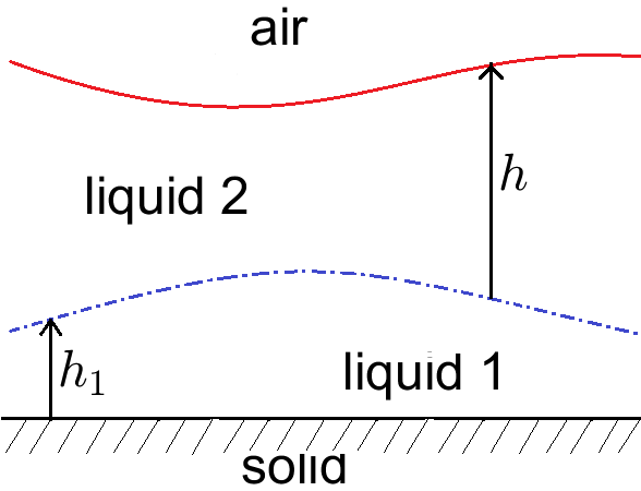
with and being the heights of the first and second liquid layers (cf. Fig.1), respectively, the ratio of the surface tensions (of the lower liquid layer
Figure 1: Sketch of two liquid layer height profiles and in (1).
over the upper one), and the intermolecular potential
(2)
with denoting a Lenard-Jones type potential
(3)
and parameter scaling the location of its minimum. In (3), and are the attractive and repulsive positive integer exponents, respectively, with . For the results of this article the concrete choice of is not important, the dependence on them will appear in the leading order formulae only through the absolute value of the potential minimum value (well’s depth):
For polymeric dewetting liquid films typically used choices of are or [16, 35, 3]. In numerical simulations of this article the latter choice is used.
with being the ratio of the liquid viscosities (of the lower layer over the upper one), which is set to in numerical simulations of system (1).
System (1) considered in interval with Neumann boundary conditions:
(4)
and initial conditions
(5)
has the unique positive classical smooth solution given sufficiently regular initial liquid height profiles and [19, 9].
Additionally, (1) equipped with (4) can be viewed as a gradient flow of the following energy functional [31, 32, 15]:
(6)
The masses of two liquids are conserved in this evolution, i.e.
(7a)
(7b)
with positive constants and (for simplicity both liquid densities are assumed to be equal to ). Positive stationary solutions to system (1)–(4) are critical points of the energy functional (6) and the corresponding Euler-Lagrange system can be written in the form:
(8a)
(8b)
(8c)
with constants and being the Lagrange multipliers (or constant hydrodynamic pressures of the first and second liquid layers) associated with conservation of masses (7a) and
(7b), respectively, and derivative of potential (3):
(9)
Additionally, we note that (8a)–(8b) can be rewritten as
From (9) and (11) we see that both and are positive if and for all . The latter conditions hold for most of the solutions to system (8a)–(8c) derived in this article.
Furthermore, multiplying (10a) and (10b) by and , respectively, and integrating them in by parts gives
Adding these two equalities yields
(12)
When expanded in powers of , (12) will provide us a relation between the leading orders of and for several solutions to system (8a)–(8c).
In this article, we address the following two questions about solutions to the dynamical system (1)-(4) and its stationary counterpart (8a)–(8c). Firstly, we are interested in understanding how the number and shape of solutions to (8a)–(8c) depends on the choice of physical and geometric parameters . For a sake of convenience, instead of masses from (7a)–(7b) we prefer to parameterize solution to (8a)–(8c) using parameters and related to and , respectively. A similar height parameter was effectively employed by asymptotic matching of the lens stationary solution in section 4.1 of [17]. Accordingly, in sections for broad ranges of positive (called below the model parameters) we derive the leading order formulae (in the asymptotic limit ) for the corresponding pressures and spatial profiles and of several non-constant solutions to system (8a)-(8b). Following [11, 20, 23, 17] our approach relies on systematic asymptotic matching of the repeated elementary solution blocks (bulk, contact line and ultra-thin film ones) described in section .
Correspondingly, we distinguish and describe eleven types of the so called composite solutions to (8a)–(8c) exhibiting from one up to four triple phase contact lines. Note that we do not address constant solutions to (1)-(4) or (8a)–(8c), having , and their connection to those found in sections by analyzing possible bifurcation paths. The latter analysis could be similar to the one done in [3, 32] and is out of the scope this article. Still as a preparation step for it, in section we plot and analyze the combined diagrams showing for broad ranges of the model parameters typical shapes of the existence domains (EDs) for all found non-constant solutions to (8a)–(8c) together.
Secondly, our numerical simulations of bilayer system (1)-(4) show that the eleven stationary solutions (found in sections ) are either dynamically stable or weakly translationally unstable when tested as initial conditions (5). By numerical solving of system (1)-(4) we extended and used the fully implicit finite differences scheme with adaptive time step developed in [30, 20, 24] for other coupled thin film models. Moreover, in section again using numerical simulations of system (1)-(4) we explain why all other composite stationary solutions to (1)-(4) are dynamically unstable and rather experience complex coarsening pathways (nevertheless converging in the long time to one of the stable states found in sections ). We conclude the article by discussing and comparing our results with the existing modeling and experimental ones and give an outlook in section 9.
2 Bulk, contact line and UTF profiles
Our aim is to construct different solutions to stationary system (8a)–(8c) by applying systematic asymptotic matching of the leading order expressions (as parameter in (3)) of typical bulk (B), contact line (CL) and ultra-thin film (UTF) profiles described in this section. For that, we assume formal (uniform in variable) asymptotic expansions
The bulk regions have length w.r.t and either or holds there. In CL regions, either or experiences a transition on a small interval of length around a point from the magnitude of to that one of UTF, i.e. to the leading order constant profile. Following the standard approach of [11, 12, 20, 23, 17] we use the change of variable
(14)
under which equations (8a)–(8b) in CL regions transform to equations
(15a)
(15b)
considered for .
Below we distinguish three bulk, four CL and one UTF types of regions and describe the corresponding leading order profiles of and in them.
Type I bulk profile:
both and are assumed to be functions as . Correspondingly, the leading order equations (8a)–(8b) take the form:
Integrating them twice in without applying boundary conditions the general type I bulk profiles are obtained:
(16)
In (16), and are four integration constants, the former giving the centers and the latter the maximum (or minimum) values of parabolic profiles and , respectively.
Type II bulk profile:
we assume and as , i.e. in asymptotic expansions (13) we set . To balance the potential terms in (8a)–(8b) we additionally set . Next,
using the following expansion of (9):
substituting into the first one, and integrating the latter twice in yields the general type II bulk profiles:
(18)
with and being two integration constants giving the center and the maximum values, respectively of concave parabolic profile .
Type III bulk profile:
we assume and as , i.e. in (13) one has and . Using again expansion (17) the leading order of (8a)–(8b) becomes
Expressing from the first equation
substituting into the second one, and integrating the latter twice in yields the general type III bulk profiles:
(19)
with and being the integration constants giving the center and the maximum values, respectively of concave parabolic profile .
UTF profile:
we assume and in (13). Using again (17), the leading order of (8a)–(8b) becomes
implying the second order constant profiles
Type I CL profile:
we assume and in (13), i.e. experiences a transition from to the leading order constant magnitude, while stays . Applying the variable change (14), the leading order of the scaled system (15a)–(15b) becomes
(20a)
(20b)
with potential from (3). In turn, the first order corrector equation for (15b) takes the form . Next, integrating (20a) once and (20b) twice in one obtains
(21a)
(21b)
with being the integration constants. The sign of in (21a) is positive (negative)
if is increasing (decreasing).
Type II CL profile:
we assume and in (13), i.e. experiences a transition from to the leading order constant magnitude, while stays . Applying again (14), the leading order of (15a)–(15b) becomes
(22a)
(22b)
In turn, the first order corrector equation for (15a) takes the form:
Next, integrating once (22b) and (22a) twice in one obtains
(23a)
(23b)
with being the integration constants.
Type III CL profile:
we assume in (13) with experiencing a transition from to the leading order constant magnitude, while . Applying (14) the leading order of (15a)–(15b) becomes
This system can be rewritten as
(24a)
(24b)
Multiplying (24a) and (24b) by and , respectively, and integrating them for by parts gives
where we used and . These imply together
and, consequently, switching back to variable in (14), the macroscopic contact angle:
(25)
is obtained. In the last step, we used .
Type IV CL profile:
we assume in (13) with experiencing a transition from to the leading order constant magnitude, while . Applying (14), the leading order of (15a)–(15b) can be again written in the form (24a)–(24b). Integrating it for leads now to
where we used and . These imply together
and, consequently, the macroscopic contact angle:
(26)
3One-CL solutions
In this section, we classify and derive the leading order profiles of the solutions to system (8a)–(8c) having one contact line. Up to a possible inversion of -variable we distinguish four types of such solutions: lens, internal drop, -drop, and -drop ones.
Lens: The solution is obtained by matching Type I (with ) and Type II (with ) bulk solutions to Type II CL ones centered around . For that we rewrite the bulk solutions (16) and (18) as functions of the inner CL variable using (14), expand them in powers of , and subsequently match the leading orders of them and their first derivatives (w.r.t. ) to the corresponding expansions of CL solutions (23a)–(23b). This procedure leads to the following set of matching conditions:
(27)
Additionally, we fix and as the given maximum values of and , respectively. System (27) has equations with unknowns: and . From its last two equations we find . Substituting that into the equation in (27) gives . Dividing the over the last equations in (27) provides expressions
The derived lens solution is well defined if the following two constraints are obeyed:
(28)
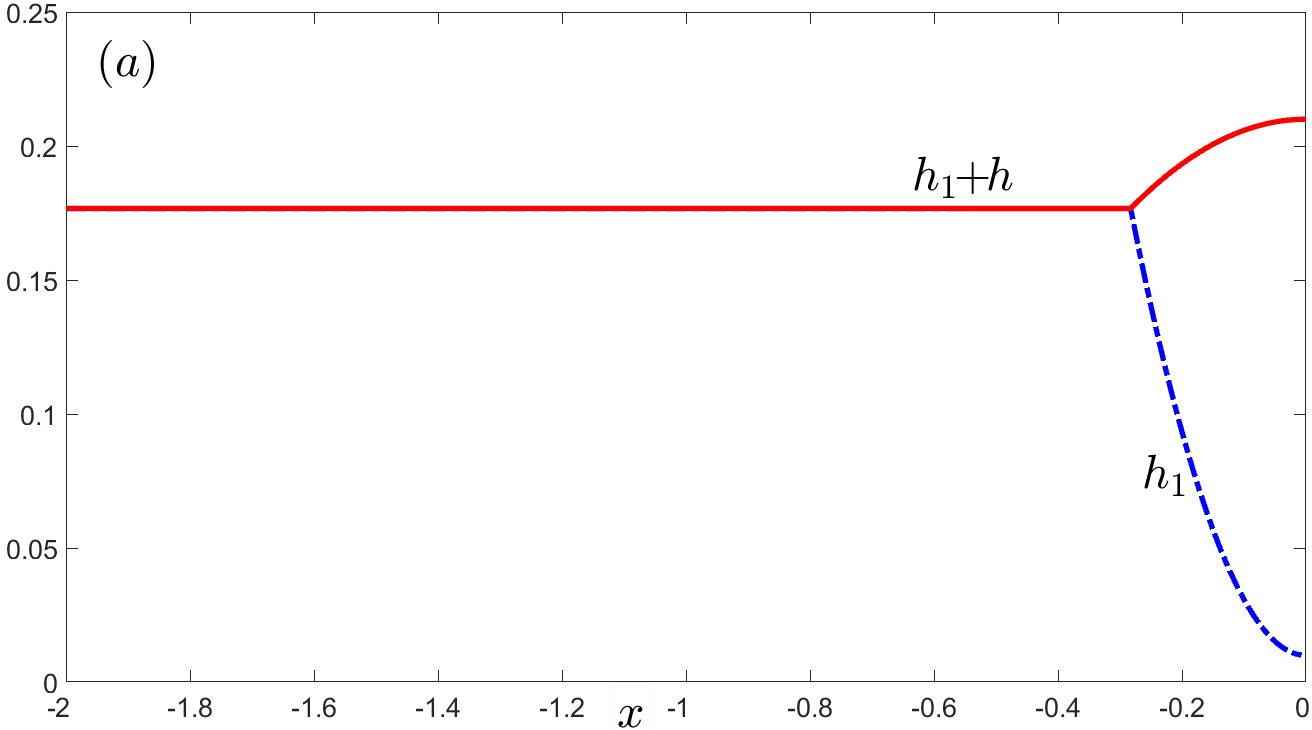
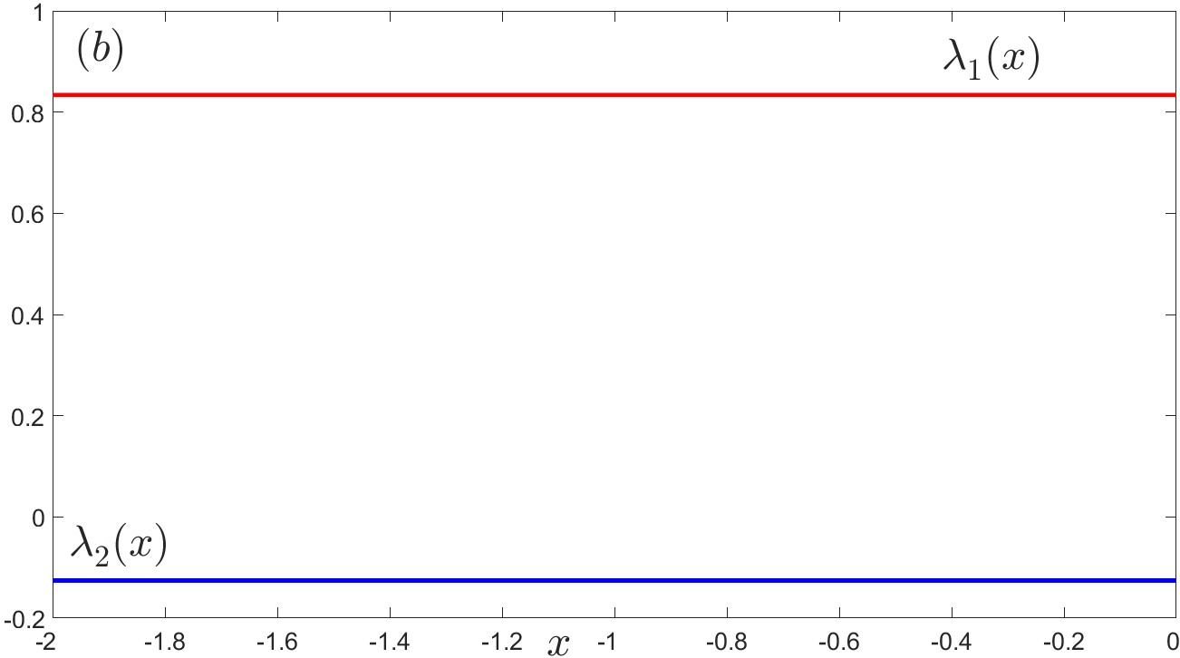
Note that the second constraint sets a relation between the maximal heights for which both and stay positive for all , while the first one controls the minimal interval length in which the solution can be allocated. Typical shape of the lens solution is shown in Fig.2 (a).
Internal drop: The solution is obtained by matching Type I (with ) and Type III (with ) bulk solutions to Type I CL ones centered around . Again we use (14) and match (16), (19) and their first derivatives (w.r.t. ) to the corresponding expansions of (21a)–(21b). This procedure leads to the following set of matching conditions:
(29)
Additionally, we fix and . System (29) has equations with unknowns: and . Solving it proceeds similar to that one of system (27) for the lens solution and yields the expressions
Figure 2: Numerical lens stationary solution (a) to system (1)–(4) for , with constant pressures (b) .
as well as two constraints:
(30)
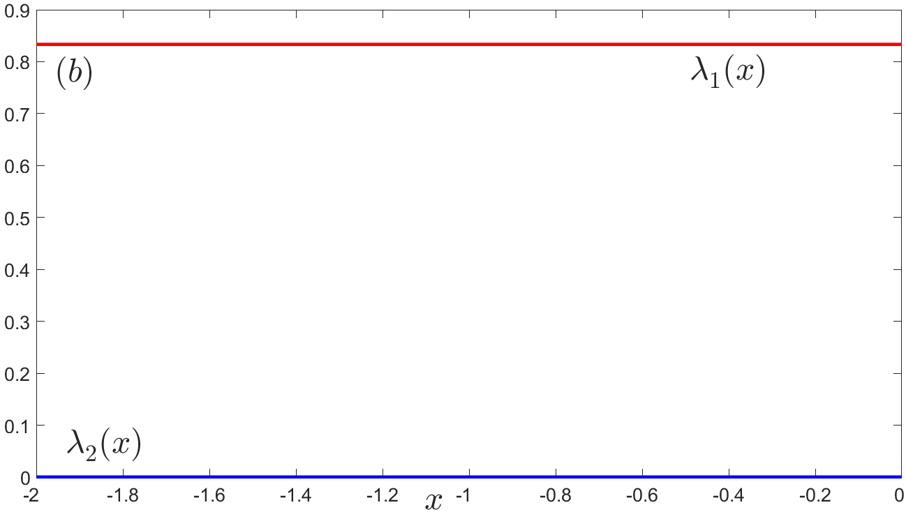
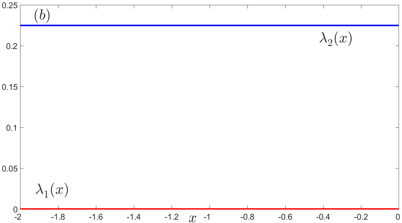
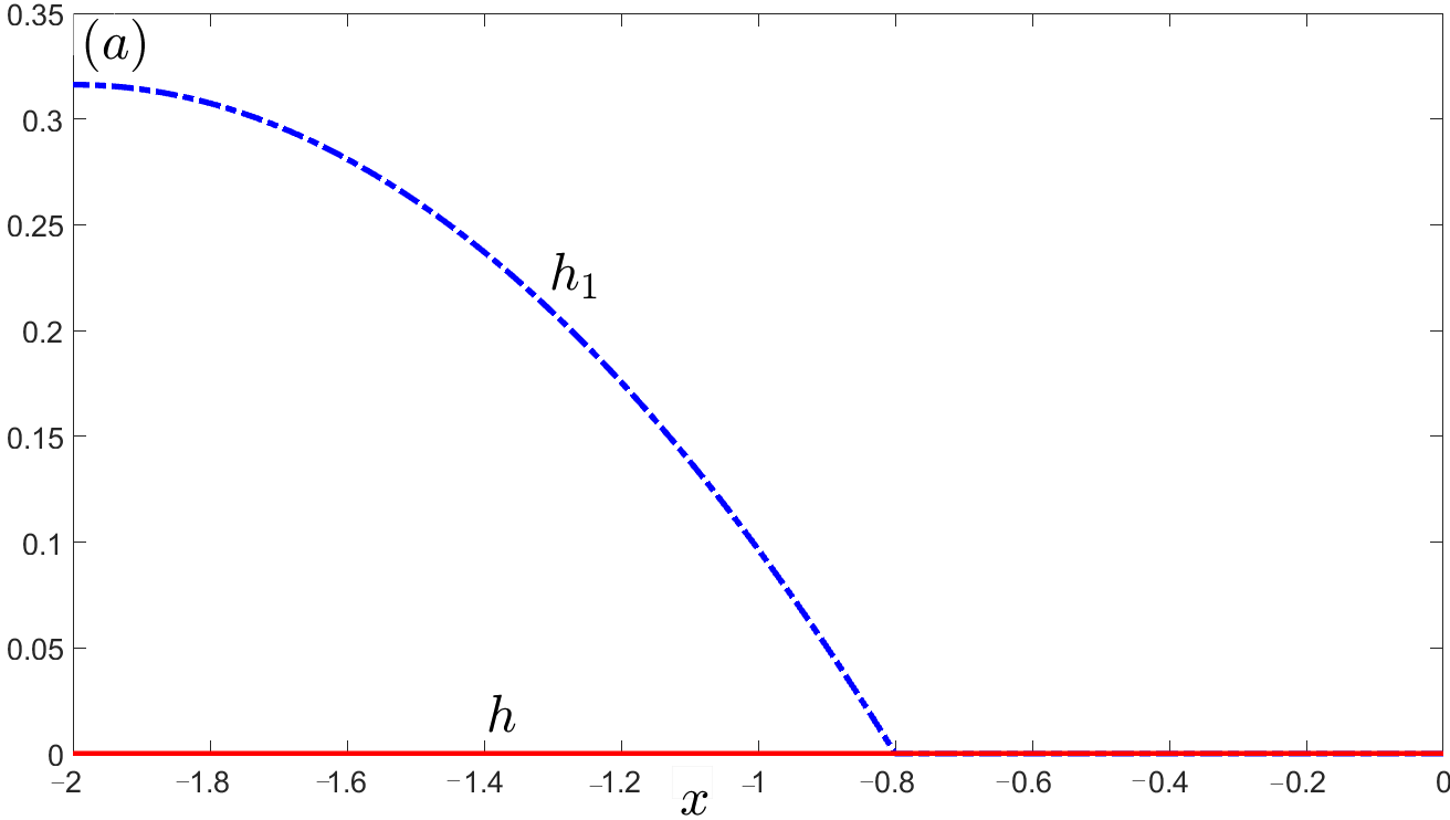
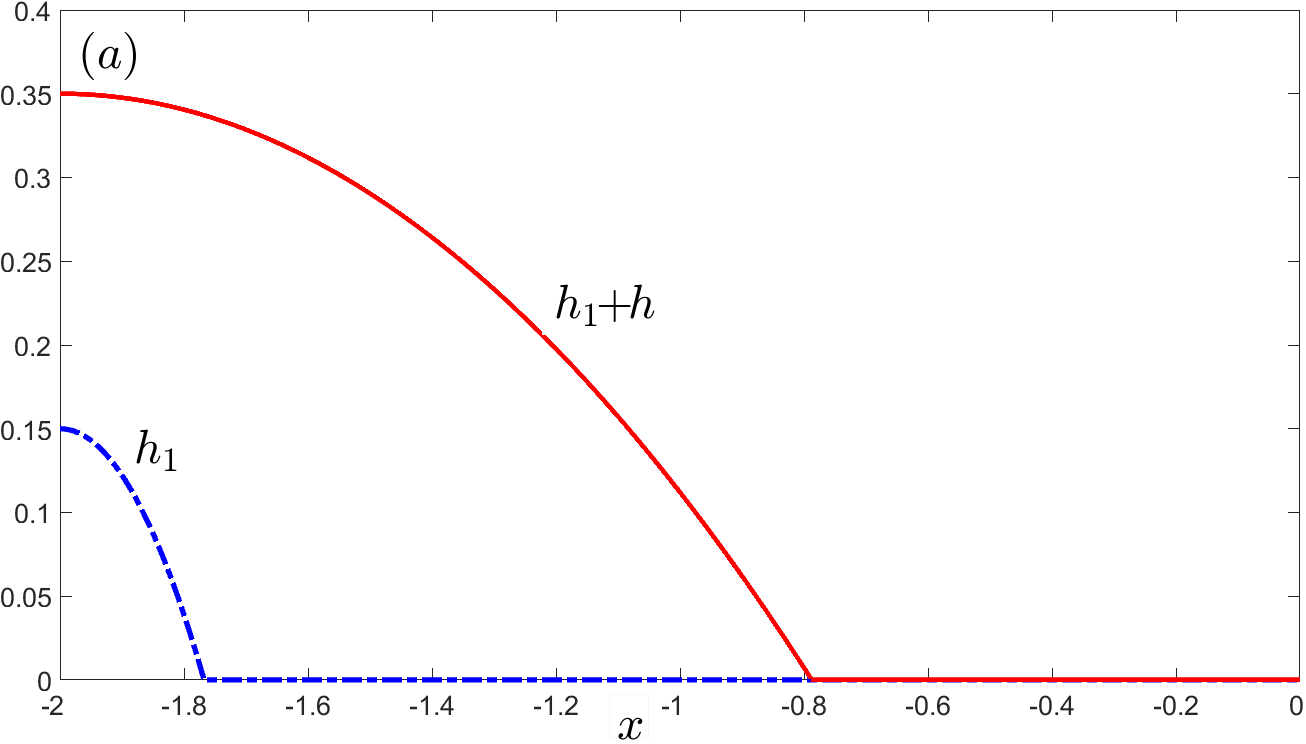
Additionally, we note that holds for all , i.e. the second fluid layer is uniformly flat, while the first one has the form of a parabolic drop. Typical shape of the internal drop solution is shown in Fig.3 (a).
Figure 3: Numerical internal drop stationary solution (a) to system (1)–(4) for with constant pressures (b) .
-drop: The solution is obtained by matching Type II (with ) bulk and UTF solutions to Type III CL ones centered around . We match (18) using contact angle condition (25) to get
(31)
implying that
The only constraint imposed on this solution is , i.e. the one controlling the minimal length :
(32)
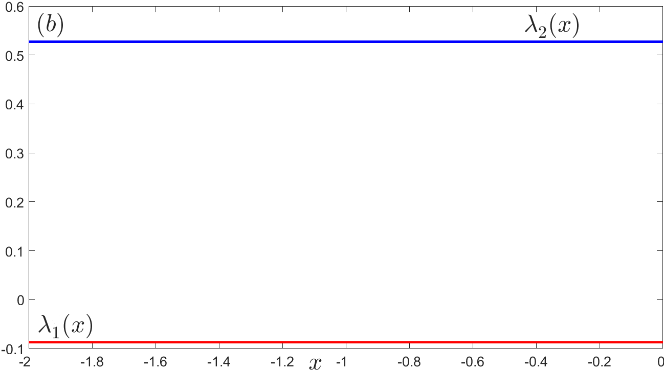
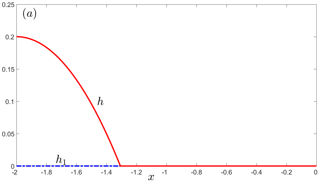
Note, that system (31) does not determine the value of , which is observed to be nonzero and negative in the numerically found -drop solutions, a typical shape of which is shown in Fig.4 (a).
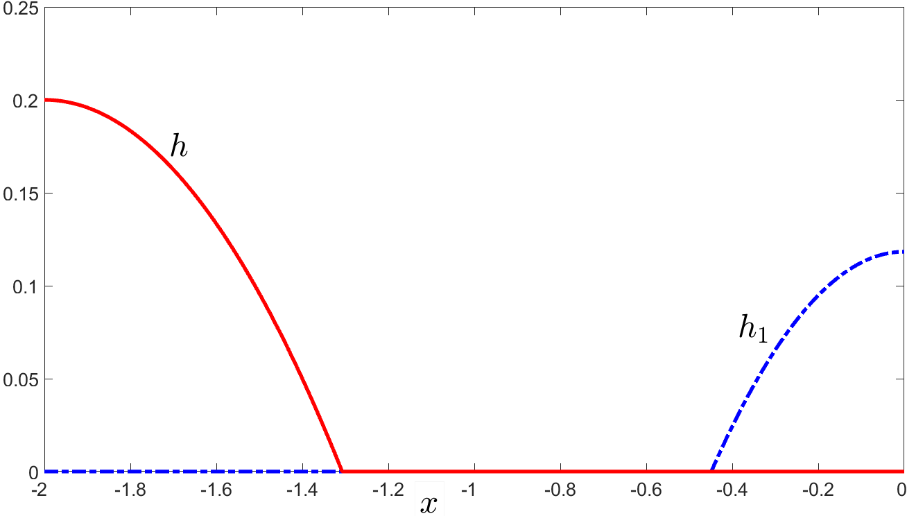
Figure 4: Numerical -drop stationary solution (a) to system (1)–(4) for with constant pressures (b) , .
-drop: The solution is obtained by matching Type III (with ) bulk and UTF solutions to Type IV CL ones centered around . We match (19) using contact angle condition (26) to get
(33)
implying that
Figure 5: Numerical -drop stationary solution (a) to system (1)–(4) for with constant pressures (b) , .
The only constraint imposed on this solution is again , i.e.
(34)
Again system (33) does not determine the value of , which is observed to be nonzero and negative in the numerically found -drop solutions, a typical shape of which is shown in Fig.5 (a).
4Two-CL solutions
In this section, we classify and derive the leading order profiles of the solutions to system (8a)–(8c) having two contact lines. Up to a possible inversion of -variable we distinguish four types of them: zig-zag, sessile lens, sessile internal drop, and -drops ones.
Zig-zag: The solution is obtained from the combined matching of general Type I and Type III (with ) bulk solutions to Type I CL ones centered around ( CL) as well as of general Type I and Type II (with ) bulk solutions to Type II CL ones centered around ( CL). Schematically this matching chain can be encrypted as once moving in from to .
At the contact line points and we apply analogous procedures to those used in section 3 for the one-CL solutions involving the matching of them and their first derivatives. For shortness, we omit the details and just state the resulting system of the leading order matching conditions:
(35)
Additionally, we fix and . System (35) has equations with unknowns: and .
From the linear part of this system, i.e. by performing joint manipulations with the 2nd, 5-6th, 9-10th, and 12th equations in (35), the following expressions for positions are obtained:
(36)
In turn, the rest of the equations of system (35) imply two quadratic relations
(37a)
(37b)
from which the expressions for and in terms of the model parameters
can be derived as follows.
First, we substitute expressions (36) into (37a) and divide both sides of the latter by to get
Next, expanding the squares on both sides of this equality and, subsequently, multiplying it by yields after few term cancellations
(38)
Similarly, substituting (36) into (37b) one derives another relation
Adding the last two relations gives
implying that
(39)
Finally, dividing (38) by and using (39) yields a quadratic equation for :
having single positive root:
(40)
Note that taking , instead, would imply by (39) and, subsequently, contradict to conditions (this can be checked using explicit expressions (36)).
In summary, formulae (36), (39) and (40) provide a complete information about the leading order (as ) profile of the derived zig-zag solution with typical shapes of which being shown in Fig.6.
They also cover the two limiting cases and in system (35), which correspond to
or values in (39), respectively. In these cases, profile of or , in the bulk region is given by a linear segment and
The corresponding limiting formulae for positions can be derived from (36) then.
The constraints on the zig-zag solution are deduced from the length ones
(41)
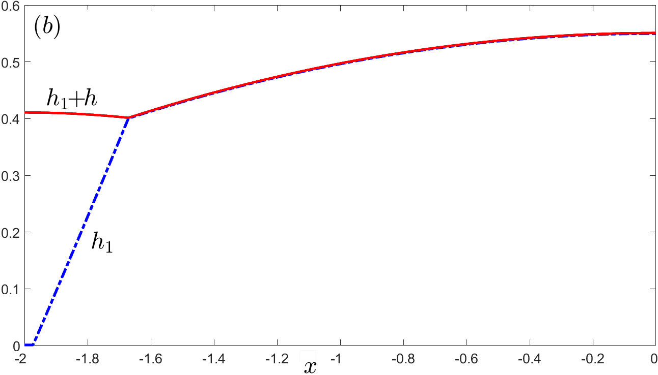
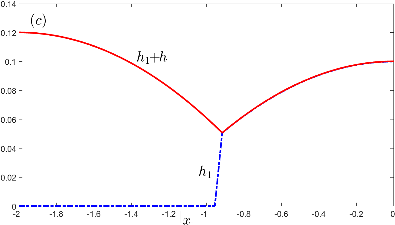
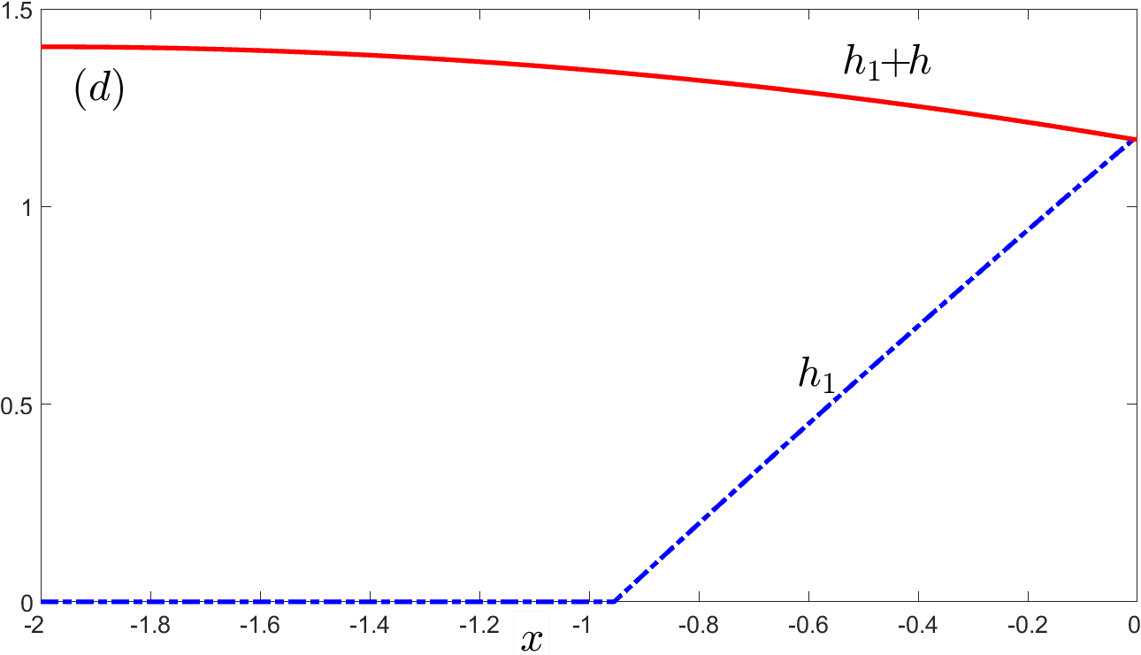
Figure 6: Numerical zig-zag stationary solutions to system (1)–(4) for , with observed: (a) ; (b) ; (c) ; (d) .
as follows. First, note that from the , 6th and 10th equation of system (35) it follows that is monotonically decreasing function. Similarly, from the 12th, 9th and 5th equations in (35) it follows that is monotonically increasing. Therefore, if the length conditions (41) are assured then the leading order profile of zig-zag solution described above is well defined.
For instance, let . Using formulae (36) conditions (41) can be written then as
As , these inequalities reduce to constraint
(42)
Next, substituting the expression (40) for in (42) and using allow us to deduce
(43)
Finally, using decomposition
simplifies (43) further and implies the following bounds on the interval length from above and below:
Similar constraints on can be deduced using formulae (36) and (40) for the other two ranges and . We omit the details and just state their combined final form being valid for all positive :
(44)
Constraints (44) cover also the two limiting cases and occurring for and values, respectively. Note that the interval boundaries , and in (44) correspond to the critical merges , and , respectively, occurring when one of the bulk regions in zig-zag solution shrinks to zero (cf. Fig.6 (b)-(d)). Accordingly, special value in (44) sets a threshold between the cases when either or merge occurs first by decreasing . Additionally, note that merge occurs simultaneously with and , i.e. the solution splits into a 2-drops one (described below in this section) then (cf. Fig.6 (c)).
Sessile lens: The solution is obtained by a combined matching of Type I (with ) and general Type II bulk solutions to Type II CL ones centered around ( CL) as well as of general Type II bulk and UTF solutions to Type III CL ones centered around ( CL). Schematically this matching chain can be encrypted as once moving in from to .
After the matching procedures at contact line points and the resulting system of the leading order conditions takes the form:
(45)
Additionally, we fix and . System (45) has equations with unknowns: and . From the linear part of system (45), i.e. by performing joint manipulations with its and 6th equations, one deduces that . Next, from the last two equations in (45) one obtains . Substituting that into the equation in (45) and, subsequently, subtracting from it the and equations yields a relation
(46)
Next, from the and equations in (45) one deduces a relation
Finally, substituting (46)–(48) into the and equations in (45) yields the expressions for the contact line positions:
(49)
In summary, formulae and (46)–(49) provide a complete information about the derived sessile lens solution, typical shapes of which are shown in Fig.7.
In particular, from the equation in (45) one gets
(50)
implying the following combined formula for the maximum value of :
(51)
Additionally, for (46) and (48) imply the presence of critical case for which and holds for all , i.e. the leading order profile of in the left bulk region is flat (cf. Fig.7 (c)). From (47) we observe that the second critical case is not possible here.
The constraints on the sessile lens solution are deduced again from conditions (41)
using (49) and take the form:
(52)
The first condition in (52) provides the bound on the minimal interval length , while the second one ensures and is required only if . The threshold
corresponds to the contact line merge occurring simultaneously with (cf. (50)–(51) and Fig.7 (d)).
Sessile internal drop: The solution is obtained by a combined matching of Type I (with ) and general Type III bulk solutions to Type I CL ones centered around ( CL) as well as of general Type III bulk and UTF solutions to Type IV CL ones centered around ( CL).
Figure 7: Numerical sessile lens stationary solution to system (1)–(4) for : (a) and ; (b) and ; (c) and , ; (d) and .
The matching chain can be encrypted as once moving in from to .
After the matching procedures at contact lines and the resulting system of the leading order conditions takes the form:
(53)
Additionally, we fix and . System (53) has equations with unknowns: and . Its solution proceeds
similarly to the one of system (45) for the sessile lens solution. From the linear part of system (53) one deduces that . Next, from the last two equations in (45) one obtains . Substituting that into the equation in (45) and, subsequently, subtracting from it the and equations one arrives at relation
Finally, substituting (54)–(55) into the and equations in (53) yields:
(56)
Figure 8: Numerical sessile internal drop stationary solution to system (1)–(4) for : (a) and ; (b) and .
In summary, formulae and (54)–(56) provide a complete information about the derived sessile internal drop solution, typical shapes of which are shown in Fig.8. In particular, expressions (54)–(55) imply for the presence of critical case for which and holds for all , i.e. the leading order profile of in the left bulk region is flat. Accordingly, one has
(57)
From (55) we note that the second critical case is not possible here.
The constraints on the sessile internal drop are deduced again from conditions (41)
using (56) and take the form:
(58)
The second condition in (58) ensures and is required only if . The threshold
corresponds to the contact line merge with (cf. Fig.8 (b)).
2-drops: The solution is obtained from simple concatenation of -drop and -drop solutions. The matching chain can be encrypted as – once moving in from to . The corresponding system of matching conditions is simply the union of (31) and (33) ones with the former ones being shifted to instead of and, subsequently, reflected around the origin, while in the latter ones replaced by . The resulting system of four equations implies the following expressions:
A typical shape of 2-drops solution is shown in Fig.9. The only constraint imposed on it is
(59)
Figure 9: Numerical 2-drops stationary solution to system (1)–(4) for with .
5Four-CL solutions
For certain symmetry reasons we classify and describe the three contact line solutions in the next section. Before that in this section, we derive the leading order profiles of the solutions to system (8a)–(8c) having four contact lines.
Up to possible inversion of -variable we find a single solution type denoted below as 2-side sessile zig-zag.
2-side sessile zig-zag: The solution is obtained by a combined matching of the following leading order profiles: UTF and general Type II bulk solutions to Type III CL centered around ( CL); general Type I and Type II bulk to Type II CL ones centered around ( CL); general Type I and Type III bulk solutions to Type I CL ones centered around ( CL); as well as UTF and general Type III bulk solutions to Type IV CL centered around ( CL). Schematically this matching chain can be encrypted as – once moving in from to .
At the four contact line points we apply analogous procedures to those used in sections 3-4 involving matching of the solutions and of their first derivatives. We omit the details and just state the resulting system of the matching conditions:
(60)
Additionally, we fix and . System (60) has equations with unknowns: and . In fact, due to a translation invariance (within interval ) possessed by this solution one of the four parameters can be chosen as a free (shift) parameter, which makes (60) an overdetermined algebraic system.
From the first and the last two equations in (60) one easily obtains expressions
(61)
Similarly, dividing the over the equation in (60) and using (61) yields
(62)
while dividing the over the equation in (60) gives .
In turn, dividing the over the equation in (60) and using the last two expressions yields
(63)
Comparing expressions (62)–(63) one deduces a quadratic equation for :
(64)
Further, substituting (61) into (64) yields a unique positive solution to the latter:
(65)
Proceeding similarly, after deducing expression
from the and equations in (60) and manipulating with ones yields relations
(66a)
(66b)
Next, substituting (61) into (66b) one finds a unique positive solution to the latter:
(67)
Finally, letting be a free (shift) parameter from the linear part of system (60), i.e. by manipulating with the , , , , , and equations in (60), the following expressions for the positions are obtained inductively:
(68)
Note that two different expressions for in (68) are consistent with each other. They can be rewritten as
One can show validity of the last relation using expressions (63)–(64) and (66a)–(66b) arguing similarly as in the next following argument that crosschecks satisfaction of the quadratic equations in system (60).
By manipulating with the 3rd, 5th, and 9th equations in (60) one deduces a combined quadratic relation
Next, multiplying both sides by along with bracket opening yields
Finally, substituting expression (63) for and subsequently using (64) reduces the last relation simply to the expression of in (61).
Similarly, using (66a)–(66b) and (68) one verifies another combined quadratic relation
(70)
which is deduced from the 13rd, 10th, and 6th equations in (60).
In summary, formulae (61), (63), (65), (66a) and (67)–(68) provide a complete information about the leading order (as ) profile of the derived 2-side sessile zig-zag solution, typical shapes of which are shown in Fig.10. They also cover the two limiting cases and in system (60) corresponding to
Figure 10: Numerical 2-side sessile zig-zag solution to system (1)–(4) for : (a) ; (b) , ; (c) , (-variable inverted); (d) numerically observed pressure profile for solution in (b).
or values, respectively, in (65) and (67). In these cases, profile of or in the bulk region is given by a linear segment. The corresponding limiting formulae for positions can be derived then from (68).
Note that in contrast to stationary solutions to system (1)–(4) of sections , 2-side sessile zig-zag is not dynamically stable one. In particular, that is indicated
by the spikes observed in the pressures profile of Fig.10 (d) around and contact lines. Nevertheless, numerical simulations of system (1)-(4) show that solutions of Fig.10 (a)–(c) translate extremely slow to one of the interval ends or without changing their leading order shape. Such behavior was already observed for symmetric drop solutions in one-layer lubrication equations [3] with their translational instability originating from a single exponentially small eigenvalue in the spectra [22] of the corresponding linearized operators. Therefore, 2-side sessile zig-zag is a weakly unstable stationary solution to system (1)–(4).
The constraints on 2-side sessile zig-zag are deduced from the length ones
(71)
as follows. From the expressions for and in (68) it follows that the constraint is satisfied if
If , i.e. when , the last inequality reduces to
(72)
Substituting (66a) and subsequently expressions (67) and (61) into (72) gives
which indeed holds if . In turn, if , the inequality in (72) is reversed and its satisfaction for follows by a similar argument. Therefore, we conclude that holds for all positive .
Next, using expressions in (68) the constraints and can be rewritten as
respectively. Analogously, one shows that these two inequalities hold for all using relations (66a) or (63) with subsequent substitution of expressions (67) or (65), respectively, along with (61).
Finally, the first and the last inequalities in (71) result in the constraints on the minimal interval length and the maximal free shift parameter , respectively. Namely, the two conditions imposed on 2-side sessile zig-zag can be written as
(73)
Additionally, we note that the maxima of and in are given by values and , respectively, only when and hold.
Using expressions (68) and (63), (66a) one checks that the latter two conditions are equivalent to
and ones, respectively, which in turn by (61) reduce to and (as before ).
Therefore, the following combined formula holds
In order to invert formula (74), i.e. to find out how values and depend on the given maxima of and let us denote
(75)
In the case , inverting formula (67) using (74) yields:
Analyzing the last inequality one observes that only sign is possible there leading, subsequently, to condition . Arguing similarly for the case by inverting now formula (65) one obtains an equivalent condition . Combining all together yields the following inverse formula to (74):
(76)
6Three-CL solutions
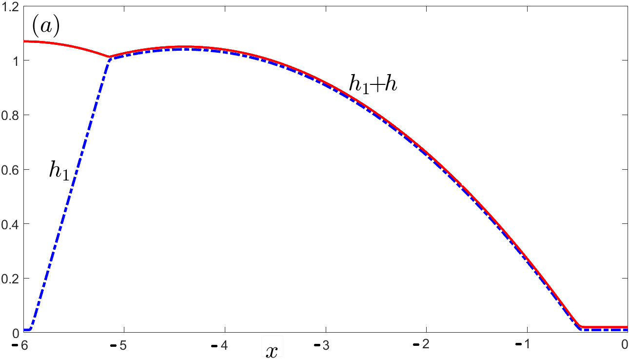
In this section, we classify and derive the leading order profiles of the solutions to system (8a)–(8c) having three contact lines. Up to a possible inversion of -variable we find two solution types denoted below as -sessile zig-zag and -sessile zig-zag. Due to the fact that both solution types can be viewed as opposite parts of the 2-side sessile zig-zag described in section 5 derivation of their leading order profiles proceeds analogously.
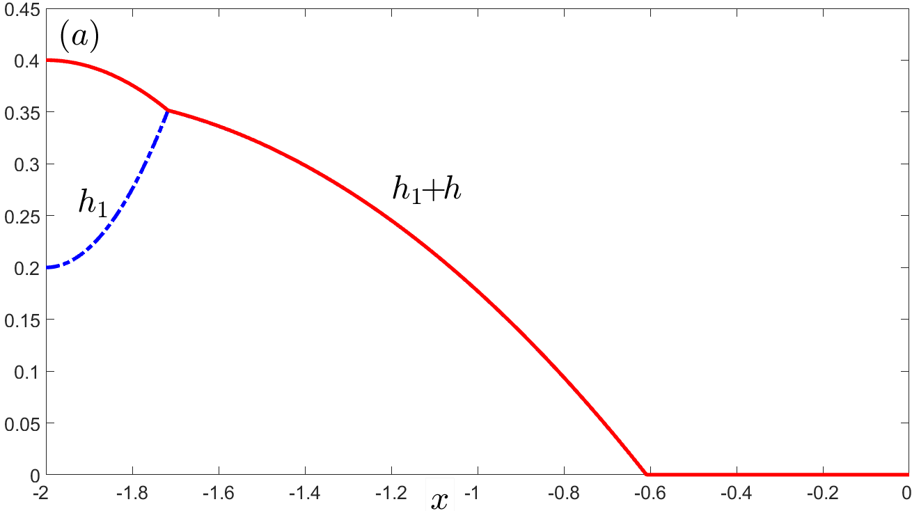
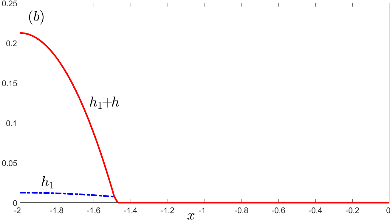
-sessile zig-zag: The solution is obtained by a combined matching of the following leading order profiles: general Type I and Type II bulk (with ) solutions to Type II CL ones centered around ( CL); general Type I and Type III bulk solutions to Type I CL ones centered around ( CL); as well as UTF and general Type III bulk solutions to Type IV CL centered around ( CL). Schematically this matching chain can be encrypted as – once moving in from to .
Applying the matching procedure at the three contact points one obtains the following system:
(77)
Additionally, we fix and . System (77) has equations with unknowns: and .
Next, relation (12) expanded for the considered solution in powers of yields after retaining only the leading order terms:
(79)
The rest of solving system (77) proceeds exactly as for (60) in section 5. Namely, from the , , , and equations in (77) we derive expressions (63)-(65), while from the , , , and ones (66a)–(67). In turn, from the linear part of system (77) the following expressions for the positions are obtained inductively:
(80)
Note that consistency of two different expressions for in (80) as well as validity crosschecks for the quadratic relations in (77) can be verified using (63)–(64) and (66a)–(66b) analogously as was done in section 5 for system (60).
In summary, formulae (78)–(79), (63), (65), (66a), (67), and (80) provide a complete information about the leading order (as ) profile of the derived -sessile zig-zag solution, typical shapes of which are shown in Fig.11. They also cover one limiting case in system (77), which correspond to value in (65) and (67). In this case, profile of in the bulk region is given by a linear segment. The corresponding limiting formulae for positions can be derived then from (80). The limiting case is not possible for solutions of (77), as shown in the next paragraph it corresponds to the merge .
The constraints on the solution are deduced from the length ones
(81)
as follows. Arguing similar as for (71) in section 5 one shows that conditions and hold automatically for all . Next, using (80) condition transforms to and, subsequently, by (63) to , i.e. using (78)–(79) to the constraint (cf. Fig.11 (a)). Finally, using (80) together with (66a) one shows that condition imposes the following bound:
Figure 11: Numerical -sessile zig-zag stationary solution to system (1)–(4) for : (a) and ; (b) and .
(82)
Additionally, note that only when . Using (80), (66a) one checks that the latter condition is equivalent to which, in turn, by (61) reduces to . Therefore, the combined formula
(83)
holds with given by (67). Further, setting as in (75) and proceeding analogously to the derivation of (76) in section 5, i.e. by
inverting formula (67) for , one obtains the inverse formula to (83):
(84)
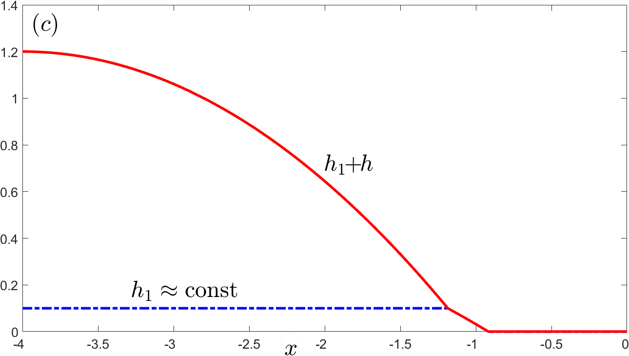
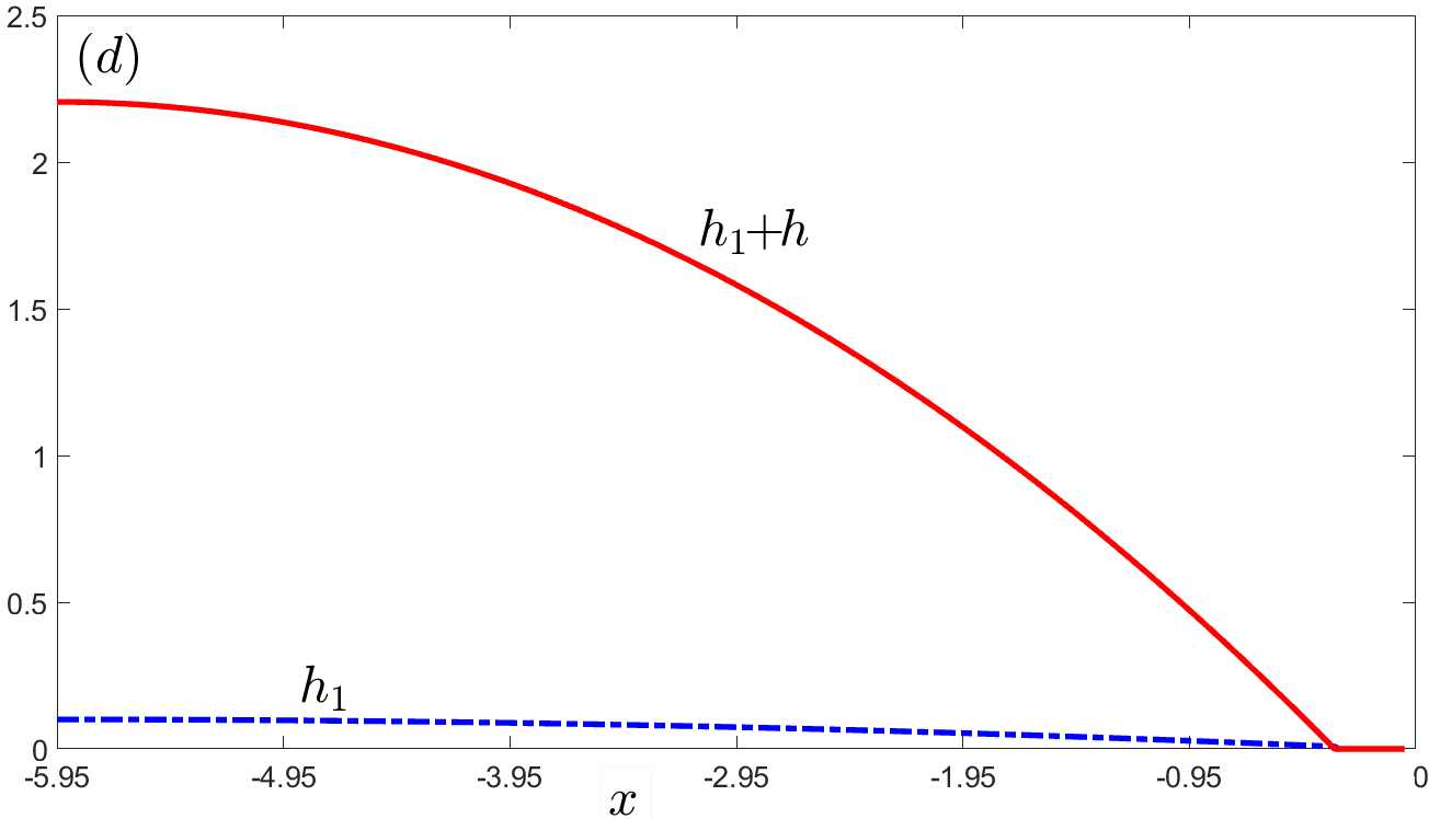
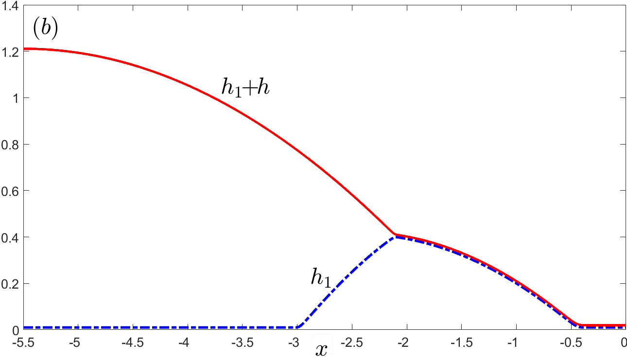
-sessile zig-zag: The matching chain for this solution can be encrypted as if moving in from to .
Applying the matching procedure at the three contact points yields:
(85)
Figure 12: Numerical -sessile zig-zag stationary solution to system (1)–(4) for : (a) and ; (b) and .
Additionally, we fix and . System (85) has equations with unknowns: and .
Solution procedure for system (85) is very similar to the ones for (77) and (60) described before. Therefore, we omit the details and state just the solutions formulae. Again all expressions (61)–(67) remain true with a small exception that signs of (63) and (66a) are reversed, because -sessile zig-zag can be viewed as the right part of the 2-side sessile zig-zag solution (cf. Fig.10 and Fig.12). In turn, the positions expressions take the form:
(86)
Typical shapes of -sessile zig-zag solutions are shown in Fig.12.
The constraints on -sessile zig-zag solution are deduced from (81). Again, conditions and hold for all , while reduces now to condition (cf. Fig.12 (a)). In turn, condition impose a bound on the minimal interval length :
(87)
Additionally, the combined formula for the maximum of takes the form
(88)
with given by (65), while inverting the latter formula for yields:
In sections 3-6, we described 11 types of stationary solutions to bilayer system (1)–(4) together with the leading order explicit conditions on the model parameters for which
such solutions exist and are well defined for all sufficiently small . In this section, using the latter conditions we plot and discuss the combined diagrams showing for broad ranges
of the model parameters typical shapes of the existence domains (EDs) for all found solutions together.
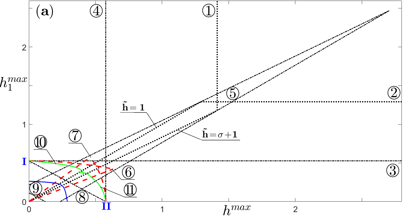
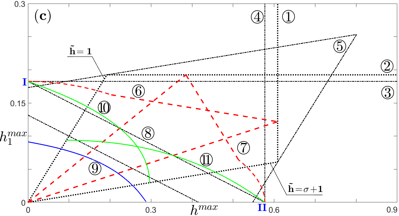
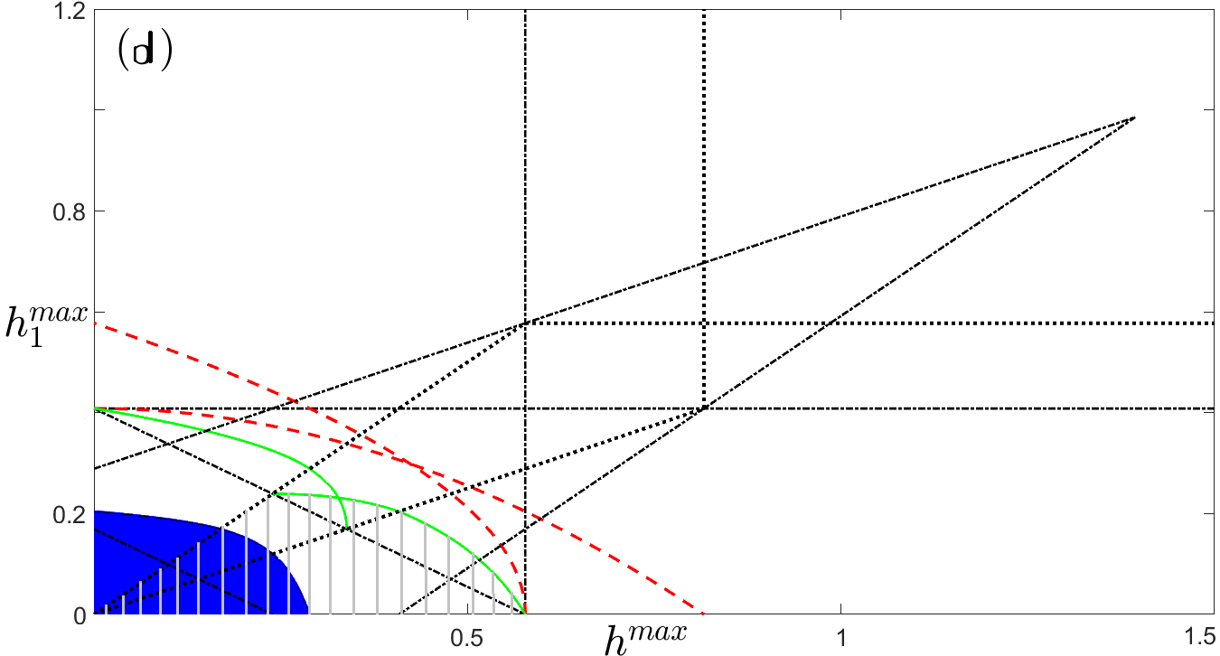
In Fig.13, we fix parameters and and plot for three different values of the solution diagrams w.r.t. two variables
with their ratio denoted below by similarly as in (75). The domain boundaries for different solutions are indicated in Fig.13 by numbers as follows:
\raisebox{-.9pt} {1}⃝–lens, \raisebox{-.9pt} {2}⃝–internal drop, \raisebox{-1.1pt} {3}⃝–-drop,
\raisebox{-.9pt} {4}⃝–-drop, \raisebox{-1.pt} {5}⃝–zig-zag, \raisebox{-.9pt} {6}⃝–sessile lens,
\raisebox{-1.pt} {7}⃝–sessile internal drop, \raisebox{-1.pt} {8}⃝--drops, \raisebox{-.9pt} {9}⃝–2-side sessile zig-zag, \hspace{-.05cm}\raisebox{-1.1pt} {1\!0}⃝–-sessile zig-zag, \raisebox{-1.pt} {1\!1}⃝–-sessile zig-zag.
From their explicit formulae we observe that all EDs are open and simply connected and their boundaries in many cases, except only for solutions \raisebox{-.9pt} {6}⃝–\raisebox{-1.pt} {7}⃝
and \raisebox{-.9pt} {9}⃝–\raisebox{-1.pt} {1\!1}⃝, are formed by intersecting straight lines. For example, EDs of lens \raisebox{-1.1pt} {1}⃝ or internal drop \raisebox{-.9pt} {2}⃝ solutions are semi-infinite stripes bounded by or lines, respectively, and another vertical or horizontal ones (cf. (28) and (30)); -drops \raisebox{-1.pt} {8}⃝ ED is given by a right triangle with its hypotenuse connecting the base points of the horizontal and vertical lines forming the ED boundaries for -drop \raisebox{-1.1pt} {3}⃝ and -drop \raisebox{-.9pt} {4}⃝ solutions, respectively (cf. (59) and (32)–(34)); zig-zag solution \raisebox{-1.pt} {5}⃝ lives in a pentagon domain formed by the intersection of the coordinate axes and three lines (cf. (44)):
(90a)
(90b)
For sessile lens\raisebox{-.9pt} {6}⃝ the curvelinear shape of its ED boundary qualitatively differs in two cases when or (cf. (51)–(52)).
For the ED is confined to a sector bounded by parabola
The latter boundary line corresponds to singular merge (cf. Fig.7 (a)) and coincides with axis when .
For the ED is a sector bounded by the same parabola and two other lines:
with the latter one corresponding to the singular merge shown in Fig.7 (d).
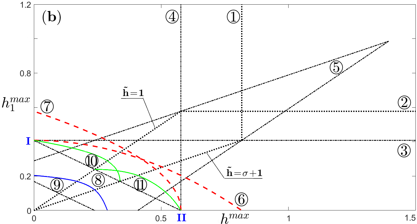
Figure 13: Combined diagrams showing existence domains (EDs) for 11 solution types found in this article for and (a) ; (b) and (d) ; (c) .
ED boundaries are shown for the solutions as dotted, and as dash–dotted, as dashed, as solid curves. In (d), EDs of and solutions are filled with solid and dashed colors, respectively. Symmetric points and are located at and , respectively.
Similarly, for sessile internal drop\raisebox{-1.pt} {7}⃝ the shape of its ED depends on the case or (cf. (57)–(58)).
For the ED is a sector bounded by parabola
coinciding with axis when . For the ED sector is bounded by the same parabola and two other lines:
with the latter one corresponding to the singular merge shown in Fig.8 (b).
For 2-side sessile zig-zag\raisebox{-.9pt} {9}⃝ ED is a sector (cf. Fig.13 (d)) formed by the intersection of the coordinated axes and
and the curve
This formula follows from the constraints (73) after substituting into them expressions (68) where explicit formulae (61), (65), (67) and (63), (66a) are used with as before . By plotting this curve in Fig.13 we employed the transformation relations (74), (76) between and .
For -sessile zig-zag\hspace{-.05cm}\raisebox{-1.1pt} {1\!0}⃝ ED is a sector formed by the intersection of line
and the curve
This formula follows from the constraint (82) using (61) and (67). By plotting this curve in Fig.13 we employed the transformation relations (83)–(84) between and . Similarly, for -sessile zig-zag\raisebox{-1.pt} {1\!1}⃝ ED is a sector (cf. Fig.13 (d)) formed by the intersection of line and the curve
This formula follows from the constraint (87) using (61) and (65). By plotting this curve in Fig.13 we employed the transformation relations (88)–(89) between and .
In summary, the EDs boundaries of the solutions to system (1)–(4) and its stationary counterpart (8a)–(8c) derived in sections 3-6 depend linearly on the product and, therefore, their form is simply rescaled under changes of parameters or , while qualitatively differs only in three cases , or demonstrated in Fig.13. Interestingly, all presented solution diagrams are symmetric around the special line connecting the origin with the acute peak of the ED boundary of zig-zag\raisebox{-1.pt} {5}⃝. More precisely, the solution diagrams do not change if they are reflected around line in the transversal direction of one. Note that the latter is the direction of the ED boundary of -drops solution \raisebox{-1.pt} {8}⃝ as well as of the first line in (90a). In special case , the solution diagram possesses additional symmetries (see Fig.13 (b), (d)). For example, the ED boundaries for solutions \raisebox{-.9pt} {2}⃝, \raisebox{-1.pt} {8}⃝ and \raisebox{-1.pt} {1\!1}⃝ intersect at a single joint point, while those for \raisebox{-.9pt} {2}⃝, \raisebox{-.9pt} {4}⃝ and \raisebox{-1.pt} {5}⃝ at another one.
Additionally, Fig.13 reveals special symmetric points depicted there as and at which two quadruples of ED boundaries originate together with three out of four in them tangentially to each other. At point , these are ED boundaries for \raisebox{-1.1pt} {3}⃝,\raisebox{-.9pt} {6}⃝, \raisebox{-1.pt} {8}⃝ and \hspace{-.05cm}\raisebox{-1.1pt} {1\!0}⃝, while at for \raisebox{-.9pt} {4}⃝, \raisebox{-1.pt} {7}⃝, \raisebox{-1.pt} {8}⃝ and \raisebox{-1.pt} {1\!1}⃝. Using the explicit solution formulae stated in sections we find that the leading order profiles of \raisebox{-.9pt} {6}⃝, \raisebox{-1.pt} {8}⃝ and \hspace{-.05cm}\raisebox{-1.1pt} {1\!0}⃝ ones converge pointwise in variable to that one of \raisebox{-1.1pt} {3}⃝, while the ones of \raisebox{-1.pt} {7}⃝, \raisebox{-1.pt} {8}⃝ and \raisebox{-1.pt} {1\!1}⃝ to the one of \raisebox{-.9pt} {4}⃝ when points or , respectively, are approached in Fig.13. Based on that we conjecture that and are bifurcation points for some of these solutions.
Finally, we note the following limiting behavior by approaching the parts of ED boundaries lying on coordinate axes or in Fig.13: solutions \raisebox{-.9pt} {1}⃝ and \raisebox{-.9pt} {2}⃝ converge pointwise in to constant ones; all other solutions except \raisebox{-1.pt} {5}⃝ and \raisebox{-.9pt} {9}⃝ to -drop \raisebox{-1.1pt} {3}⃝ or -drop \raisebox{-.9pt} {4}⃝, respectively; \raisebox{-.9pt} {9}⃝ converges to symmetric or -drops, respectively, while
\raisebox{-1.pt} {5}⃝ to some different single drop like profiles having not-stationary contact angles.
8Unstable coarsening solutions
In previous sections, we described ten types of stable stationary solutions to bilayer system (1)–(5) and a special one (2-side sessile zig-zag) which moves due to exponentially small translation instabilities (cf. Fig.10 (d)), but retains its leading order shape and can be made stable by changing the boundary conditions (4), e.g. to periodic ones.
By deriving the leading order profiles for these eleven solutions in sections 3–6 the main observation used was that they can be composed by asymptotic matching of chains of bulk, contact line and UTF profiles introduced in section 2. As a consequence of that or alternatively, any solution having several CLs can be viewed as a composition of several one-CL solutions (serving as the building blocks), namely lens (), internal drop (), -drop (), and -drop () ones, considered in section 3. The number abbreviations stated in brackets for the latter solutions introduce a useful notation for generating chain shortcuts for the composite solutions. For example, we abbreviate two-CLs zig-zag solution by and four-CLs 2-side sessile zig-zag one by . Note that possible variable reversion in the one-CL solutions is also taken into account in this notation: e.g. abbreviates the lens with its center located at and having the inverted in profile to that one of shown in Fig.2 (a). Obviously, this composition approach can be further used to build and test even more complex chains with arbitrary numbers of one-CL solutions involved.
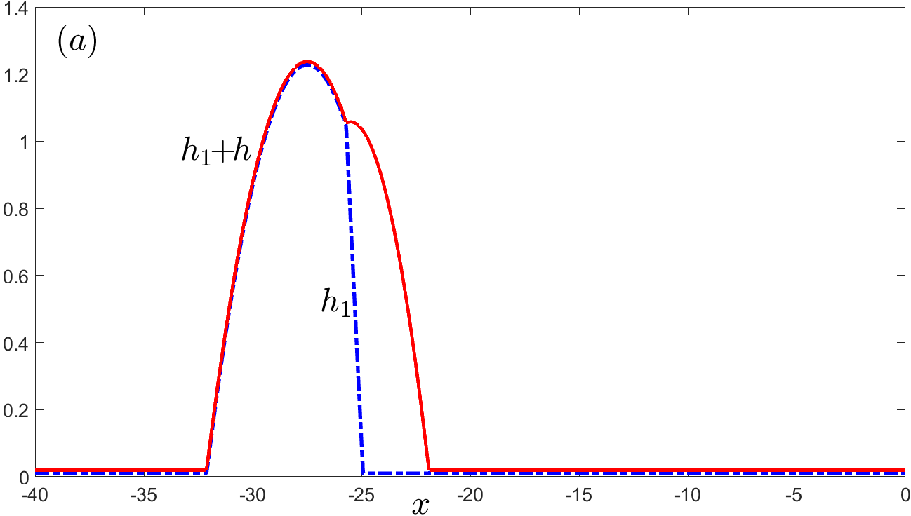
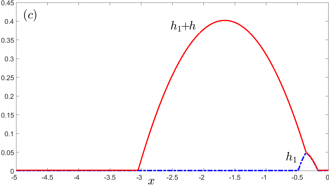
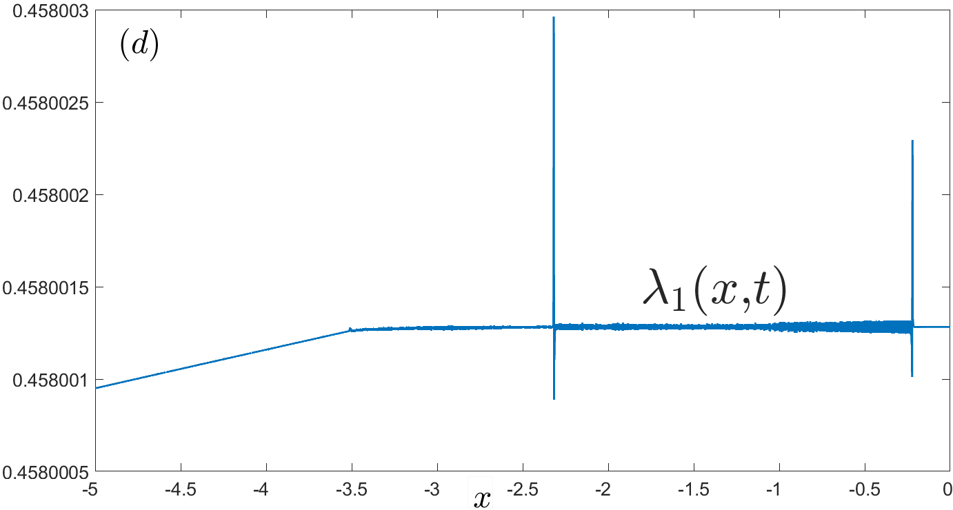
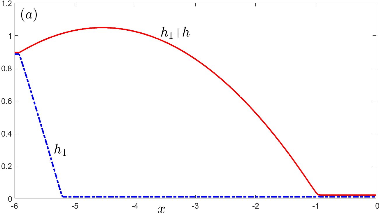
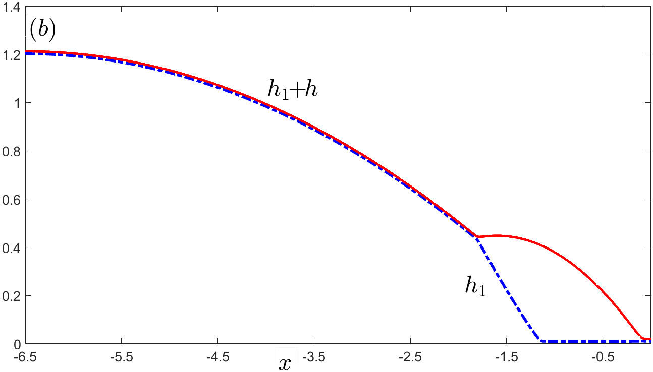
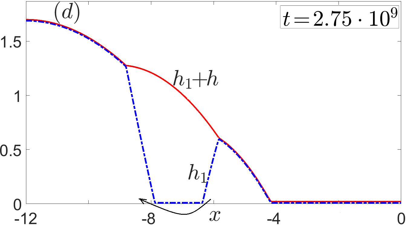
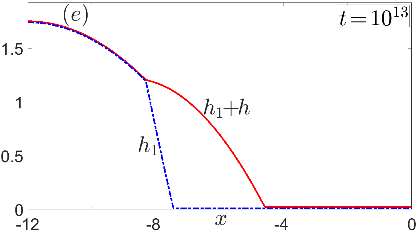
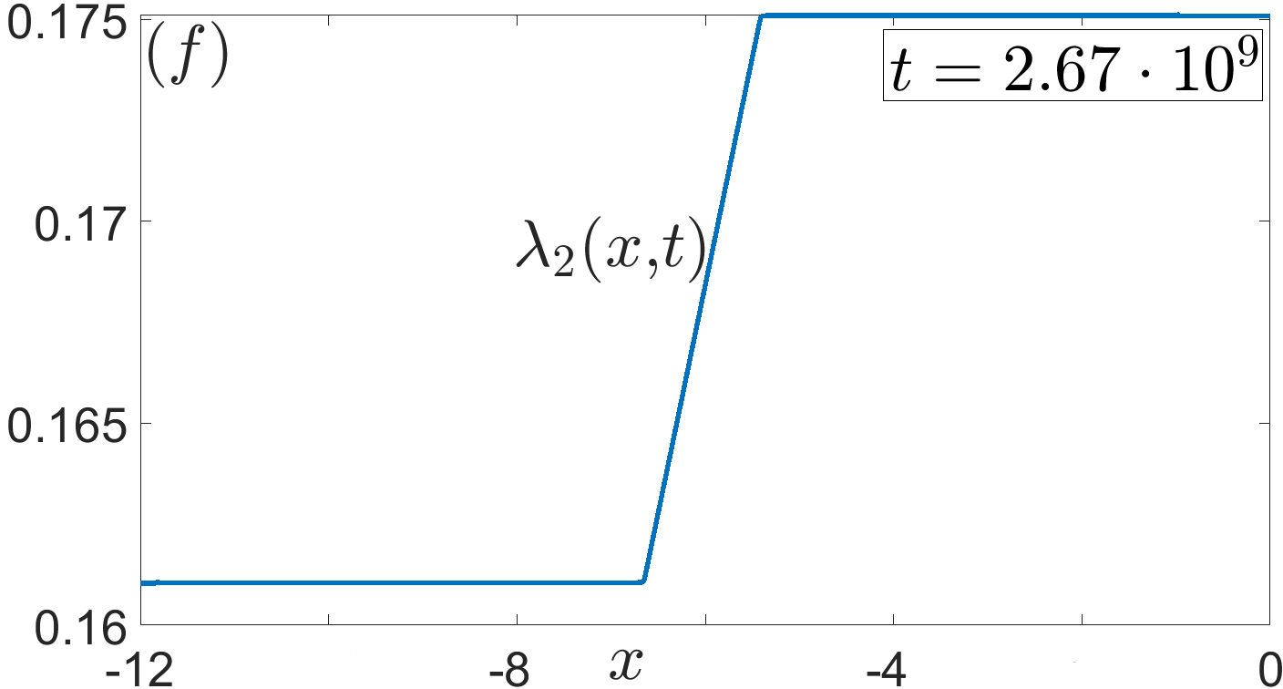
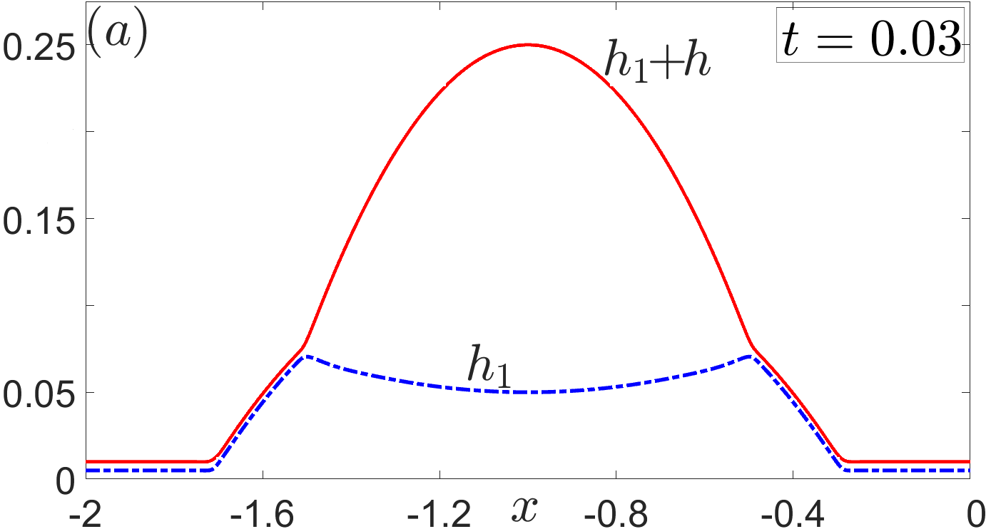
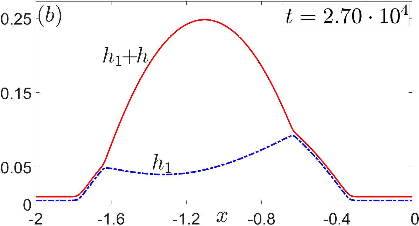
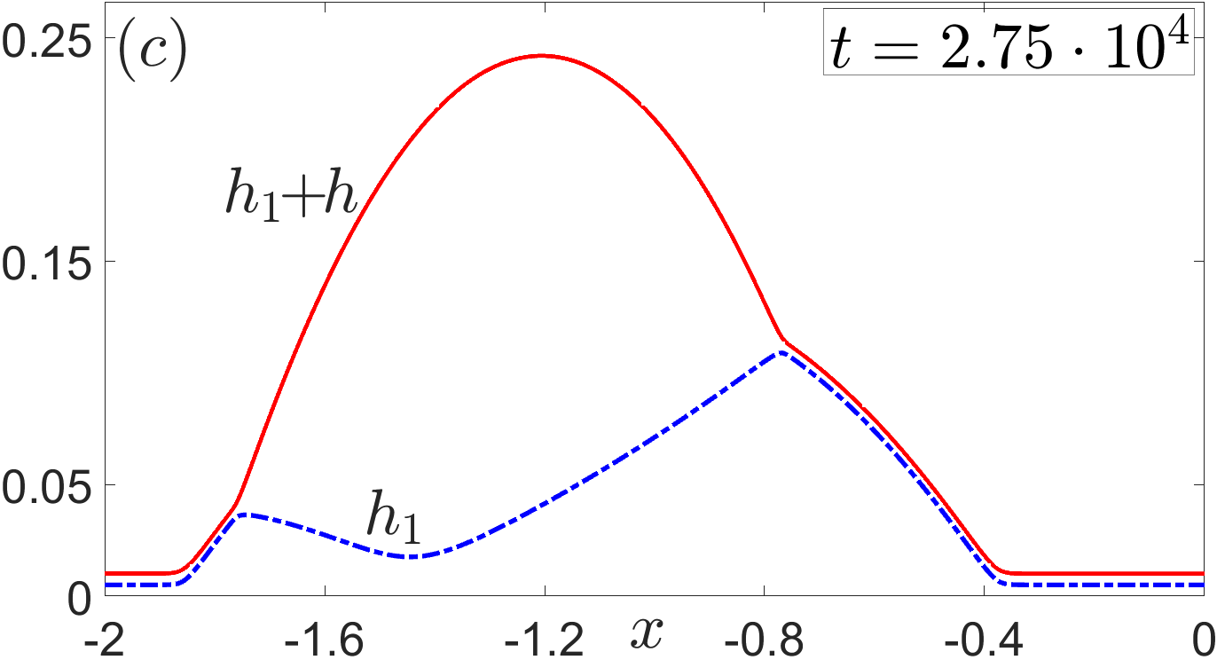
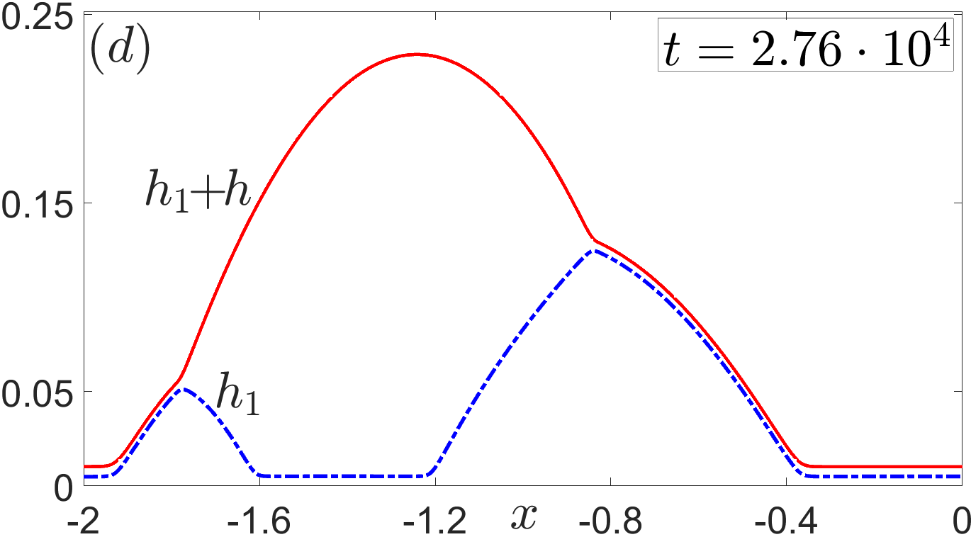
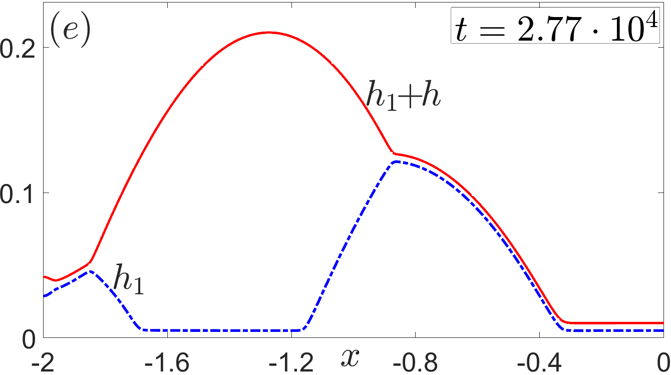
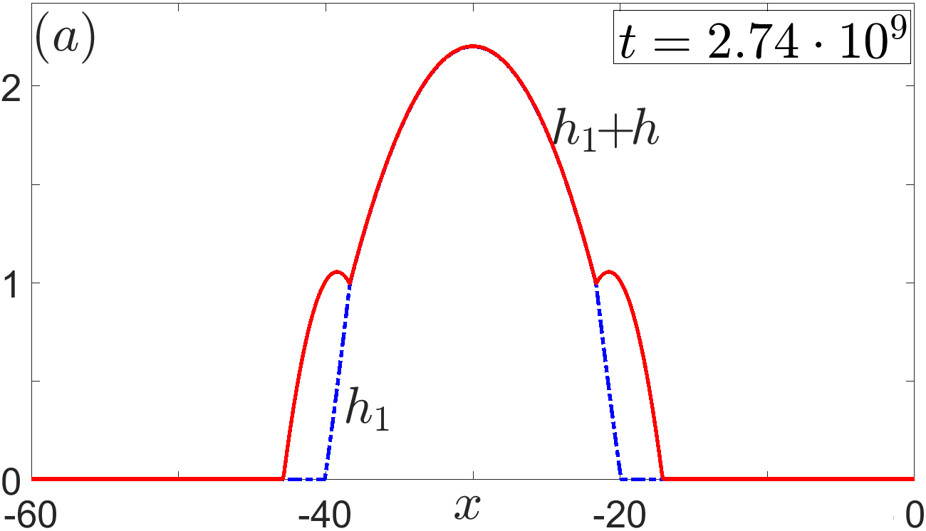
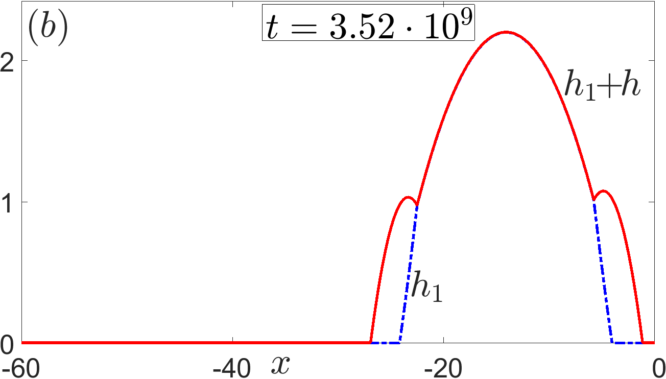
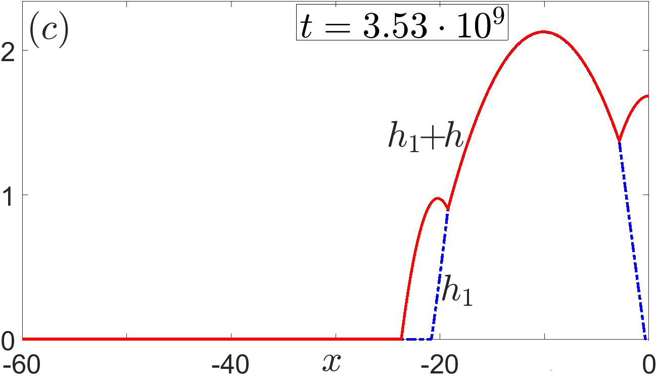
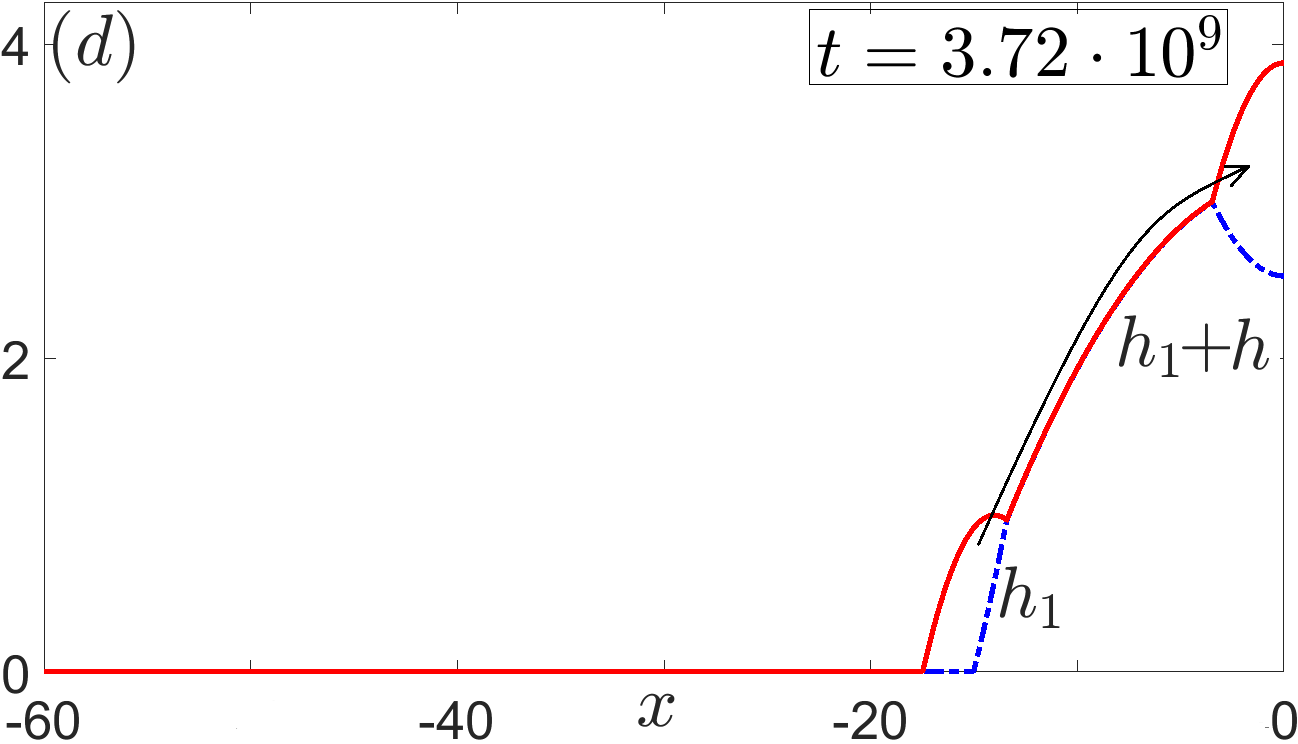
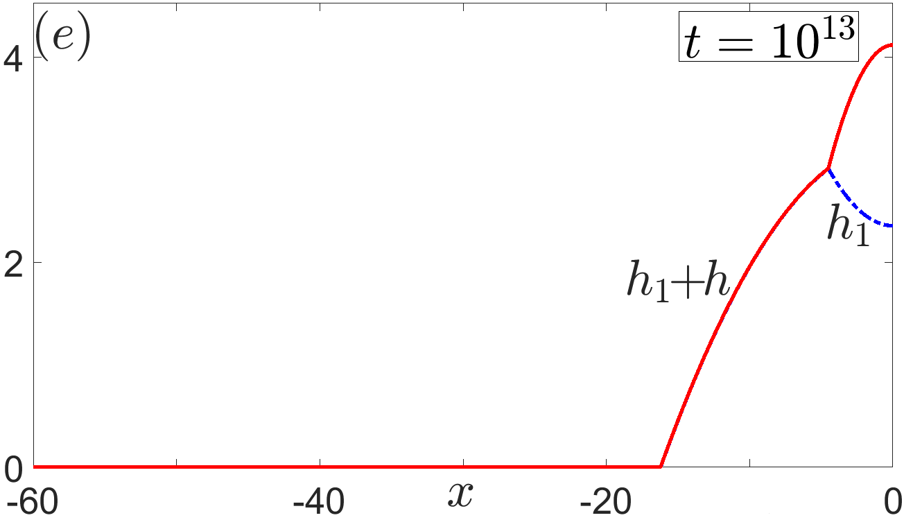
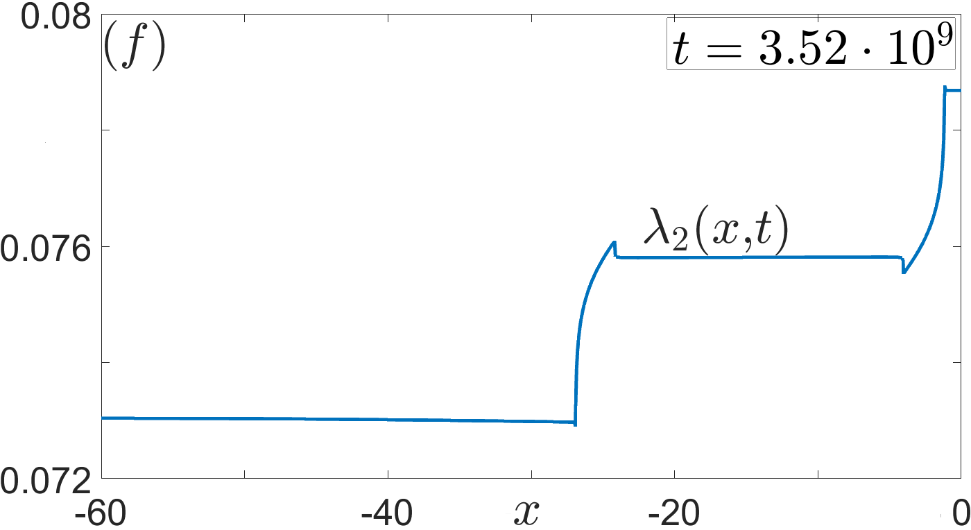
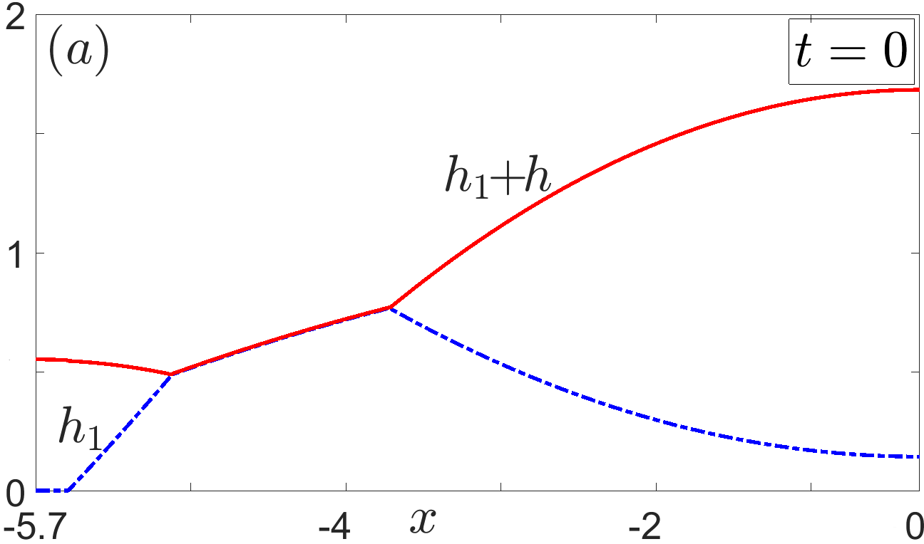
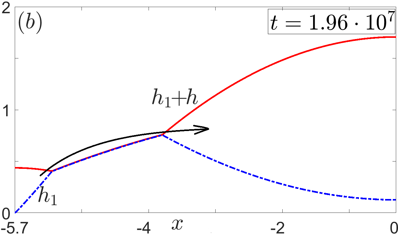
Figure 14: (a)–(e): different time snapshots for coarsening numerical solution to (1)–(4) considered with . Initial condition (5) is symmetric -sessile zig-zag solution to stationary system (8a)–(8c). (f): numerical pressure profile for (b).
The main result of this section is to provide a numerical evidence that other composite solutions (beside the ones described in sections 3–4 and 6) are dynamically unstable when considered as initial profiles (5) for system (1)–(4). For that, firstly, we demonstrate using simulations presented in Fig.14-16 that all symmetric versions of the solutions introduced in sections 3-6, namely those that are obtained by reflection around boundaries or , turn out to be numerically unstable when set as initial profiles (5) for (1)-(4).
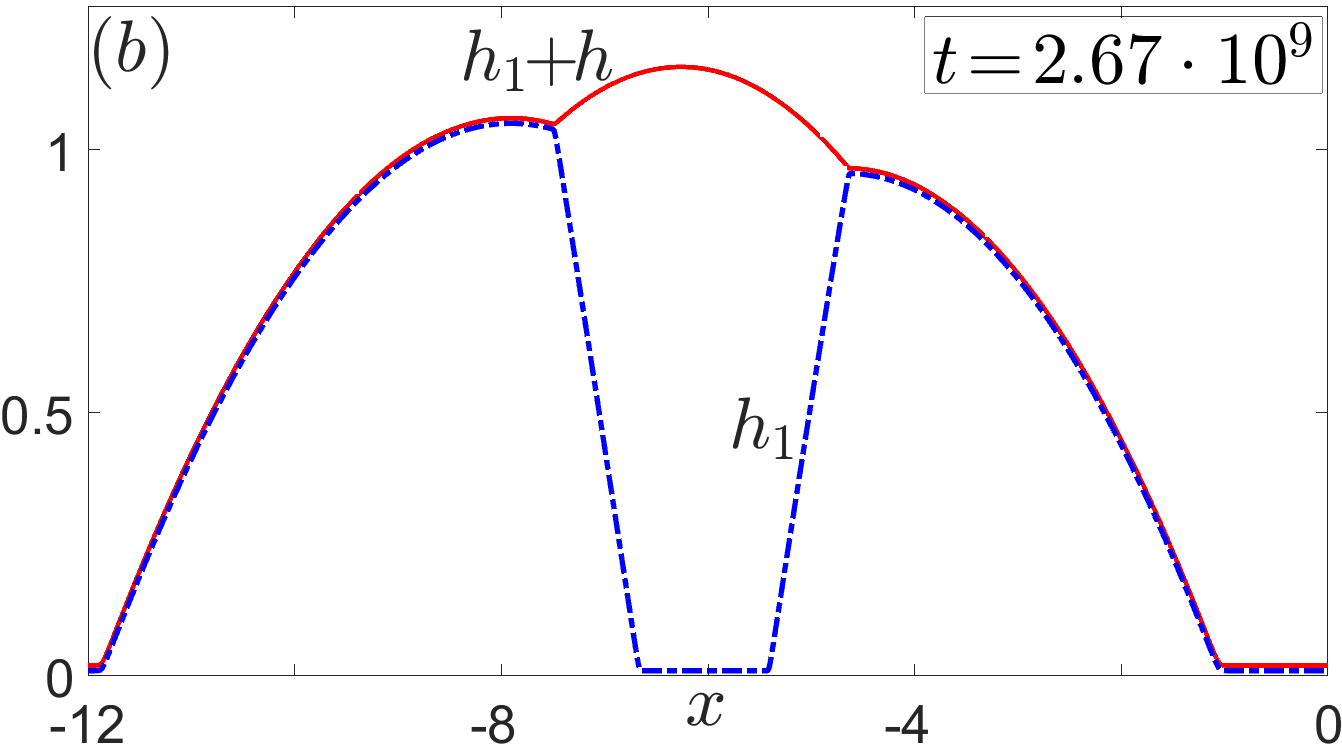
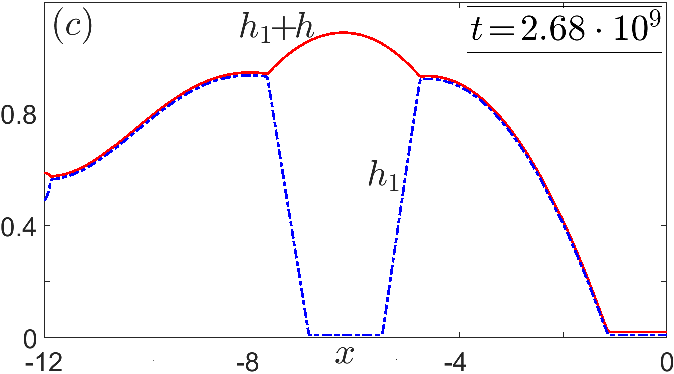
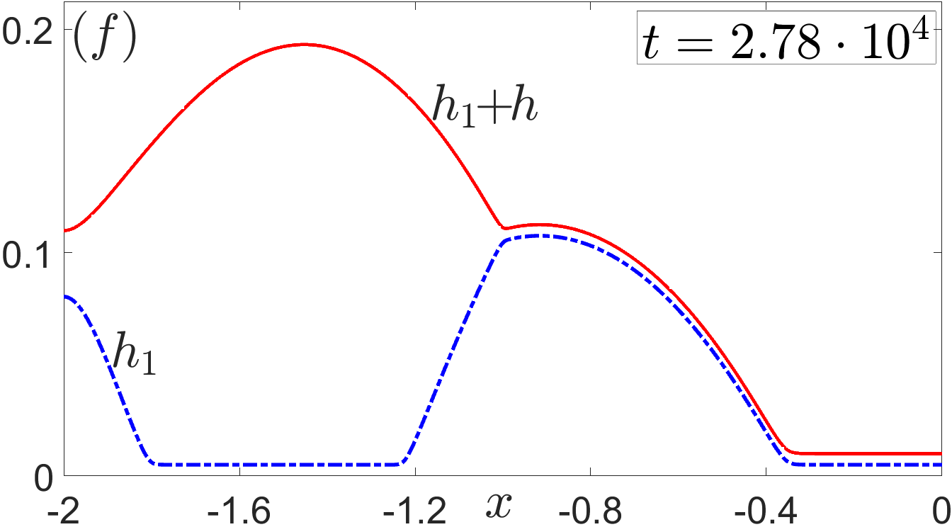
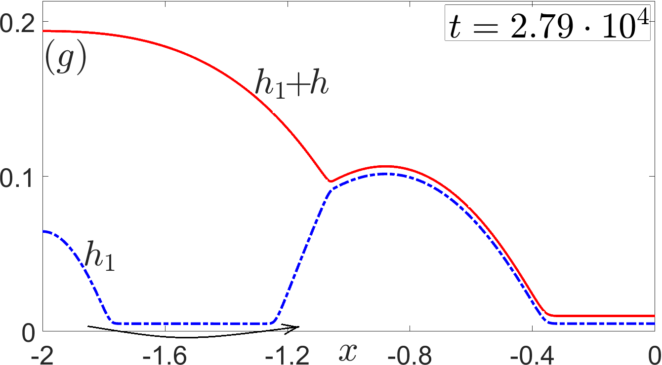
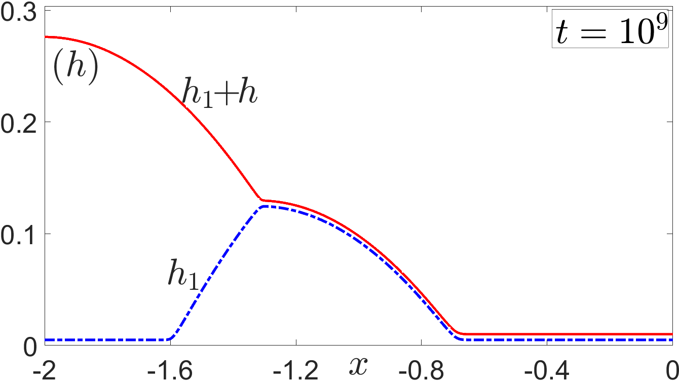
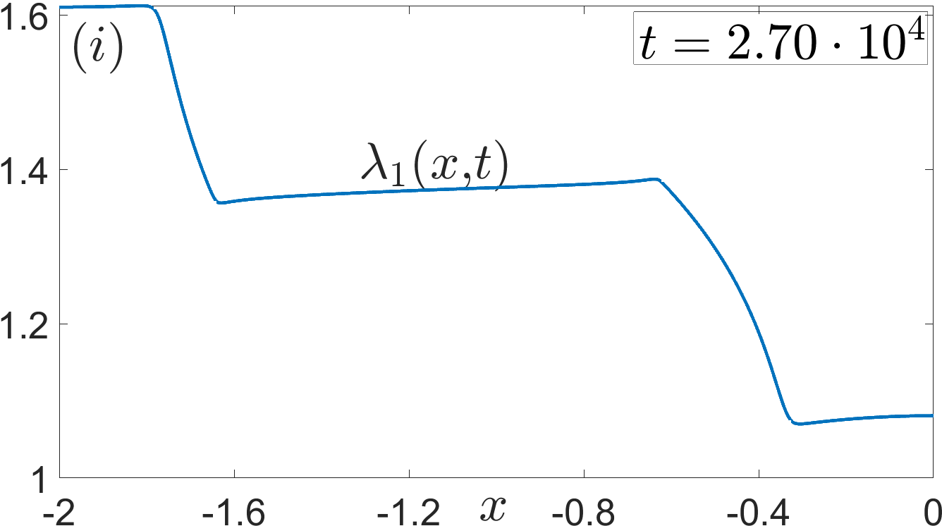
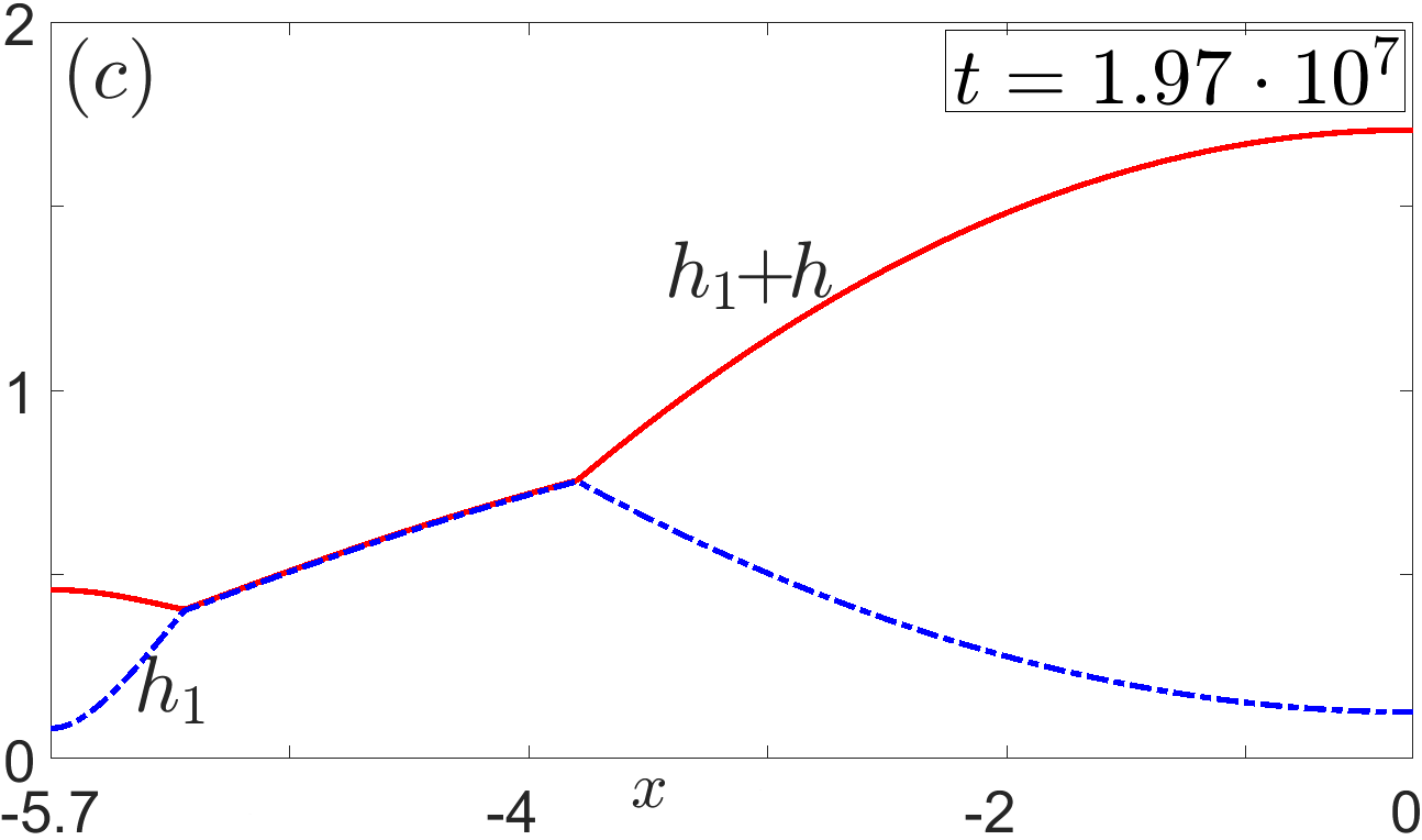
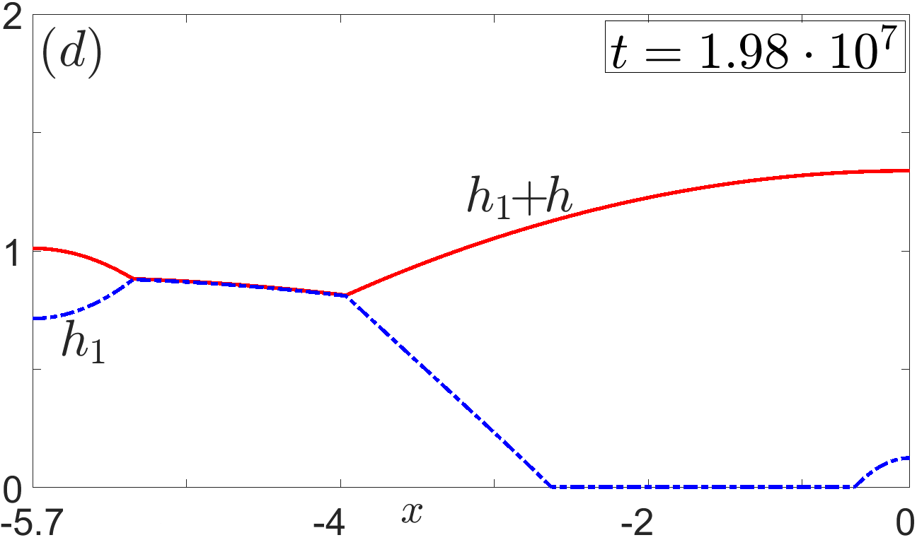
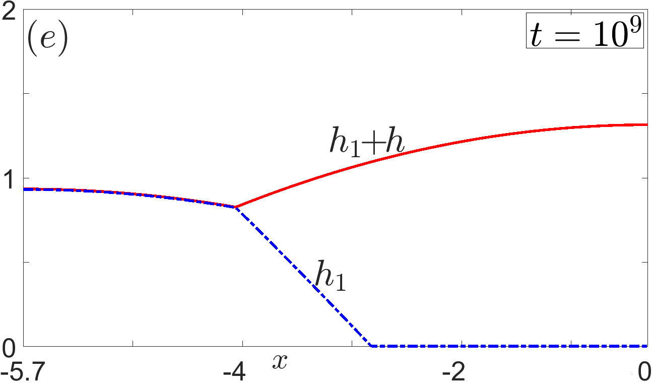
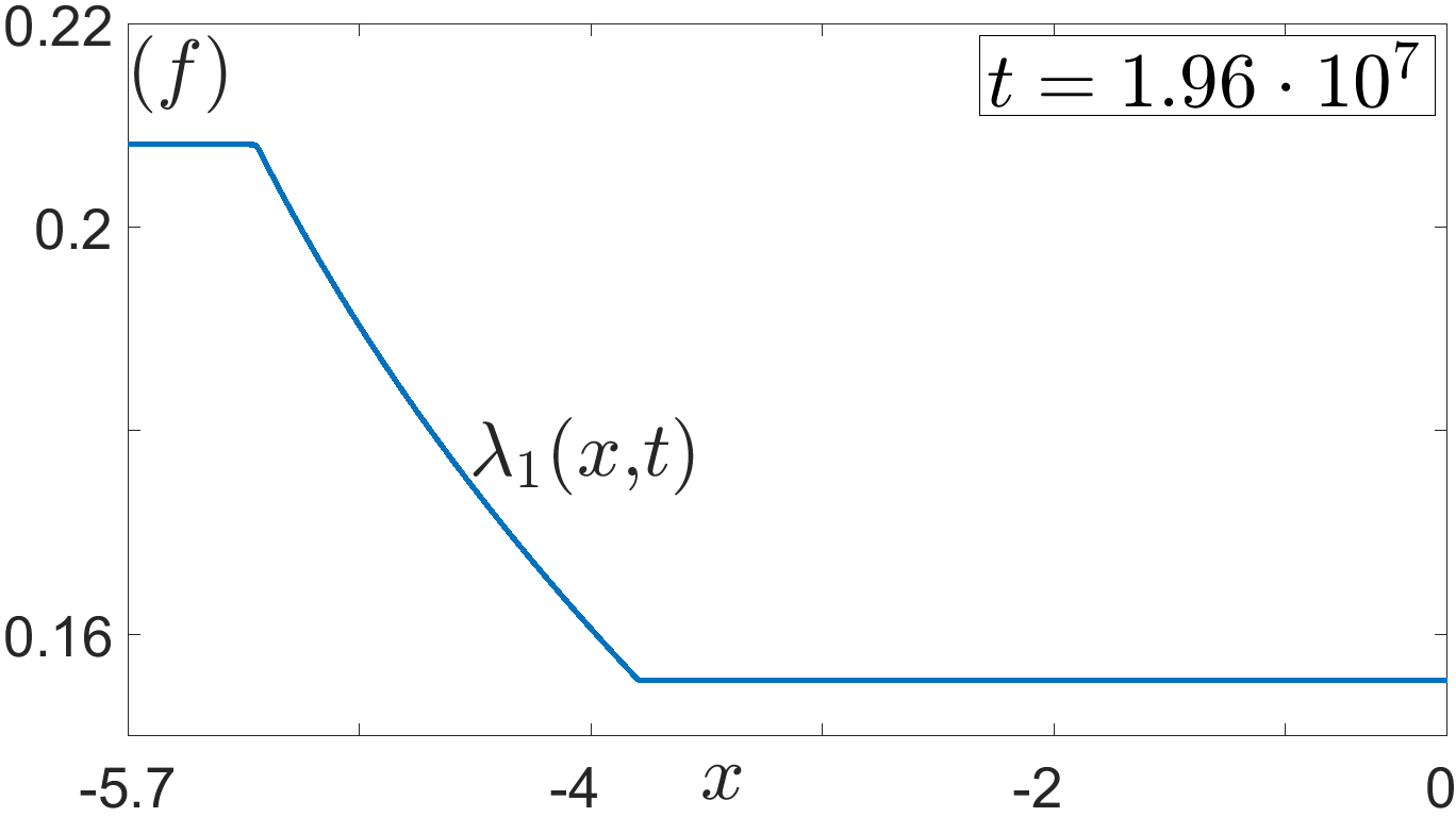
In Fig.14, we take as initial condition (5) a symmetric version of -sessile zig-zag solution abbreviating as () and having six CLs, with its center located at . The corresponding numerical solution to system (1)–(4) exhibits coarsening characterized by a drift of the composite drop to and profound symmetry break of its shape (cf. Fig.14 (b)). Due to that pressure profile (cf. Fig.14 (f)) becomes non-constant and shows small magnitude but profound spatial variation in the middle region (where ) of the composite drop. Such pressure variations are also typical for the coarsening dynamics observed in single layer thin liquid films [11, 12]. Moreover, after the boundary touch a new small lens subdrop nucleates at (cf. Fig.14 (c)) and collapses after relatively short time while, subsequently, a new composite five-CL solution forms. Finally, coarsens in layer via the induced mass flux (depicted by an arrow in Fig.14 (d)) from the smaller bulk region towards the larger one and converges in the long time to stationary -sessile zig-zag solution (cf. Fig.14 (e)).
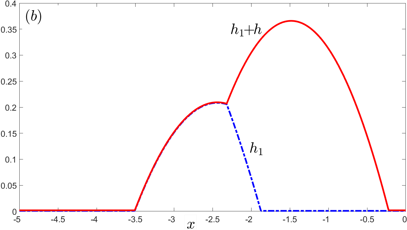
In Fig.15, initial profile (5) is a symmetric version of sessile lens abbreviating as and having four CLs, with its center located at . Again the corresponding numerical solution to (1)–(4) coarsens, drifts to and exhibits profound symmetry break of its ’lens with a collar’ like shape (cf. Fig.15 (a)-(c)). By that pressure profile is non-constant and exhibits two jumps at the collar lateral sides (cf. Fig.15 (i)). Next, the collar breaks into two internal drops (cf. Fig.15 (d)) and after subsequent boundary touch the whole compound drop quickly reforms its layer (cf. Fig.15 (e)–(g)) yielding a composite four-CL solution .
Figure 15: (a)–(h): different time snapshots of coarsening numerical solution to (1)–(4) considered with . Initial condition (5) is symmetric sessile lens solution to stationary system (8a)–(8c). (i): numerical pressure profile for (b).
Finally, coarsens via the induced mass flux in layer (depicted by an arrow in Fig.15 (g)) from the smaller internal drop towards the larger one and converges in the long time to stationary -sessile zig-zag (cf. Fig.15 (h)).
In Fig.16, initial profile (5) is a symmetric version of -sessile zig-zag solution () having six CLs. The corresponding numerical solution to system (1)–(4) coarsens by drifting to and showing small symmetry break of its shape (cf. Fig.16 (b)) reflected by non-constant pressure profile with two jumps in the regions of two lateral drops (cf. Fig.16 (f)). After the boundary touch a new lens subdrop nucleates at (cf. Fig.16 (c)-(d)) and a four-CL solution is formed. Finally, the latter coarsens via the induced mass flux in layer (depicted by an arrow in Fig.16 (d)) from the small lateral drop towards the lens and converges to stationary -sessile lens (inverted in variable) (cf. Fig.16 (e)).
From the simulations presented in Fig.14–16 we conclude that whenever a composite stationary solution to (1)-(4) contains as its part a reflected elementary one-CL one the former is unstable under small perturbations and coarsens via
the induced mass flux in either or layer having thickness. Typical such examples are coarsening of five-CL solution (the reflected part is ) in Fig.14 (d)–(e); four-CL one (the reflected part is ) in Fig.15 (g)–(h); and four-CL one (the reflected part is )) in Fig.16 (d)–(e).
Simulations shown in Fig.17 independently confirm the fact that other composite solutions (beside the eleven ones considered in sections ) are dynamically unstable. In Fig.17 (a), we first derived the leading order profile for
three-CL
Figure 16: (a)–(e): different time snapshots of coarsening numerical solution to (1)–(4) considered with . Initial condition (5) is symmetric -sessile zig-zag solution to stationary system (8a)–(8c). (f): numerical pressure profile for (b).
composite solution to stationary system (8a)–(8c) and then set it as initial condition (5) for system (1)–(4). Note that this composite solution can be obtain by asymptotic matching of zig-zag and lens ones at the CL and the resulting system of the leading order matching conditions, in fact, decouples. Accordingly, for pressures and obey formulae (39)–(40) with and being the maximum of the parabolic profile in the internal region where . Also the positions of the first two CLs for are given by zig-zag expressions (36) (up to replacement there) and, additionally, the following three parameters describe the lens part in Fig.17 (a):
The corresponding numerical solution to (1)–(4) with (5) given by thus described leading order profile of exhibits coarsening due to the induced flux in -layer (depicted by an arrow in Fig.17 (b)) reflected by the pressure variations (cf. Fig.17 (f)). By that the zig-zag part is transformed into a small lens, while at the same time the large one touches and spreads over the substrate with a small internal drop being formed at (cf. Fig.17 (b)–(d)). In the long time both the small lens and internal drop are absorbed into the bulks and the solution converges to stable stationary zig-zag (inverted in variable) one (cf. Fig.17 (e)).
9Discussion
The results of this study lay a mathematical background and provide insight for understanding of the shapes and structure of solutions to the liquid bilayer models considered in [27, 4, 26, 31, 32] and potentially to some recently developed ones [1, 14, 34, 33]. Here we derived explicit formulae for the leading order profiles of eleven types of stationary solutions to one-dimensional bilayer system (1)–(5)
Figure 17: (a)–(e): different time snapshots of coarsening numerical solution to (1)–(4) considered with . Initial condition (5) is composite solution to stationary system (8a)–(8c). (f): numerical pressure profile in (b).
considered with intermolecular potential (2) depending on both layer heights. These solutions were asymptotically matched as compositions of several elementary ones with triple phase contact lines. Numerically solving (1)–(5) we showed that most of these solutions are dynamically stable or weakly translationally unstable. Still other composite stationary solutions to (1)–(5) turn out to be numerically unstable and experience slow time coarsening accompanied by the complex morphological transformations (cf. Fig.14–17).
Interestingly, our results stay in a good correspondence with the observations collected by modeling and experimental studies of thin bilayer systems [27, 4, 26, 31, 32]. In [27], authors produced several experiments with deposition of two immiscible fluid (typically mercury and water) on a hydrophilic glass substrate and observed four types of compound sessile drops, which they termed as encapsulated, lens, collar and Janus ones (cf. Fig.1 of [27]). Some of the found solutions to (1)–(5) partially resemble the two-dimensional compound drop shapes shown in [27, 26] despite the fact that the models used in the latter articles are sharp interface ones explicitly not accounting for possible intermolecular interactions in the experimental setups. Indeed, our internal drop solutions are similar to the encapsulated ones of [26], lens solutions look the same as in [27], our three type of sessile zig-zags resemble well the Janus drops shapes, and a collar type solution is observed in Fig.15. Mathematically seen we prefer to distinguish between sessile and bulk type solutions, because solving the leading order systems of matching conditions for them proceeds differently (e.g. compare solution algorithms to systems (35) and (60) for zig-zag and 2-side sessile zigzag in sections ).
Next, by comparing the coarsening patterns of section with the ones presented and analyzed for one-dimensional bilayer systems in [31, 32] we confirm the presence of two driving coarsening modes observed there: varicose or lens (cf. Fig. 16) and zig-zag (cf. Fig. 14) ones, as well as possible transitions between them (cf. Fig. 17). Besides, we observed a new coarsening mode (not reported in [31, 32]) associated with formation and interaction of internal drops (cf. Fig.15 (f)-(h) and Fig.17 (d)-(e)). Appearance of this new coarsening mode might be connected with our choice of algebraic decay rates in the repulsive terms of intermolecular potential (3).
We conclude the article by stating several interesting open questions:
(a)
For and -drop stationary solutions described in section 3 we found that one of two hydrodynamic pressures or can not be determined from their leading order systems of matching conditions, while in numerical simulations of system (1)–(5) they are observed being negative (cf. Fig.4-5). This unconventional observation should be justified from both physical and mathematical sides.
(b)
The method for asymptotic matching of stationary solutions to (1)–(5) presented in sections can be used for constructing the composite ones with any arbitrary number of triple contact lines. Beside the stability one, there exists a question whether the solution existence domains (EDs) in the space of model parameters (similar to those presented in Fig.13 of section ) shrink to empty sets at some finite or not.
(c)
Bifurcation analysis of the stationary solutions to (1)–(5) in the spirit of studies [3, 36] is yet lacking, though the first step towards it is done in diagrams of Fig.13. In particular, our numerical simulations do not reveal solutions with four-phase merging contact lines predicted in [26], which still may belong to unstable bifurcation paths.
(d)
Our results lay mathematical background for further analysis of the coarsening dynamics in bilayer system following similar approaches to those ones developed for one-layer thin film equations [11, 12, 13, 20, 21, 23].
10Acknowledgments
The author would like to thank Dirk Peschka and Barbara Wagner for our stimulating discussion of possible forms for intermolecular potential (2).
References
[1]
M. Areshi, D. Tseluiko, U. Thiele, B. D. Goddard, and A. J. Archer.
Binding potential and wetting behavior of binary liquid mixtures on surfaces.
Phys. Rev. E., 109: 024801, 2024.
[2]
D. Bandyopadhyay, R. Gulabani, and A. Sharma.
Instability and dynamics of thin liquid bilayers.
Ind. Eng. Chem. Res., 44: 1259-1272, 2005.
[3]
A. L. Bertozzi, G. Grün, and T. P. Witelski.
Dewetting films: bifurcations and concentrations.
Nonlinearity, 14(6): 1569-1592, 2001.
[4]
N. Blanken, M. S. Saleem, M. J. Thoraval, and C. Antonini.
Impact of compound drops: a perspective.
Curr. Opin. Colloid Interface Sci., 51: 101389, 2021.
[5]
D. Bonn, J. Eggers, J. Indekeu, J. Meunier and E. Rolley.
Wetting and spreading.
Rev. Mod. Phys., 81: 739-805, 2011.
[6]
R. V. Craster and O. K. Matar.
On the dynamics of liquid lenses.
J. Colloid. Interface. Sci., 303: 503–516, 2006.
[7]
R. V. Craster and O. K. Matar.
Dynamics and stability of thin liquid films.
Rev. Mod. Phys., 81: 1131–1196, 2009.
[8]
K. D. Danov, V. N. Paunov, N. Allerborn, H. Raszillier and F. Durst.
Stability of evaporating two-layered liquid film in the presence of surfactant-I. The equations of lubrication approximation.
Chem. Engin. Sci., 53: 2809-2822, 1998.
[9]
J. Escher and B.-V. Matioc.
Non–negative global weak solutions for a degenerated parabolic system approximating the two–phase Stokes problem.
J. Differ. Equ., 256(8): 2659–2676, 2014.
[10]
L. S. Fischer and A. A. Golovin.
Nonlinear stability analysis of a two-layer thin liquid film: Dewetting and autophobic behavior.
J. Colloid. Interface. Sci., 291: 515–528, 2005.
[11]
K. B. Glasner and T. P. Witelski.
Coarsening dynamics of dewetting films.
Phys. Rev. E, 67: 016302, 2003.
[12]
K. B. Glasner and T. P. Witelski.
Collision vs. collapse of droplets in coarsening of dewetting thin films.
Physica D, 209: 80-104, 2005.
[13]
K. Glasner, F. Otto, T. Rumpf, and D. Slepčev.
Ostwald ripening of droplets: The role of migration
Eur. J. Appl. Math., 20(1): 1-67, 2009.
[14]
S. Hartmann, J. Diekmann, D. Greve, and U. Thiele.
Drops on polymer brushes: advances in thin-film modeling of adaptive substrates.
Langmuir, 40(8): 4001–4021, 2024.
[15]
R. Huth, S. Jachalski, G. Kitavtsev, D. Peschka and B. Wagner.
Gradient flow perspective on thin-film bilayer flows.
J. Eng. Math., 94: 43-61, 2015.
[16]
J. N. Israelachvili.
Intermolecular and surface forces.
Oxford mathematical monographs.
Academic, London 1992.
[17]
S. Jachalski, R. Huth, G. Kitavtsev, D. Peschka and B. Wagner.
Stationary solutions of liquid two-layer thin-film models.
SIAP, 73(3): 1183-1202, 2013.
[18]
S. Jachalski, D. Peschka, A. Münch and B. Wagner.
Impact of interfacial slip on the stability of liquid two-layer polymer films.
J. Eng. Math., 86: 9-29, 2014.
[19]
S. Jachalski, G. Kitavtsev and R. M. Taranets.
Weak solutions to lubrication systems describing the evolution of bilayer thin films.
Commun. Math. Sci., 12(3): 527–544, 2014.
[20]
G. Kitavtsev and B. Wagner.
Coarsening dynamics of slipping droplets.
J. Eng. Math., 66: 271-292, 2010.
[21]
G. Kitavtsev, L. Recke, and B. Wagner.
Centre manifold reduction approach for the lubrication equation.
Nonlinearity, 24: 2347, 2011.
[22]
G. Kitavtsev, L. Recke, and B. Wagner.
Asymptotics for the Spectrum of a Thin Film Equation in a Singular Limit.
SIAM J. Appl. Dyn. Syst., 11(4): 1425-1457, 2012.
[23]
G. Kitavtsev.
Coarsening rates for the dynamics of slipping droplets.
Eur. J. Appl. Math., 25(1): 83-115, 2014.
[24]
G. Kitavtsev, M. Fontelos, and J. Eggers.
Thermal rupture of a free liquid sheet.
J. Fluid Mech., 840: 555-578, 2018.
[25]
J. J. Kriegsmann and M. J. Miksis.
Steady motion of a drop along a liquid interface.
SIAM J. Appl. Math., 64: 18–40, 2003.
[26]
L. Mahadevan, M. Adda-Bedia, and Y. Pomeau.
Four-phase merging in sessile compound drops.
J. Fluid Mech., 451: 411-420, 2002.
[27]
M. J. Neeson, R. F. Tabor, F. Griezer, R. R. Dagastine, and D. Y. Chan.
Compound sessile drops.
Soft Matter, 8: 11042-11050, 2012.
[28]
A. Nepomnyashchy.
Droplet on a liquid substrate: Wetting, dewetting, dynamics, instabilities.
Curr. Opin. Colloid Interface Sci., 51: 101398, 2021.
[29]
A. Oron, S. H. Davis, and S. G. Bankoff.
Long-scale evolution of thin liquid films.
Rev. Mod. Phys., 69(3): 931-980, 1997.
[30]
D. Peschka.
Self-similar rupture of thin liquid films with slippage.
Phd thesis, Humboldt University of Berlin, 2008.
[31]
A. Pototsky, M. Bestehorn, D. Merkt and U. Thiele.
Alternative pathways of dewetting for a thin liquid two-layer film.
Phys. Rev. E, 70: 025201, 2004.
[32]
A. Pototsky, M. Bestehorn, D. Merkt and U. Thiele.
Morphology changes in the evolution of liquid two-layer films.
J. Chem. Phys., 122: 224711, 2005.
[33]
A. Pototsky, A. Oron, and M. Bestehorn.
Equilibrium shapes and floatability of static and vertically vibrated heavy liquid drops on the surface of lighter liquid.
J. Fluid Mech., 922: A31, 2021.
[34]
A. Pototsky and I. S. Maksymov.
Nonlinear periodic and solitary rolling waves in falling two-layer liquid viscous films.
Phys. Rev. Fluids, 8(6): 064801, 2023.
[35]
R. Seemann, S. Herminghaus, and K. Jacobs.
Gaining control of pattern formation of dewetting liquid films.
J. Phys.: Condensed Matter, 13: 4925-4938, 2001.
[36]
Y. Zhang.
Counting the stationary states and the convergence to equilibrium for the 1-D thin film equation.
Nonlinear Anal., 71: 1425-1437, 2009.