Inverse participation ratio and entanglement of edge states in HgTe quantum wells in a finite strip geometry

Abstract

Localization and entanglement properties of edge states of HgTe quantum wells in a finite strip geometry of width $L$ are studied under quantum information concepts such as: 1) inverse participation ratio (IPR), which measures localization, and 2) entropies of the reduced density matrix (RDM) for the spin sector, which measures quantum correlations due to the spin-orbit coupling (SOC). Qualitative and quantitative information on the edge states energies and wavefunctions is extracted from analytic and numerical Hamiltonian diagonalization approaches. The previously observed exponential decay of the energy gap with $L$ and its modulations is confirmed and nontrivial consequences of the strip width and Rashba terms on the charge conductance are also reviewed. Analysis of the structure of the edge-state wave functions in terms of spin, momentum $k_{x}$ in the $x$-direction and position $y$, evidences the spin polarization structure of edge states at the boundaries. An IPR analysis reveals that the valence edge states show maximum localization on the boundaries for certain values of the momenta $k_{x}$ in the vicinity of the $\Gamma$ point. The edge-state wave packets participate of less and less momenta as we approach to the boundaries $y=0,L$ (and also the center $y=L/2$, for some of them) of the strip. A study of the RDM to the spin sector of edge states sheds complementary information on the structure of spin probabilities in $(k_{x},y)$ space, giving clear location of extremal values. The purity and entropies of the RDM inform on the regions $(k_{x},y)$ where the spin sector is more and less entangled with the rest of the system, due to SOC.

I Introduction

The spin Hall (SH) effects are associated to relativistic spin-orbit couplings in which electric currents can generate spin currents or viceversa. See e.g. [1], and references there in, for a review of the SH effects and its development to have spintronic devices. The SH effect can be intrinsic (due to the structure of the electronic bands) or extrinsic (due to scattering process), both emerging naturally from the formalism of the anomalous spin Hall (ASH) effect, which generates asymmetric deflections of charge carriers depending on its spin direction [2]. The so-called intrinsic spin Hall effect (ISH) combined with the quantum Hall effect (QH) led to the prediction and subsequent experimental verification of the quantum spin Hall (QSH) effect.

The QSH state is a non-trivial topological state of quantum matter which is invariant under time reversal transformations (see e.g. [3] for a review). It has an energy gap in the bulk, but it has edge states with different spins moving in opposite directions, that is, counter-propagating modes at each edge. These spin currents flow without dissipation on macroscopic scales. Mathematically motivated by an earlier model of Haldane [4], graphene was proposed by Kane & Mele as a two dimensional (2D) Dirac material to exhibit this effect [5, 6], however the spin currents were too small to be measurable. Another proposal made by Bernevig-Hughes-Zhang (BHZ) [7, 8], considering the mercury telluride-cadmium telluride semiconductor quantum wells (QW), was successful and this new QSH state of matter and spin polarization phenomena were experimentally confirmed through the observation of ballistic edge channels [9, 10] and by electrical detection [11]. The intrinsic QSH effect can be switched on and off and tuned into resonance through the manipulation of the QW width, or the bias electric field across the QW [12]. Since these pioneering studies, many low-dimensional quantum spintronic devices based on the spin-polarized transport in HgTe/CdTe QWs, and other non-magnetic semiconductors, have been proposed (see e.g. [13]). For example, other QWs exhibiting a similar behavior to HgTe/CdTe are the so-called type-II semiconductors made from InAs/GaSb/AlSb, which have been studied in [14], where they suggest to use this system to construct a QSH field effect transistor (FET).

The QSH phenomenom was extended to 3D topological insulators (TI); see [15, 16, 17] for text books and [18, 19] for standard reviews on TI. In this case, surface states arise with high conductivity properties, like the alloy Bi_x Sb_1-x, which exhibits 2D conducting surface states. Effective Hamiltonian models have been proposed to describe this surface states of 3D TI [20, 21, 22].

To study the finite size effects on edge states in the TI phase, there are two procedures in the current literature. On the one hand, the tight-binding method is used in the works about the QSH edge-states by [5, 6, 23, 24, 25]. On the other hand, an analytic procedure of the effective BHZ model Hamiltonian for the case of a finite strip geometry was given in [26, 24]; here the expressions of the wave functions of the edge states are determined in analytic form. Due to the finite size of the sample, the good quantum number $k_{y}$ (the wavevector component in the finite strip direction) is replaced by a complex number $\lambda$ leading to localization properties of wavefunctions at the boundaries and, as a consequence, to the coupling interaction between the edge states, thus producing an energy gap.

In this paper, we tackle the problem of finite size effects in the HgTe/CdTe semiconductors, including spin-orbit effects due to bulk- and structure-inversion asymmetries (resp. BIA and SIA). This problem has also been investigated in [25], where they use the tight-binding method to determine and exponential decay of the energy gap (with oscillations) with the strip width $L$ and to prove that this gap is not localized at the $\Gamma$ point of the first Brillouin zone. This energy gap is also affected by an external perpendicular electric field, which tunes the Rashba (SIA) term of the Hamiltonian model. We confirm this behavior for a more general BIA term including extra electron and hole couplings preserving time reversal symmetry. We also pursue the identification of topological order through quantum information (QI) measures and concepts like entropy and entanglement. These tools have played an important role in the general understanding of quantum phase transitions. Indeed, entanglement is at the heart of the interplay between quantum information and quantum phases of matter (see e.g., [27, 28]). Signatures of topological phase transitions in higher Landau levels of HgTe/CdTe quantum wells without SOC from an information theory perspective have been reported in [29]. Other localization measures, like the inverse participation measure (IPR), has given useful information about the topological phase transition 2D Dirac materials like silicene [30]. This paper analyzes the structure of edge states in HgTe QWs with SOC under QI concepts like IPR and entanglement entropy, which turn out to be an interesting “microscope” to reveal details of their internal structure.

The organization of the paper is as follows. In Sec. II we briefly discuss the structure of the HgTe QW Hamiltonian model and its topological phases. In Sec. III we approach the analysis of edge states in a finite strip geometry of width $L$ from two different perspectives: either looking for analytic localized eigenvectors of the low energy Hamiltonian, or by numerically solving the tight-binding model after a lattice regularization. The first approach gives us a deeper understanding of the qualitative and internal structure of edge states, but shall rather follow the second approach to extract quantitative information, firstly about the spectrum and the dependence of the energy gap on the strip width $L$ and the Rashba coupling $\xi$, and its non-trivial consequences on the charge conductance of edge states and its potential use in the design of a QSH field effect transistor. In Sec. IV we take a closer look to the localization properties of edge states as a function of the spin ($s=\pm 1$), the momentum wave vector in the $x$-direction [$k_{x}\in(-\pi/a,\pi/a)$, with $a$ the lattice constant] and the position $y\in[0,L]$ between the strip boundaries $y=0,L$. This study sheds light on the spin polarization structure of edge states at the boundaries. The spreading of edge states in momentum ($k_{x}$) and position ($y$) space is analyzed through an important quantum information (and statistical, in general) concept called “inverse participation ratio” (IPR). Finally in Sec. V we use the reduced density matrix (RDM) to the spin subsystem to analyze spin up/down and spin transfer probability densities of edge states as a function of the momentum $k_{x}$ and position $y$, paying especial attention to extremal values. This analysis also sheds light on the spin polarization structure of edge states. The purity of the RDM (or equivalently, the linear entropy) also gives us information about the degree of entanglement between spin and band (electron-hole) sectors. Extremal entanglement values occur for special values of the position $y$ and momentum $k_{x}$. Other alternative correlation measures are also analyzed, all of them giving equivalent results. Finally, Sec. VI is devoted to conclusions.

II Model Hamiltonian

Following standard references like [31, 7, 9, 24, 19, 32], edge states in HgTe/CdTe QWs are described by the following 2D four-band effective Dirac Hamiltonian. The original BHZ Hamiltonian is

$$H_{\mathrm{BHZ}} = \frac{\sigma_{0}+\sigma_{z}}{2}\otimes h_{+1}+\frac{\sigma_{0}-\sigma_{z}}{2}\otimes h_{-1},$$

$$h_{s}(\bm{k}) = \epsilon_{0}(\bm{k})\sigma_{0}+\bm{d}_{s}(\bm{k})\cdot\bm{\sigma},\,s=\pm 1,$$

where $\bm{\sigma}=(\sigma_{x},\sigma_{y},\sigma_{z})$ are Pauli matrices together with the $2\times 2$ identity matrix $\sigma_{0}$ and $\bm{k}=(k_{x},k_{y})$ is the wavevector. The spin $s=\pm 1$, $2\times 2$ matrix Hamiltonians $h_{s}(\bm{k})$ are related by $h_{-1}(\bm{k})=h_{+1}^{*}(-\bm{k})$ (temporarily reversed) and they admit an expansion around the center $\Gamma$ of the first Brillouin zone (FBZ) given by [7],

$$\epsilon_{0}(\bm{k})=\gamma-\delta\bm{k}^{2},\quad\bm{d}_{s}(\bm{k})=(\alpha sk_{x},-\alpha k_{y},\mu-\beta\bm{k}^{2}),$$ (1)

where $\alpha,\beta,\gamma,\delta$ and $\mu$ are material parameters that depend on the HgTe QW geometry, in particular on the HgTe layer thickness $\ell$. The parameter $\gamma$ can be disregarded and we shall set it equal to zero in the following. In Table 1) we provide these material parameters for a HgTe layer thickness $\ell=7$ nm. We shall use these values all along the manuscript unless otherwise stated.

Edge states are topologically protected by the time reversal symmetry

$$\Theta=-i(\sigma_{y}\otimes\sigma_{0})K,$$ (2)

where $K$ means complex conjugation. The $\mathrm{sign}(\mu)=\mathrm{sign}(\ell_{c}-\ell)$ of the mass or gap parameter $\mu$, for a given HgTe layer thickness $\ell$, differentiates between band insulator ($\ell<\ell_{c}$) and topological insulator ($\ell>\ell_{c}$) phases, with $\ell_{c}\simeq 6.3$ nm the critical thickness. The QSH phase is associated with a discrete $\mathbb{Z}_{2}$ topological invariant [33]. Actually, the Thouless-Kohmoto-Nightingale-Nijs (TKNN) formula provides the Chern-Pontryagin number

$$\mathcal{C}_{s}=\frac{1}{2\pi}\int\int_{\mathrm{FBZ}}d^{2}\bm{k}\left(\frac{\partial\hat{\bm{d}}_{s}(\bm{k})}{\partial k_{x}}\times\frac{\partial\hat{\bm{d}}_{s}(\bm{k})}{\partial k_{y}}\right)\cdot\hat{\bm{d}}_{s}(\bm{k}),$$ (3)

with $\hat{\bm{d}}_{s}=\bm{d}_{s}/|\bm{d}_{s}|$, which gives

$$\mathcal{C}_{s}=s[\mathrm{sign}(\mu)+\mathrm{sign}(\beta)],$$ (4)

so that the system undergoes a topological phase transition (TPT) from normal ($\ell<\ell_{c}$ or $\mu/\beta<0$) to inverted ($\ell>\ell_{c}$ or $\mu/\beta>0$) regimes at the critical HgTe layer thickness $\ell_{c}$.

Now we shall introduce spin-orbit coupling (SOC) that connects the spin blocks $h_{\pm 1}$. It is given by the Hamiltonian

$$H_{\mathrm{SOC}} = H_{\mathrm{BIA}}+H_{\mathrm{SIA}},$$ (5)

$$H_{\mathrm{BIA}}(\bm{k}) = \Delta_{z}(\sigma_{y}\otimes\sigma_{y})$$

$$+\frac{\Delta_{e}}{2}(k_{x}\sigma_{x}-k_{y}\sigma_{y})\otimes(\sigma_{0}+\sigma_{z})$$

$$+\frac{\Delta_{h}}{2}(k_{x}\sigma_{x}+k_{y}\sigma_{y})\otimes(\sigma_{0}-\sigma_{z}),$$

$$H_{\mathrm{SIA}}(\bm{k}) = \mathrm{i}\frac{\xi}{2}(k_{x}\sigma_{x}+k_{y}\sigma_{y})\otimes(\sigma_{0}+\sigma_{z}).$$

The spin-orbit interaction creates a bulk inversion asymmetry (BIA) and a structural inversion asymmetry (SIA) term which manifests as a $k$-linear Rashba term proportional to $\xi$ for the electron band (see e.g. [14, 24, 34, 32]); a finite Rashba term of this type in HgTe QWs requires the presence of a non-zero electric field $\mathcal{E}_{z}$ in the $z$ direction, so that $\xi\propto e\mathcal{E}_{z}$, with $e$ the electric charge. We shall set $\mathcal{E}_{z}=1$ mV/nm all along the manuscript, except for the discussion of the variation of the charge conductance with $\xi$ towards the end of Sec. III and Fig. 4.

The spin-orbit interaction $H_{\mathrm{SOC}}$ will be responsible for the entanglement between spin blocks of $H_{\mathrm{BHZ}}$ in the total Hamiltonian

$$H=H_{\mathrm{BHZ}}+H_{\mathrm{SOC}}.$$ (6)

Notice that we are arranging Hamiltonian basis states as 4-spinor column vectors of the form

$$\Psi=(\psi_{\uparrow E},\psi_{\uparrow H},\psi_{\downarrow E},\psi_{\downarrow H})^{T},$$ (7)

where $\uparrow,\downarrow$ makes reference to the spin degree of freedom $s=\pm 1$ and $EH$ denotes the electron and hole bands, respectively.

The introduction of $H_{\mathrm{SOC}}$ preserves the time reversal symmetry of the total Hamiltonian $H$ and therefore does not affect the topological stability of the nontrivial insulator phase already discussed for $H_{\mathrm{BHZ}}$. We shall set $\ell=7$ nm and we shall analyze the topological insulator phase for the material parameters given in table 1. To enhance some physical behavior, due to finite size effects, we shall occasionally consider other values of $\Delta_{z}$, which will be noted in due course.

$\alpha$	$\beta$	$\delta$	$\mu$
(meV.nm)	(meV.nm2)	(meV.nm2)	(meV)
365	-686	-512	-10

$\Delta_{e}$	$\Delta_{h}$	$\Delta_{z}$	$\xi/|e\mathcal{E}_{z}|$
(meV.nm)	(meV.nm)	(meV)	(nm2)
-12.8	21.1	1.6	15.6

Table 1: Values of the HgTe/CdTe QW material parameters for a HgTe layer thickness of $\ell=7$ nm [19, 32].

III Energy gap for edge states in a finite strip geometry

In order to extract qualitative and quantitative information on edge states, we shall report on two different but complementary approaches to the solution of the Hamiltonian eigenvalue problem.

III.1 Analytic approach to the solution of the effective continuous 4-band model

Following Ref. [26] (see also [22] for 3D Bi₂Se₃ films grown on a SiC substrate), the general solution for edge states in a finite strip geometry can be derived analytically as follows. We chose the boundaries of the sample to be perpendicular to the $y$-axis. Four-spinor states $\Psi(y)=\Psi_{\lambda}e^{\lambda y}$ localized at the edges $y=\pm L/2$ are proposed as solutions to the Schrödinger equation $H(\bm{k})\Psi(y)=E\Psi(y)$, by replacing $k_{x}\to k$ and $k_{y}\to-\mathrm{i}\partial_{y}$. To have nontrivial solutions, the eighth-degree secular polynomial equation $\det[H(k,-\mathrm{i}\lambda)-E]=0$ in $\lambda$ must be satisfied, which gives eight different roots $\lambda_{j}=\lambda_{j}(k,E),j=1,\dots,8$ and eight independent 4-spinor eigenvectors $\Psi_{j}(y)$. The explicit expressions of them are too long to be given here. Imposing open boundary conditions $\Psi(y=\pm L/2)=0$ to a general solution $\Psi(y)=\sum_{j=1}^{8}q_{j}\Psi_{\lambda_{j}}e^{\lambda_{j}y}$ with coefficients $q_{j}$, and demanding a nontrivial solution for them, one finally arrives to the trascendental equation

$$Q(k,E)=\det\begin{pmatrix}\Psi_{\lambda_{1}}e^{\lambda_{j}L/2}&\dots&\Psi_{\lambda_{8}}e^{\lambda_{j}L/2}\\ \Psi_{\lambda_{1}}e^{-\lambda_{j}L/2}&\dots&\Psi_{\lambda_{8}}e^{-\lambda_{j}L/2}\end{pmatrix}=0,$$ (8)

as a determinant of an $8\times 8$ matrix. Solving $Q(k,E)=0$ for $E$ gives the dispersion relation $E(k)$ for edge states.

Due to the exponential dependence proposed solution $\Psi(y)=\Psi_{\lambda}e^{\lambda y}$, the real part of $\lambda$ represents the inverse localization length of the edge states. The dominant value of $\lambda_{j}$ is the one with a larger real part. As proved in Ref. [26], the energy gap $E_{g}$ shows an exponential decaying with $L$. Ref. [25] confirms the exponential decay of $E_{g}$ with the strip width $L$ but observes an oscillatory behavior coming from the imaginary part of $\lambda$ and the fact that the gap closes outside the $\Gamma$ point. In the next section we shall rather follow a numerical approach and we shall be able to give a more quantitative analysis about the behavior of edge states and their energies.

III.2 Lattice regularization and numerical diagonalization of the tight-binding model

The general solution for both, bulk and edge, states can be accomplished through a lattice regularization of the continuum model just replacing

$$k_{x,y}\to a^{-1}\sin(k_{x,y}a),\quad k_{x,y}^{2}\to 2a^{-2}(1-\cos(k_{x,y}a),$$ (9)

in the Hamiltonian $H(\bm{k})$ in (6), with $a$ the lattice constant (we shall eventually set $a=2$nm). Then, the Brillouin zone (BZ) is $\bm{k}\in(-\pi/a,\pi/a)\times(-\pi/a,\pi/a)$. Following the general procedure of Refs. [24, 25], one Fourier transforms $k_{y}$ in the total Hamiltonian $\mathcal{H}=\int_{\mathrm{BZ}}d\bm{k}H(\bm{k})c^{\dagger}_{\bm{k}}c_{\bm{k}}$ by substituting the annihilation (viz. creation) operators

$$c_{\bm{k}}=\frac{1}{L}\sum_{n=0}^{N}e^{\mathrm{i}k_{y}y_{n}}c_{k,n},\quad y_{n}=na,\,N=L/a,$$ (10)

to obtain tight-binding model Hamiltonian

$$\mathcal{H}=\sum_{k,n}\mathcal{E}(k)c_{k,n}^{\dagger}c_{k,n}+\mathcal{T}c_{k,n}^{\dagger}c_{k,n+1}+\mathcal{T}^{\dagger}c_{k,n+1}^{\dagger}c_{k,n},$$ (11)

in position (discrete) $y$ and momentum $k=k_{x}$ spaces. Here we are considering a space discretization of the finite strip with $y_{n}=na,n=0,\dots,N=L/a$. The $4\times 4$ matrix $\mathcal{E}(k)$ results from eliminating all terms depending on $k_{y}$ in the regularized total Hamiltonian $H(\bm{k})$. Those terms then contribute to the matrix

$$\mathcal{T}=\left(\begin{array}[]{cccc}\frac{\beta+\delta}{a^{2}}&-\frac{\alpha}{2a}&-\frac{\Delta_{e}+i\xi}{a}&0\\ \frac{\alpha}{2a}&\frac{\delta-\beta}{a^{2}}&0&\frac{\Delta_{h}}{a}\\ \frac{\Delta_{e}-i\xi}{a}&0&\frac{\beta+\delta}{a^{2}}&-\frac{\alpha}{2a}\\ 0&-\frac{\Delta_{h}}{a}&\frac{\alpha}{2a}&\frac{\delta-\beta}{a^{2}}\\ \end{array}\right).$$ (12)

The matrix Hamiltonian $\mathcal{H}$ is of size $4N=4L/a$ and is numerically diagonalized. The Hamiltonian spectrum is composed of both: bulk and edge states. Figure 1 shows the energy spectrum $E(k)$ for $L=100$ and $L=400$ nm as a function of the wavevector component $k=k_{x}$ in the vicinity of the $\Gamma$ point. Bulk conduction/valence $(c/v)$ energy levels $E_{c/v}$ are plotted in red/blue color while the four edge energy levels, whose 4-spinor states will be denoted by $\{\Psi_{1c},\Psi_{1v},\Psi_{2c},\Psi_{2v}\}$, are plotted in black color, solid for $\{\Psi_{1c},\Psi_{1v}\}$ and dashed for $\{\Psi_{2c},\Psi_{2v}\}$. Notice that $\Psi_{1}$ and $\Psi_{2}$ are nearly degenerated for conduction and valence bands, but the energy $E_{1c}$ is a bit lower than $E_{2c}$ and $E_{1v}$ is slightly higher than $E_{2c}$, so that the energy gap is determined by $E_{g}=\min_{k}[E_{1c}(k)-E_{1v}(k)]$, with $k\in(-\pi/a,\pi/a)$. Indeed, due to the finite size $L$ of the strip, edge states on the two sides of it, $y=0$ and $y=L$, couple together and create the gap $E_{g}$ mentioned above.

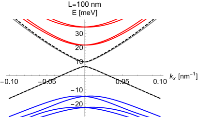
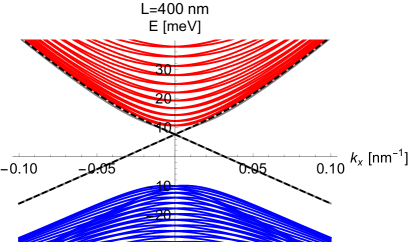
Figure 1: Bulk and edge Hamiltonian spectra for two strip sizes $L=100$ and $L=400$ nm as a function of the wavevector component $k_{x}$ for the material parameters in Table 1. Conduction states in red and valence states in blue color. The four edge states are indicated in black color (solid and dashed). The gap closes as $L$ increases.

As we already anticipated in Sec. III.1, this gap shows an exponential decay with modulations/oscillations as function of the strip width $L$, as showed in Figure 2 (red dots). We have chosen $\Delta_{z}=10$ meV this time for computational convenience, for which gap oscillations occur for smaller values of $L$ (smaller Hamiltonian matrix sizes and less computational resources are required). Sudden gap drops occur at the critical strip widths $L_{c}\simeq 100$ and $L_{c}\simeq 220$nm.

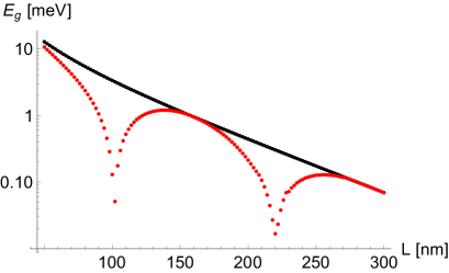
Figure 2: Energy gap (logarithmic scale) of the of edge states as a function of the strip width $L$. The gap at the $\Gamma$ point $E_{g}^{\Gamma}$ (black color) shows an exponential decay, whereas the minimum gap $E_{g}$ (red color) exhibits oscillations with sudden drops for some critical strip widths values ($L_{c}\simeq 100$ and 220 nm). This time we choose the SOC parameter $\Delta_{z}~{}=~{}10$ meV for computational convenience.

The exponential decay is captured by the gap $E_{g}^{\Gamma}=[E_{1c}(0)-E_{1v}(0)]$ at the $\Gamma$ point (black points). A fit of nine values of $E_{g}^{\Gamma}$ at $L=100,\dots,500$, in steps of $\Delta L=50$, provides the expression

$$E_{g}^{\Gamma}(L)\simeq e^{2.991-0.019L}$$ (13)

with determination coefficient $R^{2}>0.999$.

These gap oscillations have non trivial consequences in the charge conductance of the edge states given by the Landauer-Büttiker formula

$$G=\frac{1}{e^{(E_{g}/2-\mu_{F})/k_{B}T}+1}-\frac{1}{e^{(-E_{g}/2-\mu_{F})/k_{B}T}+1}+1$$ (14)

in $2e^{2}/h$ units. In Fig. 3 we plot the charge conductance as a function of the chemical potential $\mu_{F}$ and the width $L$ of the strip at temperature $T=3$ K, for the energy gaps $E_{g}$ (left panel) and $E_{g}^{\Gamma}$ (right panel). Sudden gap drops at the critical strip widths $L_{c}\simeq 100$ and $L_{c}\simeq 220$nm yield maximum charge conductance regardless the value of $\mu_{F}$. This phenomenon does not occur for $E_{g}^{\Gamma}$.

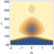
Figure 3: Variation of the conductance (in $2e^{2}/h$ units) as a function of the chemical potential $\mu_{F}$ and the width $L$ of the strip at temperature $T=3$ K. Left panel using the oscillating gap $E_{g}$ and right panel using the gap $E_{g}^{\Gamma}$ at the $\Gamma$ point (resp. red and black curves of Figure 2). Color scale varies from 0 (darkest) to 1 (brightest).

Gap drops also occur when varying the Rashba term $\xi=15.6|e\mathcal{E}_{z}|$ by applying a perpendicular electric field $\mathcal{E}_{z}$, as shown in Fig. 4. For a strip width of $L=200$ nm, the gap drops down to $E_{g}\simeq 0.01$ meV for an electric field of $|\mathcal{E}_{z}|=22.4$ mV/nm (that is, $\xi\simeq 350$meV.nm), and the charge conductance rises to $G\simeq 0.9$. As suggested by [14, 25], if it is possible to have two independent control gates, one for the SIA and other to change the Fermi energy level, then the variation of the charge conductance as function of the chemical potential ($\mu_{F}$) would be useful to design a QSH field effect transistor.

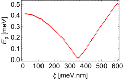
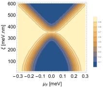
Figure 4: Left panel: energy gap $E_{g}$ as a function of the Rashba coupling term $\xi$ for $L=200$ nm. Right panel: variation of the conductance (in $2e^{2}/h$ units) as a function of the chemical potential $\mu_{F}$ and $\xi$ for $L=200$ nm and temperature $T=0.3$ K; color scale varies from 0 (darkest) to 1 (brightest).

IV Edge states localization properties

We now proceed to analyze the localization properties of the four edge states $\{\Psi_{1c},\Psi_{1v},\Psi_{2c},\Psi_{2v}\}$, both in position $y$ and momentum $k=k_{x}$ independent spaces, each one of them taking the form given in (7). Let us firstly consider probability densities

$$|\Psi(k,y)|^{2} = |\psi_{\uparrow E}(k,y)|^{2}+|\psi_{\uparrow H}(k,y)|^{2}$$ (15)

$$+ |\psi_{\downarrow E}(k,y)|^{2}+|\psi_{\downarrow H}(k,y)|^{2}.$$

and normalize them according to $\int_{0}^{L}dy|\Psi(k,y)|^{2}=1$.

In Fig. 5 we represent the probability densities $|\Psi(k,y)|^{2}$ of the four edge states as a function of $y$ for several values of the momentum $k$ (varying curve thickness). They turn out to be symmetric in $k$, that is, $|\Psi_{c,v}(k,y)|^{2}=|\Psi_{c,v}(-k,y)|^{2}$, so that we take $k\in[0,\pi/a)$ for these plots. Valence band states are more localized at the boundaries $y=0,L$ than conduction band states (approximately by a factor of four times). Maximum localization at the edges for valence states occurs at $k\simeq\pm 0.21\,\mathrm{nm}^{-1}$ (see also later in Fig. 7), while for conduction states it occurs at $k=0$.

A separated study of the four probability density components (7) of the 4-spinor is shown in Fig. 6. Note that, although $|\Psi_{c,v}(k,y)|^{2}$ does not depend on the sign of $k$, each component of $\Psi$ does. Spin down valence and spin up conduction component states are localized at $y=L$ for $k<0$ and at $y=0$ for $k>0$, whereas spin up valence and spin down conduction component states are localized at $y=0$ for $k>0$ and at $y=L$ for $k<0$. Therefore, there is a symmetry in $\mathrm{sign}(ks)$ (the helicity, with $s=\pm 1$), which is a reflect of the already known spin polarization of the QSH edge states, experimentally observed in [11]. For $k=0$, the probability density components show a more balanced behavior in position space.

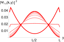
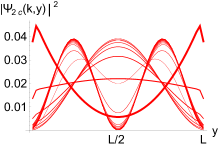
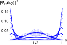
Figure 5: Probability density $|\Psi_{c,v}(k,y)|^{2}$ of the four 4-spinor edge states $\{\Psi_{1c},\Psi_{1v},\Psi_{2c},\Psi_{2v}\}$ (conduction -red- and valence -blue-) in position ($y$) space for $L=100$ nm and momentum $k\in[0,\pi/a)$ (symmetric in $k$). The thickness of the probability density curves decreases with $k$, the thickest one corresponding to $k=0$. The maximum localization at the edges corresponds to: $k\simeq\pm 0.21\,\mathrm{nm}^{-1}$ for valence band (blue) and $k=0$ for conduction band (red).

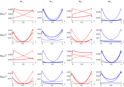
Figure 6: Component-wise probability densities of the four edge states $\{\Psi_{1c},\Psi_{1v},\Psi_{2c},\Psi_{2v}\}$, as a function of $y\in[0,L]$ ($L=100$nm), for three values of the momenta: $k_{x}=-0.005\,\mathrm{nm}^{-1}$ (dashed) $k_{x}=0.005\,\mathrm{nm}^{-1}$ (dotted) and $k_{x}=0\,\mathrm{nm}^{-1}$ (solid). Conduction in red and valence in blue colors.

Another useful measure of localization, used in multiple contexts, is the inverse participation ratio (IPR). It measures the spreading of the expansion of a normalized vector $|\psi\rangle=\sum_{n=1}^{N}p_{n}|n\rangle$ in a given basis $\{|n\rangle,n=1,\dots,N\}$. It is defined as $\mathrm{IPR}_{\psi}=\sum_{n=1}^{N}|p_{n}|^{4}$, so that $\mathrm{IPR}_{\psi}=1/N$ for an equally weighted superposition $|p_{n}|=1/\sqrt{N}$ and $\mathrm{IPR}_{\psi}=1$ for $p_{n}=\delta_{n,n_{0}}$. For the case of a free particle in a box $y\in[0,L]$, the wave function $\psi_{m}(y)=\sqrt{2/L}\sin(m\pi y/L)$, normalized according to $\int_{0}^{L}dy|\psi_{m}(y)|^{2}=1$, has an $\mathrm{IPR}=\int_{0}^{L}dy|\psi_{m}(y)|^{4}=3/(2L)$, which is the lowest expected value of the IPR in our problem. For example, for a strip width of $L=100$ nm, we have $\mathrm{IPR}=0.015$.

A measure of the spreading of a 4-spinor in position space for each value of the momentum $k$ is given by

$$\mathrm{IPR}_{\Psi}(k)=\int_{0}^{L}dy|\Psi(k,y)|^{4},$$ (16)

where now we understand

$$|\Psi|^{4}=|\psi_{\uparrow E}|^{4}+|\psi_{\uparrow H}|^{4}+|\psi_{\downarrow E}|^{4}+|\psi_{\downarrow H}|^{4}.$$ (17)

Fig. 7 displays $\mathrm{IPR}_{\Psi}(k)$ for the four edge states. Both valence edge states, $\Psi_{1v}$ and $\Psi_{2v}$, show maximum localization in position space at $k\simeq\pm 0.21\,\mathrm{nm}^{-1}$ (mentioned above) while conduction states are more delocalized in space for all values of $k\in(-\pi/a,\pi/a)$.

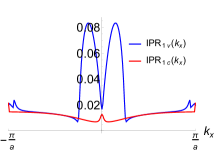
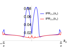
Figure 7: Localization of conduction (red) and valence (blue) edge states in position space for each value of the momentum ($k_{x}$) as measured by the inverse participation ratio (IPR) for a strip width of $L=100$ nm. $\mathrm{IPR}_{v}(k)$ is maximum at $k\simeq\pm 0.21\,\mathrm{nm}^{-1}$ for which edge states are maximally localized on the boundaries $y=0,L$

Finally, we analyze the spreading of the expansion of edge states in momentum space $k$ for a given position $y$. To do that, now we have to normalize 4-spinors as $\int_{-\pi/a}^{\pi/a}dk|\Psi(k,y)|^{2}=1$ and define

$$\mathrm{IPR}_{\Psi}(y)=\int_{-\pi/a}^{\pi/a}dk|\Psi(k,y)|^{4}.$$ (18)

Fig. 8 shows that edge states participate of less momenta at $y=0,L$ (higher IPR), since momentum is localized around $k=\pm 0.21\,\mathrm{nm}^{-1}$, as it was mentioned before. In the case of conduction $\Psi_{2c}$ and valence $\Psi_{2v}$, the corresponding edge states also participate of less momenta (higher IPR) at the center of the strip $y=L/2$.

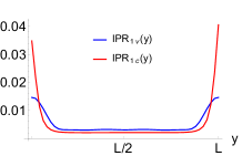
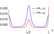
Figure 8: Localization of conduction (red) and valence (blue) edge states in momentum space for each value of the position ($y$) as measured by the inverse participation ratio (IPR) for a strip width of $L=100$ nm. Edge states participate of less momenta at $y=0,L$. $\Psi_{2c}$ and $\Psi_{2v}$ also show higher IPR (momentum localization) at the center of the strip $y=L/2$.

The IPR concept is related to the purity of a density matrix, which measures the degree of entanglement of a given physical state. In the next section we study entanglement properties of our edge states.

V Spin probabilities and spin-band entanglement measures

In order to compute quantum correlations in our system, we shall use two different entanglement measures.

V.1 Reduced density matrix, spin probabilities and linear entropy

Let $\rho=|\Psi\rangle\langle\Psi|$ the $4\times 4$ density matrix $\rho$ corresponding to a normalized 4-spinor state (7). Denoting the 4-spinor $\Psi(k,y)$ column 4-vector as a function of position $y$ and momentum $k$, the $4\times 4$ density matrix at $(k,y)$ acquires the form

$$\rho(k,y)=\frac{\Psi(k,y)\Psi^{\dagger}(k,y)}{\Psi^{\dagger}(k,y)\Psi(k,y)},$$ (19)

where we are normalizing by the scalar quantity $\Psi^{\dagger}(k,y)\Psi(k,y)=|\Psi(k,y)|^{2}$ in (15) in order to have $\mathrm{tr}(\rho(k,y))=1$ at each point $(k,y)$. The 16 density matrix entries $\rho_{ij},i,j=1,2,3,4$ are referenced to the basis

$$|1\rangle = |\uparrow\rangle\otimes|E\rangle,\quad|2\rangle=|\uparrow\rangle\otimes|H\rangle,$$

$$|3\rangle = |\downarrow\rangle\otimes|E\rangle,\quad|4\rangle=|\downarrow\rangle\otimes|H\rangle.$$ (20)

The reduced density matrix (RDM) $\varrho$ to the spin subsystem is obtained by taking the partial trace

$$\varrho=\mathrm{tr}_{EH}(\rho)=\left(\begin{array}[]{cc}\rho_{11}+\rho_{22}&\rho_{13}+\rho_{24}\\ \rho_{31}+\rho_{42}&\rho_{33}+\rho_{44}\\ \end{array}\right).$$ (21)

The diagonal components of the RDM

$$\varrho_{11}=\rho_{11}+\rho_{22}=P_{\Psi}(\uparrow),\quad\varrho_{22}=\rho_{33}+\rho_{44}=P_{\Psi}(\downarrow),$$ (22)

represent the probabilities of finding the electron with spin up or down, respectively, whereas the modulus of the off-diagonal elements

$$|\varrho_{12}|=|\varrho_{21}|=|\rho_{13}+\rho_{24}|=P_{\Psi}(\uparrow\to\downarrow),$$ (23)

represent the spin transfer probability amplitudes (also called coherences in quantum information jargon).

In Fig. 9 we plot the probabilities $P_{\Psi}(\uparrow)$ and $P_{\Psi}(\downarrow)$ for the first conduction $\Psi_{1c}$ and valence $\Psi_{1v}$ edge states as a function of $(k,y)$. Lighter colors represent higher probability zones. Probability densities are unbalanced at the boundaries $y=0,L$ depending on the propagation direction given by the sign of $k$. This is a reflection of the existence of counterpropagating modes of opposite spin at the edges. Note that these probabilities are invariant under the sign of the helicity $\mathrm{sign}(ks)$, with $s=\pm 1$ the spin, for each value of $y$. This is again a reflect of the experimental confirmation in [11] that the transport in the edge channels is spin polarized.

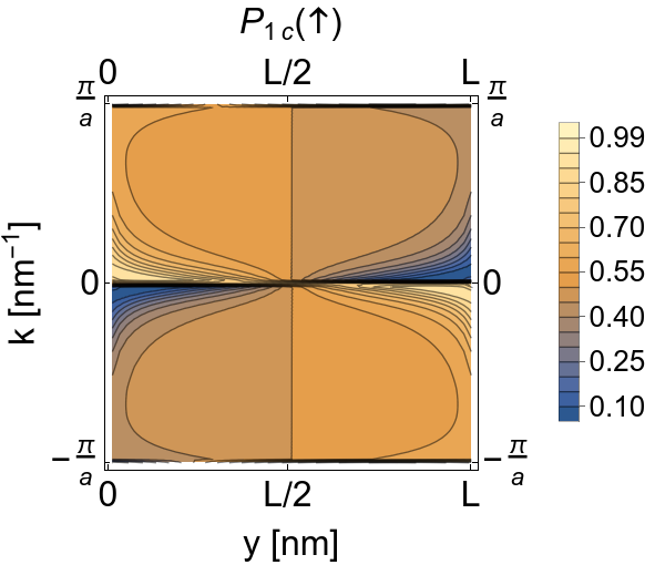
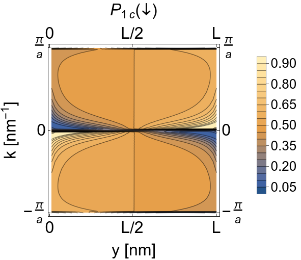
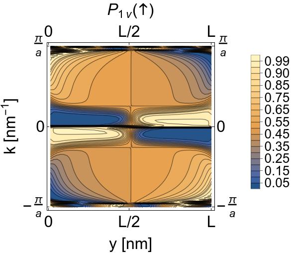
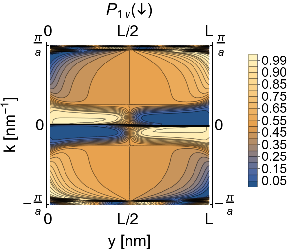
Figure 9: Probabilities to find the electron with spin $\uparrow$ and down $\downarrow$ for the first conduction $\Psi_{1c}$ and valence $\Psi_{1v}$ edge states as a function of momentum $k\in(-\pi/a,\pi/a)$ and position $y\in(0,L)$ for a strip width of $L=100$ nm. Lighter zones correspond to higher probability.

In Fig. 10 we plot spin transfer probability amplitudes for $\Psi_{1c}$ and $\Psi_{1v}$ as a function of $k$ and $y$ for a strip width of $L=100$ nm. The maximum probability $P_{1c}^{\mathrm{max.}}(\uparrow\to\downarrow)\simeq 1/2$ is attained at the center of the strip $y=L/2$ for $k\simeq\pm 1.54\,\mathrm{nm}^{-1}$, and the minimum probability $P_{1c}^{\mathrm{min.}}(\uparrow\to\downarrow)=0.003$ is attained at $y=34$ and $y=66$ nm for $k\simeq\pm 0.1\,\mathrm{nm}^{-1}$. These extrema are quite flat, as can be perceived in Fig. 10. Analogously, for the first valence edge state, there is a quite flat zone of maximum probability $P_{1v}^{\mathrm{max.}}(\uparrow\to\downarrow)\simeq 1/2$ around $y=L/2$ and $k\simeq\pm 1.4\,\mathrm{nm}^{-1}$, and of minimum probability $P_{1v}^{\mathrm{min.}}(\uparrow\to\downarrow)=0.02$ around $y=22$ and $y=78$ nm for $k\simeq\pm 0.1\,\mathrm{nm}^{-1}$.

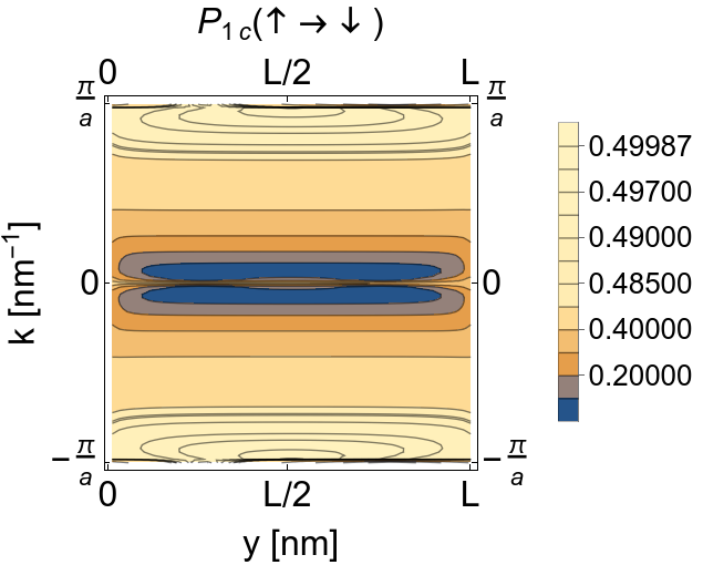
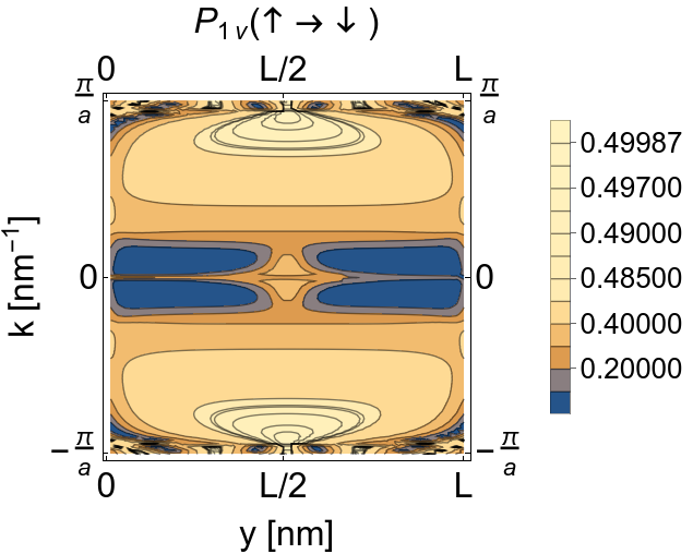
Figure 10: Spin transfer probability amplitudes for first conduction $\Psi_{1c}$ and valence $\Psi_{1v}$ edge states as a function of momentum $k\in(-\pi/a,\pi/a)$ and position $y\in(0,L)$ for a strip width of $L=100$ nm. Lighter zones correspond to higher probability amplitudes.

We now analyze the spin-band quantum correlations by means of the linear entropy, which is defined through the purity $\mathrm{tr}(\varrho^{2})$ as

$$S=1-\mathrm{tr}(\varrho^{2}).$$ (24)

Maximum entanglement means $S_{\mathrm{max}}=1/2$ for a $2\times 2$ RDM $\varrho$, whereas pure states have $S=0$.

In Fig. 11 we show the linear entropies $S_{i}(k,y)$ of the four edge states $\Psi_{i}$, with $i\in\{1c,1v,2c,2v\}$, as a function of $(k,y)$ for a strip width of $L=100$ nm. The entropy is symmetric in $k$ and $y$, and we shall only show half of the interval in momentum space (that is $k\in(0,\pi/a)$). For $\Psi_{1c}$ and $\Psi_{2c}$, the maximum entanglement $S\simeq 1/2$ occurs at $y=L/2$ and $k\simeq 0.11\,\mathrm{nm}^{-1}$. For $\Psi_{1v}$, the maximum entanglement $S\simeq 0.38$ occurs at $y=L/2$ and $k\simeq 0.3\,\mathrm{nm}^{-1}$. For $\Psi_{1v}$, the maximum entanglement $S\simeq 0.38$ occurs at $y=L/2$ and $k\simeq 0.3\,\mathrm{nm}^{-1}$ whereas for $\Psi_{2v}$, the maximum entanglement $S\simeq 0.33$ occurs at $y\simeq 32$ and $y\simeq 68$ nm and $k\simeq 0.36\,\mathrm{nm}^{-1}$.

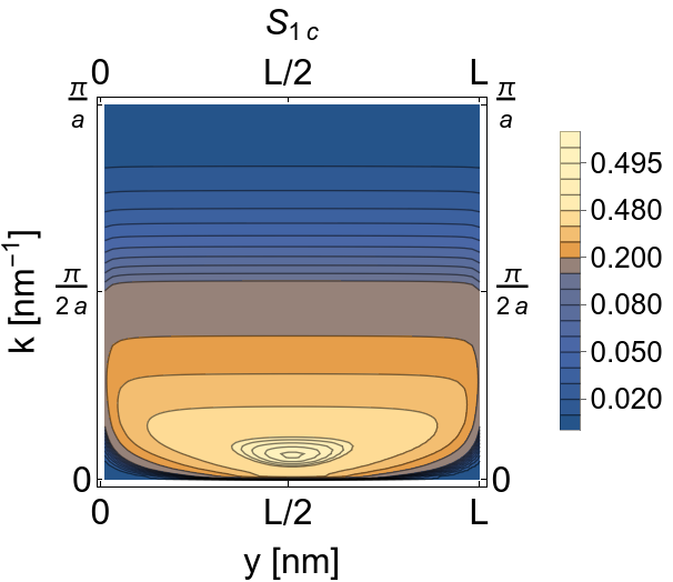
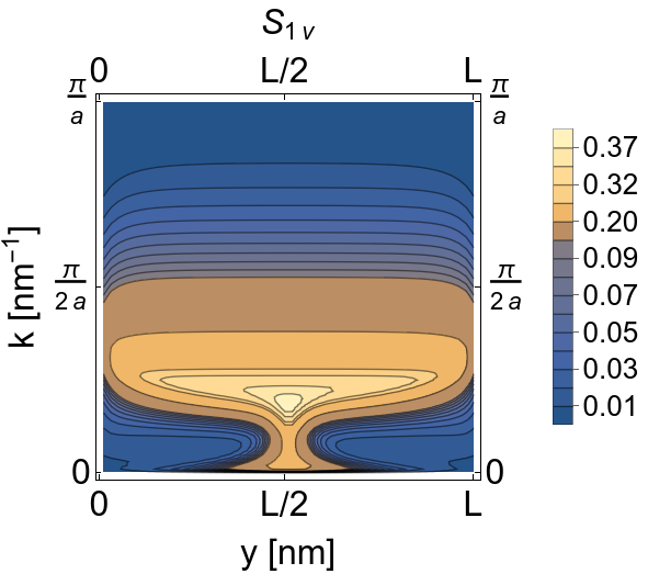
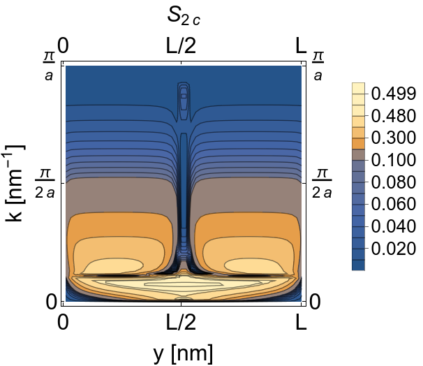
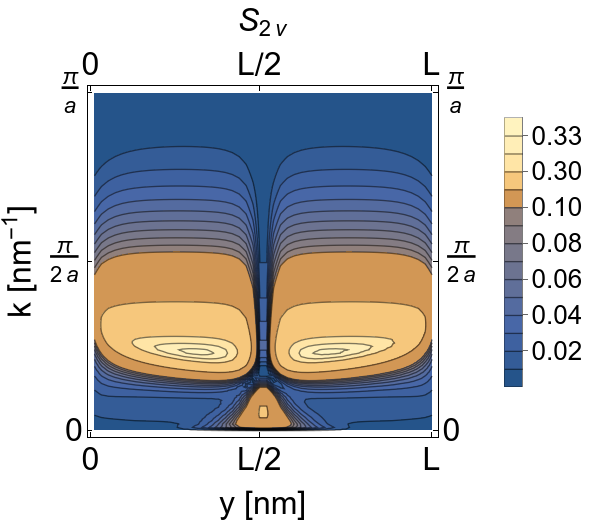
Figure 11: Linear entropy for spin-band correlations of the four edge states $\Psi_{i},i\in\{1c,1v,2c,2v\}$ as a function of momentum $k\in(0,\pi/a)$ ($S$ is symmetric in $k$ and $y$) and position $y\in(0,L)$ for a strip width of $L=100$ nm. Lighter zones correspond to higher entropy.

V.2 Schlienz & Mahler entanglement measure

We shall also briefly discuss other related entanglement measure in the field of quantum information, like the one proposed by Schlienz & Mahler [35] related to a bipartite system of an arbitrary number $D$ levels (“quDits”). In our case, $D=2$ and a qubit-qubit system will make reference to spin up-down and band E-H sectors. The entanglement measure is defined as follows. The $4\times 4$ density matrix $\rho$ is now written in terms of the 16 generators of the unitary group U(4), which can be written as tensor products of Pauli matrices like in (II) and (5). More precisely

$$\rho = \frac{1}{4}\sigma_{0}\otimes\sigma_{0}+\frac{1}{4}\sum_{k=1}^{3}(\lambda^{(1)}_{k}\sigma_{k}\otimes\sigma_{0}+\lambda^{(2)}_{k}\sigma_{0}\otimes\sigma_{k})$$ (25)

$$+\frac{1}{4}\sum_{k,j}C^{(1,2)}_{kj}\sigma_{k}\otimes\sigma_{j}\,,$$

with

$$\bm{\lambda}^{(1)}=\mathrm{tr}(\rho\,\bm{\sigma}\otimes\sigma_{0}),\,\bm{\lambda}^{(2)}=\mathrm{tr}(\rho\,\sigma_{0}\otimes\bm{\sigma}),$$

$${C}^{(1,2)}_{kj}=\mathrm{tr}(\rho\,{\sigma}_{k}\otimes{\sigma}_{j}).$$ (26)

The vectors $\bm{\lambda}^{(1)}$ and $\bm{\lambda}^{(2)}$ denote the Bloch coherence vectors of the first qubit (spin up-down) and the second qubit (band E-H) and the $3\times 3$ matrix ${C}^{(1,2)}$ accounts for qubit-qubit (spin-band) correlations. The RDM on the spin sector is

$$\rho^{(1)}=\mathrm{tr}_{2}(\rho)=\frac{1}{2}\sigma_{0}+\frac{1}{2}\sum_{k=1}^{3}\lambda^{(1)}_{k}\sigma_{k}\otimes\sigma_{0},$$ (27)

and analogously on the band sector $\rho^{(2)}$. Comparing $\rho$ with the direct product $\rho^{(1)}\otimes\rho^{(2)}$, the difference comes from a $3\times 3$ entanglement matrix $M$ with components

$${M}_{jk}={C}^{(1,2)}_{jk}-\lambda^{(1)}_{j}\lambda^{(2)}_{k},\;j,k=1,2,3.$$ (28)

Based on $M$, Ref. [35] introduces a measure of “qubit-qubit” (spin-band) entanglemet given by the parameter

$$B_{\Psi}=\frac{1}{3}\mathrm{tr}({M}^{T}{M}).$$ (29)

The parameter $B$ is bounded by $0\leq B\leq 1$ and carries information about spin up and down correlations. The results for $B$ provide an equivalent behavior to the linear entropy in Figure 11, except for a scaling factor.

VI Conclusions

We have used QI theory concepts like IPR, RDM and entanglement entropies, as an interesting “microscope” to reveal details of the internal structure of HgTe QW edge states with SOC (induced by the bulk and structural inversion asymmetries) in a finite strip geometry of width $L$. To do this, we have considered a four band Hamiltonian describing the low energy effective theory. Quantitative information on the edge states energies and wavefunctions is extracted from a numerical Hamiltonian diagonalization approach, which is complemented by an analytic (more qualitative) view. We corroborate previous results on the intriguing oscillatory dependence of the energy gap with $L$, this time for a more general SOC, with sudden gap drops for critical strip widths $L_{c}$. The non-trivial consequences of the Rashba term on the charge conductance are also reviewed, with a possible design of a QSH FET.

The spin polarization structure of edge states in position $y\in[0,L]$ and momentum $k_{x}\in(-\pi/a,\pi/a)$ has also been evidenced by using probability density and IPR plots. The IPR analysis reveals that, in general, edge state wave packets participate of less and less momenta as we approach the boundaries $y=0,L$ of the strip, with maximum localization for certain values of the momenta $\pm k_{x}$ in the vicinity of the $\Gamma$ point.

Complementary information on the structure of spin polarization of edge states in $(k_{x},y)$ space is extracted from the RDM for the spin subsystem. Contour plots of the RDM entries show the extremal values of spin up and down and spin transfer probabilities in $(k_{x},y)$ space. Also, entropies of the RDM inform on regions in $(k_{x},y)$ space where the spin sector is highly entangled with the rest of the system, due to spin-orbit coupling. The behavior of the quantum correlations does not seem to depend on the particular entanglement measure used.

References

- Sinova et al. [2015] J. Sinova, S. O. Valenzuela, J. Wunderlich, C. H. Back, and T. Jungwirth, Spin hall effects, Rev. Mod. Phys. 87, 1213 (2015).
- Nagaosa et al. [2010] N. Nagaosa, J. Sinova, S. Onoda, A. H. MacDonald, and N. P. Ong, Anomalous hall effect, Rev. Mod. Phys. 82, 1539 (2010).
- Maciejko et al. [2011] J. Maciejko, T. L. Hughes, and S.-C. Zhang, The quantum spin hall effect, Annual Review of Condensed Matter Physics 2, 31 (2011).
- Haldane [1988] F. D. M. Haldane, Model for a quantum hall effect without landau levels: Condensed-matter realization of the "parity anomaly", Phys. Rev. Lett. 61, 2015 (1988).
- Gusynin and Sharapov [2005] V. P. Gusynin and S. G. Sharapov, Unconventional integer quantum hall effect in graphene, Phys. Rev. Lett. 95, 146801 (2005).
- Kane and Mele [2005a] C. L. Kane and E. J. Mele, Quantum spin Hall effect in graphene, Phys. Rev. Lett. 95, 226801 (2005a).
- Bernevig et al. [2006] B. A. Bernevig, T. L. Hughes, and S.-C. Zhang, Quantum spin Hall effect and topological phase transition in HgTe quantum wells, Science 314, 1757 (2006).
- Bernevig and Zhang [2006] B. A. Bernevig and S.-C. Zhang, Quantum spin hall effect, Phys. Rev. Lett. 96, 106802 (2006).
- König et al. [2007] M. König, S. Wiedmann, C. Brüne, A. Roth, H. Buhmann, L. W. Molenkamp, X.-L. Qi, and S.-C. Zhang, Quantum spin hall insulator state in hgte quantum wells, Science 318, 766 (2007).
- Dai et al. [2008] X. Dai, T. L. Hughes, X.-L. Qi, Z. Fang, and S.-C. Zhang, Helical edge and surface states in hgte quantum wells and bulk insulators, Phys. Rev. B 77, 125319 (2008).
- Brüne et al. [2012] C. Brüne, A. Roth, H. Buhmann, E. M. Hankiewicz, L. W. Molenkamp, J. Maciejko, X.-L. Qi, and S.-C. Zhang, Spin polarization of the quantum spin hall edge states, Nature Physics 8, 485 (2012).
- Yang et al. [2008] W. Yang, K. Chang, and S.-C. Zhang, Intrinsic spin hall effect induced by quantum phase transition in hgcdte quantum wells, Phys. Rev. Lett. 100, 056602 (2008).
- Zhang et al. [2021] T.-Y. Zhang, Q. Yan, and Q.-F. Sun, Constructing low-dimensional quantum devices based on the surface state of topological insulators, Chinese Physics Letters 38, 077303 (2021).
- Liu et al. [2008] C. Liu, T. L. Hughes, X.-L. Qi, K. Wang, and S.-C. Zhang, Quantum spin hall effect in inverted type-ii semiconductors, Phys. Rev. Lett. 100, 236601 (2008).
- Shen [2012] S.-Q. Shen, Topological Insulators: Dirac Equation in Condensed Matters (Springer-Verlag Berlin Heidelberg, 2012).
- Bernevig [2013] B. A. Bernevig, Topological Insulators and Topological Superconductors (Princeton University Press, 2013).
- J. K. Asboth and A. Palyi [2016] L. O. J. K. Asboth and A. S. A. Palyi, A Short Course on Topological Insulators: Band Structure and Edge States in One and Two Dimensions (Springer International Publishing Switzerland, 2016).
- Hasan and Kane [2010] M. Z. Hasan and C. L. Kane, Colloquium: Topological insulators, Rev. Mod. Phys. 82, 3045 (2010).
- Qi and Zhang [2011] X.-L. Qi and S.-C. Zhang, Topological insulators and superconductors, Rev. Mod. Phys. 83, 1057 (2011).
- Hsieh et al. [2008] D. Hsieh, D. Qian, L. Wray, Y. Xia, Y. S. Hor, R. J. Cava, and M. Z. Hasan, A topological dirac insulator in a quantum spin hall phase, Nature 452, 970 (2008).
- Hsieh et al. [2009] D. Hsieh, Y. Xia, L. Wray, D. Qian, A. Pal, J. H. Dil, J. Osterwalder, F. Meier, G. Bihlmayer, C. L. Kane, Y. S. Hor, R. J. Cava, and M. Z. Hasan, Observation of unconventional quantum spin textures in topological insulators, Science 323, 919 (2009).
- Shan et al. [2010] W.-Y. Shan, H.-Z. Lu, and S.-Q. Shen, Effective continuous model for surface states and thin films of three-dimensional topological insulators, New Journal of Physics 12, 043048 (2010).
- Qi et al. [2006] X.-L. Qi, Y.-S. Wu, and S.-C. Zhang, Topological quantization of the spin hall effect in two-dimensional paramagnetic semiconductors, Phys. Rev. B 74, 085308 (2006).
- König et al. [2008] M. König, H. Buhmann, L. W. Molenkamp, T. Hughes, C.-X. Liu, X.-L. Qi, and S.-C. Zhang, The quantum spin Hall effect: Theory and experiment, Journal of the Physical Society of Japan 77, 031007 (2008).
- Zhi and Bin [2014] C. Zhi and Z. Bin, Finite size effects on helical edge states in hgte quantum wells with the spin—orbit coupling due to bulk- and structure-inversion asymmetries, Chinese Physics B 23, 037304 (2014).
- Zhou et al. [2008] B. Zhou, H.-Z. Lu, R.-L. Chu, S.-Q. Shen, and Q. Niu, Finite size effects on helical edge states in a quantum spin-hall system, Phys. Rev. Lett. 101, 246807 (2008).
- Jiang et al. [2012] H.-C. Jiang, Z. Wang, and L. Balents, Identifying topological order by entanglement entropy, Nature Physics 8, 902 (2012).
- Zeng et al. [2019] B. Zeng, X. Chen, D.-L. Zhou, and X.-G. Wen, Quantum Information Meets Quantum Matter: From Quantum Entanglement to Topological Phases of Many-Body Systems (Springer Nature, 2019).
- Calixto et al. [2022] M. Calixto, N. A. Cordero, E. Romera, and O. Castaños, Signatures of topological phase transitions in higher Landau levels of HgTe/CdTe quantum wells from an information theory perspective, Physica A: Statistical Mechanics and its Applications 605, 128057 (2022).
- Calixto and Romera [2015] M. Calixto and E. Romera, Inverse participation ratio and localization in topological insulator phase transitions, Journal of Statistical Mechanics: Theory and Experiment 2015, P06029 (2015).
- Novik et al. [2005] E. G. Novik, A. Pfeuffer-Jeschke, T. Jungwirth, V. Latussek, C. R. Becker, G. Landwehr, H. Buhmann, and L. W. Molenkamp, Band structure of semimagnetic quantum wells, Phys. Rev. B 72, 035321 (2005).
- Franz and [Eds.] M. Franz and L. M. (Eds.), Topological Insulators, Contemporary Concepts of Condensed Matter Science, Vol. 6 (Elsevier, Amsterdam, The Netherlands, 2013).
- Kane and Mele [2005b] C. L. Kane and E. J. Mele, topological order and the quantum spin hall effect, Phys. Rev. Lett. 95, 146802 (2005b).
- Rothe et al. [2010] D. G. Rothe, R. W. Reinthaler, C.-X. Liu, L. W. Molenkamp, S.-C. Zhang, and E. M. Hankiewicz, Fingerprint of different spin-orbit terms for spin transport in hgte quantum wells, New Journal of Physics 12, 065012 (2010).
- Schlienz and Mahler [1995] J. Schlienz and G. Mahler, Description of entanglement, Phys. Rev. A 52, 4396 (1995).