Estimating Reaction Barriers
with Deep Reinforcement Learning

Abstract

Stable states in complex systems correspond to local minima on the associated potential energy surface. Transitions between these local minima govern the dynamics of such systems. Precisely determining the transition pathways in complex and high-dimensional systems is challenging because these transitions are rare events, and isolating the relevant species in experiments is difficult. Most of the time, the system remains near a local minimum, with rare, large fluctuations leading to transitions between minima. The probability of such transitions decreases exponentially with the height of the energy barrier, making the system’s dynamics highly sensitive to the calculated energy barriers. This work aims to formulate the problem of finding the minimum energy barrier between two stable states in the system’s state space as a cost-minimization problem. We propose solving this problem using reinforcement learning algorithms. The exploratory nature of reinforcement learning agents enables efficient sampling and determination of the minimum energy barrier for transitions.

1 Introduction

There are multiple sequential decision-making processes one comes across in the world, such as control of robots, autonomous driving, and so on. Instead of constructing an algorithm from the bottom up for an agent to solve these tasks, it would be much easier if we could specify the environment and the state in which the task is considered solved, and let the agent learn a policy that solves the task. Reinforcement learning attempts to address this problem. It is a hands-off approach that provides a feature vector representing the environment and a reward for the actions the agent takes. The objective of the agent is to learn the sequence of steps that maximizes the sum of returns.

One widespread example of a sequential decision-making process where reinforcement learning is utilized is solving mazes Mannucci and van Kampen [2016]. The agent, a maze runner, selects a sequence of actions that might have long-term consequences. Since the consequences of immediate actions might be delayed, the agent must evaluate the actions it chooses and learn to select actions that solve the maze. Particularly, in the case of mazes, it might be relevant to sacrifice immediate rewards for possibly larger rewards in the long term. This is the exploitation-exploration trade-off, where the agent has to learn to choose between leveraging its current knowledge to maximize its current gains or further increasing its knowledge for some possibly larger reward in the long term, possibly at the expense of short-term rewards. The process of learning by an agent while solving a maze is illustrated in Figure 1.

(a)

(b)

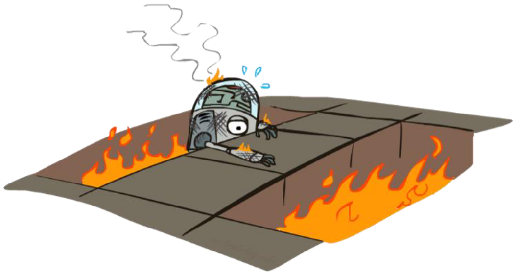
(c)

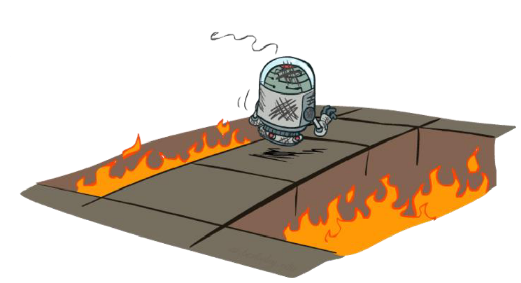
(d)

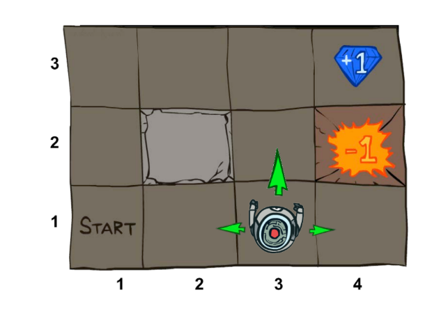
(e)

(f)

Figure 1: Maze solving using reinforcement learning: (a) The agent is at a state at a particular time step. (b) The agent takes an action (according to the policy it is supposed to learn) and reaches the next state. (c) The agent records the reward obtained by taking the action at that state. (d) The agent takes another action to explore the environment. In most reinforcement learning algorithms this (state, action, reward, next state, next action) tuple is stored while the agent is learning. With a large number of interactions with the environment (e), where the agent takes an action at a state to learn the reward obtained, the agent learns a policy (f) which maximizes the rewards collected by the agent. The policy (f) gives the sequence of actions that the agent has to take from the initial state to the final state so that it collects the maximum rewards in the episode.

GridWorld is an environment for reinforcement learning that mimics a maze Sutton and Barto [1998]. The agent is placed at the start position in a maze with blocked cells, and the agent tries to reach a stop position with the minimum number of steps possible. One might note an analogy of a maze runner with an agent negotiating the potential energy landscape of a transition event for a system along the saddle point with the minimum height. The start state and the stop state are energy minima on the potential energy surface, separated by an energy barrier for the transition. The agent would have to perform a series of perturbations to the system to take it from one minimum (the start state) to another (the end state) through the located saddle point. As in the maze-solving problem, the agent tries to identify the pathway with the minimum energy barrier. If the number of steps is considered the cost incurred in a normal maze, it is the energy along the pathway that is the cost for the transition event. A comparison is attempted in Figure 2.

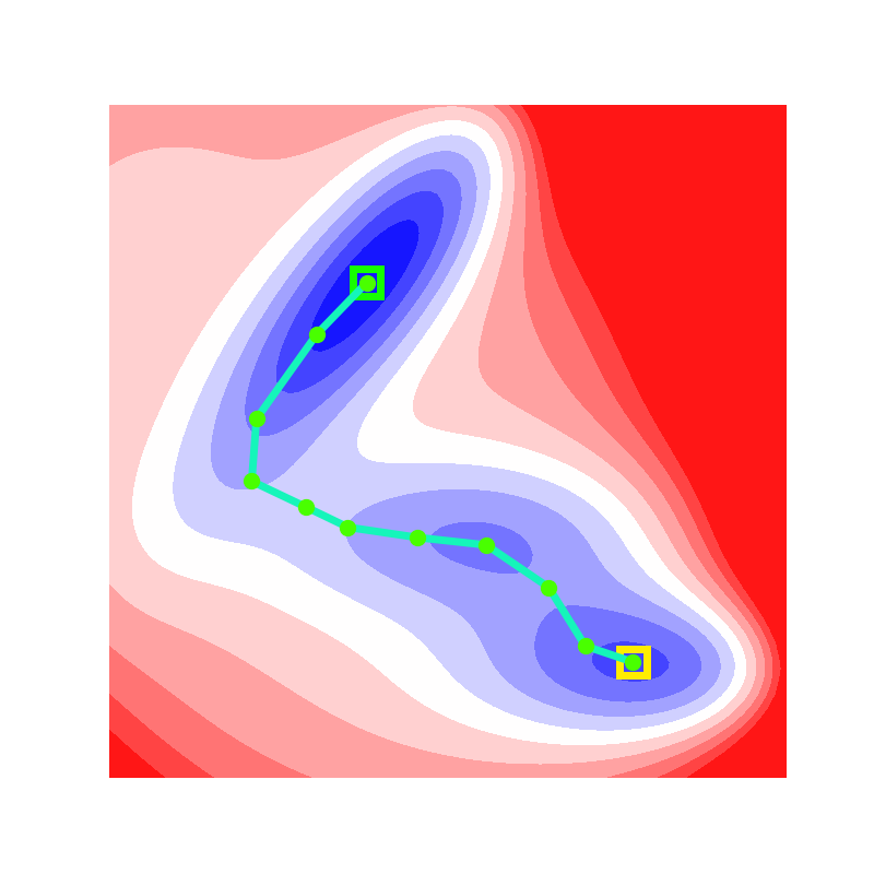
(a)

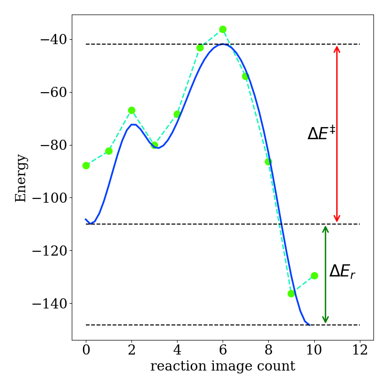
(b)

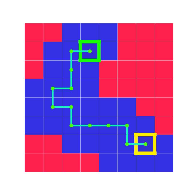
(c)

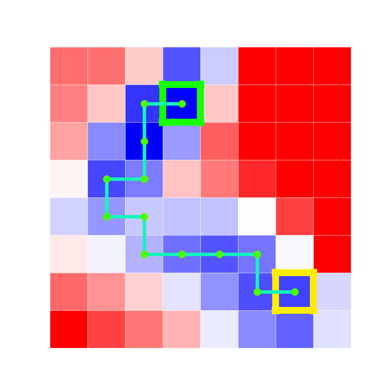
(d)

Figure 2: Estimating reaction barriers by modeling the potential energy surface as a maze: (a) The pathway with the lowest energy barrier as determined by a growing string method on the potential energy surface with 9 intermediate images. (b) The reaction profile, plotted as a solid blue line (interpolated to give a smooth curve) from the pathway determined by the growing string method. The reaction barrier is marked as $\Delta E^{\ddagger}$. (c) The same potential energy surface as in (a) is course grained to construct the maze. The initial state is marked as the yellow box while the final state is marked as the green box. The agent can move to the blue boxes while the red boxes represent walls. The energy cutoff $0$ is chosen to determine whether a grid box is a wall or not. (d) Instead of the extreme classification of a grid box as a wall or not, each grid box is assigned an energy value. The agent is then allowed to learn the path with the minimum sum of energies along it’s path from the initial state to the final state. The energy profile for the pathway identified by the agent in this maze is plotted as the dashed green line in (b). As it might be seen, coarse-graining the potential energy surface into a $8\times 8$ maze, ans solving then solving it using standard reinforcement learning algorithms provides a reasonable starting point to solving the problem.

The problem of locating the minimum energy barrier for a transition has applications in physical phase transitions, synthesis plans for materials, activation energies for chemical reactions, and the conformational changes in biomolecules that lead to reactions inside cells. In most of these scenarios, the dynamics are governed by the kinetics of the system (rather than the thermodynamics) because the thermal energy of the system is much smaller than the energy barrier of the transition. This leads to the system spending most of its time around the minima, and some random large fluctuations in the system lead to a transition. This is precisely why transition events are rare and difficult to isolate and characterize with experimental methods. Moreover, these ultra-fast techniques can be applied to only a limited number of systems. Because transition events are rare, sampling them using Monte Carlo methods requires long simulation times, making them inefficient Bolhuis and Swenson [2021]. To sample the regions of the potential energy surface around the saddle point adequately, a large number of samples have to be drawn. Previous work has been done to identify the saddle point and determine the height of the transition barrier—transition path sampling Jung et al. [2023], nudged elastic band Henkelman et al. [2000], growing string method Jafari and Zimmerman [2017], to name a few—which use ideas from gradient descent. However, even for comparatively simple reactions, these methods are not always guaranteed to find the path with the energy barrier that is a global minimum because the initial guess for the pathway might be wrong and lead to a local minimum.

With the advent of deep learning and the use of neural nets as function approximators for complex mappings, there has been increased interest in the use of machine learning Rotskoff et al. [2022] to either guess the configuration of the saddle point along the pathway (whose energy can then be determined by standard ab initio methods) or directly determine the height of the energy barrier given the two endpoints of the transition. Graph neural networks Wander et al. [2024], generative adversarial networks Makoś et al. [2021], gated recurrent neural networks Choi [2023], transformers Luong and Singh [2024], machine-learned potentials Heinen et al. [2022], Jackson et al. [2021], and so on, have been used to optimize the pathway for such transitions.

Noting the superficial similarities between solving a maze and determining the transition pathway with the lowest energy barrier, we propose to use standard and tested deep reinforcement learning algorithms used to solve mazes in an attempt to solve the problem of finding minimum energy pathways. The problem is formulated as a min-cost optimization problem in the state space of the system. We use this formulation to determine the barrier height of the optimal pathway in the Mueller-Brown potential. Neural nets are used as the actor and critic function approximators, and a randomly perturbed policy is used to facilitate exploration of the potential energy surface by the agent. Delayed policy updates and target policy averaging are used to stabilize the learning, especially during the first few epochs, which are crucial to the optimal performance of the agent.

Section 2 describes the methods used to formulate the problem as a Markov decision process and the algorithm used to solve it. Section 3 elaborates on the experiments where the formulated method is used to determine the barrier height of a transition on the Mueller-Brown potential. Section 4 contains a short discussion of the work in the context of other similar studies and the conclusions drawn from this work.

2 Methods

To solve the problem of finding a pathway with the lowest energy barrier for a transition using reinforcement learning, one has to model it as a Markov decision process. Any Markov decision process consists of (state, action, next state) tuples. In this case, the agent starts at the initial state (a local minimum) and perturbs the system (the action) to reach a new state. Since the initial state was an energy minimum, the current state will have higher energy. However, as in many sequential control problems, the reward is delayed. A series of perturbations that lead to states with higher energies might enable the agent to climb out of the local minimum into another one containing the final state. By defining a suitable reward function and allowing the agent to explore the potential energy surface, it is expected that the agent will learn a path from the initial to the final state that maximizes the rewards. If the reward function is defined properly, it should correspond to the pathway with the lowest energy barrier for the transition.

Once the problem is formulated as a Markov decision process, it can be solved by some reinforcement learning algorithm. Twin Delayed Deep Deterministic Policy Gradient (TD3) Fujimoto et al. [2018] is a good start because it prevents the overestimation of the state value function, which often leads to the agent exploiting the errors in the value function and learning a sub-optimal policy. Soft Actor Critic (SAC) Haarnoja et al. [2018] tries to blend the deterministic policy gradient with a stochastic policy optimization, promoting exploration by the agent. In practice, using a stochastic policy to tune exploration often accelerates the agent’s learning.

2.1 Markov Decision Process

The Markov decision process is defined on:

• a state space $\mathcal{S}$, consisting of states $s\in\mathbb{R}^{d}$, where $d$ is the dimensionality of the system, chosen to be the number of degrees of freedom in the system.

• a continuous action space $\mathcal{A}$, where each action $\Delta s\in\mathbb{R}^{d}:|\left(\Delta s\right)_{i}|\leq 1$ is normalized, and the action is scaled using an appropriate scaling factor $\lambda$.

At a state $s^{(k)}$, the agent takes an action $\Delta s^{(k)}$. Since the action is considered a perturbation to the current state of the system, the next state $s^{(k+1)}$ is determined from the current state $s^{(k)}$ as $s^{(k+1)}=s^{(k)}+\lambda\cdot\Delta s^{(k)}$.

To determine the minimum energy barrier for a transition, the reward for an action taking the agent to state $s^{(k+1)}$ from state $s^{(k)}$ is chosen to be the negative of the energy of the next state, $-E\left(s^{(k+1)}\right)$. The negation makes maximizing the sum of rewards collected by the reinforcement learning agent in an episode equivalent to minimizing the sum of energies along the pathway for the transition. The reward acts as immediate feedback to the agent for taking an action in a particular state. However, what is important is the long-term reward, captured by the sum of the rewards over the entire episode, leading the agent to identify a transition pathway with a low sum of energies at all intermediate steps.

Since both the state space and action space are continuous, an actor-critic based method, specifically the soft actor-critic (SAC), is used. Additionally, since the state space is continuous, the episode is deemed to have terminated when the difference between the current state and the target state is smaller than some tolerance, $x\in\mathbb{R}^{d}:|x-x_{t}|<\delta$ for some small $\delta$. Otherwise, it would be extremely unlikely that the agent would land exactly at the coordinates of the final state after taking some action.

2.2 Algorithm

Algorithm 1 Computing minimum energy barrier using SAC in environment env

1:Initialize actor net parameters $\theta$ and critic Q-net parameters $\phi_{1}$, $\phi_{2}$

2:Hard update target Q-net parameters: $\phi_{i,\text{target}}\leftarrow\phi_{i}$ for $i=1,2$

3:Initialize replay buffer $\mathcal{R}$

4:training_step = 1

5:for step = 1 to numEpisodes do

6:     state, _ = env.reset()

7:     for t = 0 to maxSteps do

8:         let actor select an action by policy $\pi_{\theta}$

9:         perturb the action with some noise $\epsilon\sim\mathcal{N}(0,\sigma)$

$$a^{(k)}=\pi_{\theta}(s^{(k)})+\text{clip}(\epsilon,-\epsilon_{\text{lim}},\epsilon_{\text{lim}})$$

10:         execute action in the env and observe the $\left(s^{(k)},a^{(k)},r^{(k)},s^{(t+1)},\text{{ done}}\right)$ tuple

11:         push it to the replay buffer $\mathcal{R}$

12:         if training_step % agent_update == 0  then

13:              sample a minibatch $\mathcal{B}$ of $\left(s,a,r,s^{\prime},\text{{ done}}\right)$ tuples from the replay buffer $\mathcal{R}$

14:              compute targets as (where $a^{\prime}=\pi_{\theta}(\cdot|s^{\prime})+\text{clip}(\epsilon,-\epsilon_{\text{lim}},\epsilon_{\text{lim}})$)

$$y(r,s^{\prime})=r+\gamma(1-\text{{done}})\left(\min_{i=1,2}Q_{\phi_{i,\text{target}}}(s^{\prime},a^{\prime})-\alpha\log\pi_{\theta}(a^{\prime}|s^{\prime}))\right)$$

15:              update critic Q-nets parameters by one step of gradient descent with loss function (with the gradient clipped by some maximum value)

$$\frac{1}{|\mathcal{B}|}\,\,\,\nabla_{\phi_{i}}\left(\sum_{s\in\mathcal{B}}\min_{i=1,2}Q_{\phi_{i}}(s,a)-y(r,s^{\prime})\right)^{2}\text{for i = 1, 2}$$

16:              if t % update_target == 0 then

17:                  update actor net parameters by one step of gradient descent with loss function (with the gradient clipped by some maximum value)

$$\frac{1}{|\mathcal{B}|}\,\,\,\nabla_{\theta}\left(\sum_{s\in\mathcal{B}}\min_{i=1,2}Q_{\phi_{i}}(s,\pi_{\theta}(s))-\alpha\log\pi_{\theta}(a|s)\right)^{2}$$

18:                  update the entropy coefficient $\alpha$ as one step of gradient descent with loss function

$$\frac{1}{|\mathcal{B}|}\,\,\,\nabla_{\alpha}\left(\sum_{s\in\mathcal{B}}-\alpha\log\pi_{\theta}(a|s)-\alpha\log a^{\prime}\right)^{2}$$

19:                  soft update the target networks: $\phi_{i,\text{target}}\leftarrow\tau\phi_{i}+(1-\tau)\phi_{i,\text{target}}$

20:              end if

21:         end if

22:     end for

23:end for

24:return the actor net parameters $\theta$ and critic Q-net parameters $\phi_{1},\phi_{2}$.

SAC, an off-policy learning algorithm with entropy regularization, is used to solve the formulated Markov Decision process because the inherent stochasticity in its policy facilitates exploration by the agent. The algorithm learns a behavior policy $\pi_{\theta}$ and two critic Q-functions, which are neural nets with parameters $\phi_{1}$ and $\phi_{2}$ (line 1 of Algorithm 1).

The agent chooses an action $a^{(k)}\equiv\Delta s^{(k)}$ to take when at state $s^{(k)}$ following the policy $\pi_{\theta}$ (line 8). The returns from the state $s^{(k)}$ when acting according to the policy $\pi$ is the discounted sum of rewards collected from that step onwards till the end of the episode: $R_{t}=-\sum_{i=t}^{T}\gamma^{i-t},E(s^{(i)})$. The objective of the reinforcement learning agent is to determine the policy $\pi^{*}$ that maximizes the returns, $R_{t}$, for states $s\in\mathcal{S}$. This is done by defining a state-action value function, $Q(s^{(i)},a^{(i)})$, which gives an estimate of the expected returns if action $a^{(i)}$ is taken by the agent when at state $s^{(i)}$: $Q(s^{(i)},a^{(i)})=\mathbb{E}\left[R_{t}:s_{t}=s^{(i)},a_{t}=a^{(i)}\right]$. Since the objective is to maximize the sum of the returns, the action-value function can be recursively defined as

$$Q(s^{(i)},a^{(i)})=-E(s^{(i+1)})+\max_{a^{(i+1)}\in\mathcal{A}}Q(s^{(i+1)},a^{(i+1)})$$

which is implemented in line 14 of Algorithm 1.

A replay buffer with a sufficiently large capacity is employed to increase the probability that independent and identically distributed samples are used to update the actor and two critic networks. The replay buffer (in line 3) is modeled as a deque where the first samples to be enqueued (which are the oldest) are also dequeued first, once the replay buffer has reached its capacity and new samples have to be added. Since an off-policy algorithm is used, the critic net parameters are updated by sampling a mini-batch from the replay buffer at each update step (line 13). Stochastic gradient descent is used to train the actor and the two critic nets.

The entropy coefficient $\alpha$ is adjusted over the course of training to encourage the agent to explore more when required and exploit its knowledge at other times (line 18) Haarnoja et al. [2019]. However, we also borrow some elements from the TD3 algorithm Fujimoto et al. [2018] to improve the learning of the agent, namely delayed policy updates and target policy smoothing. The critic Q-nets are updated more frequently than the actor and the target Q-nets to allow the critic to learn faster and provide more precise estimates of the returns from the current state. To address the problem of instability in the learning, especially in the first few episodes while training the agent, target critic nets are used. Initially, the critic nets are duplicated (line 2) and subsequently soft updates of these target nets are carried out after an interval of a certain number of steps (line 19). This provides more precise estimates for the state-action value function while computing the returns for a particular state in line 14. To encourage the agent to explore the potential energy surface, clipped noise is added to the action chosen by the actor net (line 9). This also makes it difficult for the actor to exploit imprecise Q-net estimates during the beginning of the training. The changes to the SAC algorithm, borrowed from TD3, are highlighted in blue in the pseudocode of Algorithm 1. The parameters used in the particular implementation of the algorithm are listed in Table 1.

	Parameter	Value
$Q_{\phi}(s,a)$	network architecture	4-256-256-1
	activation for hidden layer	$relu$
	activation for output layer	none
	learning rate	$10^{-4}$
$\pi_{\theta}(s)$	network architecture	2-256-256-2
	activation for hidden layer	$relu$
	activation for output layer	none
	learning rate	$10^{-4}$
Agent	$\tau$ or Polyak averaging parameter	0.005
	$\gamma$ or discount factor	$1-10^{-2}$
	scaling factor for actions	$0.015$
	optimizer	Adam
	replay buffer $\mathcal{R}$ capacity	$10^{4}$
	minibatch size for update	$128$
	maximum steps per epoch	$500$
	number of training epochs	$1000$
SAC specific	initial $\alpha$ or entropy coefficient	$0.5$
	$\alpha$ value	variable
	learning rate for $\alpha$	$10^{-4}$
TD3 specific	target update delay interval	$8$ steps
	actor noise standard deviation	$0.4$
	actor noise clip	$1.0$

Table 1: Parameters used while training the RL agent.

3 Experiments

The proposed algorithm is applied to determine the pathway with the minimum energy barrier on the M"uller–Brown potential energy surface Müller and Brown [1979]. The M"uller–Brown potential has been used to benchmark the performance of several algorithms that determine the minimum energy pathways, such as the molecular growing string method Goodrow et al. [2009], Gaussian process regression for nudged elastic bands Koistinen et al. [2017], and accelerated molecular dynamics Vlachas et al. [2022]. Therefore, it is also used in this work to demonstrate the applicability of the proposed method. A custom Gym environment Towers et al. [2023] was created following the gymnasium interface (inheriting from the class Gym) to model the problem as a Markov Decision Process to be solved by a reinforcement learning pipeline. The values for the parameters used in Algorithm 1 are listed in Table 1.

3.1 Results

The M"uller–Brown potential is characterized by the following potential:

$$V(x,y)=\sum_{i=0}^{3}W_{i}\cdot\exp\left[a_{i}\left(x-\overline{x}_{i}\right)^{2}+b_{i}\left(x-\overline{x}_{i}\right)\left(y-\overline{y}_{i}\right)+c_{i}\left(y-\overline{y}_{i}\right)^{2}\right]$$ (1)

where $W=(-200,-100,-170,15)$, $a=(-1,-1,-6.5,0.7)$, $b=(0,0,11,0.6)$, $c=(-10,-10,-6.5,0.7)$, $\overline{x}=(1,0,-0.5,-1)$, and $\overline{y}=(0,0.5,1.5,1)$. The potential energy surface for the system is plotted in Figure 3(a), and the local minima are at $(-0.558,1.442)$, $(0.623,0.028)$, and $(-0.050,0.467)$ with the value of $V(x,y)$ being $-146.7$, $-108.2$, and $-80.8$, respectively. The RL agent was trained to locate a path on this surface from $(0.623,0.028)$ with a random step (with zero mean and a standard deviation of $0.1$) added to it as the initial state to $(-0.558,1.442)$ as the terminal state, with the minimum energy barrier. The first random step was chosen to avoid the same starting point in each training iteration of the agent, so it learns a more generalized policy. Some of the parameters for the Markov Decision Process to model this potential are given in Table 2.

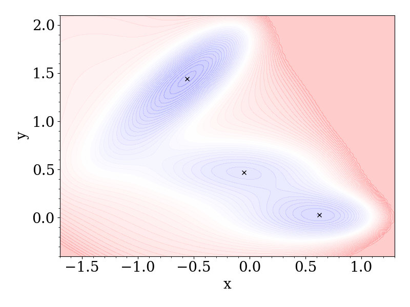
(a) Potential energy surface to find the paths with minimum energy barrier.

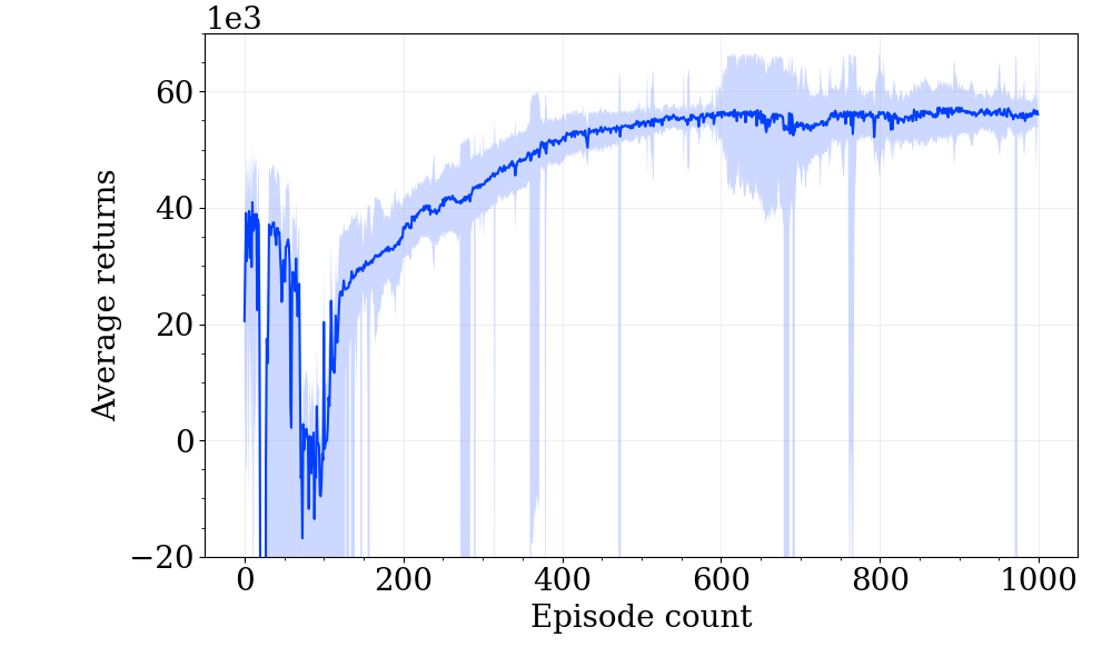
(b) Learning curve with the shaded region representing one standard deviation from the mean over $11$ trials.

Figure 3: (Left) Environment in which the agent learns to find the path with the minimum energy barrier. (right) The rising learning curve against the number of evaluation episodes indicates that the agent learns to find the path with minimum energy barrier (recall that the reward was defined as the negative of the energy of a state, which leads to ascending learning curve and maximizing of the reward indicating that the agent learning a path with lower energy barrier). The agent was run in evaluation mode once every $10$ training steps.

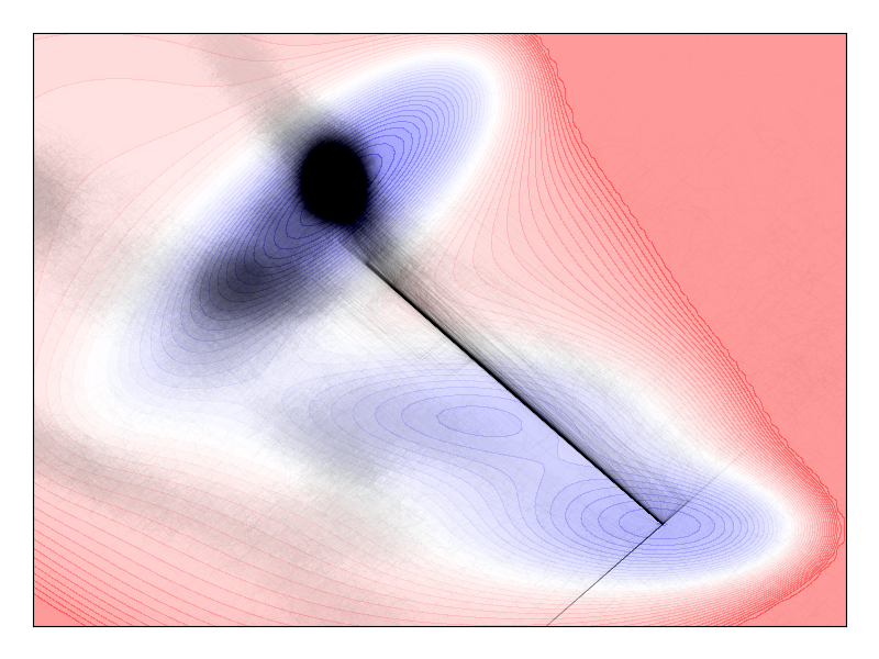
(a) TD3

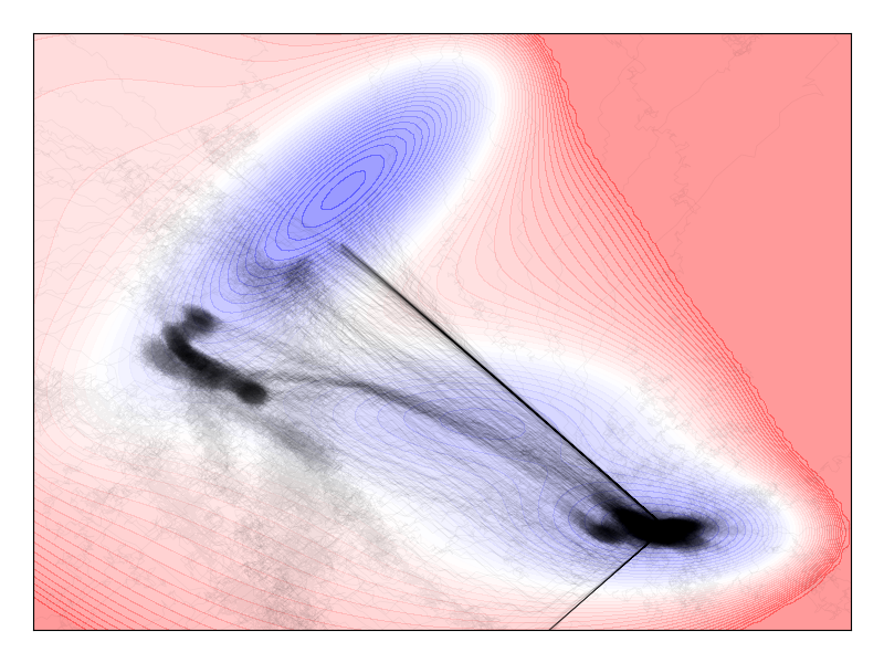
(b) SAC

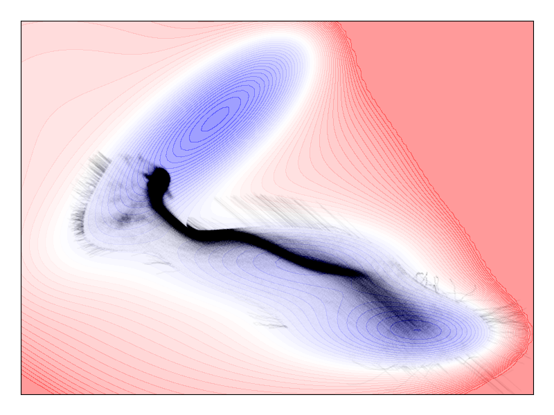
(c) Algorithm 1

Figure 4: Scatter plot of the regions visited by the reinforcement learning agent during the course of learning while using different algorithms. While TD3 (left plot) does reach the intended target, the neural nets over-fits and take a more direct path to the terminal state and hence do not give the correct estimate of the minimum energy barrier for the transition. SAC (center plot) shows an improved performance and reaches the intended target. However, while generating trajectories in the testing environment, most of the trajectories did not leave the local minima in the vicinity of the start state. Moreover, the learnt policy has a high variance. The proposed Algorithm 1 learns a much stable policy and confines itself to exploring the region with lower energies leading to the terminal state rather than the entire environment. It explores sufficiently and then exploits the state-action values learnt appropriately giving better estimates of the energy barrier for the transition.

Parameter	Value
number of dimensions ($d$)	$2$
limits for dimensions 1	$(-1.70,1.30)$
limits for dimensions 2	$(-0.40,2.10)$
scaling factor for action ($\lambda$)	$0.01$
tolerance for convergence ($\delta$)	$10^{-4}$

Table 2: Some parameters of the Markov Decision process to find pathways with the minimum energy barrier on the chosen potential.

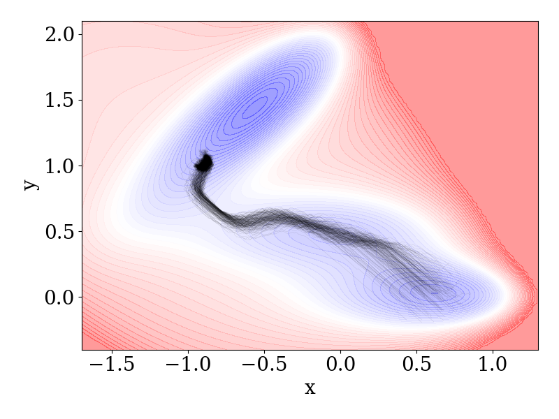
(a) Trajectories generated by the agent after training.

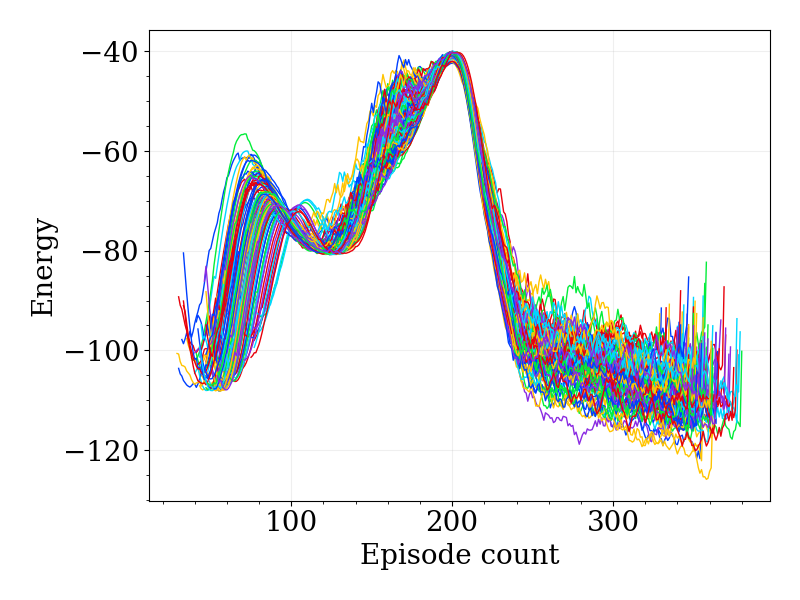
(b) Energy profiles for the generated trajectories.

Figure 5: Trajectories generated by the trained agent following the learnt policy.

In Figure 5(a), an ensemble of paths generated by the trained RL agent with the starting points slightly perturbed from $(0.623,0.028)$ by noise added from $\mathcal{N}(0,0.1)$ is plotted on the energy surface. The energy profiles along the generated trajectories are plotted in Figure 5(b) aligned by the maximum of the profiles (and not by the start of the trajectories) for better visualization. The predicted energy barrier for the transition of interest is $-40.36\pm 0.21$. One can see that the agent learns to predict the path with the correct minimum energy barrier, albeit the energy barrier estimated by the agent is a little higher than the optimal analytical solution ($-40.665$). However, the result demonstrates that reinforcement learning algorithms can be used to locate the minimum energy barrier for transitions between stable states in complex systems. The paths suggested by the trained agent cluster around the minimum energy path and pass through the vicinity of the actual saddle point representing the energy barrier. However, there still seems to be some way to go to improve the sampling densities around the saddle point, which determines the barrier height, to avoid overestimating it.

3.2 Ablation Studies

Several modifications were made to the standard SAC algorithm to be used in this particular case (highlighted in blue in Algorithm 1). Studies were performed to understand the contribution of each individual component to the working of the algorithm in this particular environment by comparing the performance of the algorithm with different hyperparameters for a component. Each modification and its contribution to the overall learning of the agent are described in the following sections. The mean and the standard deviation of the returns from the last $100$ training steps for each modification to the existing algorithm are listed in Table 6(a) to compare the performance of the agents. The modification that leads to the highest returns is highlighted.

Modification	Value	Returns
target policy	absent	$52985\pm\,\,\,\,\,\,44$
smoothing	present	$\mathbf{56241\pm\,\,453}$
	$0$	$28534\pm 8137$
	$2$	$55438\pm 1158$
policy update	$4$	$56011\pm\,\,\,931$
delay	$\mathbf{8}$	$\mathbf{56458\pm\,\,809}$
	$16$	$53666\pm\,\,\,752$
	$32$	$29309\pm\,\,\,196$
$\alpha$ tuning	$10^{-3}$	$20508\pm\,\,\,130$
	$10^{-2}$	$20950\pm\,\,\,\,\,\,60$
	$10^{-1}$	$56301\pm 3834$
	$2\times 10^{-1}$	$46376\pm 8893$
	$5\times 10^{-1}$	$49158\pm 1510$
	tunable	$\mathbf{56371\pm\,548}$

(a) Returns for the last $100$ episodes of trials
for each modification on the learning of the agent.

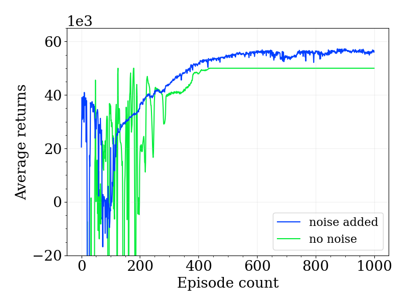
(b) Effect of adding noise to the target action
on the learning of the agent.

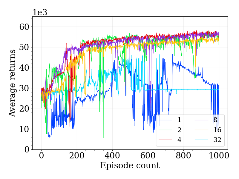
(c) Effect of delaying the update of the actor net,
and target critic-nets on the learning of the agent.

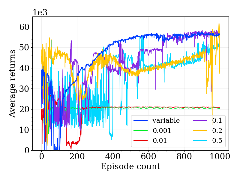
(d) Effect of varying constant values of $\alpha$ and
a tunable $\alpha$ on the learning of the agent.

Figure 6: Effect of the various modifications to the SAC algorithm on the learning of the agent.

3.2.1 Target Policy Smoothing

Injecting random noise (with a standard deviation $\sigma$) into the action used in the environment (in line 9 of Algorithm 1) encourages the agent to explore, while adding noise to the actions used to calculate the targets (in line 14 of Algorithm 1) acts as a regularizer, forcing the agent to generalize over similar actions. In the early stages of training, the critic Q-nets can assign inaccurate values to some state-action pairs, and the addition of noise prevents the actor from rote learning these actions based on incorrect feedback. On the other hand, to avoid the actor taking a too random action, the action is clipped by some maximum value for the noise (as done in lines 9 and 14 of Algorithm 1). The effect of adding noise to spread the state-action value over a range of actions is plotted in Figure 6(b). Adding noise leads to the agent learning a policy with less variance in the early learning stages and a more consistent performance.

3.2.2 Delayed Policy Updates

Delaying the updates for the actor nets and the target Q-nets (in lines 17 and 19 of Algorithm 1) allows the critic Q-nets to update more frequently and learn at a faster rate, so that they can provide a reasonable estimate of the value for a state-action pair before it is used to guide the policy learned by the actor net. The parameters of the critic Q-nets might often change abruptly early on while learning, undoing whatever the agent had learned (catastrophic failure). Therefore, delayed updates of the actor net allow it to use more stable state-action values from the critic nets to guide the policy learned by it. The effect of varying intervals of delay for the actor update on the learning of the agent is plotted in Figure 6(c). Updating the actor net for every update of the critic nets led to a policy with a high variance (blue plot). Delaying the update of the actor net to once every 2 updates of the critic resulted in the agent learning a policy that provided higher returns but still had a high variance (green plot). Delaying the update of the actor further (once every 4 and 8 updates of the critic net plotted as the red and magenta curves, respectively) further improved the performance of the agent. One can notice the lower variance in the policy of the agent during the early stages (first 200 episodes of the magenta curve) for the agent which updates the actor net and target critic nets once every 8 updates of the critic nets. However, delaying the updates for too long intervals would cripple the learning of the actor. The performance of the agent suffers when the update of the actor is delayed to once every 16 updates of the critic nets (yellow curve) and the agent fails to learn when the update of the actor net is further delayed to once every 32 updates of the critic nets (cyan curve).

3.2.3 Tuning the Entropy Coefficient

The entropy coefficient $\alpha$ can be tuned as the agent learns (as done in line 18 of Algorithm 1), which overcomes the problem of finding the optimal value for the hyperparameter $\alpha$ Haarnoja et al. [2019]. Moreover, simply fixing $\alpha$ to a single value might lead to a poor solution because the agent learns a policy over time: it should still explore regions where it has not learned the optimal action, but the policy should not change much in regions already explored by the agent that have higher returns. In Figure 6(d), the effect of the variation of the hyperparameter $\alpha$ on the learning of the agent is compared. As can be seen, a tunable $\alpha$ allows the agent to learn steadily, encouraging it to explore more in the earlier episodes and exploiting the returns from these explored regions in the latter episodes, resulting in a more stable learning curve (blue curve). A too low value of $\alpha$, such as $10^{-3}$ or $10^{-1}$, makes the algorithm more deterministic (TD3-like), which leads to sub-optimal performance and the agent being stuck in a local minimum (plotted as green and red curves, respectively). An $\alpha$ value of $0.1$ has comparable performance to the tunable $\alpha$, but the learning curve is less stable and there are abrupt changes in the policy function (magenta curve). The original implementation of SAC suggested $0.2$ as a fixed value for $\alpha$, which leads to a learning curve resulting in a policy with high variance (yellow curve). A too high value of $\alpha$, such as $0.5$, makes the algorithm more stochastic (REINFORCE-like), which also leads to sub-optimal learning (cyan curve).

4 Discussions and Conclusion

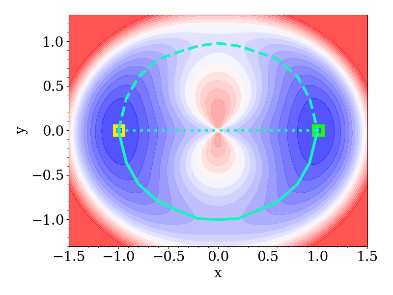
(a) A potential energy surface with pathways passing through three different saddle points.

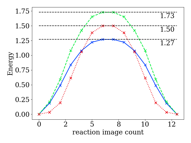
(b) The energy profiles of the three pathways depicted in (a) with their respective barrier heights.

Figure 7: (Left) Three possible pathways on a potential energy surface (taken from E et al. [2007]) passing though different saddle points. A simple interpolation between the starting and ending points would lead to the dotted trajectory. Running traditional gradient based methods would not improve this pathway as it passes through a local minima. This pathway has an energy barrier of $1.50$. The pathway with the lowest energy barrier, $1.27$, is depicted by a solid line, and was learnt by the reinforcement learning agent following Algorithm 1. (right) The energy profile for the three possible transition pathways. Nudged elastic band would have overestimated the energy barrier for the transition by $(150-127)/127$ or $18\%$, and hence underestimates the frequency with which it occurs by $1-e^{-1.50-(-1.27)}=20\%$.

Advancements in reinforcement learning algorithms based on the state-action value function have led to their application in diverse sequential control tasks such as Atari games, autonomous driving, and robot movement control. This project formulated the problem of finding the minimum energy barrier for a transition between two local minima as a cost minimization problem, solved using a reinforcement learning setup with neural networks as function approximators for the actor and critics. A stochastic policy was employed to facilitate exploration by the agent, further perturbed by random noise. Target networks, delayed updates of the actor, and a replay buffer were used to stabilize the learning process for the reinforcement learning agent. While the proposed framework samples the region around the saddle point sufficiently, providing a good estimate of the energy barrier for the transition, there is definitely scope for improvement. As future work, the method could be applied to more realistic systems.

Previous works in determining transition pathways using deep learning or reinforcement learning techniques include formulating the problem as a shooting game solved using deep reinforcement learning Zhang et al. [2021]. Additionally, in Holdijk et al. [2023], this problem is formulated as a stochastic optimal control problem, where neural network policies learn a controlled and optimized stochastic process to sample the transition pathway using machine learning techniques. Stochastic diffusion models have been used to model elementary reactions and generate the structure of the transition state, preserving the required physical symmetries in the process Duan et al. [2023]. Furthermore, the problem of finding transition pathways was recast into a finite-time horizon control optimization problem using the variational principle and solved using reinforcement learning in Guo et al. [2024]. Recent work Barrett and Westermayr [2024] used an actor-critic reinforcement learning framework to optimize molecular structures and calculate minimum energy pathways for two reactions.

This work differs from previous efforts by providing a much simpler formulation of the problem, using the energy of the state directly as the reward while searching for transition pathways with the minimum energy barrier. One of the main advantages of this method is that, unlike traditional methods such as the nudged elastic band or the growing string method, it does not require an initial guess for the transition pathway. Traditional methods use energy gradient information along the pathway to iteratively improve to a pathway with better energetics. However, the success of these methods depends on the initial guess for the pathway, which might be stuck in a local minimum, as shown in Figure 7, leading to a sub-optimal solution. This could result in an overestimate of the energy barrier and subsequently an underestimate of the probability for the transition to occur, leading to imperfect modeling of the system. On the other hand, the use of a stochastic policy in a reinforcement learning setup avoids this problem, increasing the chances of finding a better estimate of the transition barrier as the agent explores the state space. However, as a trade-off for the simple model and generic approach, the agent learns slowly and requires a large number of environment interactions.

References

- Barrett and Westermayr [2024] Rhyan Barrett and Julia Westermayr. Reinforcement learning for traversing chemical structure space: Optimizing transition states and minimum energy paths of molecules. The Journal of Physical Chemistry Letters, 15(1):349–356, 2024. doi: 10.1021/acs.jpclett.3c02771. URL https://doi.org/10.1021/acs.jpclett.3c02771. PMID: 38170921.
- Bolhuis and Swenson [2021] Peter G. Bolhuis and David W. H. Swenson. Transition path sampling as markov chain monte carlo of trajectories: Recent algorithms, software, applications, and future outlook. Advanced Theory and Simulations, 4(4):2000237, 2021. doi: https://doi.org/10.1002/adts.202000237. URL https://onlinelibrary.wiley.com/doi/abs/10.1002/adts.202000237.
- Choi [2023] S Choi. Prediction of transition state structures of gas-phase chemical reactions via machine learning. Nat Commun, 14, March 2023. doi: 10.1038/s41467-023-36823-3. URL https://doi.org/10.1038/s41467-023-36823-3.
- Duan et al. [2023] Chenru Duan, Yuanqi Du, Haojun Jia, and Heather J. Kulik. Accurate transition state generation with an object-aware equivariant elementary reaction diffusion model. Nature Computational Science, 3(12):1045–1055, Dec 2023. doi: 10.1038/s43588-023-00563-7. URL https://doi.org/10.1038/s43588-023-00563-7.
- E et al. [2007] Weinan E, Weiqing Ren, and Eric Vanden-Eijnden. Simplified and improved string method for computing the minimum energy paths in barrier-crossing events. The Journal of Chemical Physics, 126(16):164103, 04 2007. ISSN 0021-9606. doi: 10.1063/1.2720838. URL https://doi.org/10.1063/1.2720838.
- Fujimoto et al. [2018] Scott Fujimoto, Herke van Hoof, and David Meger. Addressing function approximation error in actor-critic methods, 2018. URL https://arxiv.org/abs/1802.09477.
- Goodrow et al. [2009] Anthony Goodrow, Alexis T. Bell, and Martin Head-Gordon. Transition state-finding strategies for use with the growing string method. The Journal of Chemical Physics, 130(24):244108, 06 2009. ISSN 0021-9606. doi: 10.1063/1.3156312. URL https://doi.org/10.1063/1.3156312.
- Guo et al. [2024] Jin Guo, Ting Gao, Peng Zhang, Jiequn Han, and Jinqiao Duan. Deep reinforcement learning in finite-horizon to explore the most probable transition pathway. Physica D: Nonlinear Phenomena, 458:133955, 2024. ISSN 0167-2789. doi: https://doi.org/10.1016/j.physd.2023.133955. URL https://www.sciencedirect.com/science/article/pii/S0167278923003093.
- Haarnoja et al. [2018] Tuomas Haarnoja, Aurick Zhou, Pieter Abbeel, and Sergey Levine. Soft actor-critic: Off-policy maximum entropy deep reinforcement learning with a stochastic actor, 2018. URL https://arxiv.org/abs/1801.01290.
- Haarnoja et al. [2019] Tuomas Haarnoja, Aurick Zhou, Kristian Hartikainen, George Tucker, Sehoon Ha, Jie Tan, Vikash Kumar, Henry Zhu, Abhishek Gupta, Pieter Abbeel, and Sergey Levine. Soft actor-critic algorithms and applications, 2019. URL https://arxiv.org/abs/1812.05905.
- Heinen et al. [2022] Stefan Heinen, Guido Falk von Rudorff, and O. Anatole von Lilienfeld. Transition state search and geometry relaxation throughout chemical compound space with quantum machine learning. The Journal of Chemical Physics, 157(22):221102, 12 2022. ISSN 0021-9606. doi: 10.1063/5.0112856. URL https://doi.org/10.1063/5.0112856.
- Henkelman et al. [2000] Graeme Henkelman, Blas P. Uberuaga, and Hannes Jónsson. A climbing image nudged elastic band method for finding saddle points and minimum energy paths. The Journal of Chemical Physics, 113(22):9901–9904, 12 2000. doi: 10.1063/1.1329672. URL https://doi.org/10.1063/1.1329672.
- Holdijk et al. [2023] Lars Holdijk, Yuanqi Du, Ferry Hooft, Priyank Jaini, Bernd Ensing, and Max Welling. Stochastic optimal control for collective variable free sampling of molecular transition paths, 2023. URL https://arxiv.org/abs/2207.02149.
- Jackson et al. [2021] Riley Jackson, Wenyuan Zhang, and Jason Pearson. Tsnet: predicting transition state structures with tensor field networks and transfer learning. Chem. Sci., 12:10022–10040, 2021. doi: 10.1039/D1SC01206A. URL http://dx.doi.org/10.1039/D1SC01206A.
- Jafari and Zimmerman [2017] Mina Jafari and Paul M. Zimmerman. Reliable and efficient reaction path and transition state finding for surface reactions with the growing string method. Journal of Computational Chemistry, 38(10):645–658, 2017. doi: https://doi.org/10.1002/jcc.24720. URL https://onlinelibrary.wiley.com/doi/abs/10.1002/jcc.24720.
- Jung et al. [2023] H. Jung, R. Covino, A. Arjun, et al. Machine-guided path sampling to discover mechanisms of molecular self-organization. Nat Comput Sci, 3:334–345, April 2023. doi: 10.1038/s43588-023-00428-z. URL https://doi.org/10.1038/s43588-023-00428-z.
- Koistinen et al. [2017] Olli-Pekka Koistinen, Freyja B. Dagbjartsdóttir, Vilhjálmur Ásgeirsson, Aki Vehtari, and Hannes Jónsson. Nudged elastic band calculations accelerated with Gaussian process regression. The Journal of Chemical Physics, 147(15):152720, 09 2017. ISSN 0021-9606. doi: 10.1063/1.4986787. URL https://doi.org/10.1063/1.4986787.
- Luong and Singh [2024] Kha-Dinh Luong and Ambuj Singh. Application of transformers in cheminformatics. Journal of Chemical Information and Modeling, 64(11):4392–4409, 2024. doi: 10.1021/acs.jcim.3c02070. URL https://doi.org/10.1021/acs.jcim.3c02070. PMID: 38815246.
- Makoś et al. [2021] Małgorzata Z. Makoś, Niraj Verma, Eric C. Larson, Marek Freindorf, and Elfi Kraka. Generative adversarial networks for transition state geometry prediction. The Journal of Chemical Physics, 155(2):024116, 07 2021. ISSN 0021-9606. doi: 10.1063/5.0055094. URL https://doi.org/10.1063/5.0055094.
- Mannucci and van Kampen [2016] Tommaso Mannucci and Erik-Jan van Kampen. A hierarchical maze navigation algorithm with reinforcement learning and mapping. In 2016 IEEE Symposium Series on Computational Intelligence (SSCI), pages 1–8, 2016. doi: 10.1109/SSCI.2016.7849365.
- Müller and Brown [1979] K. Müller and L.D Brown. Location of saddle points and minimum energy paths by a constrained simplex optimization procedure. Theoret. Chim. Acta, 53:75–93, March 1979. doi: 10.1007/BF00547608. URL https://doi.org/10.1007/BF00547608.
- Rotskoff et al. [2022] Grant M Rotskoff, Andrew R Mitchell, and Eric Vanden-Eijnden. Active importance sampling for variational objectives dominated by rare events: Consequences for optimization and generalization. In Joan Bruna, Jan Hesthaven, and Lenka Zdeborova, editors, Proceedings of the 2nd Mathematical and Scientific Machine Learning Conference, volume 145 of Proceedings of Machine Learning Research, pages 757–780. PMLR, 16–19 Aug 2022. URL https://proceedings.mlr.press/v145/rotskoff22a.html.
- Sutton and Barto [1998] R.S. Sutton and A.G. Barto. Reinforcement Learning: An Introduction. A Bradford book. MIT Press, 1998. ISBN 9780262193986. URL https://books.google.dk/books?id=CAFR6IBF4xYC.
- Towers et al. [2023] Mark Towers, Jordan K. Terry, Ariel Kwiatkowski, John U. Balis, Gianluca de Cola, Tristan Deleu, Manuel Goulão, Andreas Kallinteris, Arjun KG, Markus Krimmel, Rodrigo Perez-Vicente, Andrea Pierré, Sander Schulhoff, Jun Jet Tai, Andrew Tan Jin Shen, and Omar G. Younis. Gymnasium, March 2023. URL https://zenodo.org/record/8127025.
- Vlachas et al. [2022] Pantelis R. Vlachas, Julija Zavadlav, Matej Praprotnik, and Petros Koumoutsakos. Accelerated simulations of molecular systems through learning of effective dynamics. Journal of Chemical Theory and Computation, 18(1):538–549, 2022. doi: 10.1021/acs.jctc.1c00809. URL https://doi.org/10.1021/acs.jctc.1c00809. PMID: 34890204.
- Wander et al. [2024] Brook Wander, Muhammed Shuaibi, John R. Kitchin, Zachary W. Ulissi, and C. Lawrence Zitnick. Cattsunami: Accelerating transition state energy calculations with pre-trained graph neural networks, 2024. URL https://arxiv.org/abs/2405.02078.
- Zhang et al. [2021] Jun Zhang, Yao-Kun Lei, Zhen Zhang, Xu Han, Maodong Li, Lijiang Yang, Yi Isaac Yang, and Yi Qin Gao. Deep reinforcement learning of transition states. Phys. Chem. Chem. Phys., 23:6888–6895, 2021. doi: 10.1039/D0CP06184K. URL http://dx.doi.org/10.1039/D0CP06184K.