Variable-Agnostic Causal Exploration for Reinforcement Learning
Abstract
Modern reinforcement learning (RL) struggles to capture real-world cause-and-effect dynamics, leading to inefficient exploration due to extensive trial-and-error actions. While recent efforts to improve agent exploration have leveraged causal discovery, they often make unrealistic assumptions of causal variables in the environments. In this paper, we introduce a novel framework, Variable-Agnostic Causal Exploration for Reinforcement Learning (VACERL), incorporating causal relationships to drive exploration in RL without specifying environmental causal variables. Our approach automatically identifies crucial observation-action steps associated with key variables using attention mechanisms. Subsequently, it constructs the causal graph connecting these steps, which guides the agent towards observation-action pairs with greater causal influence on task completion. This can be leveraged to generate intrinsic rewards or establish a hierarchy of subgoals to enhance exploration efficiency. Experimental results showcase a significant improvement in agent performance in grid-world, 2d games and robotic domains, particularly in scenarios with sparse rewards and noisy actions, such as the notorious Noisy-TV environments.
Keywords: Reinforcement Learning, Causality, Deep RL.
1 Introduction
Reinforcement learning (RL) is a machine learning paradigm wherein agents learn to improve decision-making over time through trial and error [25]. While RL has demonstrated remarkable success in environments with dense rewards [15, 23], it tends to fail in case of sparse rewards where the agents do not receive feedback for extended periods, resulting in unsuccessful learning. Such scarcity of rewards is common in real-world problems: e.g., in a search mission, the reward is only granted upon locating the target. Prior studies tackle this problem by incentivizing exploration through intrinsic rewards [26, 3], motivating exploration of the unfamiliar, or with hierarchical reinforcement learning (HRL) [13, 31, 17]. However, these methods encounter difficulties when scaling up to environments with complex structures as they neglect the causal dynamics of the environments. Consider the example of a search in two rooms (Fig. 1(a, b)), where the target is in the second room, accessible only by opening a “door” with a “key” in the first room. Traditional exploration methods might force the agent to explore all corners of the first room, even though only the “key” and “door” areas are crucial. Knowing that the action "pick up key" is the cause of the effect "door opened" will prevent the agent from aimlessly wandering around the door before the key is acquired. Another challenge with these approaches is the Noisy-TV problem [3], where the agent excessively explores unfamiliar states and actions that may not contribute to the ultimate task. These inefficiencies raise a new question: Can agents effectively capture causality to efficiently explore environments with sparse rewards and distracting actions?
Inspired by human reasoning, where understanding the relationship between the environmental variables (EVs) helps exploration, causal reinforcement learning (CRL) is grounded in causal inference [29]. CRL research often involves two phases: (i) causal structure discovery and (ii) integrating causal knowledge with policy training [29]. Recent studies have demonstrated that such knowledge significantly improves the sample efficiency of agent training [8, 22, 30]. However, current approaches often assume assess to all environmental causal variables and pre-factorized environments [22, 8], simplifying the causal discovery phase. In reality, causal variables are not given from observations, and constructing a causal graph for all observations becomes a non-trivial task due to the computational expense associated with measuring causality. Identifying EVs crucial for downstream tasks becomes a challenging task, thereby limiting the effectiveness of CRL methods. These necessitate the identification of a subset of crucial EVs before discovering causality.
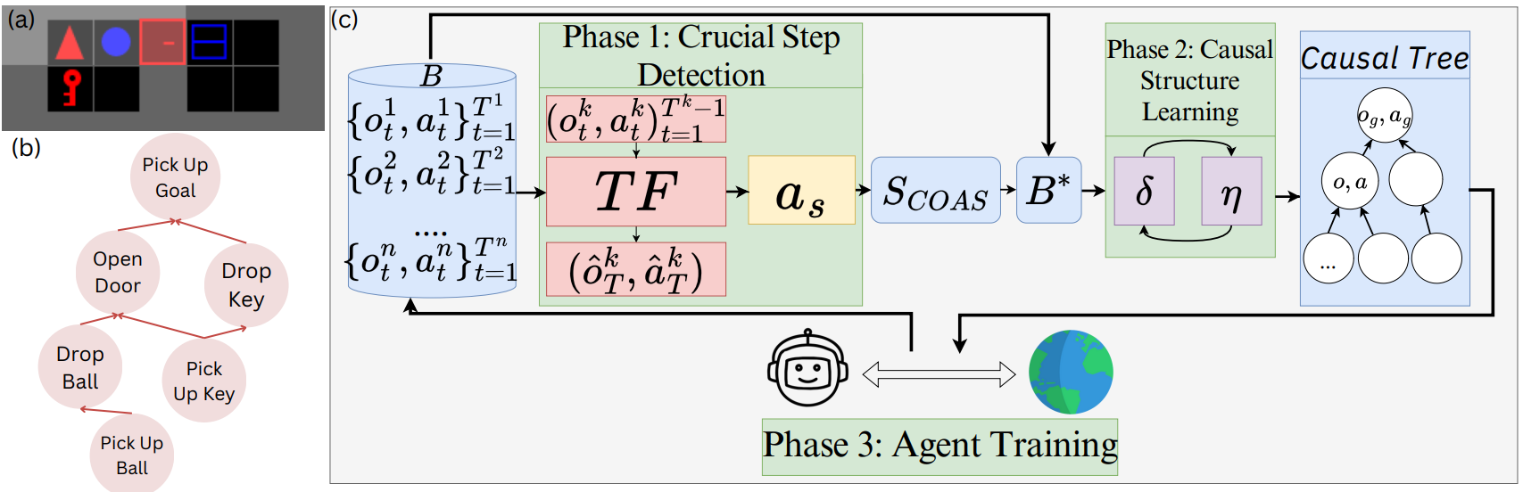
This paper introduces the Variable-Agnostic Causal Exploration for Reinforcement Learning (VACERL) framework to address these limitations. The framework is an iterative process consisting of three phases: “Crucial Step Detection”, “Causal Structure Discovery”, and “Agent Training with Causal Information”. The first phase aims to discover a set of crucial observation-action steps, denoted as the . The term “crucial observation-action step” refers to an observation and an action pair stored in the agent’s memory identified as crucial for constructing the causal graph. We extend the idea of detecting crucial EVs to detecting crucial observation-action steps, motivated by two reasons. Firstly, variables in the environment are associated with the observations, e.g., the variable “key” corresponds to the agent’s observation of the “key”. Secondly, actions also contribute to causality, e.g., the agent cannot use the “key” without picking it up. One way of determining crucial observation-action steps involves providing the agent with a mechanism to evaluate them based on their contribution to a meaningful task [9]. We implement this mechanism using a Transformer architecture, whose task is to predict the observation-action step leading to the goal given past steps. We rank the significance of observation-action steps based on their attention scores [28] and pick out the top-ranking candidates since the Transformer must attend to important steps to predict correctly.
In Phase 2, we adapt causal structure learning [10] to discover the causal relationships among the observation-action steps identified in the discovered set, forming a causal graph . The steps serve as the nodes of the causal graph, while the edges can be identified through a two-phase iterative optimization of the functional and structural parameters, representing the Structure Causal Model (SCM). In Phase 3, we train the RL agent based on the causal graph . To prove the versatility of our approach in improving the sample efficiency of RL agents, we propose two methods to utilize the causal graph: (i) formulate intrinsic reward-shaping equations grounded on the captured causal relationship; (ii) treat the nodes in the causal graph as subgoals for HRL. During subsequent training, the updated agent interact with the environments, collecting new trajectories for the agent memory used in the next iteration of Phase 1.
In our experiments, we use causally structured grid-world and robotic environments to empirically evaluate the performance improvement of RL agents when employing the two approaches in Phase 3. This improvement extends not only to scenarios with sparse rewards but also to those influenced by the Noisy-TV problem. We also investigate the contributions of the core components of VACERL, analyzing the emerging learning behaviour that illustrates the captured causality of the agents. Our main contributions can be summarized as:
-
•
We present a novel VACERL framework, which autonomously uncovers causal relationships in RL environments without assuming environmental variables or factorized environments.
-
•
We propose two methods to integrate our framework into common RL algorithms using intrinsic reward and hierarchical RL, enhancing exploration efficiency and explaining agent behaviour.
-
•
We create causally structured environments, with and without Noisy-TV, to evaluate RL agents’ exploration capabilities, demonstrating the effectiveness of our approach through extensive experiments.
2 Related Work
Causal Reinforcement Learning (CRL) is an emerging field that integrates causality and reinforcement learning (RL) to enhance decision-making in RL agents, addressing limitations associated with traditional RL, such as sample efficiency and explainability [29]. CRL methods can be categorized based on their experimental setups, whether they are online or offline [29]. Online-CRL involves real-time interaction with the environment [5, 8, 30, 22], while Offline-CRL relies on learning from a fixed previously collected dataset [24, 18]. Our framework operates online, using trajectories from an online policy for an agent training while simultaneously constructing the underlying causal graph. Prior works in CRL have focused on integrating causal knowledge into RL algorithms and building causal graphs within the environment. Pitis et al., [18] use Transformer model attention weights to generate counterfactual data for training RL agents, while Coroll et al., [5] use causal effect measurement to build a hierarchy of controllable effects. Zhang et al., [32] measure the causal relationship between states and actions with the rewards and redistribute the rewards accordingly. For exploration purposes, CRL research integrates causal knowledge by rewarding the agents when they visit states with higher causal influence [22, 30] or treating the nodes of the causal graph as potential subgoals in HRL [8]. Zhang et al., [30] measure the average causal effect between a predefined group of variables and use this as a reward signal, meanwhile, Seitzer et al., [22] propose conditional mutual information as a measurement of causal influence and use it to enhance the exploration of the RL agent. Hu et al., [8] introduce a continuous optimization framework, building a causal structure through a causality-guided intervention and using it to define hierarchical subgoals. Despite advancements, previous methods often assume prior knowledge of EVs and the ability to factorize the environment accordingly. Our framework autonomously detects crucial steps associated with the key EVs, enabling causal structure learning without predefined EVs, thus, distinguishing it from previous methods. The causal graph uncovered by VACERL is versatile and can complement existing RL exploration methods, such as intrinsic reward motivation or as hierarchical subgoals.
Intrinsic Reward Motivation addresses inefficient training in sparse reward RL environments; an issue associated with random exploration techniques like -greedy [2]. The core idea underlying these motivation strategies is to incorporate intrinsic rewards, which entail adding bonuses to the environment rewards to facilitate exploration [2, 26, 3]. These methods add bonuses to environment rewards to encourage exploration, either based on prediction error [3] or count-based criteria [2, 26]. However, they struggle to scale to complex structure environments, especially in the scenario of Noisy-TV, where the agent becomes excessively curious about unpredictable states and ignores the main task [3]. VACERL tackles this by incorporating a mechanism to identify essential steps for the primary task and construct the causal graph around these steps, thus, enabling the agent to ignore actions generating noisy-TV.
Goal-conditioned Hierarchical Reinforcement Learning (HRL) is another approach that is used to guide agent exploration. Levy et al., [13] propose a multilevel policies framework, in which each policy is trained independently and the output of higher-ranking policies are used as subgoals for lower-level policies. Zhang et al., [31] propose an adjacency constraint method to restrict the search space of subgoals, whereas, Pitis et al., [17] introduce a method based on maximum entropy gain motivating the agent to pursue past achieved goals in sparsely explored areas. However, traditional HRL methods often rely on random subgoals exploration, which has shown inefficiency in learning high-quality hierarchical structures compared to causality-driven approaches [8, 7]. Hu et al., [8] operate under the assumption of pre-availability and disentanglement of causal EVs from observations, using these EVs as suitable subgoals for HRL. However, they overlook cases where these assumptions are not applicable, e.g., the observation is the image. In our apprroach, subgoals are determined by abstract representations of the observation and action, thereby, extending the applications of causal HRL to unfactorized environments.
3 Methods
3.1 Background
RL Preliminaries.
We are concerned with the Partially Observable Markov Decision Process (POMDP) framework, denoted as the tuple . The framework includes sets of states actions , observations providing partial information of the true state, a transition probability function , and an observation model denoted as , indicating the probability of observing when taking action in state . is a reward function that defines the immediate reward that the agent receives for taking an action in a given state, and discount factor . The objective of the RL agent is to maximize the expected discounted cumulative reward , over a policy function mapping a state to a distribution over actions.
Causality.
Causality is explored through the analysis of relationships among variables and events [16]. It can be described using the SCM framework [16]. SCM, for a finite set comprising variables, is where denotes the set of generating functions based on the causal graph and represents the set of noise in the model. The graph provides the edge , representing variable causes on variable , where if , else, . The SCM framework can be characterized by two parameter sets: the functional parameter , representing the generating function ; the structural parameter , modelling the adjacency matrix of [10].
3.2 Variable-Agnostic Causal Exploration Reinforcement Learning Framework
3.2.1 Overview.
The primary argument of VACERL revolves around the existence of a finite set of environment variables (EVs) that the agent should prioritize when constructing the causal graph. We provide a mechanism to detect these variables, aiming to reduce the number of nodes in the causal graph mitigating the complexity of causal discovery. Initially, we deploy an agent to randomly explore the environment and gather successful trajectories. Once the agent accidentally reaches the goal a few times, we initiate Phase 1, reformulating EVs detection into finding the “crucial observation-action steps” () from the collected trajectories. The agent is equipped with the ability to rank the importance of these steps by employing the Transformer () model’s attention scores (). Top- highest-score steps will form the crucial set . Subsequently, in Phase 2, we identify the causal relationships among steps in to learn the causal graphs of the environment. In Phase 3, where we extract a hierarchy causal tree from graph and use it to design two approaches, enhancing the RL agent’s exploration capability. We then utilize the updated agent to gather more successful trajectories and repeat the process from Phase 1. See Fig. 1(c) for an overview of VACERL and detailed implementation in Supp. A 111The source is available at https://github.com/mhngu23/Variable-Agnostic-Causal-Exploration-for-Reinforcement-Learning-VACERL.
3.2.2 Phase 1: Crucial Step Detection.
We hypothesize that important steps (a step is a pair of observation and action) are those in the agent’s memory that the agent must have experienced to reach the goal. Hence, these steps should be found in trajectories where the agent successfully reaches the goal. We collect a buffer , where is the number of episodes wherein the agent successfully reaches the goal state, and is the observation and action, respectively at step in an episode, and is the number of steps in the -th episode. We train the model, whose input consists of steps from the beginning to the second-to-last step in each episode and the output is the last step. The reasoning behind choosing the last step as the prediction target is that it highlights which steps in the trajectories are crucial for successfully reaching the goal. For a training episode -th sampled from we predict . The model is trained to minimize the loss , where is the mean square error. Following training, we rank the significant observation-action steps based on their attention scores (detailed in Supp. A)
and pick out the top- highest-score steps. We argue that the top-attended steps should cover crucial observations and actions that contribute to the last step prediction task, associated with meaningful causal variables. For instance, observing the key and the action of picking it up are linked to the variable “key”.
In continuous state space, the agent may repeatedly attend to similar steps involving the same variable. For example, the agent might select multiple instances of observing the key, from different positions where the agent is located, and picks it up. As a result, the set will be filled with similar steps relating to picking up the key and ignoring other important steps. To address this, we introduce a function to decide if two steps are the same:
-
•
For discrete action space environments,
if and , else . -
•
For continuous action space environments, if , else .
where and is a similarity threshold. Intuitively, if the agent has two observations with a high cosine similarity and takes the same action, these instances are grouped. The score for a group is the highest among the steps in this group. The proposed method will also be effective in noisy environments, particularly when the observations are trained representations rather than raw pixel data. Subsequently, we add the steps with the highest to . We define an abstract function to map a pair to an element in : and collect a new buffer , where:
| (1) |
Here, is removing steps that are unimportant (not in ).
3.2.3 Phase 2: Causal Structure Discovery.
Inspired by the causal learning method proposed by Ke et al., [10], we uncover the causal relationships among steps identified in the set. Our approach optimizes the functional parameter and the structural parameter associated with the SCM framework. The optimization of these parameters follows a two-phase iterative update process, wherein one parameter is fixed while the other is updated. Both sets of parameters are initialized randomly and undergo training using the buffer (Eq. 1). Our intuition for training the SCM is that the “cause” step has to precede its “effect” step. Therefore, we train the model to predict the step at timestep using the sequence of steps leading to that particular timestep.
In the first causal discovery phase, we fix and optimize . For a step in the trajectory -th, we formulate as:
| (2) |
where is the sequence of steps from to that belong to the parental set of , as defined by the current state of parameterized by . We use MSE as the loss function:
| (3) |
In the second phase, we fix and optimize the parameter by updating the causality from variable to as , where indicates the -th drawn sample of causal graph , given the current parameter , and is the update rate. is the edge from variable to of , and is the sigmoid function. is the MSE loss in Eq. 3 for specific variable of current function under graph . After updating parameter for a number of steps, we repeat the optimization process of parameter . Finally, we use the resulting structural parameter to construct the causal graph . We derive edge of graph , using:
| (4) |
where is the causal threshold.
3.2.4 Phase 3: Agent Training with Causal Information.
We extract a refined hierarchy causal tree from graph with an intuition to focus on steps that are relevant to achieving the goal. Using the goal-reaching step as the root node of the tree, we recursively determine the parental steps of this root node within graph , and subsequently for all identified parental steps. This causal tree is used to design causal exploration approaches. These approaches include (i) intrinsic rewards based on the causal tree, and (ii) utilizing causal nodes as subgoals for HRL. For the first approach, we devise a reward function where nodes closer to the root are deemed more important and receive higher rewards, preserving the significance of the reward associated with the root node and maintaining the agent’s focus on the goal. In the second approach, subgoals are sampled from nodes in the causal tree, with nodes closer to the root sampled more frequently. We present the detailed implementations and empirically evaluate these approaches in Sec. 4.1 and Sec. 4.2.
4 Experiments
4.1 VACERL: Causal Intrinsic Rewards - Implementation and Evaluation
Causal Intrinsic Reward.
To establish the relationship where nodes closer to the goal hold greater importance, while ensuring the agent remains focused on the goal, we introduce intrinsic reward formulas as follows:
| (5) |
where is the reward given when the agent reach the goal, is the intrinsic reward given to a node , is the set of nodes at depth of the tree, with is a hyperparameter and is the tree height. In the early learning stage, especially for hard exploration environments, the causal graph may not be well defined and thus, may not provide a good incentive. To mitigate this issue, we augment with a count-based intrinsic reward, aiming to accelerate the early exploration stage. Intuitively, the agent is encouraged to visit never-seen-before observation-action pairs in early exploration. Notably, unlike prior count-based methods [2], we restrict counting to steps in , i.e., only crucial steps are counted. Our final intrinsic reward is:
| (6) |
where is the number of time observation and action is encountered up to time step . Starting from zero, this value increments with each subsequent encounter. We add the final intrinsic reward to the environment reward to train the policy. The total reward is , where is the extrinsic reward provided by the environment.
Environments.
We perform experiments across three sets of environments: FrozenLake (FL), Minihack (MH), and Minigrid (MG). These environments are tailored to evaluate the approach in sparse reward settings, where the agent receives a solitary +1 reward upon achieving the goal (detailed in Supp. B)
FL includes the 4x4 (4x4FL) and 8x8 (8x8FL) FrozenLake environments (Supp Fig. B.1(d,e)) [27]. Although these are classic navigation problems, hidden causal relationships exist between steps. The pathway of the agent can be conceptualized as a causal graph, where each node represents the agent’s location cell and its corresponding action. For example, moving right from the cell on the left side of the lake can be identified as the cause of the agent falling into the lake cell. We use these environments to test VACERL’s efficiency in discrete state space, where is not used.
MH includes MH-1 (Room), MH-2 (Room-Monster), MH-3 (Room-Ultimate) and MH-4 (River-Narrow) [20]. These environments pose harder exploration challenges compared to FL due to the presence of more objects. Some environments even require interaction with these objects to reach the goal, such as killing monsters (MH-2 and MH-3) or building bridges (MH-4). For this set of environments, we use pixel observations.
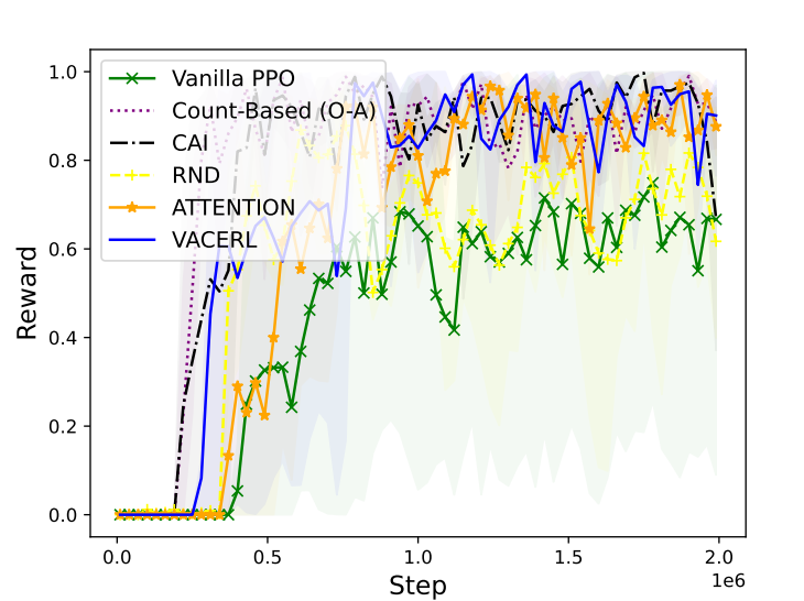
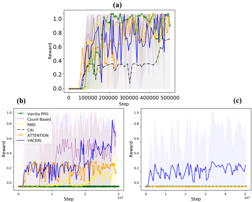
MG is designed based on Minigrid Environment [4], with escalating causality levels. These include the Key Corridor (MG-1) (Supp. Fig. B.1(a)) and 3 variants of the BlockUnlockPickUp: 2 2x2 rooms (MG-2 Fig. 1(a)), 2 3x3 rooms (MG-3) and the 3 2x2 rooms (MG-4) (Supp Fig. B.1(b,c)). The task is to navigate and locate the goal object, in a different room. These environments operate under POMDP, enabling us to evaluate the framework’s ability to construct the causal graph when only certain objects are observable at a timestep. In these environments, the agent completes the task by following the causal steps: firstly, remove the obstacle blocking the door by picking it up and dropping it in another position, then, pick up the key matching the colour of the door to open it; and finally, pick up the blue box located in the rightmost room, which is the goal. In MG-3, distracting objects are introduced to distract the agent from this sequence of action. In any case, intrinsic exploration motivation is important to navigate due to reward sparsity; however, blind exploration without an understanding of causal relationships can be ineffective.
Noisy-TV setting is implemented as an additional action (action to watch TV) and can be incorporated into any of the previous environments, so the agent has the option to watch the TV at any point while navigating the map [12]. When taking this watching TV action, the agent will be given white noise observations sampled from a standard normal distribution. As sampled randomly, the number of noisy observations can be conceptualized as infinite.
Baselines.
PPO [21], a policy gradient method, serves as the backbone algorithm of our method and other baselines. Following Schulman et al., [21], vanilla PPO employs a simple entropy-based exploration approach. Other baselines are categorized into causal and non-causal intrinsic motivation. Although our focus is causal intrinsic reward, we include non-causal baselines for comprehensiveness. These include popular methods: Count-based [2, 26] and RND [3]. Causal motivation baselines include ATTENTION and CAI, which are two methods that have been used to measure causal influence [22, 18]. We need to adapt these methods to follow our assumption of not knowing causal variables. The number of steps used to collect initial successful trajectories and to reconstruct the causal graph (denoted as and respectively) for VACERL and causal baselines are provided for each environment in Supp. D. However, not all causal methods can be adapted, and as such, we have not conducted comparisons with approaches, such as [8]. Additionally, as we do not require demonstrating trajectory from experts, we do not compare with causal imitation learning methods [6, 24].
Results.
In this section, we present our empirical evaluation results of VACERL with causal intrinsic rewards.
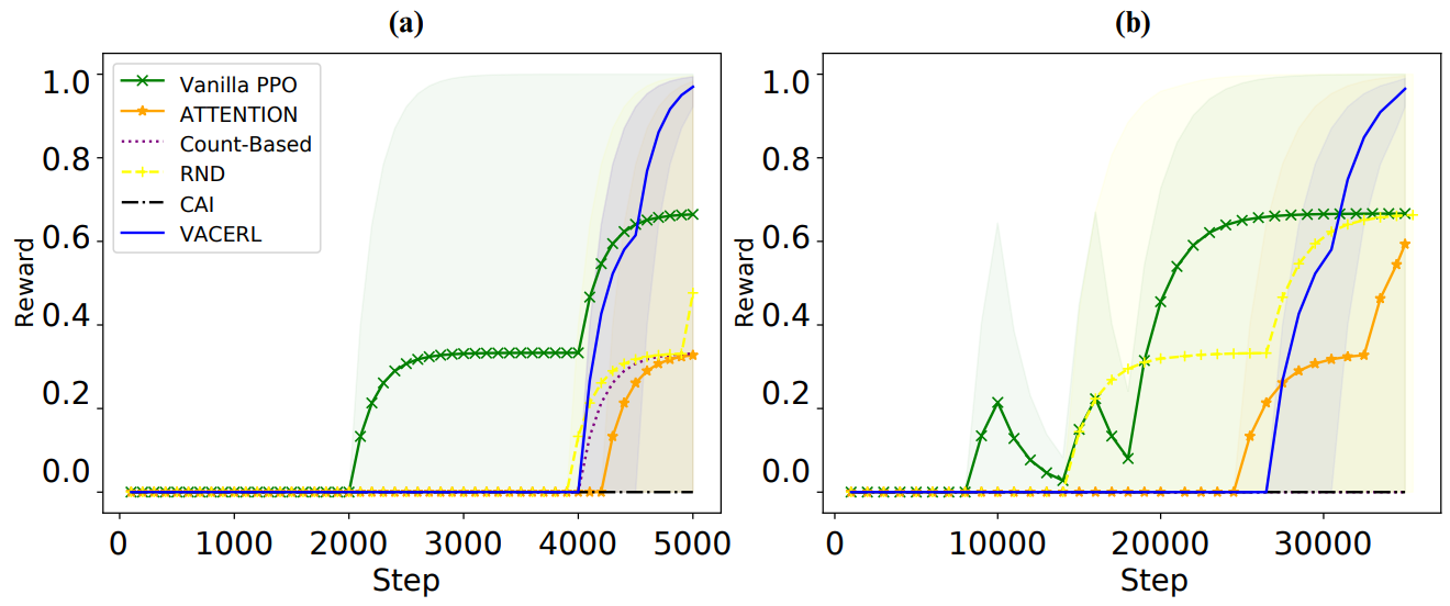
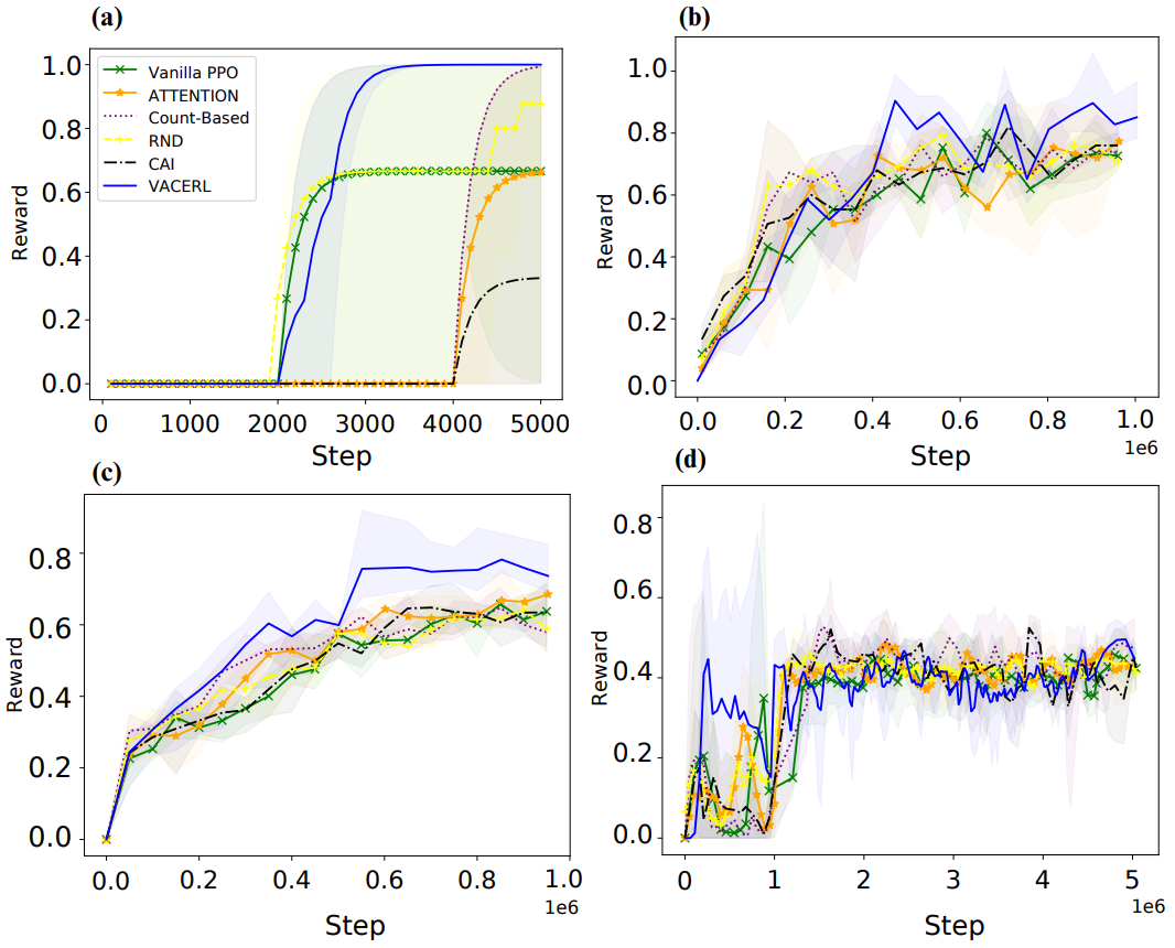
Discrete State Space: Table 1 illustrates that our rewards improve PPO’s performance by approximately 30%, in both 4x4FL and 8x8FL environments. Notably, VACERL outperforms both causal baselines, ATTENTION and CAI. Specifically, VACERL surpasses ATTENTION by 67% and 39% in 4x4FL and 8x8FL. CAI fails to learn the tasks within the specified steps due to insufficient trajectories in the agent’s memory for precise causality estimation between all steps. In contrast, our method, incorporating a crucial step detection phase, requires fewer trajectories to capture meaningful causal relationships in the environment. VACERL also performs better than Count-based by 66% in 4x4FL and 100% in 8x8FL, and RND by 51% in 4x4FL and 31% in 8x8FL. We hypothesize that Count-based and RND’s intrinsic rewards are unable to encourage the agent to avoid the trapping lakes, unlike VACERL’s are derived from only successful trajectories promoting safer exploration.
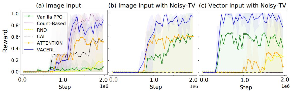
MG-2 Learning Curve Analysis: We conduct experiments with 2 types of observation space (image and vector) and visualize the learning curves in Fig. 2(a) and Supp. Fig. B.4. Results demonstrate that VACERL outperforms vanilla PPO, causal baselines, and RND in both types of observation space. While VACERL shows slightly slower progress than Count-based in early steps, it quickly catches up in later stages, ultimately matching optimal performance. We attribute this to VACERL requires a certain number of training steps to accurately acquire the causal graph before the resulting causal rewards influence the agent’s training—a phenomenon observed in other causal baselines as well.
Continuous State Space: Table 1 summarizes the testing results on 8 continuous state space environments (MH-1 to MG-4). In most of these environments, VACERL demonstrates superior performance. It only ranks as the second-best in MH-4, MG-1 and MG-2 with competitive returns. In MG-3 environment, at 30 million steps, VACERL achieves the best result with an average return of 0.77, outperforming the second-best Count-based by 10%, while other baselines show little learning. Notably, in the hardest task MG-4, only VACERL can show signs of learning, achieving an average score of 0.29 after 50 million steps whereas other baselines’ returns remain zero. Additional learning curves and results are provided in Supp. B.
Under Noisy-TV: Fig. 2(b, c), showing the results on MG-2 environment under Noisy-TV setting, confirm that our reward exhibits greater robustness in Noisy-TV environments compared to traditional approaches. Count-based, CAI, and RND fail in this setting as they cannot differentiate noise from meaningful novelty, thus, getting stuck watching Noisy-TV. While the noise less impacts ATTENTION and naive PPO, their exploration strategies are not sufficient for sparse reward environments. Overall, VACERL is the only method performing well across all settings, with or without Noisy-TV.
| Task | Step (,000) | PPO | Count-Based | RND | ATTENTION | CAI | VACERL |
|---|---|---|---|---|---|---|---|
| 4x4FL | 5 | ||||||
| 8x8FL | 35 | ||||||
| MH-1 | 5 | ||||||
| MH-2 | 1,000 | ||||||
| MH-3 | 1,000 | ||||||
| MH-4 | 5,000 | ||||||
| MG-1 | 500 | ||||||
| MG-2 | 2,000 | ||||||
| MG-3 | 30,000 | ||||||
| MG-4 | 50,000 |
4.2 VACERL: Causal Subgoals - Implementation and Evaluation
Causal subgoals sampling.
In HRL, identifying subgoals often relies on random exploration [13, 31], which can be inefficient in large search spaces. We propose leveraging causal nodes as subgoals, allowing agents to actively pursue these significant nodes. To incorporate causal subgoals into exploration, we suggest substituting a portion of the random sampling with causal subgoal sampling. Specifically, in the HRL method under experimentation where subgoals are randomly sampled 20% of the time, we replace a fraction of this 20% with a node from the causal tree as a subgoal, while retaining random subgoals for the remainder. Eq. 7 denotes the probability of sampling a node at depth (excluding the root node as this is the ultimate goal) from the causal tree:
| (7) |
with is the depth of node and is the number of nodes in the causal tree.
Environments.
We use FetchReach and FetchPickAndPlace environments from Gymnasium-Robotics [11]. These are designed to test goal-conditioned RL algorithms. We opt for sparse rewards settings, in which only a single reward of is given if the goal is met, otherwise (detailed in Supp. C).
Baselines.
HAC [13], a goal-conditioned HRL algorithm, serves as the backbone and a baseline. HAC is implemented as a three-level DDPG [14] with Hindsight Experience Replay (HER) [1], where the top two levels employ a randomized mechanism for subgoal sampling. We also evaluate our performance against the standard DDPG+HER algorithm [1] on the FetchPickAndPlace environment, as this is the more challenging task [19] and for comprehensiveness.
Results.
In this section, we outline our empirical evaluation results of VACERL with causal subgoals.
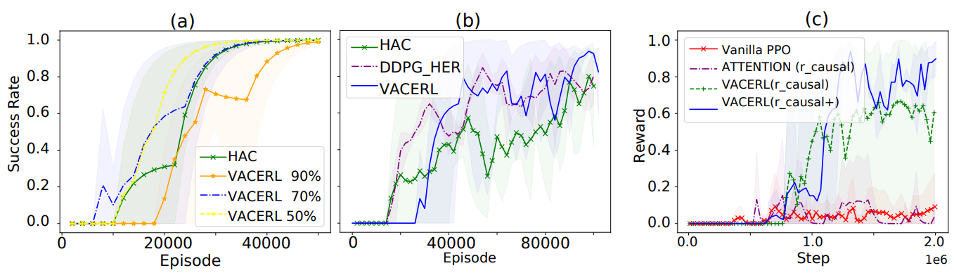
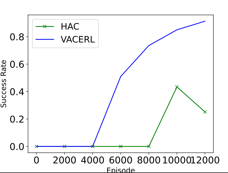
FetchReach: We assess the impact of replacing varying proportions of random sampling subgoals with nodes from the causal graph, based on Eq. 7, on the performance of the HRL agent. The learning curve in Fig. 3(a) suggests that replacing with percentages of 50% and 70% enhances the sample efficiency of the Vanilla HAC. Notably, when employing a 70% substitution rate, agents demonstrate signs of learning after only 4,000 episodes, a considerable improvement over the HAC agent’s 10,000 episodes. Conversely, replacing 50% leads to a swifter convergence, at 20,000 episodes comparing to HAC at 25,000 episodes. Additional experiments (Supp. C) demonstrate that this accelerated convergence rate is attributable to the learned causal subgoals. In contrast, employing a 90% substitution rate results in a decline in performance. We assert that this decline comes from insufficient exploration of new subgoals, leading to an inadequate number of trajectories in buffer for causal discovery.
FetchPickAndPlace: We adopt the 50% replacement, which yielded the most stable performance in the FetchReach environment for this environment. The learning curve of VACERL in Fig. 3(b) shows a similar pattern to the learning curves for the MG-2 task in Fig. 2(a). VACERL progresses slower but eventually achieves optimal performance, surpassing DDPG+HER and HAC after 90,000 episodes. In this environment, we reconstruct the causal tree every 10,000 episodes, and as seen in the learning curve, the RL agent’s performance begins to improve after approximately 20,000 episodes (worst case improves after 40,000 episodes).
4.3 Ablation Study and Model Analysis
We use MG-2 (Fig. 1(a)) task and causal intrinsic reward for our analysis.
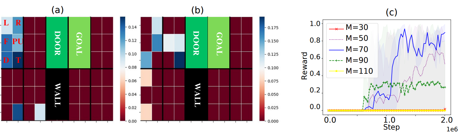
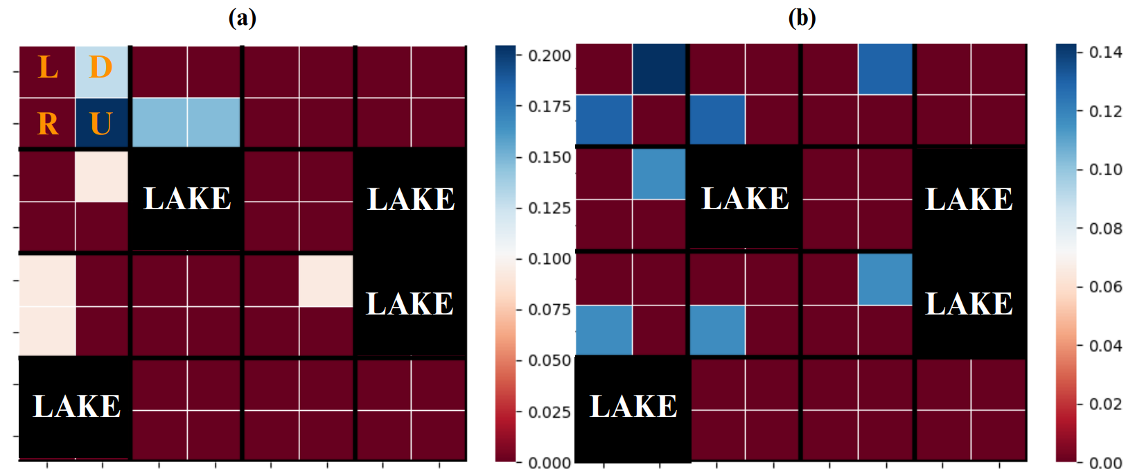
Crucial Step Detection Analysis: We investigate how the the Transformer model ’s performance changes with varying buffer sizes. As depicted in Fig. 4(a,b), increasing the number of trajectories in enhances the framework’s accuracy in detecting important steps through attention. Initially, with 4 trajectories (Fig. 4(a)), attends to all actions in the top-left grid. However, after being trained with 40 trajectories (Fig. 4(b)), correctly attends to pick-up action (PU) in the top-left grid, corresponding to the key pickup event. It can also attend to toggle action (T) in front of the door, corresponding to using the key to open the door. Additional visualization for 4x4FL is in Supp. Fig. B.6.
Next, we investigate the effects of employing varying sizes of (). The results in Fig. 4(c) reveal that varying changes the performance of the agent drastically. If is too small, the agent will not be able to capture all causal relations, thereby failing to mitigate the issue of sparse reward. On the other hand, too large can be noisy for the causal discovery phase as the causal graph will have redundant nodes. We find that the optimal value for , in MG-2, is 70, striking a balance between not being too small or too large.
Intrinsic Reward Shaping Analysis: We exclude the counting component (Eq. 6) from the final intrinsic reward to assess the agent’s exploration ability simply based on . The results in Fig. 3(c) show that the agent remains proficient relying only on the causally motivated reward (green curve). In particular, in the absence of Eq. 6, the VACERL agent still outperforms Vanilla PPO. However, its performance is not as optimal as the full VACERL (, blue curve). This is because, in early iteration, the causal graph is not yet well defined, diminishing the efficiency of solely using the causal intrinsic reward .
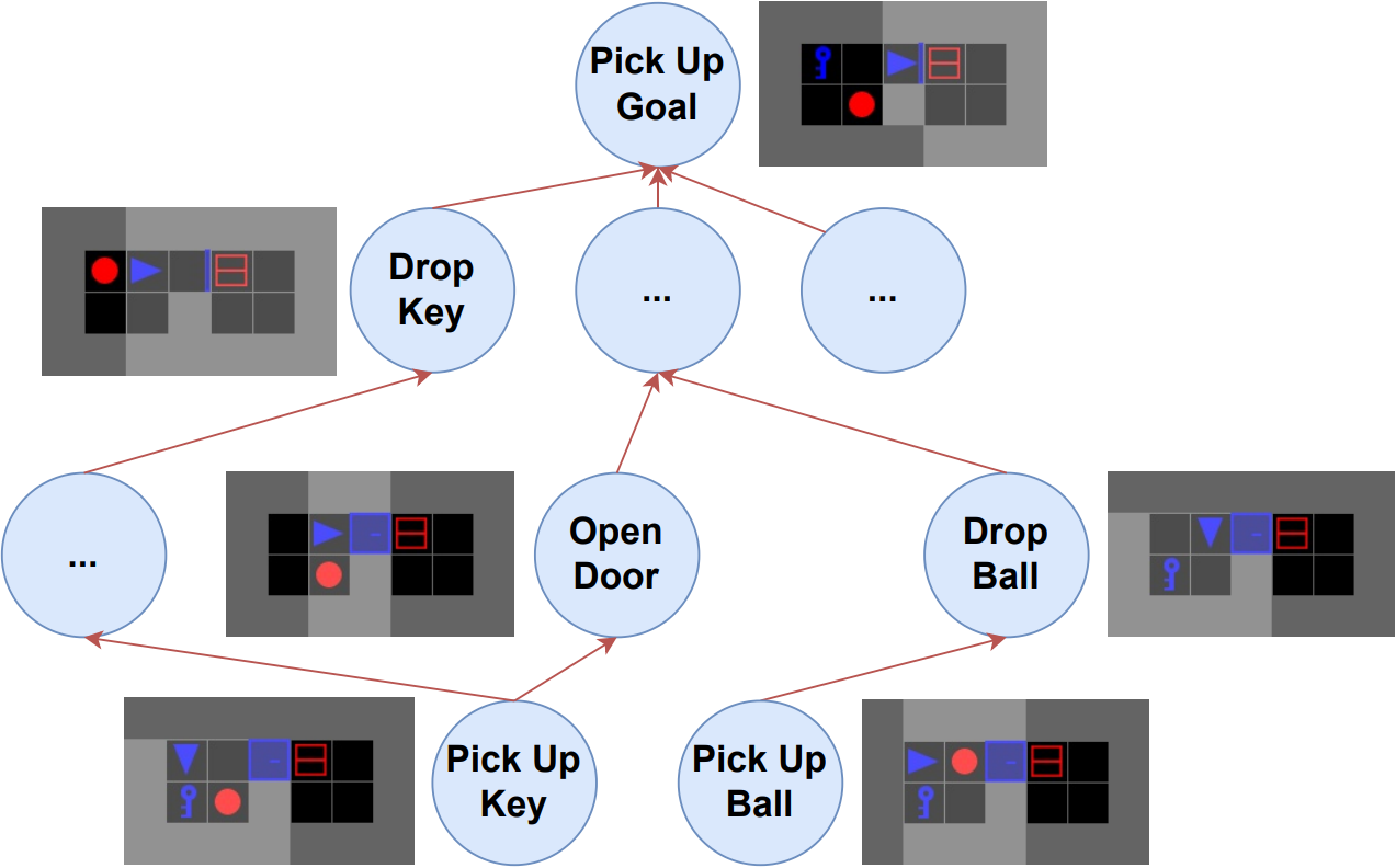
Causal Structure Discovery Contribution: We study the contribution of Phase 2, comparing between causality and attention correlation. We directly used the assigned to each in Phase 1 to compute the intrinsic reward: , where is the hyperparameter in Eq. 5. This reward differs from the ATTENTION reward used in Sect. 4.1 in that the augmentation in Eq. 6 is not applied. We expect that as attention score is a reliable indicator of correlation, building intrinsic reward upon it would benefit the agent, albeit not as effectively as when a causal graph is used (correlation is not as good as causality). The learning curve in Fig. 3(c) showcases that the result using causal as intrinsic motivation (green curve) performs better than using attention correlation (purple curve) by a large margin. To further evaluate, we extract the learned causal graph in Fig. 5 and present the detailed analysis of this graph in Supp. B. The result shows that our method can recover an approximation of the ground truth causal graph. Although there are redundant nodes and edges, important causal hierarchy is maintained, e.g., “open door” is the parental step of “pickup key”.
5 Conclusion
This paper introduces VACERL, a framework that enhances RL agent performance by analyzing causal relationships among agent observations and actions. Unlike previous methods, VACERL addresses causal discovery without assuming specified causal variables, making it applicable to variable-agnostic environments. Understanding these causal relationships becomes crucial for effective agent exploration, particularly in environments with complex causal structures or irrelevant actions, such as the Noisy-TV problem. We propose two methods to leverage the identified causal structure. Future research could explore other methods utilizing this structure. Empirical evaluations in sparse reward navigation and robotic tasks demonstrate the superiority of our approach over baselines. However, a limitation is the introduction of new hyperparameters, which require adjustment for different settings.
References
- [1] Andrychowicz, M., Wolski, F., Ray, A., Schneider, J., Fong, R., Welinder, P., McGrew, B., Tobin, J., Pieter Abbeel, O., Zaremba, W.: Hindsight experience replay. Advances in neural information processing systems 30 (2017)
- [2] Bellemare, M., Srinivasan, S., Ostrovski, G., Schaul, T., Saxton, D., Munos, R.: Unifying count-based exploration and intrinsic motivation. Advances in neural information processing systems 29 (2016)
- [3] Burda, Y., Edwards, H., Storkey, A., Klimov, O.: Exploration by random network distillation. arXiv preprint arXiv:1810.12894 (2018)
- [4] Chevalier-Boisvert, M., Dai, B., Towers, M., de Lazcano, R., Willems, L., Lahlou, S., Pal, S., Castro, P.S., Terry, J.: Minigrid & miniworld: Modular & customizable reinforcement learning environments for goal-oriented tasks. CoRR abs/2306.13831 (2023)
- [5] Corcoll, O., Vicente, R.: Disentangling causal effects for hierarchical reinforcement learning. arXiv preprint arXiv:2010.01351 (2020)
- [6] De Haan, P., Jayaraman, D., Levine, S.: Causal confusion in imitation learning. Advances in neural information processing systems 32 (2019)
- [7] Ding, W., Lin, H., Li, B., Zhao, D.: Generalizing goal-conditioned reinforcement learning with variational causal reasoning. Advances in Neural Information Processing Systems 35, 26532–26548 (2022)
- [8] Hu, X., Zhang, R., Tang, K., Guo, J., Yi, Q., Chen, R., Du, Z., Li, L., Guo, Q., Chen, Y., et al.: Causality-driven hierarchical structure discovery for reinforcement learning. Advances in Neural Information Processing Systems 35, 20064–20076 (2022)
- [9] Hung, C.C., Lillicrap, T., Abramson, J., Wu, Y., Mirza, M., Carnevale, F., Ahuja, A., Wayne, G.: Optimizing agent behavior over long time scales by transporting value. Nature communications 10(1), 5223 (2019)
- [10] Ke, N.R., Bilaniuk, O., Goyal, A., Bauer, S., Larochelle, H., Schölkopf, B., Mozer, M.C., Pal, C., Bengio, Y.: Learning neural causal models from unknown interventions. arXiv preprint arXiv:1910.01075 (2019)
- [11] de Lazcano, R., Andreas, K., Tai, J.J., Lee, S.R., Terry, J.: Gymnasium robotics (2023), http://github.com/Farama-Foundation/Gymnasium-Robotics
- [12] Le, H., Do, K., Nguyen, D., Venkatesh, S.: Beyond surprise: Improving exploration through surprise novelty. In: Proceedings of the 23rd International Conference on Autonomous Agents and Multiagent Systems. p. 1084–1092. AAMAS ’24, International Foundation for Autonomous Agents and Multiagent Systems, Richland, SC (2024)
- [13] Levy, A., Konidaris, G., Platt, R., Saenko, K.: Learning multi-level hierarchies with hindsight. arXiv preprint arXiv:1712.00948 (2017)
- [14] Lillicrap, T.P., Hunt, J.J., Pritzel, A., Heess, N., Erez, T., Tassa, Y., Silver, D., Wierstra, D.: Continuous control with deep reinforcement learning. arXiv preprint arXiv:1509.02971 (2015)
- [15] Mnih, V., Kavukcuoglu, K., Silver, D., Rusu, A.A., Veness, J., Bellemare, M.G., Graves, A., Riedmiller, M., Fidjeland, A.K., Ostrovski, G., et al.: Human-level control through deep reinforcement learning. nature 518(7540), 529–533 (2015)
- [16] Pearl, J.: Causal inference in statistics: An overview (2009)
- [17] Pitis, S., Chan, H., Zhao, S., Stadie, B., Ba, J.: Maximum entropy gain exploration for long horizon multi-goal reinforcement learning. In: International Conference on Machine Learning. pp. 7750–7761. PMLR (2020)
- [18] Pitis, S., Creager, E., Garg, A.: Counterfactual data augmentation using locally factored dynamics. Advances in Neural Information Processing Systems 33, 3976–3990 (2020)
- [19] Plappert, M., Andrychowicz, M., Ray, A., McGrew, B., Baker, B., Powell, G., Schneider, J., Tobin, J., Chociej, M., Welinder, P., et al.: Multi-goal reinforcement learning: Challenging robotics environments and request for research. arXiv preprint arXiv:1802.09464 (2018)
- [20] Samvelyan, M., Kirk, R., Kurin, V., Parker-Holder, J., Jiang, M., Hambro, E., Petroni, F., Kuttler, H., Grefenstette, E., Rocktäschel, T.: Minihack the planet: A sandbox for open-ended reinforcement learning research. In: Thirty-fifth Conference on Neural Information Processing Systems Datasets and Benchmarks Track (Round 1) (2021), https://openreview.net/forum?id=skFwlyefkWJ
- [21] Schulman, J., Wolski, F., Dhariwal, P., Radford, A., Klimov, O.: Proximal policy optimization algorithms. arXiv preprint arXiv:1707.06347 (2017)
- [22] Seitzer, M., Schölkopf, B., Martius, G.: Causal influence detection for improving efficiency in reinforcement learning. Advances in Neural Information Processing Systems 34, 22905–22918 (2021)
- [23] Silver, D., Schrittwieser, J., Simonyan, K., Antonoglou, I., Huang, A., Guez, A., Hubert, T., Baker, L., Lai, M., Bolton, A., et al.: Mastering the game of go without human knowledge. nature 550(7676), 354–359 (2017)
- [24] Sun, Z., He, B., Liu, J., Chen, X., Ma, C., Zhang, S.: Offline imitation learning with variational counterfactual reasoning. Advances in Neural Information Processing Systems 36 (2023)
- [25] Sutton, R.S., Barto, A.G.: Reinforcement learning: An introduction. MIT press (2018)
- [26] Tang, H., Houthooft, R., Foote, D., Stooke, A., Xi Chen, O., Duan, Y., Schulman, J., DeTurck, F., Abbeel, P.: # exploration: A study of count-based exploration for deep reinforcement learning. Advances in neural information processing systems 30 (2017)
- [27] Towers, M., Terry, J.K., Kwiatkowski, A., Balis, J.U., Cola, G.d., Deleu, T., Goulão, M., Kallinteris, A., KG, A., Krimmel, M., Perez-Vicente, R., Pierré, A., Schulhoff, S., Tai, J.J., Shen, A.T.J., Younis, O.G.: Gymnasium (Mar 2023). https://doi.org/10.5281/zenodo.8127026, https://zenodo.org/record/8127025
- [28] Vaswani, A., Shazeer, N., Parmar, N., Uszkoreit, J., Jones, L., Gomez, A.N., Kaiser, Ł., Polosukhin, I.: Attention is all you need. Advances in neural information processing systems 30 (2017)
- [29] Zeng, Y., Cai, R., Sun, F., Huang, L., Hao, Z.: A survey on causal reinforcement learning. arXiv preprint arXiv:2302.05209 (2023)
- [30] Zhang, P., Liu, F., Chen, Z., Jianye, H., Wang, J.: Deep reinforcement learning with causality-based intrinsic reward (2020)
- [31] Zhang, T., Guo, S., Tan, T., Hu, X., Chen, F.: Generating adjacency-constrained subgoals in hierarchical reinforcement learning. Advances in Neural Information Processing Systems 33, 21579–21590 (2020)
- [32] Zhang, Y., Du, Y., Huang, B., Wang, Z., Wang, J., Fang, M., Pechenizkiy, M.: Interpretable reward redistribution in reinforcement learning: A causal approach. Advances in Neural Information Processing Systems 36 (2024)
- [33] Todorov, E., Erez, T., Tassa, Y.: Mujoco: A physics engine for model-based control. In: 2012 IEEE/RSJ international conference on intelligent robots and systems. pp. 5026–5033. IEEE (2012)
A Details of Methodology
A.1 VACERL Framework
The detailed processing flow of the VACERL framework is described in Algo. 1. Buffer is initialized using the process from lines 2-6, using a random policy to collect successful trajectories (Note: as long as the agent can accidentally reach the goal and add 1 trajectory to , we can start the improving process). We, then, start our iterative process (the outer loop). In Phase 1, “Crucial Step Detection” (lines 8-21), the process commences with the training of the Transformer model using Algo. 2. Subsequently, we collect the dictionary that maps to attention score . is sorted based on . We, then, define function (line 9) and abstract function (line 10) to handle similar observation-action steps, and add the top steps to the set using the process from lines 12-20. After collecting , we apply Eq. 1 to acquire the new buffer . With buffer , we initiate Phase 2 (line 22) called “Causal Structure Discovery”. We optimize the two parameters and using Algo. 3 and collect the causal graph . Using graph , we collect the causal tree relative to the goal-reaching step to create a hierarchy of steps. We use this hierarchy to calculate the intrinsic reward associated with using Eq. 6 or to calculate subgoals sampling probability using Eq. 7. Finally, we train the policy and adding new successful trajectories to buffer , summarizing Phase 3 (lines 23-29) called “Agent Training with Causal Information”. The process starts again from Phase 1 using the updated buffer .
A.2 Transformer Model Training
Detailed pseudocode for training the Transformer model is provided in Algo. 2. We utilize the Transformer architecture implemented in PyTorch 222https://pytorch.org/docs/stable/generated/torch.nn.Transformer.html, for our model implementation. This implementation follows the architecture presented in the paper [28], thus, the attention score for a step is computed using the self-attention equation: , where represents the query vector, represents the key vector, is the learned embedding of a step , and are trainable weights. The values of are extracted from the encoder layer of the model during the last training iteration. We use a step as the key in dictionary that maps to an associated , described in the process in lines 5-11 (Algo. 2).
A.3 SCM Training
The detailed pseudocode is provided in Algo. 3. Our approach involves a two-phase iterative update process, inspired by the causal learning method proposed by Ke et al., [10]. This process optimizes two parameters: the functional parameter of generating function and the structural parameter of graph , representing a Structural Causal Model (SCM). In Phase 1 of the process, we want to keep the structural parameter fixed and update the functional parameter , whereas in Phase 2, we keep fixed and update . Both sets of parameters underwent training using the buffer (Eq. 1). The generating function is initialized as a 3-layer MLP neural network with random parameter . The parameter , the soft adjacency matrix of size representing the direct causality graph of the steps, is initialized as a random tensor, such that denotes the causal relationship between step at index of on step at index of . At each step in lines 4 and 20 of Algo. 3, we sample a hypothesis causal graph by Bernoulli sampling that will be used for the optimization process, where .
The intuition behind this optimization process is that the step representing the "cause" should occur before its associated "effect" step, so, for a step in the trajectory -th, we formulate as:
In our implementation, every steps from to that do not belong to the parental set of are masked out when inputting into the MLP, in this way, only steps that belong to the parental set of are used in the prediction of To learn and optimize parameter , we compute an MSE loss as denoted in Eq. 3.
In the second phase, we fix and optimize the parameter by updating the causality from variable to . After updating parameter for several steps, we return to the optimization process of parameter .
Finally, we use the resulting structural parameter to construct the final causal graph . We first get edge using Eq. 4, where, represents the causal confident threshold. In our implementation, was tuned with the values in . This Eq. 4 is used to ensure that there is no internal loop in the adjacency matrix.
A.4 Causal Tree Extraction
We extract a tree from the resultant causal graph , focusing on the steps relevant to achieving the goal. We use the goal-reaching step as the root of the tree and recursively determine the parental steps of this root node within graph and add them to the causal tree as new nodes, and subsequently, we will determine the parental steps for all these identified nodes. However, to avoid cycles in the tree, we need to add an order of ranking, thus, we use the ranking of attention score . So, for edge from variable to variable , we will remove the edge if of is smaller than the of , even if =1 according to the graph .
B Setting to Test VACERL Causal Intrinsic Reward
B.1 Environments
FrozenLake Environments
These tasks involve navigating the FrozenLake environments of both 4x4 (4x4FL) and 8x8 (8x8FL) [27]. Visualizations for these environments can be found in Fig. B.1(d,e). The goal of the agent involves crossing a frozen lake from the starting point located at the top-left corner of the map to the goal position located at the bottom-right corner of the map without falling into the frozen lake. The observation in these environments is a value representing the current position of the agent. The number of possible positions depends on the map size, with 4x4FL having 16 positions and 8x8FL having 64 positions. The agent is equipped with four discrete actions determining the direction of the agent’s movement [27]. If the agent successfully reaches the goal, it receives a +1 reward. However, if it falls into the lake or fails to reach the goal within a predefined maximum number of steps, it receives a 0 reward. The chosen maximum number of steps for 4x4FL and 8x8FL to validate our framework are 100 steps and 2000 steps, respectively.
Minihack Environments
These tasks involve MH-1 (MiniHack-Room-5x5-v0), MH-2 (MiniHack-Room-Monster-5x5-v0), MH-3 (MiniHack-Room-Ultimate-5x5-v0) and MH-4 (MiniHack-River-Narrow-v0); a suit of environments collected from [20]. These environments present more challenging exploration scenarios compared to FrozenLake environments due to the increased number of objects. Certain environments necessitate interaction with objects to achieve the goal, such as defeating monsters (MH-2 and MH-3) or constructing bridges (MH-4). If the agent successfully reaches the goal within a predefined maximum number of steps, it receives a +1 reward; otherwise, it receives a 0 reward. The maximum number of steps for all four environments is the default number of steps in [20].
Minigrid Environments
These tasks involve four environments: Key Corridor (MG-1 Fig. B.1(a)), two 2x2 rooms (MG-2 Fig. 1), two 3x3 rooms (MG-3 Fig. B.1(b)) and three 2x2 rooms (MG-4 Fig. B.1(c)). The goal of the agent, in MG-1, is to move and pick up the yellow ball and, in MG-2, MG-3 and MG-4, is to pick up a blue box which is located in the rightmost room, behind a locked door [4]. In these environments, the agent has six actions: turn left (L), right (R), move forward (F), pick up (PU), drop (D) and use (T) the object. With each new random seed, a new map is generated, including the agent’s initial position and the position of the objects. For MG-2, MG-3, and MG-4, there will always be an object obstructing the door. Specifically, for MG-3 and MG-4, the agent has to pick up a key with a matching colour to the door. In MG-3, we also introduce two distracted objects (the red ball and the green key in Fig. B.1(b)). All 3 environments are POMDP, meaning that the agent can only observe part of the map; the observation is an image tensor of shape [7,7,3]. The agent is equipped with six actions. Successfully reaching the goal within a predefined maximum number of steps results in a +1 reward for the agent; otherwise, it receives a 0 reward. The selected maximum number of steps for MG-1 is 270, MG-2 is 500, MG-3 is 1000 and for MG-4 is 5000. To complete these environments, the agent has to learn to move the ball by picking it up and dropping it in another location, then, it has to pick up the key, open the door and pick up the object in the other room.
B.2 Baseline Implementations
The backbone algorithm is Proximal Policy Optimization (PPO). We use the Pytorch implementation of this algorithm on the open-library Stable Baselines 3 333https://github.com/DLR-RM/stable-baselines3. To enhance the performance of this backbone algorithm, we fine-tuned the entropy coefficient and settled on a value of 0.001 after experimenting with [0.001, 0.005, 0.01, 0.05]. All other parameters were maintained as per the original repository. Subsequently, we incorporated various intrinsic reward baselines on top of the PPO backbone, including Count-Based, Random Network Distillation (RND), ATTENTION, CAI, and our VACERL.
For the Count-Based method, similar to the work of Bellemare et al. [2], we tracked the frequency of observations and associated actions and used the Simhash function to merge similar pairs [26]. The intrinsic reward is formulated as , where represents the count and is the simhash function. We tune the exploration bonus hyperparameter , however, there are no significant performance gains, as long as the bonus rewards do not overtake the rewards of the environment. Finally, we settle for a value of . We also test different values of the hashing parameters of the Simhash function. The final implementation used , which shows the best results and is consistent with the referenced paper [2].
We also adopt a public code repository for the implementation of RND (MIT License)444https://github.com/jcwleo/random-network-distillation-pytorch. To align the implementation with our specific environments, we have made adjustments to the input shapes and modified the PPO hyperparameters to match those of other baselines. We adhered to the implementation provided in the code, using the hyperparameter values as specified.
In the case of ATTENTION, we leveraged the attention scores from the encoder layer of the Transformer model as the reward signal. This approach has been used in the work of Pitis et al., [18] as a method to measure causal influence. The intrinsic reward has the form . We integrate this as an iterative process similar to our VACERL framework and also aid the exploration in the earlier phase using Eq. 6 for fairness. Similar to our framework VACERL and the implementation of Count-based, we use an value of for this baseline.
Finally, for the CAI method, we measure the causal influence between each observation-action pair with the observation-action pair of the goal-reaching step [22]. This is slightly different from the implementation of the original paper, which assumes the knowledge of the location of the goal and other objects. Our final implementation used a two-layer MLP neural network to measure CAI and it is based on the code of the original paper (MIT License)555https://github.com/martius-lab/cid-in-rl).
Additional details of hyperparameters can be found in Sec. D.
B.3 Additional Experiment Results
This section presents additional experiment results and visualization.
Learning Curve
The learning curves for the 4x4FL and 8x8FL tasks are illustrated in Fig. B.2; the learning curves for the MH-1 to MH-4 are illustrated in Fig. B.3, while the corresponding curves for MG-1, MG-3 and MG-4 are presented in Fig. B.5. The learning curves of VACERL in these figures show a similar pattern to the learning curves for MG-2 as presented in Fig. 2. Initially, the learning progress is slightly slower, as a number of training steps are required to acquire a correct causal representation. Subsequently, the performance accelerates rapidly, eventually surpassing baselines and attaining the optimal point.
The steps shown in these figures are the number of times the agent interacts with the environment, so for fairness, the number of steps of VACERL and causal baselines (CAI and ATTENTION) are computed as , where is the number of outer-loop iterations in line 7 of Algo. 1.
4x4FL Heatmap
The attention heatmap for the 4x4FL task is provided in Fig. B.6. These two figures show a similar pattern as in Fig. 4(a,b). Specifically, when the size of buffer B is small (Fig. B.6(a)), the accuracy of crucial step detection is not as precise compared to scenarios where the size of buffer B is larger (Fig. B.6(b)).
MG-2 Generated Causal Graph
The causal graph generated, as a result of our framework, for the MG-2 task is provided in Fig. 5. Each observation-action is associated with an image representing the map at the timestep that the agent executes the action. Below is a summary of the relationships and our rationale for why the agent generated the unexpected, though reasonable, relationship. Expected relationships:
-
•
Drop Key to Pick Up Goal.
-
•
Open Door to Pick Up Goal.
-
•
Pick Up Key to Drop Key.
-
•
Pick Up Key to Open Door.
-
•
Pick Up Ball to Drop Ball.
Unexpected Relationships:
-
•
Drop Ball to Pick Up Goal and not to Open Door: We believe that this unexpected relationship is because the agent is allowed to repeat action that it has taken before in the environment. Consequently, the agent can pick up the ball again after it opens the door, thus affect the relationship between Drop Ball and Open Door. In addition, as the agent can only hold one item at a time, it must drop the ball before picking up the goal, which creates a relationship between Drop Ball and Pick Up Goal. If this sequence of steps frequently occurs in collected trajectories, the agent will infer that this sequence represents an accurate relationship, thus leading to the generation of this causal graph. Although this relationship is not what we expected, the relationship is not inaccurate, particularly in this environment wherein the agent can only hold a single item at a time.
C Setting to Test VACERL with Causal Subgoal for HRL
C.1 Environments
Both of the environments used in this section are available in Gymnasium-Robotics [11] and are built on top of the MuJoCo simulator [33]. The robot in question has 7 degrees of freedom (DoF) and a two-fingered parallel gripper. In FetchReach, the state space is , and in FetchPickAndPlace, the state space is In both environments, the action space is , including actions to move the gripper and opening/closing of the gripper. In FetchReach, the task is to move the gripper to a specific position within the robot’s workspace, which is relatively simpler compared to FetchPickAndPlace. In the latter, the robot must grasp an object and relocate it.
In both cases, user are given two values which are “achieved_goal” and “desired_goal”. Here, "achieved_goal" denotes the final position of the object, and "desired_goal" is the target to be reached. In FetchReach, these goals represent the gripper’s position since the aim is to relocate it. While in FetchPickAndPlace, they signify the block’s position that the robot needs to manipulate. Success is achieved when the Euclidean distance between "achieved_goal" and "desired_goal" is less than .
Sparse rewards are employed in our experiments, wherein the agent receives a reward of if the goal is not reached and if it is. The maximum number of timesteps allowed in these environments is set to 100.
C.2 Baseline Implementations
We utilize the PyTorch implementation of DDPG+HER from the Stable Baselines 3 666https://github.com/DLR-RM/stable-baselines3 open-library as one of our baselines. The hyperparameters for this algorithm are set to benchmark values available in RL-Zoo 777https://github.com/DLR-RM/rl-baselines3-zoo. We assess the performance of this baseline against the results presented in the original robotic paper by Plappert et al. [19], noting similarities despite differences in environment versions.
For our HAC implementation, the core algorithm of our approach, we adopt a publicly available code repository 888https://github.com/andrew-j-levy/Hierarchical-Actor-Critc-HAC- (MIT License) by the author of the original paper [13]. We modify this code to align with our environments, where the goal position and the goal condition are supplied by the environments themselves. The baseline is implemented as a three-level DDPG+HER, in which the top two levels are used to supplied subgoals and the lowest level is used to learn the actions. We adjust the hyperparameters of the lowest level DDPG+HER to match those of the DDPG+HER baseline for fairness.
Additional details of hyperparameters can be found in Sec. D.
C.3 Additional Experiment Results
 |
 |
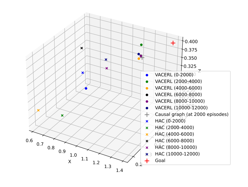
To validate our assertion that causal subgoals can effectively narrow down the search space for an HRL agent to significant subgoals, thus enhancing HRL sample efficiency in Robotic-Environments, we present an additional experiment along with the visualization of subgoals’ average coordinates selected by VACERL and Vanilla HAC in this experiment (Fig. C.1). The experiment was conducted in the FetchReach environment, with the causal graph re-evaluated every 2,000 steps, mirroring our main experiments. We specifically chose a run where initial subgoals of HAC and VACERL exhibited similar average coordinates (x, y, z) for fairness. In this run, the goal (indicated by a red + marker) was positioned at coordinates (1.38294353, 0.68003652, 0.396999).
As illustrated in Fig. C.1(a), despite the initial subgoals’ average coordinates being very similar (represented by blue markers) – (0.727372811, 0.501121846, 0.28868408) for HAC and (0.7377534, 0.521795303, 0.2345436) for VACERL – VACERL swiftly converges to subgoals much closer to the goal after just one iteration of causal discovery learning, while, Vanilla HAC struggles to converge. We plot the weighted average coordinates of nodes in the causal graph after this iteration (indicated by a grey + marker), with weights determined by the probability of node sampling according to Eq. 7; higher probabilities correspond to higher weights. We choose to plot the values of this iteration because it represents the instance where VACERL undergoes the most significant shift in subgoals’ coordinates. The results indicate that the coordinates of nodes in the causal graph closely align with the coordinates of subgoals sampled by the top-level policy. This supports our intuition that causal subgoals contribute to the improvement in subgoal sampling and the overall sample efficiency of HRL.
The improvement is also reflected in the associated learning curve, in Fig. C.1(b), of the agent: after training for 4,000 episodes, VACERL begins to learn the environment, whereas HAC requires 8,000 episodes – coinciding with the point where the agent starts selecting subgoals with coordinates closer to the goal.
D Architecture and Hyperparameters of VACERL
The default hyperparameters (if not specified in accompanying tables then these values were used) are provided in Table. 2. The definitions and values for hyperparameters, which require tuning and may vary across different environments, are specified in the accompanying tables. The system’s architecture and the explanation for tuning of hyperparameter are outlined below:
Architecture
-
•
model’s architecture: , , , .
-
•
Functional model ’s architecture: 3-layer MLP, .
-
•
PPO: Stable Baselines 3’s hyperparameters with entropy coefficient
-
•
DDPG+HER: RL-Zoo’s architecture and hyperparameters for FetchReach and FetchPickAndPlace environments.
-
•
HAC: 3-levels DDPG+HER, architectures and hyperparameters are the same with DDPG+HER.
Tuning
-
•
(used for VACERL and all causal baselines): This hyperparameter requires tuning as it relies on the complexity of the environment. The more challenging the environment, the greater the number of head steps required to gather a successful trajectory and start the framework. For MG, FL, and MH environments, we use a random policy to collect this initial phase, however, in challenging robotic environments where collecting successful trajectories is difficult, we leverage the underlying HAC agent to gather these trajectories. Consequently, the value of equals in such environments. Additionally, in MG, FL, and MH denotes the number of time the agent interacts with the environments, whereas in robotic environments, it denotes episode.
-
•
: This hyperparameter requires tuning as it depends on the state-space of the environment. Generally, a larger state-space requires a larger value for . However, as shown in Fig. 4, too large can introduce noise during the causal structure discovery phase and affect the final policy training result.
-
•
: This hyperparameter is only used in continuous space environments.
-
•
(used for VACERL and all causal baselines): Similar to , this hyperparameter varies between environments. in MG, FL, and MH denotes the number of steps the agent interacts with the environments, whereas in robotic environments, it denotes episode. is also the number of steps/episodes before the causal graph is reconstructed.
| Hyperparameters | Def. | Value |
|---|---|---|
| Learning rate of model | ||
| Learning rate of parameter | ||
| Learning rate of parameter | ||
| No. iteration causal discovery | ||
| Training steps for functional parameter | ||
| Training steps for structural parameter | ||
| Causality threshold in Eq. 4 | ||
| Intrinsic Coef. |
| Hyperparameters | Def. | 4x4FL | 8x8FL |
|---|---|---|---|
| Head steps to start the framework | |||
| Number of top attention steps | |||
| Similary threshold in function. | - | - | |
| Training steps of policy |
| Hyperparameters | Def. | MH-1 | MH-2 | MH-3 | MH-4 |
|---|---|---|---|---|---|
| Head steps to start the framework | |||||
| Number of top attention steps | |||||
| Similary threshold in function. | |||||
| Causality threshold in Eq. 4 | |||||
| Training steps of policy |
| Hyperparameters | Def. | MG-1 | MG-2 | MG-3 | MG-4 |
|---|---|---|---|---|---|
| Head steps to start the framework | |||||
| Number of top attention steps | |||||
| Similary threshold in function. | |||||
| Training steps of policy |
| Hyperparameters | Def. | FETCHPUSH | FETCHPICKANDPLACE |
|---|---|---|---|
| Head episodes to start the framework | |||
| Number of top attention steps | |||
| Similary threshold in function. | |||
| Causality threshold in Eq. 4 | |||
| Training steps of policy |