Validation of the static forward Grad–Shafranov equilibrium solvers in FreeGSNKE and Fiesta using EFIT++ reconstructions from MAST-U

Abstract

Abstract. A key aspect in the modelling of magnetohydrodynamic (MHD) equilibria in tokamak devices is having access to fast, accurate, and stable numerical simulation methods. There is an increasing demand for reliable methods that can be used to develop traditional or machine learning-based shape control feedback systems, optimise scenario designs, and integrate with other plasma edge or transport modelling codes. To handle such applications, these codes need to be flexible and, more importantly, they need to have been validated against both analytically known and real-world tokamak equilibria to ensure they are consistent and credible. In this paper, we are interested in solving the static forward Grad–Shafranov (GS) problem for free-boundary MHD equilibria. Our focus is on the validation of the static forward solver in the Python-based equilibrium code FreeGSNKE by solving equilibria from magnetics-only EFIT++ reconstructions of MAST-U shots. In addition, we also validate FreeGSNKE against equilibria simulated using the well-established MATLAB-based equilibrium code Fiesta. To do this, we develop a computational pipeline that allows one to load the same (a)symmetric MAST-U machine description into each solver, specify the required inputs (active/passive conductor currents, plasma profiles and coefficients, etc.) from EFIT++, and solve the GS equation for all available time slices across a shot. For a number of different MAST-U shots, we demonstrate that both FreeGSNKE and Fiesta can successfully reproduce various poloidal flux quantities and shape targets (e.g. midplane radii, magnetic axes, separatrices, X-points, and strikepoints) in agreement with EFIT++ calculations to a very high degree of accuracy. We also provide public access to the code/data required to load the MAST-U machine description in FreeGSNKE/Fiesta and reproduce the equilibria in the shots shown.

Keywords. MHD equilibria $\bullet$ Grad–Shafranov $\bullet$ FreeGSNKE $\bullet$ Fiesta $\bullet$ EFIT++ $\bullet$ MAST-U

UKAEAUnited Kingdom Atomic Energy Authority, Culham Campus, Abingdon, Oxfordshire, OX14 3DB, United Kingdom
() HartreeSTFC Hartree Centre, Sci-Tech Daresbury, Keckwick Lane, Daresbury, Warrington, WA4 4AD, United Kingdom

1 Introduction

Developing fast and accurate numerical methods for simulating the magnetohydrodynamic (MHD) equilibrium of a magnetically-confined plasma is a crucial element in the design and operation of existing and future tokamak devices. These methods are used extensively to analyse different plasma scenarios, shapes, and stability, in addition to playing a critical role in the operation and optimisation of control and real-time feedback systems.

In this paper, we focus on the free-boundary static forward MHD equilibrium problem, which involves solving the Grad–Shafranov (GS) equation for a toroidally symmetric, isotropic plasma equilibrium—see Section 3 for further details. A vast array of numerical codes exist for solving this problem, however, our focus will be on two in particular: FreeGSNKE and Fiesta (more details to follow in Section 2). The aim of this work is to:

1. validate that the static forward solver in FreeGSNKE can reproduce the equilibria obtained by a magnetics-only EFIT++ reconstruction on the MAST-U tokamak (in addition to those produced by Fiesta).

2. compare poloidal flux quantities, shape control measures (e.g. midplane radii, magnetic axes, and separatrix positions), and other targets (e.g. X-points and strikepoints) from both solvers for a number of physically different MAST-U shots, using EFIT++ as the reference solution.

To enable an accurate and valid comparison of the results, we need to ensure that both FreeGSNKE and Fiesta are set up using the same set of input quantities as used by EFIT++. Firstly, this will require a consistent description of the MAST-U machine that includes the active coils, passive structures, and the wall/limiter. We require details of their positions, orientations, windings, and polarity. Secondly, for each equilibrium, we need to appropriately assign values for both the active/passive conductor currents and plasma profiles parameters as calculated by EFIT++. In Section 4, we provide more details on these input quantities and highlight differences between each code implementation.

Carrying out robust validation of static GS solvers, against both analytic solutions and real-world tokamak plasmas, is critical for users that require consistent and reliable equilibrium calculations. We should stress that while the reference EFIT++ equilibria are obtained as equilibrium reconstructions, and are therefore the result of a fitting procedure from experimental measurements on the MAST-U tokamak, here we do not perform the same fitting procedure in FreeGSNKE or Fiesta. We instead use the coil currents and plasma profiles parameters fitted by EFIT++ as inputs to the static forward GS problems in FreeGSNKE and Fiesta. Given a consistent set of inputs across all codes, we will demonstrate that all three return quantitatively equivalent equilibria. By making the scripts required to do so publicly available, we hope to establish a common validation benchmark for other static forward GS equilibrium codes.

The rest of this paper will be structured as follows. In Section 2, we provide an introduction to the three solvers FreeGSNKE, Fiesta, and EFIT++, briefly discussing their capabilities and prior usage in different areas of tokamak equilibrium modelling. In Section 3, we outline the free-boundary static forward GS problem and note differences between the FreeGSNKE and Fiesta solution methods. Following this, we supply a more detailed description of the MAST-U machine and other more specific inputs required by each solver in Section 4.

In Section 5, we present our numerical experiments, focusing on two different MAST-U shots, one featuring a conventional divertor configuration and the other a Super-X (Morris et al., 2014, 2018). We begin by comparing FreeGSNKE and Fiesta, ensuring that we understand any key differences between the codes and how these differences may filter through when comparing with EFIT++. After this, we begin to assess the differences between equilibria (and other shape targets) from the solvers and those reconstructed from the diagnostics via EFIT++. We find excellent agreement between all quantities assessed and highlight the accuracy of both FreeGSNKE and Fiesta. Finally in Section 6, we discuss the implication of these results and close with a few suggestions for avenues of future work.

2 The solvers

In this section, we give a short introduction to the codes described in this paper and briefly discuss their capabilities.

2.1 FreeGSNKE

FreeGSNKE is a Python-based, finite difference, dynamic free-boundary toroidal plasma equilibrium solver developed by Amorisco et al. (2024) and built as an extension of the publicly available FreeGS code (Dudson, 2024). FreeGS features an inverse solver to perform static constrained equilibrium analyses, where user-specified controls (e.g. isoflux/X-point locations and coil currents) are used to determine a set of coil currents to achieve a desired equilibrium. This type of analysis is used in designing and controlling different types of plasma configurations prior to experimentation—a brief introduction to constrained analysis can be found in Jeon (2015)[Sec. II.7.]. FreeGS also features a static forward solver, where coil currents are instead fixed by the user and the corresponding plasma equilibrium is calculated. Both solvers in FreeGS use Picard iterations to solve the forward and inverse GS problems. They have been used, in conjunction with other equilibrium codes, extensively in recent years for the design of various tokamaks. To our knowledge, FreeGS has aided the design of SPARC (Creely et al., 2020), KSTAR (Lee et al., 2021), WEST (Maquet et al., 2023), Thailand Tokamak-1 (Sangaroon et al., 2023), and MANTA (MANTA Team, 2023). It was also used in the design of ARC (de Boucaud et al., 2022), with further work on DIII-D EFIT reconstructed equilibria, and to design COMPASS-U (Kripner et al., 2018), alongside Freebie (Artaud and Kim, 2012) and Fiesta, and to help develop the BLUEPRINT framework (Coleman and McIntosh, 2020).

FreeGSNKE inherits the FreeGS inverse solver and introduces an upgraded static forward solver, that uses a Newton–Krylov method (see e.g. Knoll and Keyes (2004); Carpanese (2021)), to overcome the well-known numerical instability affecting Picard iterations. Also introduced is a solver for the evolutive (dynamic) equilibrium problem, also based on the Newton–Krylov method. In the dynamic problem, Poynting’s theorem is enforced on the plasma, coupling the circuit equations (that govern currents in the active coils/passive structures) and the GS equation itself (Amorisco et al., 2024).

These features, as well as the widespread validation and use of the underlying FreeGS code, make FreeGSNKE a particularly versatile tool for studying the shape and control of plasma equilibria. Its compatibility with other Python libraries, especially those with machine learning capabilities, facilitate its future development and integration with other plasma modelling codes. For example, FreeGSNKE has been used to emulate scenario and control design in a MAST-U-like tokamak by Agnello et al. (2024), where their objective was to emulate flux quantities and shape targets (some of which we calculate here) based on a training library of input plasma profile parameters and active conductor currents.

The static forward solver in FreeGSNKE has been validated against analytic solutions of the GS equation and against the original iterative solver implemented in FreeGS (Amorisco et al., 2024). We now go a step further by implementing the full MAST-U machine description and validating the static solver against EFIT++ reconstructions.

2.2 Fiesta

Fiesta is a free-boundary static equilibrium solver written in MATLAB and developed by Cunningham (2013). In addition to being able to carry out forward and inverse equilibrium calculations, it is also capable of linearised dynamic modelling using the RZIp rigid plasma framework (Coutlis et al., 1999). It has been used to inform design choices and carry out equilibrium analyses on a number of tokamaks including JET, DIII-D, NSTX, TCV, MAST(-U) (Windridge et al., 2011; Cunningham, 2013), MEDUSA-CR (Araya-Solano et al., 2021), COMPASS-U (Vondracek et al., 2021), SMART (Doyle et al., 2021; Mancini et al., 2023), STEP (Hudoba et al., 2023), and EU-DEMO (Morris et al., 2021).

Having already been used to simulate MAST(-U) and other tokamak equilibria, we run Fiesta alongside FreeGSNKE to demonstrate they both return quantitatively equivalent equilibria given the same set of input data from EFIT++. This cross-validation process should also help identify and explain any differences between the two different implementations.

2.3 EFIT++

EFIT, first proposed by Lao et al. (1985), is a computational method that is widely used as a first port of call to “fit” (or reconstruct) the plasma equilibrium in a tokamak using diagnostic measurement data as constraints. These measurements come from diagnostics such as poloidal flux loops, pickup coils, Rogowski coils, motional Stark effect (MSE), and Thomson scattering systems, which are strategically located at key locations around the tokamak. Written in Fortran, EFIT it is used primarily for post-shot equilibrium reconstruction and has been implemented on a number of different tokamak devices (see below). Our focus is on EFIT++, a substantial re-write in which the original EFIT code has been wrapped in a C++ driver to handle data flow, which in turn is wrapped in a highly configurable Python layer for input and output checking. It is currently in use on the MAST-U tokamak (Appel et al., 2006) and was previously deployed on JET (Appel and Lupelli, 2018). We note that EFIT++ is run routinely for all MAST-U plasma shots using magnetic diagnostic data only and, if available, MSE data to improve the accuracy of core profiles. In addition to this, EFIT++ is also set up to use Thomson scattering data if required (Berkery et al., 2021; MAST Upgrade Team et al., 2022).

To solve the inverse problem, EFIT++ requires descriptions of the plasma pressure and toroidal current profiles which are typically expressed using basis functions (whose coefficients are to be adjusted during the fitting process). Next, the linearised GS equation is solved using an initial guess for the poloidal flux. The feasibility of the calculated flux with respect to the diagnostic measurement data is then measured by solving a linearised least-squares minimisation problem. During this process, the variable parameters such as the conductor currents and profile coefficients are adjusted to improve the fit. This iterative process repeats until the conductor currents, profile coefficients, and poloidal flux, together, return a valid solution to the GS equation at the required tolerance. For more technical details, refer to Lao et al. (2005), Appel and Lupelli (2018), and Bao et al. (2023).

Different versions of EFIT, each with their own configurations and modifications, have been used for equilibrium reconstruction on a vast array of tokamak devices. Without providing an exhaustive list, it has been deployed on JET (Appel and Lupelli, 2018), MAST(-U) (MAST Upgrade Team et al., 2022), EAST (Bao et al., 2023), DIII-D (Lao et al., 2005), START (Appel et al., 2001), KSTAR (Lee et al., 1999), NSTX (Sabbagh et al., 2001), and ITER (Lao et al., 2022). Given its history of widespread use on many different tokamak devices, we use EFIT++ as a source of trusted reference equilibria, against which to compare those produced by FreeGSNKE and Fiesta.

3 The static forward Grad–Shafranov problem

In this paper, we are interested in solving the Grad–Shafranov (GS) equation

$$\Delta^{*}\psi=-\mu_{0}R\underbrace{\left(J_{p}+J_{c}\right)}_{=J_{\phi}},\quad(R,Z)\in\Omega,$$ (3.1)

in the cylindrical coordinate system $(R,\phi,Z)$ for the poloidal flux $\psi(R,Z)$ (Grad and Rubin, 1958; Shafranov, 1958). Note here that $\mu_{0}$ represents magnetic permeability in a vacuum and $\Delta^{*}\coloneqq R\partial_{R}R^{-1}\partial_{R}+\partial_{ZZ}$ is a linear elliptic operator. The toroidal current density $J_{\phi}(\psi,R,Z)\coloneqq J_{p}(\psi,R,Z)+J_{c}(R,Z)$ contains a contribution from both the plasma $J_{p}$ and any toroidally symmetric conducting metal structures external to the plasma $J_{c}$ (e.g. active poloidal field coils and passive structures around the tokamak). The total poloidal flux $\psi\coloneqq\psi_{p}+\psi_{c}$ is also made up of a plasma $\psi_{p}$ and external conductor $\psi_{c}$ contribution. We wish to solve (3.1) over a two-dimensional computational domain $\Omega\coloneqq\Omega_{p}\cup\Omega_{p}^{\prime}$ where $\Omega_{p}$ represents the plasma region and $\Omega_{p}^{\prime}$ is its complement.

The plasma current density, non-zero only within the plasma region $\Omega_{p}$, takes the form

$$J_{p}(\psi,R,Z)=R\frac{\partial p}{\partial\psi}+\frac{1}{\mu_{0}R}F\frac{\partial F}{\partial\psi},\quad(R,Z)\in\Omega_{p},$$ (3.2)

where $p\coloneqq p(\psi)$ is the isotropic plasma pressure profile and $F\coloneqq F(\psi)=RB_{\phi}$ is the toroidal current profile ($B_{\phi}$ is the azimuthal component of the magnetic field). The particular choice of profile functions used in $J_{p}$ will be discussed in Section 4. The current density generated by $N_{c}$ external conductors is given by

$$J_{c}(R,Z) =\sum_{j=1}^{N_{c}}\frac{I_{j}^{c}(R,Z)}{A_{j}^{c}},\quad(R,Z)\in\Omega,$$ (3.3)

$$I_{j}^{c}(R,Z) =\begin{cases}I_{j}^{c}&\ \text{if}\ (R,Z)\in\Omega_{j}^{c},\vspace*{0.00cm}\\ 0&\ \text{elsewhere},\vspace*{0.00cm}\end{cases}$$

where $\Omega_{j}^{c}$, $I_{j}^{c}$, and $A_{j}^{c}$ are the domain region, current, and cross-sectional area of the $j$^th conductor, respectively. Note that external conductors can lie inside $\Omega$ as well as outside of it.

To complete the free-boundary problem, an appropriate Dirichlet boundary condition must also be specified on the domain boundary $\partial\Omega$—which we will now discuss. The dependence of $J_{p}$ on $\psi$ makes (3.1) a nonlinear elliptic partial differential equation.

3.1 Solving the problem

Here, we briefly outline the steps typically carried out when numerically solving the static free-boundary (forward) GS problem (Jardin, 2010; Jeon, 2015). For more specific details on how each of the solvers do this in practice, we refer the reader to the respective code documentation.

Before solving, we assume that a number of input parameters have already been provided by the user including: a machine (tokamak) description, conducting structure (active coil and passive structure) currents, and plasma profile functions (and parameters). More details on the specific inputs required for generating free-boundary equilibria on MAST-U with each of the codes will be described in Section 4.

Step one

Denote the total flux by $\psi^{(n)}(R,Z)$, where $n=0,1,\ldots$ is the iteration number, and generate an appropriate guess $\psi^{(0)}$ to initialise the solver.

Step two

Calculate the values of the flux on the computational boundary $\partial\Omega$ (i.e. the Dirichlet boundary condition) using

$$\psi^{(n)}\bigg{\rvert}_{\partial\Omega} =\int_{\Omega_{p}}G(R,Z;R^{\prime},Z^{\prime})J_{p}(\psi^{(n)},R^{\prime},Z^{\prime})\ \mathrm{d}R^{\prime}\mathrm{d}Z^{\prime}$$

$$+\sum_{j=1}^{N_{c}}\frac{1}{A_{j}^{c}}\int_{\Omega_{j}^{c}}G(R,Z;R^{\prime},Z^{\prime})I_{j}^{c}(R^{\prime},Z^{\prime})\ \mathrm{d}R^{\prime}\mathrm{d}Z^{\prime},$$ (3.4)

where the first and second terms are the contributions from $\psi^{(n)}_{p}$ and $\psi^{(n)}_{c}$ on the boundary, respectively. $G$ is a Green’s function for the operator $\Delta^{*}$ containing elliptic integrals of the first and second kind—it can be calculated by solving (3.1) with $\psi_{c}$ alone (see Jardin (2010)[Chp. 4.6.3]). To calculate (3.1), the plasma domain $\Omega_{p}$ (i.e. the area contained within the last closed flux surface) needs to be identified—see Jeon (2015)[Sec. 5] for how to do this. Once found, the integral itself can be calculated a number of different ways, for example, using von Hagenow’s method (Jardin, 2010)[Chp. 4.6.4].

Step three

To solve the nonlinear problem, both EFIT++ and Fiesta use Picard iterations (Kelley, 1995), where the $n$-th iteration consists of calculating the total flux $\psi^{(n+1)}$ according to

$$\Delta^{*}\psi^{(n+1)}=-\mu_{0}RJ_{\phi}(\psi^{(n)},R,Z),\quad(R,Z)\in\Omega,$$ (3.5)

together with boundary condition (3.1). In a finite difference implementation this requires spatially discretising the elliptic operator $\Delta^{*}$. For example, FreeGSNKE uses fourth-order accurate finite differences while Fiesta uses a second-order accurate (fast) discrete sine transform.

Step four

Check whether or not the solution meets a pre-specified tolerance, e.g. a relative difference such as

$$\frac{\max|\psi^{(n+1)}-\psi^{(n)}|}{\max(\psi^{(n)})-\min(\psi^{(n)})}<\varepsilon.$$ (3.6)

If so, we stop the iterations, otherwise we continue.

Both FreeGSNKE and Fiesta are set to use the same relative tolerance $\varepsilon=1\text{e}\mathord{-}6$ and while FreeGSNKE uses the criterion in (3.6), we should note that Fiesta uses a slightly different relative criterion based on values of $J_{p}$ at successive iterations instead of $\psi$. This should make little difference to the comparison.

Comments

Picard iterations are very effective at tackling inverse GS problems, which is the primary use case for EFIT++ and Fiesta. However, it is well-known that these iterations are unstable when applied to forward GS problems. This manifests itself in the form of vertically unstable equilbria that artificially move between successive Picard iterations (Carpanese, 2021). This arises as a result of a combination of known physical instabilities in highly-elongated plasmas and mathematical features of the Picard method itself (which stem from a combination of steep gradients in the nonlinear function and a poor initial guess to the solution). Newton-based methods can overcome this instability (see e.g. Carpanese (2021)). FreeGSNKE implements a Jacobian-free Newton–Krylov method (see Amorisco et al. (2024)[App. 1] for further details). This is used to solve directly for the roots, $\psi$, of

$$\Delta^{*}\psi+\mu_{0}RJ_{\phi}(\psi,R,Z)=0,\quad(R,Z)\in\Omega.$$ (3.7)

As with the Picard iteration, solving this problem still requires an appropriate initial guess and the calculation of the (nonlinear) boundary condition (3.1).

4 Input parameters (for MAST-U)

To solve the forward problem, we need to ensure that the inputs to both FreeGSNKE and Fiesta are consistent with those used by EFIT++ on MAST-U. We require:

1. an accurate and representative MAST-U machine description containing the:

   1. active poloidal field coils.

   2. passive structures.

   3. limiter/wall structure.

2. the fitted values of the coil currents of both active coil and passive structures.

3. the functional form chosen for the plasma profile functions and the corresponding fitted parameter values.

4. any additional parameters specific to either FreeGSNKE or Fiesta.

In the following sections, we outline how these inputs are configured for each of the codes .

4.1 Machine description

The following machine description had already been implemented in both EFIT++ and Fiesta and has now been set up in FreeGSNKE. We note here that numerical experiments (in Section 5) across all codes are simulated on a $65\times 65$ computational grid on $\Omega=[0.06,2.0]\times[-2.2,2.2]$, as this is the resolution EFIT++ is run at during MAST-U reconstructions.

4.1.1 Active coils

MAST-U contains 12 active poloidal field coils whose voltages can be varied for shaping and controlling the plasma (Ryan et al., 2023). In Figure 4.1, we display a poloidal cross-section of the machine (as is implemented in all three codes) with an example equilibrium from a MAST-U shot (all simulated and plotted using FreeGSNKE). The solenoid, named P1 on MAST-U, generates plasma current and a poloidal magnetic field while P4/P5/PC (the latter of which is not currently connected to the machine) are used for core radial position and shape control. P6 is used for core vertical control, D1/D2/D3/PX for X-point positioning and divertor leg control, and DP for further X-point positioning and flux expansion. Coils D5 and D6/D7 are used for Super-X leg radius and expansion control, respectively.

All active coils (except the solenoid) have an upper (labelled in Figure 4.1) and lower component (not labelled) that are wired together in the same circuit. All upper and lower coils are wired in series, except for the P6 coil, whose upper and lower components are connected in anti-series so that it can be used for vertical plasma control. Each coil consists of a number of filaments/windings (plotted as small blue rectangles on the right hand side of Figure 4.1) each with their own central position $(R,Z)$, width and height ($dR,dZ)$, polarity ($+1$ in series, $-1$ in anti-series), and current multiplier factor (used for the solenoid only). For the scope of the poloidal field, individual windings are modelled as infinitesimally thin toroidal filaments in both FreeGSNKE and Fiesta. Each filament also features its own resistivity value, however, this is not used here where we only deal with static equilibria.

We should note that when EFIT++ fits the active coil currents to diagnostic data, it does not treat the upper and lower windings of the same active coil as being linked in series. Instead, current values in the upper and lower windings are measured using independent Rogowski coils and are therefore fit to slightly different values. The relative difference between the upper/lower coil current values is very small and so using this configuration makes little difference to equilibria generated by EFIT++. We refer to this configuration as having non-symmetric (or up-down independent) coil currents. For both FreeGSNKE and Fiesta, we have the option to model the pairs of active coils as either symmetric (connected in series/anti-series as they are in the real MAST-U machine) or non-symmetric (as in EFIT++). All of the experiments presented in Section 5 are carried out using the non-symmetric coil setup so that we can recreate the EFIT++ configuration as closely as possible.

Figure 4.1: Left: Poloidal cross-section of the MAST-U machine (as used across all three codes) with FreeGSNKE-simulated equilibrium of shot $45292$ ($t=0.55$s). Shown are the 12 active coils (blue), the passive structures (dark grey), the limiter/wall (black line, white interior), and locations of shape targets to be tracked in experiments later on. Right: magnified view of the lower left corner of the machine (dark shaded box on left figure), showing individual filaments/windings inside some of the active coils and passive structures.

4.1.2 Passive structures

Both the active coils and the plasma itself induce significant eddy currents in the toroidally continuous conducting structures within MAST-U (McArdle and Taylor, 2008; Berkery et al., 2021). This is especially the case in spherical tokamak devices, due to the close proximity of passive structures to the plasma core and active coils. These currents significantly impact the plasma shape and position, making their inclusion in the modelling process essential to obtaining accurate equilibrium simulations.

The complete MAST-U machine description includes a total of 150 passive structures, making up the vessel, centre column, support structures, gas baffles, coil cases, etc. This number excludes a few structures that are not included in the EFIT++ model. These include the graphite tiles (which do not carry much current) and the cryopump (which contains a toroidal break to prevent large toroidal currents flowing around the machine). Each passive structure is represented by a parallelogram in the poloidal plane, defined by its central position $(R,Z)$, width and height $(dR,dZ)$ and two angles, $(\theta_{1},\theta_{2})$. Such parallelograms can be seen on the right hand side of Figure 4.1. Given that all three codes require these parallelogram structures to simulate equilibria in the $(R,Z)$ plane, we should note that this passive structure model is a reduced axisymmetric representation of the true three-dimensional MAST-U vessel which contains toroidal breaks for vessel ports among other things—see Berkery et al. (2021)[Fig. 12] for a depiction of the full 3D model.

Both FreeGSNKE and Fiesta model the poloidal field associated with each passive structure by uniformly distributing its current density over the poloidal cross-section. This can be done by “refining” (i.e. subdividing) each passive structure into individual filaments. We revisit this in Section 4.2 when we discuss how to assign currents to the passive structures.

4.1.3 Limiter/wall structure

The purpose of the limiter/wall in FreeGSNKE and Fiesta is to confine the boundary of the plasma. In all three codes it is described by 98 pairs of $(R,Z)$ coordinates that form the closed polygonal shape seen in Figure 4.1 (enclosing the flux contours). The plasma core is forced to reside within the limiter region, with the last closed flux surface being either fully contained in this region or tangent to its polygonal edge.

4.2 Assigning currents

4.2.1 Active coils

As mentioned before, both FreeGSNKE and Fiesta have the option to use symmetric or non-symmetric (independent) active coil current assignments. To set the coil currents in the non-symmetric setting, we assign the individually calculated upper/lower coil currents from EFIT++ directly to the corresponding coils in FreeGSNKE and Fiesta without modification. If we were to use the symmetric coil setting, however, each of the 12 active coils in FreeGSNKE and Fiesta require a single current value. To set each one, we could, for example, take the average of the corresponding upper and lower coil currents from EFIT++, making sure that the correct polarity of each current is also assigned.

4.2.2 Passive structures

Due to the different ways they are modelled in EFIT++, care needs to be taken when assigning the fitted passive structure currents to the 150 structures defined in Fiesta and FreeGSNKE. For example, current values for each coil case are fit by EFIT++ explicitly (using the Rogowski coil measurements mentioned before), which makes it easy to assign them directly in both FreeGSNKE and Fiesta. Other passive structure currents in the vessel, centre column, gas baffles, and support structures, are not, however, measured (and therefore fit) directly. To reduce the degrees of freedom in EFIT++, these passive structures are modelled in groups, each referring to a single current value, thereby reducing the computational runtime and avoiding some issues created by having too much freedom in the distribution of current around the machine (Berkery et al., 2021)[Sec. 3]. In total, in MAST-U there are 20 groups: 14 for the vacuum vessel, 2 for the gas baffles, 2 for passive stabilisation plates, and 2 for divertor coil supports (Kogan et al., 2021). To set the correct current for each structure in a group, we follow Berkery et al. (2021)[Sec. 3] and distribute the group current proportionally to each structure based on its fraction of the total cross-sectional area within the group.

As mentioned before, both FreeGSNKE and Fiesta have the option to “refine” the 150 passive structures into sets of filaments for improved electromagnetic modelling. This involves taking each parallelogram structure, dividing its area (or length) into filaments of approximately the same size, and then evenly distributing the structure current amongst them uniformly. The density of such filaments over the poloidal section of each structure can be adjusted as desired in FreeGSNKE and Fiesta.

4.3 Profile functions

To complete the set of input parameters for the static forward GS problem we need consistent plasma current density profile functions across the codes. In a magnetics-only EFIT++ reconstruction on MAST-U (Appel and Lupelli, 2018; MAST Upgrade Team et al., 2022), the pressure and toroidal current profiles in (3.2) are defined using the following polynomials, sometimes referred to as the “Lao profiles” as first introduced by Lao et al. (1985) in the original EFIT code:

$$\frac{\partial p}{\partial\tilde{\psi}}=\sum_{i=0}^{n_{p}}\alpha_{i}\tilde{\psi}^{i}-\bar{\alpha}\tilde{\psi}^{n_{p}+1}\sum_{i=0}^{n_{p}}\alpha_{i},$$ (4.1)

$$F\frac{\partial F}{\partial\tilde{\psi}}=\sum_{i=0}^{n_{F}}\beta_{i}\tilde{\psi}^{i}-\bar{\beta}\tilde{\psi}^{n_{F}+1}\sum_{i=0}^{n_{F}}\beta_{i},$$ (4.2)

with coefficients $\alpha_{i},\beta_{i}\in\mathbb{R}$. Note here that

$$\tilde{\psi}=\frac{\psi-\psi_{a}}{\psi_{b}-\psi_{a}}\in[0,1],$$ (4.3)

is the normalised poloidal flux where $\psi_{a}=\psi(R_{m},Z_{m})$ and $\psi_{b}=\psi(R_{X},Z_{X})$ are the values of the flux on the magnetic axis and plasma boundary, respectively.

To avoid over-fitting and solution degeneracy problems, EFIT++ uses lower-order polynomials ($n_{p}=n_{F}=1$) for the magnetics-only reconstructions we validate against in Section 5. The logical parameters $\bar{\alpha}=\bar{\beta}=1$ are set to enforce homogeneous Dirichlet boundary conditions on the plasma boundary (i.e. $p^{\prime}(\tilde{\psi}=1)=FF^{\prime}(\tilde{\psi}=1)=0$). Neumman boundary conditions (on the profile derivatives) can also be enforced if required—see Berkery et al. (2021)[Sec. 2]. For EFIT++ reconstructions that use both magnetics and the MSE diagnostic, spline representations of the profiles are also available—see Lao et al. (2005).

Here, we assign values of the coefficients $\alpha_{i}$ and $\beta_{i}$ as determined by EFIT++ and proceed to normalise the profile functions using the value of the total plasma current $I_{p}$ fitted by EFIT++. This step is nominally redundant but represents an additional check that ensures the profile functions set in FreeGSNKE and Fiesta are exactly the same as in EFIT++.

4.4 Other parameters and code specifics

Here, we detail a few other parameters that need to be set in order to run the forward solvers in both Fiesta and FreeGSNKE.

Firstly, in Fiesta, we need to specify a feedback object that mitigates the vertical instability that manifests itself via the Picard solver. One option (via the feedback2 object) is to monitor the vertical plasma position during the solve and modify the P6 coil current(s) (i.e. the radial field it produces) to correct the position error. Modifying the P6 coil current would, however, defy the purpose of the comparison with the EFIT++ equilibria. To keep the P6 coil current(s) (and all other inputs currents fixed), we therefore opt to use the feedback3 object instead—this uses a variation of the method presented by Yoshida et al. (1986). This object introduces a second (outer) nonlinear solver loop. The inner loop solves for the equilibrium (via the Picard iterations) with respect to a specified magnetic axis location by adding ‘synthetic’ radial and vertical magnetic fields. The outer loop then minimises these synthetic fields using a gradient search method, returning an optimal solution for the magnetic axis position, and therefore the equilibrium. This additional outer loop drastically slows Fiesta compared to the feedback2 setting, however, we believe that it is necessary for a direct comparison with FreeGSNKE and EFIT++.

Secondly, both Fiesta and FreeGSNKE require a prescription for the toroidal field. This is provided through a parameter called irod in Fiesta, specifying the total current in the central toroidal field conductor bundle, and through the value of $f_{\mathrm{vac}}\coloneqq RB_{tor}$ in FreeGSNKE. We note, however, that the toroidal field does not affect the equilibrium calculations themselves. Calculation, for example, of safety factors and beta values would be affected, but we do not consider them here. For completeness, in FreeGSNKE we set $f_{\mathrm{vac}}$ using the EFIT++ sourced value, and in Fiesta we use irod $=5e6f_{\mathrm{vac}}$.

Finally, for the simulations in Section 5, Fiesta occasionally struggles to converge for a number of time slices in the two shots shown. This could be due to a combination of the nonlinearity of the GS equation, a poor initial guess for $\psi_{p}$ (or $J_{p}$), and perhaps the instability of the Picard solver. To remedy this, the results we present here are obtained by providing Fiesta with the $J_{p}$ field calculated by EFIT++, as an initial guess in the Fiesta forward solve—this rectified the non-convergence issues in almost all cases.

5 Numerical experiments: FreeGSNKE vs. Fiesta vs. EFIT++

In this section, we compare the equilbria and related shape targets simulated by all three codes across two different MAST-U shots: one with a conventional divertor configuration and one with a Super-X configuration. We should reiterate that, although we consider EFIT++ to be our reference solver, we have no actual ground truth equilibria. Therefore, in our comparisons, we measure differences between the equilibria produced by the various codes rather than errors.

We start by briefly outlining the steps taken to obtain these results. First, we select the MAST-U shot that we wish to simulate in FreeGSNKE/Fiesta and store the corresponding EFIT++ data that we require for each time slice. This includes the inputs described in Section 4 and the poloidal flux/shape target output data that we wish to compare to after we have run FreeGSNKE and Fiesta. After building/loading the machine description in both FreeGSNKE and Fiesta, we then solve the forward GS problem at each time slice sequentially, starting at the first time step for which EFIT++ produces a valid GS equilibrium. For FreeGSNKE, we initialise each simulation with a default initial guess for the plasma flux $\psi_{p}$—this is obtained automatically by requiring the presence of an O-point in the total flux within the limiter region. As mentioned before, to ensure convergence, Fiesta is initialised using the $J_{p}$ field calculated by EFIT++. While this initialisation is already very close to the desired reference GS solution produced by EFIT++, a comparison with the equilibrium on which Fiesta eventually converges is still informative of the code’s performance.

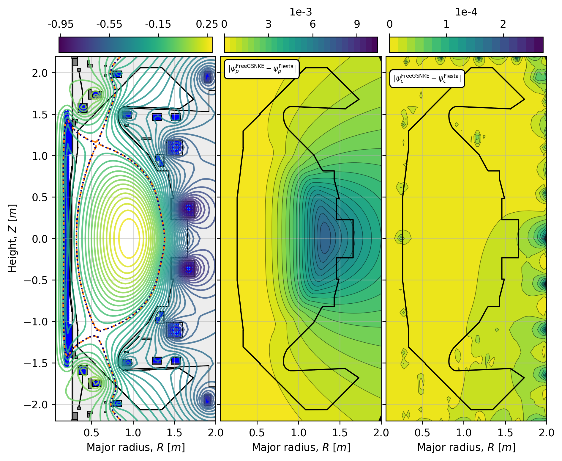
Figure 5.1: Simulated MAST-U shot 45425 ($t=0.7$s) equilibrium. Left: separatrices from both Fiesta (orange) and FreeGSNKE (dotted blue) equilibria alongside the FreeGSNKE $\psi$ contours. Centre: absolute difference in $\psi_{p}$ between the two codes. Right: same as centre but for $\psi_{c}$.

5.1 MAST-U shot 45425: Conventional divertor

We first simulate MAST-U shot 45425, which has a flat-top plasma current of approximately $750$kA, a double-null shape, and a conventional divertor configuration. The plasma is heated using two neutral beam injection systems delivering a total power of approximately $2.5$MW. The plasma is in H-mode confinement for the majority of the shot.

5.1.1 Single time slice

Before analysing the entire shot, we wish to briefly discuss and compare a few minor differences between the flux quantities produced by each code for a single time slice of the shot ($t=0.7$s). We begin by comparing FreeGSNKE and Fiesta without EFIT++ in Figure 5.1. The left panel displays the $\psi$ contours from FreeGSNKE and an almost perfect overlap of the separatrices from both codes.

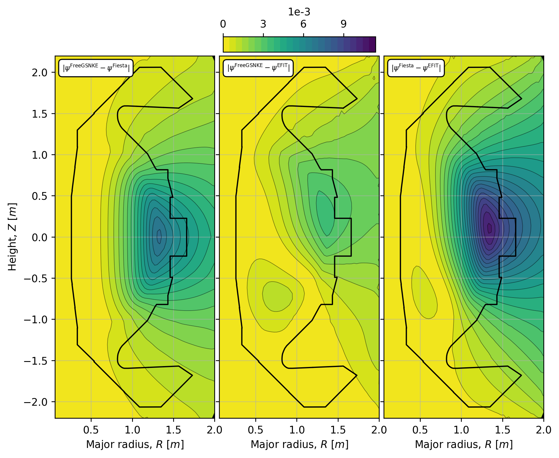
Figure 5.2: Differences in the total flux $\psi$ between all three codes for MAST-U shot 45425 ($t=0.7$s). Left: absolute difference in $\psi$ between FreeGSNKE and Fiesta. Centre: difference between FreeGSNKE and EFIT++. Right: difference between Fiesta and EFIT++.

We break this down in the centre and right panels. The right panel shows the magnitude of differences in $\psi_{c}$, the plasma flux generated by active coils and passive structures. It can be seen that differences are generally small, at a level of $\lesssim 2\text{e}\mathord{-}4$, compared to a total flux that spans a range $\max(\psi)-\min(\psi)\sim 1$. These differences appear co-localised with the vessel’s passive structures, suggesting they are driven by implementation details in the methods used by either code to distribute the passive structure currents over their poloidal sections. The central panel shows differences in the plasma flux $\psi_{p}$. The largest differences are localised in the top-right and bottom-right edge pixels of the discretised domain. We attribute this to implementation details in the way Fiesta imposes the boundary conditions (see also the right panel of Figure 5.2, where the same discrepancy is visible again). The remaining differences are at a level of $\lesssim 5\text{e}\mathord{-}3$. We believe these are largely due to implementation differences in the routines that identify the last closed flux surface of the plasma, rather than being due to the nonlinear solvers themselves. In fact, we find that a comparison between the plasma current density distributions $J_{p}$ calculated by FreeGSNKE and Fiesta for the same total flux $\psi$ results in differences of the same order of magnitude.

In Figure 5.2, we compare differences in the total flux $\psi$ between all three codes. The left panel is similar to the one seen in Figure 5.1 (centre), with differences between FreeGSNKE and Fiesta dominated by differences in $\psi_{p}$ as just discussed. Similarly to the differences between FreeGSNKE and Fiesta, the differences between FreeGSNKE/Fiesta and EFIT++ (shown in the centre/right panels, respectively) are largest close to the plasma outer edge, and qualitatively analogous (if not slightly different in magnitude).

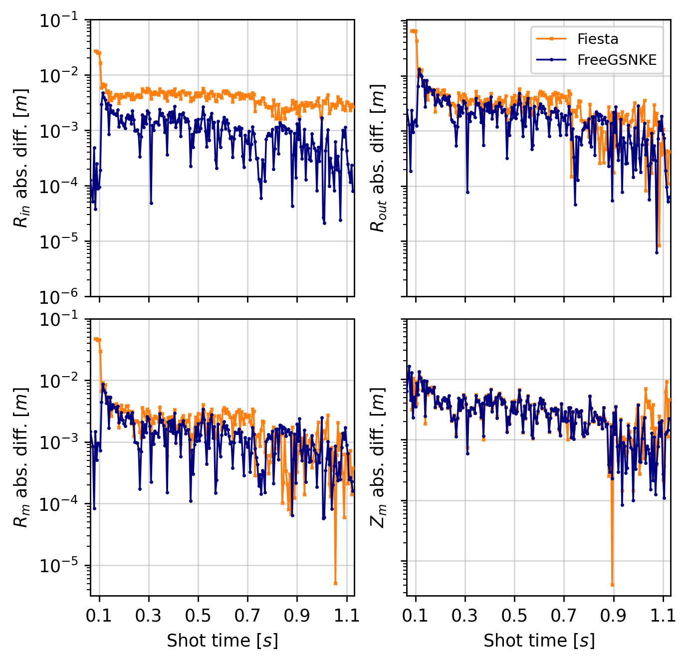
Figure 5.3: Absolute differences between EFIT++ and Fiesta (orange crosses)/FreeGSNKE (blue dots) shape targets. Top: absolute difference in midplane inner $R_{in}$ and outer $R_{out}$ radii. Bottom: absolute difference in magnetic axis components $R_{m}$ and $Z_{m}$.

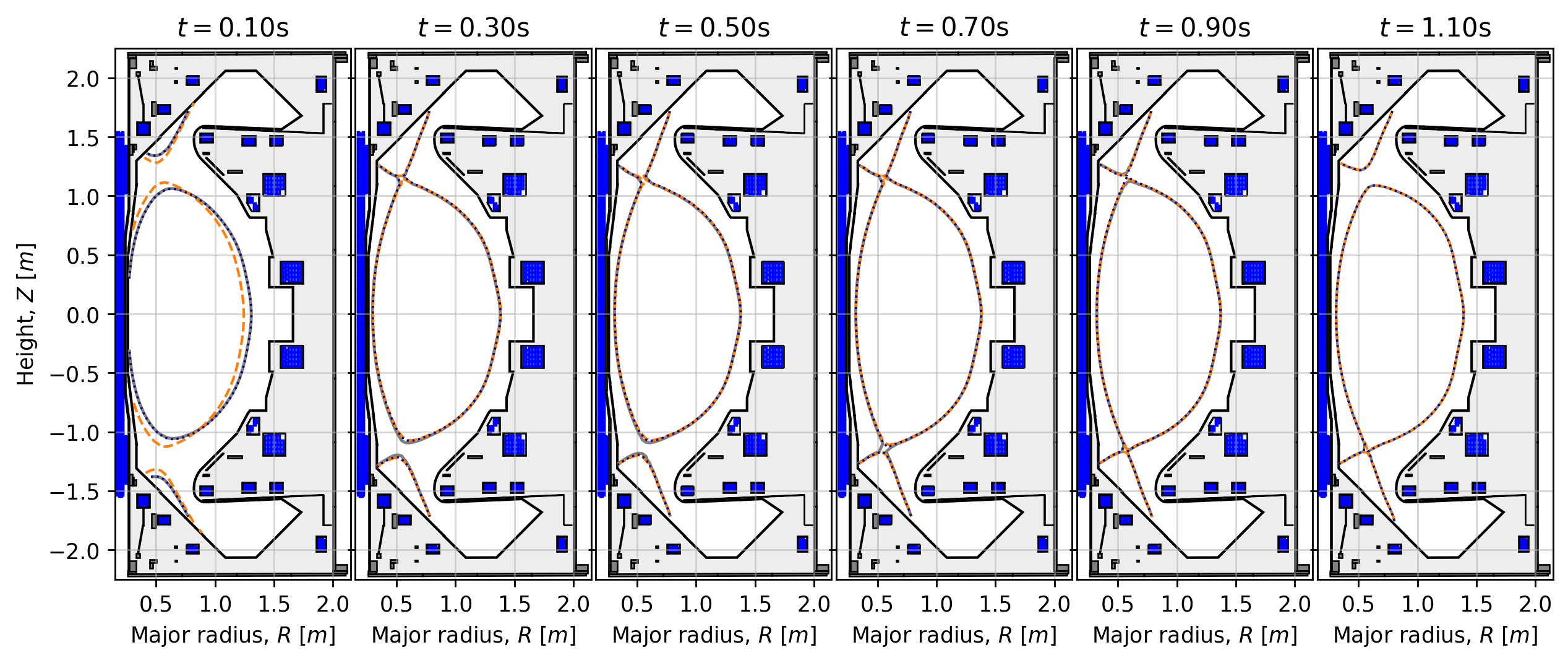
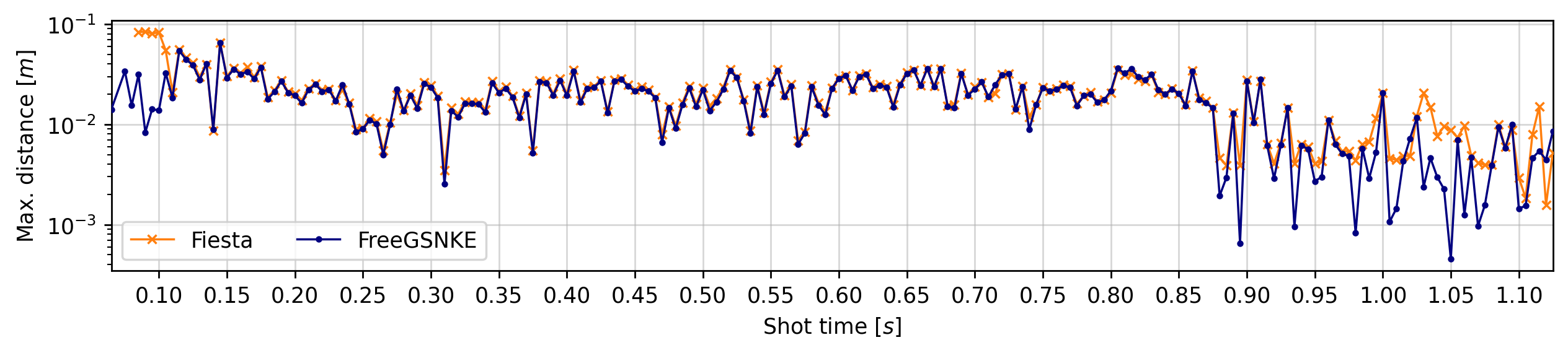
Figure 5.4: Top: evolution of EFIT++ (solid grey), Fiesta (dashed orange), and FreeGSNKE (dotted blue) separatrices at different shot times. Bottom: maximum Euclidean distance between any two corresponding $(R,Z)$ points on the EFIT++ and Fiesta/FreeGSNKE core separatrices (divertor legs not included).

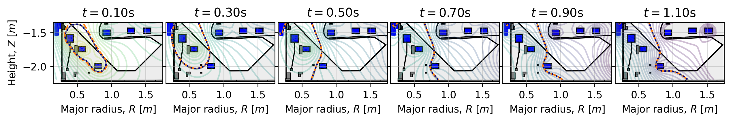
Figure 5.5: Top: evolution of EFIT++ (solid grey), Fiesta (dashed orange), and FreeGSNKE (dotted blue) lower divertor strikepoints at different shot times. Bottom: absolute difference between between EFIT++ and Fiesta/FreeGSNKE for $R_{s}$ (errors are at the same level for $Z_{s}$).

It is worth highlighting explicitly that the mismatches shown in Figure 5.1 and Figure 5.2 are, nominally, beyond the relative tolerance used in both FreeGSNKE and Fiesta—recall this was $\varepsilon=1\text{e}\mathord{-}6$. However, as already mentioned: i) differences in the implementation of the passive structures and ii) differences in routines that build the plasma core mask between the three codes at hand, are responsible for introducing mismatches with similar orders of magnitude to those we are seeing. Besides, as hinted by the left panel in Figure 5.1 and as we show in the following results, this level of difference has a negligible impact on the shape control targets (and therefore for most practical modelling purposes).

5.1.2 Entire shot

Over the course of the entire shot, the differences in $\psi$ (for both codes) remain at the levels seen in Figure 5.2. For FreeGSNKE, the median differences in $\psi_{a}$ and $\psi_{b}$ over the shot are $1\text{e}\mathord{-}3$ and $6\text{e}\mathord{-}4$, respectively. For Fiesta, the corresponding differences are on average $3\text{e}\mathord{-}3$ and $1\text{e}\mathord{-}3$, respectively.

In Figure 5.3, we plot the differences in the magnetic axis $(R_{m},Z_{m})$, the midplane inner radius $R_{in}$, and the midplane outer radius $R_{out}$ (recall Figure 4.1). Typical differences in the inner/outer radii are of the order of millimetres for FreeGSNKE, with only marginally higher values for Fiesta. With respect to the magnetic axis, differences in both codes vs. EFIT++ track one another to sub-centimetre precision as well. There are, however, some isolated times during the initial phase of the ramp up where the differences between Fiesta and EFIT++ are significantly higher (see similar differences in later plots) than in later time slices. While FreeGSNKE has found (precisely) the EFIT++ GS equilibria during these early slices, we suspect that Fiesta may have simply found another set of (equally valid) GS equilibria. The physical difference in these (limited, not yet diverted) equilibria can be seen more clearly in Figure 5.4 at $t=0.10s$. While we do not have a conclusive reason for the presence of multiple GS equilibria here (given the same input parameters), identifying under what conditions these equilibria co-exist may be worth further numerical investigation (ham2024).

In top panel of Figure 5.4, we plot the evolution of the separatrices produced by all three codes over the lifetime of the shot, observing an excellent match in the majority of shot times. The metric in the lower panel of Figure 5.4 is calculated by first finding $360$ $(R,Z)$ points on the core separatrix generated by each code, where each point is equally spaced in the geometric poloidal angle centred on the magnetic axis (of EFIT++). The largest distance between corresponding points on the FreeGSNKE/Fiesta separatrix and the EFIT++ separatrix is then measured. This maximum distance is below $3.5$cm in $95\%$ of cases for FreeGSNKE equilibria (in $96\%$ of cases the median distance is below $1$cm). For the case of Fiesta, the maximum distance is $4.2$cm for the same quantile ($1.13$cm for the median distance for the same quantile of $96\%$ of cases). Any gaps in the time series (and in later plots) are where Fiesta failed to converge to an equilibrium given the tolerance $\varepsilon$—these time slices have been excluded when calculating the quantiles mentioned above. We would note that during these times slices (where the equilibrium is in a limiter-type configuration), Fiesta can converge when using the feedback2 object mentioned in Section 4.

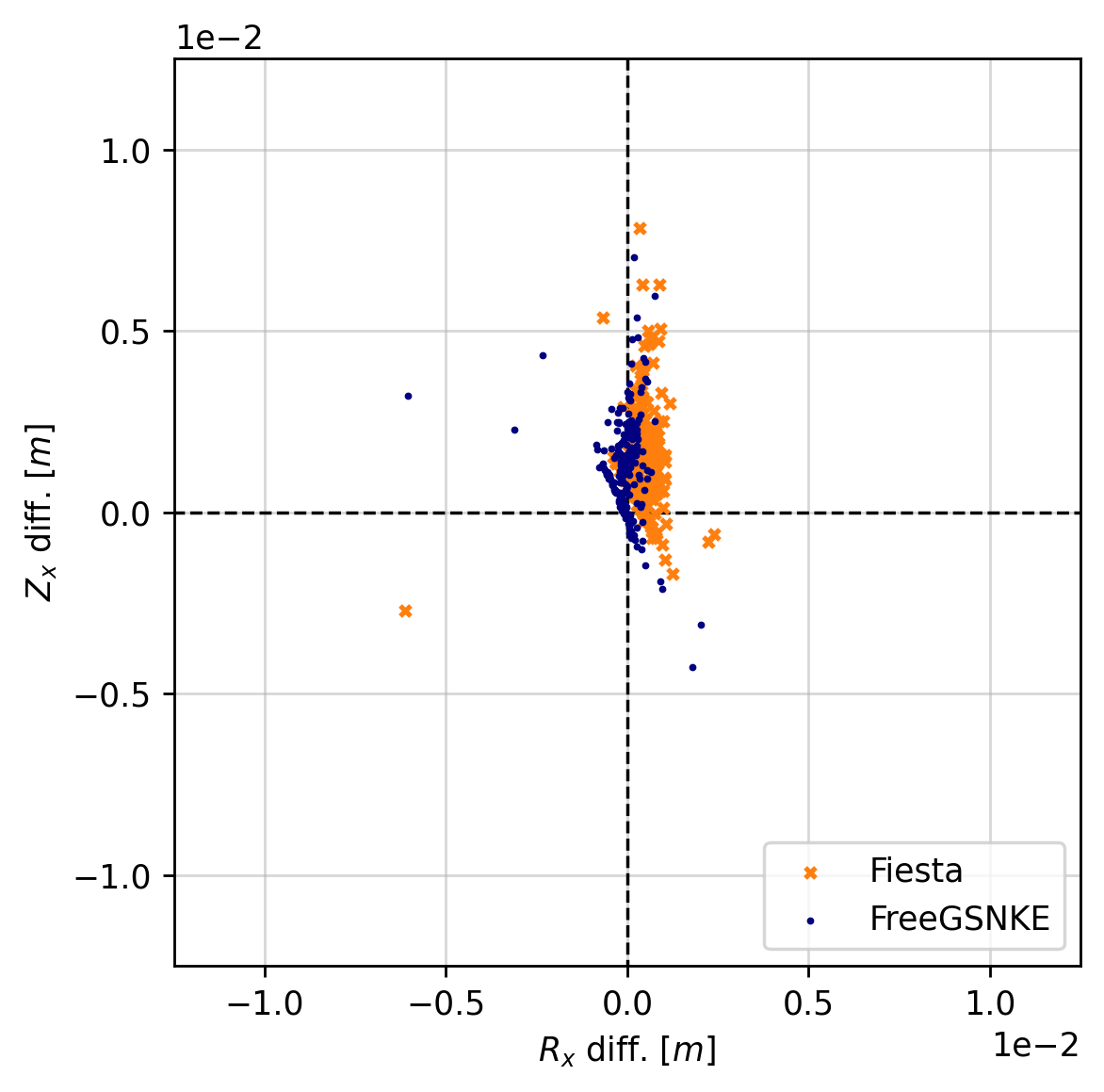
Figure 5.6: Difference between EFIT++ and Fiesta (orange crosses)/FreeGSNKE (blue dots) lower core chamber X-points (over the entire shot).

In Figure 5.5 we monitor the evolution of a strikepoint along the lower divertor tiles, again, observing an excellent match from both codes. The difference in $(R_{s},Z_{s})$ compared to EFIT++ is less than a centimetre for most of the shot—very early times being the exception in the case of Fiesta. Note that while the difference in $Z_{s}$ is not explicitly shown, it looks almost exactly the same as that of $R_{s}$.

In Figure 5.6, we plot the difference in the lower core chamber X-point over the shot. As we did for the separatrix calculations, we identify all X-points for each code’s equilibria using FreeGSNKE’s build-in functionality. This was because Fiesta and EFIT++ would inconsistently return only a single X-point, sometimes in the lower core chamber, sometime the upper. There appears to be a small vertical bias towards higher X-points by a few millimetres in both Fiesta and FreeGSNKE—also visible in some of the upper panels of Figure 5.4. Despite this slight bias, both codes are accurate with respect to EFIT++ to within half a centimetre for $98\%$ and $97\%$ of the shot, respectively ($100\%$ are within $1$cm).

The runtimes, both per time slice and cumulatively across the shot, are displayed in Figure 5.7. Median runtimes are $6.7\text{\,}\mathrm{s}$ per forward solve for Fiesta, $0.09\text{\,}\mathrm{s}$ for FreeGSNKE. Fiesta is significantly hindered by the use of the feedback3 object which demands a second nonlinear solver loop to stabilise the Picard iterations. FreeGSNKE makes use of the faster and more stable convergence of the Newton–Krylov method, as well as using numba just-in-time compilation for some core routines. As mentioned before, all equilibria were simulated sequentially with both codes. However, given the independence of each time slice, nothing prevents an embarrassingly parallel implementation—though this was not an objective in this paper.

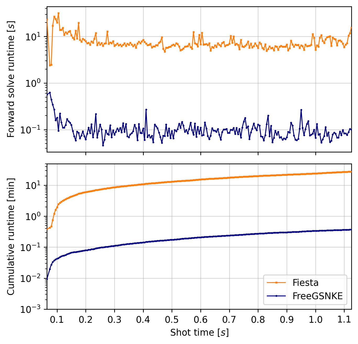
Figure 5.7: Fiesta (orange) and FreeGSNKE (blue) forward solve runtimes over the shot (in seconds). Top: runtime per forward solve. Bottom: cumulative runtime of forward solves (in total, Fiesta takes $27\text{\,}\mathrm{min}$ $48\text{\,}\mathrm{s}$ and FreeGSNKE takes $22\text{\,}\mathrm{s}$.

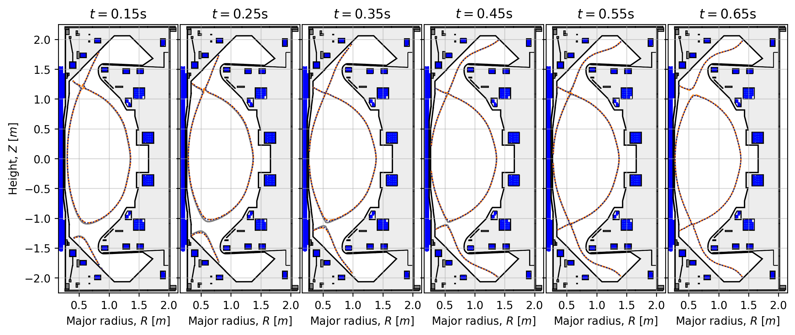
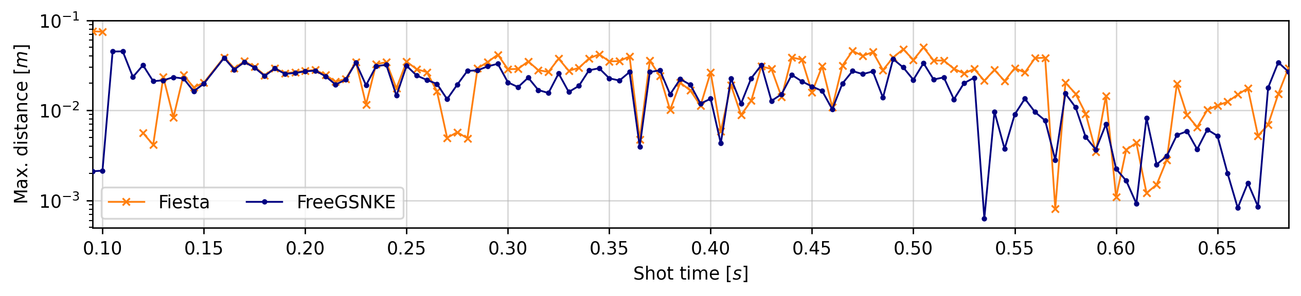
Figure 5.8: Top: evolution of EFIT++ (solid grey), Fiesta (dashed orange), and FreeGSNKE (dotted blue) separatrices at different shot times. Bottom: maximum Euclidean distance between any two corresponding $(R,Z)$ points on the EFIT++ and Fiesta/FreeGSNKE core separatrices (divertor legs not included).

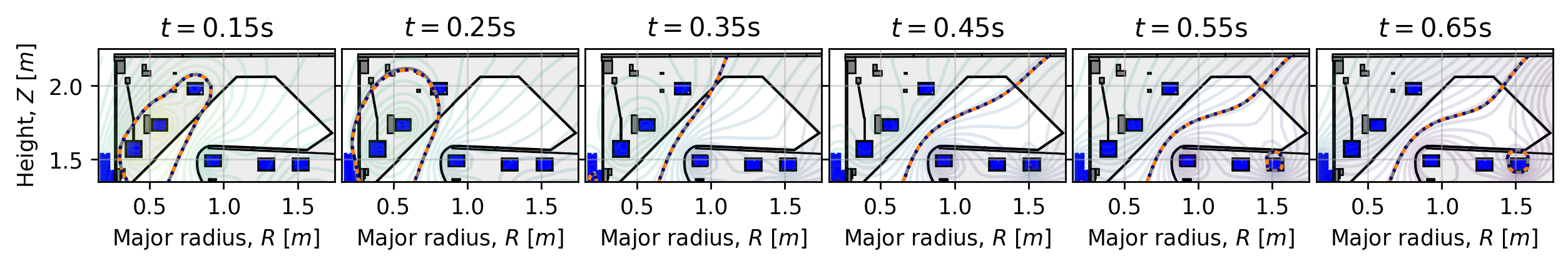
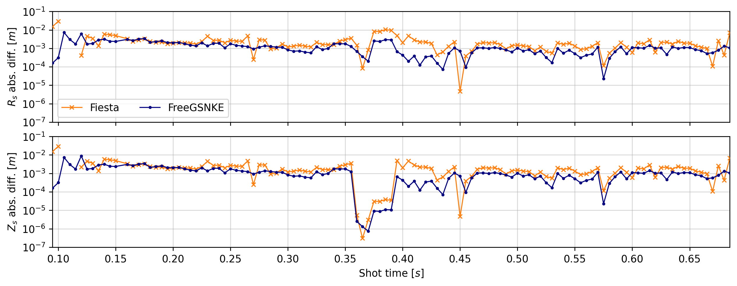
Figure 5.9: Top: evolution of EFIT++ (solid grey), Fiesta (dashed orange), and FreeGSNKE (dotted blue) lower divertor strikepoints at different shot times. Centre: absolute difference between between EFIT++ and Fiesta/FreeGSNKE for $R_{s}$. Bottom: same as centre but for $Z_{s}$.

5.2 MAST-U shot 45292: Super-X divertor

Here, we focus on MAST-U shot $45292$, which has a flat-top plasma current of approximately $750$kA, a double-null shape, and a Super-X divertor configuration. The plasma is Ohmically heated, i.e. there is no neutral beam heating, and remains in the L-mode confinement regime throughout the shot.

As we did for the previous shot, we plot the evolution of the separatrices from all three codes over time in Figure 5.8, again discerning a very good agreement between all of them (including qualitatively on the divertor legs). Given the Super-X configuration, the upper divertor strikepoint now evolves across the tiles. We can see, in Figure 5.9, good agreement with differences in $R_{s}$ and $Z_{s}$ remaining at similar levels (though marginally different).

Differences in the poloidal flux quantities remain at the same levels as seen in the conventional divertor shot while the shape targets again match to sub-centimetre precision—see Figure 5.10. The upper core chamber X-points from FreeGSNKE and Fiesta are again accurate to within half a centimetre for $92\%$ and $87\%$ of time slices shown ($100\%$ within $1$cm), respectively (see Figure 5.11). Runtimes for both simulations were almost identical to those seen in the previous experiment and are therefore not shown again. To see the additional results not shown here for the Super-X shot, refer to the code repository.

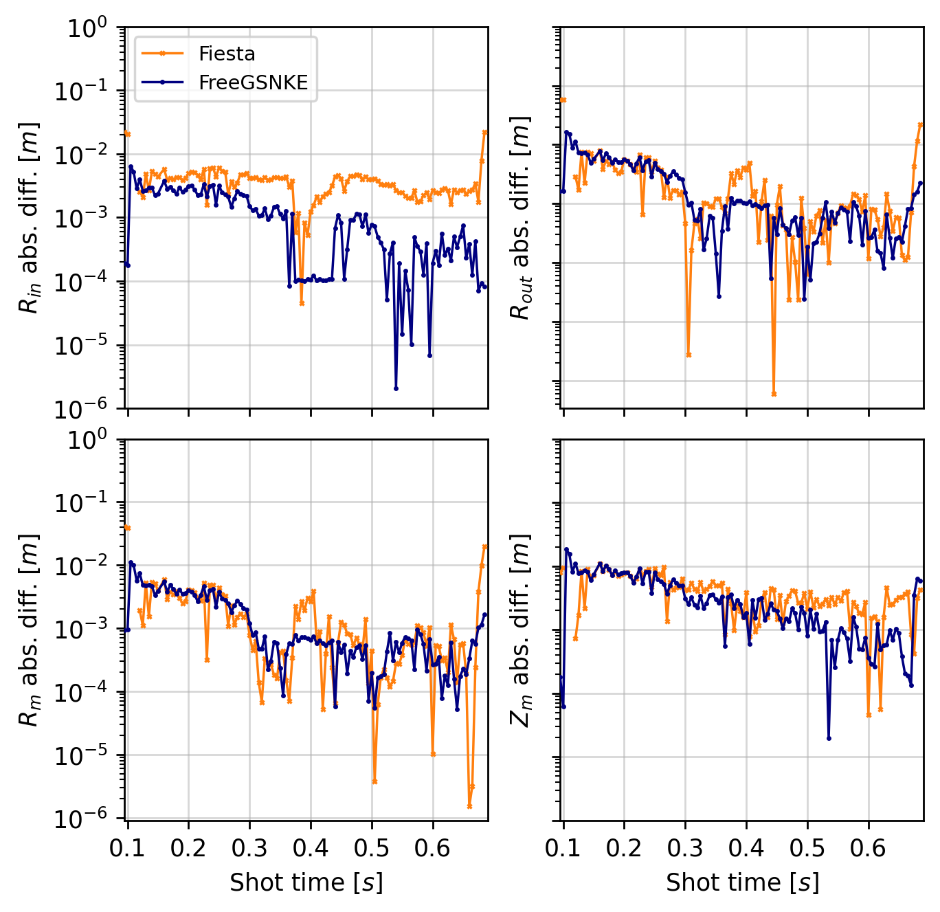
Figure 5.10: Absolute differences between EFIT++ and Fiesta (orange crosses)/FreeGSNKE (blue dots) shape targets. Top: absolute difference in midplane inner $R_{in}$ and outer $R_{out}$ radii. Bottom: absolute difference in magnetic axis components $R_{m}$ and $Z_{m}$.

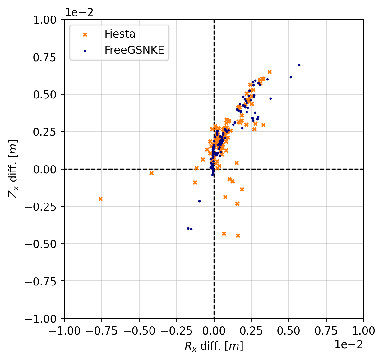
Figure 5.11: Absolute differences between EFIT++ and Fiesta (orange crosses)/FreeGSNKE (blue dots) lower core chamber X-points (over entire shot).

6 Conclusions

In this paper, we have demonstrated that the static forward GS solvers (see Section 3) in FreeGSNKE and Fiesta can accurately reproduce equilibria generated by magnetics-only EFIT++ reconstructions on MAST-U.

To achieve this, we began (Section 4) by outlining which features of the MAST-U machine would be included in the forward solver machine descriptions, using those that most closely matched the one by EFIT++. We highlighted the capability of both codes being able to model the active poloidal field coils as either up/down symmetric or asymmetric, noting that EFIT++ uses the asymmetric setting. In addition, both codes have the option to refine passive structures into smaller filaments in order to distribute the induced current in them across their surface areas for better electromagnetic modelling. Following this, we set the conductor currents and prescribed appropriate plasma current density profiles—in this case the polynomial-based “Lao” profiles whose coefficients are determined by EFIT++. In addition to some other code-specific parameters, we then used this computational pipeline to begin simulating the MAST-U equilibria.

The poloidal flux quantities and shape targets generated by the FreeGSNKE and Fiesta simulations in Section 5 show excellent agreement with the corresponding quantities from EFIT++ for both MAST-U shots tested. More specifically, separatrices from both codes match those of EFIT++, with the largest distances between the core separatrices found to be on the order of centimetres. Strikepoints, X-points, magnetic axes, and inner/outer midplane radii differences between the codes were simulated to sub-centimetre precision.

The static GS solver in FreeGSNKE has now been validated against both analytic equilibria (see Amorisco et al. (2024)) and experimental reconstructions from MAST-U (this paper). It has also been shown to produce numerically equivalent equilbria to the Fiesta code, which itself has been validated on experimentally reconstructed equilibria from a number of different tokamak devices (refer back to Section 1). Given its user-friendly Python interface, we hope that this work will enable the more widespread adoption of FreeGSNKE for real-time plasma control and optimisation studies (including those with a machine learning element) and assist in the design of future fusion power plants. Furthermore, we hope that the code and datasets made available with this paper will be of use in validation studies for other equilibrium modelling codes. Some avenues for future work include validating the dynamic forward GS solver in FreeGSNKE using real-world plasma reconstructions, incorporating more complex/unconstrained plasma profile functions, and making use of data assimilation techniques to carry out probabilistic (uncertainty-aware) equilibrium reconstruction.

Data availability

The code scripts and data used in this paper will be made available in due course.

Declarations

The authors have no conflicts of interest to declare.

References

- Agnello et al. (2024) A. Agnello, N. C. Amorisco, A. Keats, G. K. Holt, J. Buchanan, S. Pamela, C. Vincent, and G. McArdle. Emulation techniques for scenario and classical control design of tokamak plasmas. Physics of Plasmas, 31(4):043901, 2024. 10.1063/5.0187822.
- Amorisco et al. (2024) N. C. Amorisco, A. Agnello, G. Holt, M. Mars, J. Buchanan, and S. Pamela. FreeGSNKE: A python-based dynamic free-boundary toroidal plasma equilibrium solver. Physics of Plasmas, 31(4):042517, 2024. 10.1063/5.0188467.
- Appel and Lupelli (2018) L. C. Appel and I. Lupelli. Equilibrium reconstruction in an iron core tokamak using a deterministic magnetisation model. Computer Physics Communications, 223:1–17, 2018. 10.1016/j.cpc.2017.09.016.
- Appel et al. (2001) L. C. Appel, M. K. Bevir, and M. J. Walsh. Equilibrium reconstruction in the START tokamak. Nuclear Fusion, 41(2):169, 2001. 10.1088/0029-5515/41/2/303.
- Appel et al. (2006) L. C. Appel, G. T. A. Huysmans, L. L. Lao, P. J. McCarthy, D. G. Muir, E. R. Solano, J. Storrs, D. Taylor, and W. Zwingmann. A unified approach to equilibrium reconstruction. In Proceedings of the 33rd EPS Conference, 2006.
- Araya-Solano et al. (2021) L. Araya-Solano, V. I. Vargas, R. Solano-Piedra, A. A. Ramírez, M. Hernández-Cisneros, F. Coto-Vílchez, M. A. Rojas-Quesada, J. E. Pérez-Hidalgo, and F. Vílchez-Coto. Implementation of the spherical tokamak MEDUSA-CR. In Proceedings of the 8th International Conference, pages EX/P7–22, 2021.
- Artaud and Kim (2012) J. F. Artaud and S. H. Kim. A new free-boundary equilibrium evolution code, FREEBIE. In 39th EPS Conference & 16th Int. Congress on Plasma Physics, pages 1178–1181, 2012.
- Bao et al. (2023) N. Bao, X. Yan, S. Wei, and Z. Wang. Py-EFIT: a new python package for plasma equilibrium reconstruction on EAST tokamak. Computer Physics Communications, 282:108549, 2023. 10.1016/j.cpc.2022.108549.
- Berkery et al. (2021) J. W. Berkery, S. A. Sabbagh, L. Kogan, D. Ryan, J. M. Bialek, Y. Jiang, D. J. Battaglia, S. Gibson, and C. Ham. Kinetic equilibrium reconstructions of plasmas in the MAST database and preparation for reconstruction of the first plasmas in MAST upgrade. Plasma Physics and Controlled Fusion, 63(5):055014, 2021. 10.1088/1361-6587/abf230.
- Carpanese (2021) F. Carpanese. Development of free-boundary equilibrium and transport solvers for simulation and real-time interpretation of tokamak experiments. PhD thesis, EPFL, 2021.
- Cerfon and Freidberg (2010) A. J. Cerfon and J. P. Freidberg. “One size fits all” analytic solutions to the Grad–Shafranov equation. Physics of Plasmas, 17(3):032502, 2010. 10.1063/1.3328818.
- Coleman and McIntosh (2020) M. Coleman and S. McIntosh. The design and optimisation of tokamak poloidal field systems in the BLUEPRINT framework. Fusion Engineering and Design, 154:111544, 2020. 10.1016/j.fusengdes.2020.111544.
- Coutlis et al. (1999) A. Coutlis, I. Bandyopadhyay, J. B. Lister, P. Vyas, R. Albanese, D. J. N. Limebeer, F. Villone, and J. P. Wainwright. Measurement of the open loop plasma equilibrium response in TCV. Nuclear Fusion, 39(5), 1999. 10.1088/0029-5515/39/5/307.
- Creely et al. (2020) A. J. Creely, M. J. Greenwald, S. B. Ballinger, D. Brunner, J. Canik, J. Doody, T. Fülöp, D. T. Garnier, R. Granetz, T. K. Gray, C. Holland, N. T. Howard, J. W. Hughes, J. H. Irby, V. A. Izzo, G. J. Kramer, A. Q. Kuang, B. LaBombard, Y. Lin, B. Lipschultz, N. C. Logan, J. D. Lore, E. S. Marmar, K. Montes, R. T. Mumgaard, C. Paz-Soldan, C. Rea, M. L. Reinke, P. Rodriguez-Fernandez, K. Särkimäki, F. Sciortino, S. D. Scott, A. Snicker, P. B. Snyder, B. N. Sorbom, R. Sweeney, R. A. Tinguely, E. A. Tolman, M. Umansky, O. Vallhagen, J. Varje, D. G. Whyte, J. C. Wright, S. J. Wukitch, J. Zhu, and t. Team. Overview of the SPARC tokamak. Journal of Plasma Physics, 86(5):865860502, 2020. 10.1017/S0022377820001257.
- Cunningham (2013) G. Cunningham. High performance plasma vertical position control system for upgraded MAST. Fusion Engineering and Design, 88(12):3238–3247, 2013. 10.1016/j.fusengdes.2013.10.001.
- de Boucaud et al. (2022) N. de Boucaud, T. Golfinopoulos, and A. Marinoni. On the synergy between easier plasma operation and affordable coil-set requirements enabled by negative triangularity in the prospective ARC fusion reactor, 2022. arXiv:2212.08218.
- Doyle et al. (2021) S. J. Doyle, D. Lopez-Aires, A. Mancini, M. Agredano-Torres, J. L. Garcia-Sanchez, J. Segado-Fernandez, J. Ayllon-Guerola, M. Garcia-Muñoz, E. Viezzer, C. Soria-Hoyo, J. Garcia-Lopez, G. Cunningham, P. F. Buxton, M. P. Gryaznevich, Y. S. Hwang, and K. J. Chung. Magnetic equilibrium design for the SMART tokamak. Fusion Engineering and Design, 171:112706, 2021. 10.1016/j.fusengdes.2021.112706.
- Dudson (2024) B. Dudson. FreeGS: Free-boundary Grad-Shafranov solver, 2024. URL https://github.com/freegs-plasma/freegs.
- Grad and Rubin (1958) H. Grad and H. Rubin. Hydromagnetic equilibria and force-free fields. In Proceedings of the Second United Nations International Conference on the Peaceful Uses of Atomic Energy: Theoretical and experimental aspects of controlled nuclear fusion, volume 31, page 400. United Nations, 1958.
- Hudoba et al. (2023) A. Hudoba, G. Cunningham, and S. Bakes. Magnetic equilibrium optimisation and divertor integration in spherical tokamak reactors. Fusion Engineering and Design, 191:113704, 2023. 10.1016/j.fusengdes.2023.113704.
- Jardin (2010) S. Jardin. Computational Methods in Plasma Physics. CRC Press, 2010. 10.1201/EBK1439810958.
- Jeon (2015) Y. M. Jeon. Development of a free-boundary tokamak equilibrium solver for advanced study of tokamak equilibria. Journal of the Korean Physical Society, 67(5):843–853, 2015. 10.3938/jkps.67.843.
- Kelley (1995) C. T. Kelley. Iterative Methods for Linear and Nonlinear Equations. SIAM, 1995.
- Knoll and Keyes (2004) D. A. Knoll and D. E. Keyes. Jacobian-free Newton-Krylov methods: a survey of approaches and applications. Journal of Computational Physics, 193(2):357–397, 2004. 10.1016/j.jcp.2003.08.010.
- Kogan et al. (2021) L. Kogan, D. Ryan, J. Berkery, S. Sabbagh, J. M. Blalek, L. Appel, R. Scannell, T. Farley, A. Thornton, and G. Cunningham. EFIT++ reconstructions for MAST-U. MUDDMC, 2021.
- Kripner et al. (2018) L. Kripner, M. Peterka, M. Imríšek, T. Markovič, J. Urban, J. Havlíček, M. Hron, F. Jaulmes, R. Pánek, D. Šestík, V. Weinzettl, V. Yanovskiy, and the COMPASS Team. Equilibrium design for the COMPASS-U tokamak. In WDS’18 Proceedings of Contributed Papers — Physics, pages 99–104, 2018.
- Lao et al. (1985) L. L. Lao, H. S. John, R. D. Stambaugh, A. G. Kellman, and W. Pfeiffer. Reconstruction of current profile parameters and plasma shapes in tokamaks. Nuclear Fusion, 25(11):1611, 1985. 10.1088/0029-5515/25/11/007.
- Lao et al. (2005) L. L. Lao, H. E. S. John, Q. Peng, J. R. Ferron, E. J. Strait, T. S. Taylor, W. H. Meyer, C. Zhang, and K. I. You. MHD equilibrium reconstruction in the DIII-D tokamak. Fusion Science and Technology, 48(2):968–977, 2005. 10.13182/FST48-968.
- Lao et al. (2022) L. L. Lao, S. Kruger, C. Akcay, P. Balaprakash, T. A. Bechtel, E. Howell, J. Koo, J. Leddy, M. Leinhauser, Y. Q. Liu, S. Madireddy, J. McClenaghan, D. Orozco, A. Pankin, D. Schissel, S. Smith, X. Sun, and S. Williams. Application of machine learning and artificial intelligence to extend EFIT equilibrium reconstruction. Plasma Physics and Controlled Fusion, 64(7):074001, 2022. 10.1088/1361-6587/ac6fff.
- Lee et al. (1999) B. Lee, N. Pomphrey, and L. L. Lao. Physics design of poloidal field, toroidal field, and external magnetic diagnostics in KSTAR. Fusion Technology, 36(3):278–288, 1999. 10.13182/FST99-A108.
- Lee et al. (2021) C. Y. Lee, J. Seo, S. J. Park, J. G. Lee, S. K. Kim, B. Kim, C. S. Byun, Y. S. Lee, J. W. Gwak, J. Kang, L. Jung, H. S. Kim, S. H. Hong, and Y.-S. Na. Development of integrated suite of codes and its validation on KSTAR. Nuclear Fusion, 61(9):096020, 2021. 10.1088/1741-4326/ac1690.
- Mancini et al. (2023) A. Mancini, L. Velarde, E. Viezzer, D. J. Cruz-Zabala, J. F. Rivero-Rodriguez, M. Garcia-Muñoz, L. Sanchis, A. Snicker, J. Segado-Fernandez, J. Garcia-Dominguez, J. Hidalgo-Salaverri, P. Cano-Megias, and M. Toscano-Jimenez. Predictive simulations for plasma scenarios in the SMART tokamak. Fusion Engineering and Design, 192:113833, 2023. 10.1016/j.fusengdes.2023.113833.
- MANTA Team (2023) MANTA Team. Modular adjustable negative-triangularity ARC (MANTA): A fusion pilot plant. USBPO Webinar, 2023.
- Maquet et al. (2023) V. Maquet, R. Ragona, D. van Eester, J. Hillairet, and F. Durodie. ANSYS HFSS as a new numerical tool to study wave propagation inside anisotropic magnetized plasmas in the ion cylotron range of frequencies, 2023. arXiv:309.14015.
- MAST Upgrade Team et al. (2022) MAST Upgrade Team, L. Kogan, S. Gibson, D. Ryan, C. Bowman, A. Kirk, J. Berkery, S. Sabbagh, T. Farley, P. Ryan, C. Wade, K. Verhaegh, B. Kool, T. Wijkamp, R. Scannell, and R. Sarwar. First MAST-U equilibrium reconstructions using the EFIT++ code. In 48th European Physical Society Conference on Plasma Physics, 2022.
- McArdle and Taylor (2008) G. J. McArdle and D. Taylor. Adaptation of the MAST passive current simulation model for real-time plasma control. Fusion Engineering and Design, 83(2):188–192, 2008. 10.1016/j.fusengdes.2007.11.003.
- Morris et al. (2021) J. Morris, S. Muldrew, M. Kovari, S. Kahn, and A. Pearce. Preparing the systems code process for EU-DEMO conceptual design. In 28th IAEA Fusion Energy Conference, Nice, France (Virtual), pages 10–15, 2021.
- Morris et al. (2014) W. Morris, J. Milnes, T. Barrett, C. Challis, I. Chapman, M. Cox, G. Cunningham, F. Dhalla, G. Fishpool, P. Jacquet, I. Katramados, A. Kirk, K. McClements, R. Martin, H. Meyer, M. Romanelli, S. Saarelma, S. Sharapov, V. Thompson, M. Valovič, G. Whitfield, and D. Wolff. MAST accomplishments and upgrade for fusion next-steps. IEEE Transactions on Plasma Science, 42(3):402–414, 2014. 10.1109/TPS.2014.2299973.
- Morris et al. (2018) W. Morris, J. R. Harrison, A. Kirk, B. Lipschultz, F. Militello, D. Moulton, and N. R. Walkden. MAST upgrade divertor facility: a test bed for novel divertor solutions. IEEE Transactions on Plasma Science, 46(5):1217–1226, 2018. 10.1109/TPS.2018.2815283.
- Ryan et al. (2023) D. A. Ryan, R. Martin, L. Appel, N. B. Ayed, L. Kogan, A. Kirk, and MAST Upgrade Team. Initial progress of the magnetic diagnostics of the MAST-U tokamak. The Review of Scientific Instruments, 94(7):073501, 2023. 10.1063/5.0156334.
- Sabbagh et al. (2001) S. A. Sabbagh, S. M. Kaye, J. Menard, F. Paoletti, M. Bell, R. E. Bell, J. M. Bialek, M. Bitter, E. D. Fredrickson, D. A. Gates, A. H. Glasser, H. Kugel, L. L. Lao, B. P. LeBlanc, R. Maingi, R. J. Maqueda, E. Mazzucato, D. Mueller, M. Ono, S. F. Paul, M. Peng, C. H. Skinner, D. Stutman, G. A. Wurden, W. Zhu, and t. Team. Equilibrium properties of spherical torus plasmas in NSTX. Nuclear Fusion, 41(11):1601, 2001. 10.1088/0029-5515/41/11/309.
- Sangaroon et al. (2023) S. Sangaroon, K. Ogawa, M. Isobe, A. Wisitsorasak, W. Paenthong, J. Promping, N. Poolyarat, A. Tamman, K. Ploykrachang, S. Dangtip, and T. Onjun. Feasibility study of neutral beam injection in Thailand Tokamak-1. Fusion Engineering and Design, 188:113419, 2023. 10.1016/j.fusengdes.2023.113419.
- Shafranov (1958) V. D. Shafranov. On magnetohydrodynamical equilibrium configurations. Soviet Journal of Experimental and Theoretical Physics, 6:545, 1958.
- Vondracek et al. (2021) P. Vondracek, R. Panek, M. Hron, J. Havlicek, V. Weinzettl, T. Todd, D. Tskhakaya, G. Cunningham, P. Hacek, J. Hromadka, P. Junek, J. Krbec, N. Patel, D. Sestak, J. Varju, J. Adamek, M. Balazsova, V. Balner, P. Barton, J. Bielecki, P. Bilkova, J. Błocki, D. Bocian, K. Bogar, O. Bogar, P. Boocz, I. Borodkina, A. Brooks, P. Bohm, J. Burant, A. Casolari, J. Cavalier, P. Chappuis, R. Dejarnac, M. Dimitrova, M. Dudak, I. Duran, R. Ellis, S. Entler, J. Fang, M. Farnik, O. Ficker, D. Fridrich, S. Fukova, J. Gerardin, I. Hanak, A. Havranek, A. Herrmann, J. Horacek, O. Hronova, M. Imrisek, N. Isernia, F. Jaulmes, M. Jerab, V. Kindl, M. Komm, K. Kovarik, M. Kral, L. Kripner, E. Macusova, T. Majer, T. Markovic, E. Matveeva, K. Mikszuta-Michalik, M. Mohelnik, I. Mysiura, D. Naydenkova, I. Nemec, R. Ortwein, K. Patocka, M. Peterka, A. Podolnik, F. Prochazka, J. Prevratil, J. Reboun, V. Scalera, M. Scholz, J. Svoboda, J. Swierblewski, M. Sos, M. Tadros, P. Titus, M. Tomes, A. Torres, G. Tracz, P. Turjanica, M. Varavin, V. Veselovsky, F. Villone, P. Wachal, V. Yanovskiy, G. Zadvitskiy, J. Zajac, A. Zak, D. Zaloga, J. Zelda, and H. Zhang. Preliminary design of the COMPASS upgrade tokamak. Fusion Engineering and Design, 169:112490, 2021. 10.1016/j.fusengdes.2021.112490.
- Windridge et al. (2011) M. J. Windridge, G. Cunningham, T. C. Hender, R. Khayrutdinov, and V. Lukash. Non-linear instability at large vertical displacements in the MAST tokamak. Plasma Physics and Controlled Fusion, 53(3):035018, 2011. 10.1088/0741-3335/53/3/035018.
- Yoshida et al. (1986) H. Yoshida, H. Ninomiya, M. Azumi, and S. Seki. Numerical method for tokamak equilibrium with outside limiter. Journal of Computational Physics, 63(2):477–485, 1986. 10.1016/0021-9991(86)90205-6.