Not All Frequencies Are Created Equal:
Towards a Dynamic Fusion of Frequencies in Time-Series Forecasting

Abstract.

Long-term time series forecasting is a long-standing challenge in various applications. A central issue in time series forecasting is that methods should expressively capture long-term dependency. Furthermore, time series forecasting methods should be flexible when applied to different scenarios. Although Fourier analysis offers an alternative to effectively capture reusable and periodic patterns to achieve long-term forecasting in different scenarios, existing methods often assume high-frequency components represent noise and should be discarded in time series forecasting. However, we conduct a series of motivation experiments and discover that the role of certain frequencies varies depending on the scenarios. In some scenarios, removing high-frequency components from the original time series can improve the forecasting performance, while in others scenarios, removing them is harmful to forecasting performance. Therefore, it is necessary to treat the frequencies differently according to specific scenarios. To achieve this, we first reformulate the time series forecasting problem as learning a transfer function of each frequency in the Fourier domain. Further, we design Frequency Dynamic Fusion (FreDF), which individually predicts each Fourier component, and dynamically fuses the output of different frequencies. Moreover, we provide a novel insight into the generalization ability of time series forecasting and propose the generalization bound of time series forecasting. Then we prove FreDF has a lower bound, indicating that FreDF has better generalization ability. Extensive experiments conducted on multiple benchmark datasets and ablation studies demonstrate the effectiveness of FreDF.

1. Introduction

Time series forecasting is a well-established problem in various fields including energy usage (Bilal et al., 2022), economic planning (Ariyo et al., 2014), weather alerts (Duchon and Hale, 2012), and traffic forecasting (Li et al., 2015). With the development of deep learning (LeCun et al., 2015), numerous methods have emerged for this forecasting tasks (Zhu et al., 2023; Hu and Xiao, 2022; Bai et al., 2018; Wen et al., 2023; Guo et al., 2023). A central issue in time series forecasting is that existing methods could not expressively capture long-term dependency, which is often characterized as periodicity and trends (Li et al., 2021c; Box et al., 2015; Winters, 1960; Hamilton, 2020; Cheng et al., 2023). However, Fourier analysis has the strong potential to deal with long-term dependency, thereby makes related methods more flexible when adapted to different sequence prediction scenarios (Woo et al., 2022).

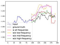
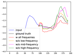
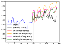
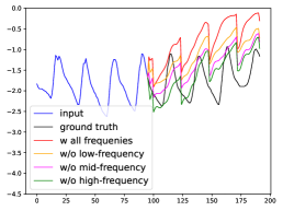
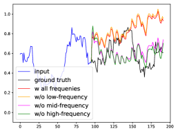
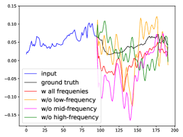
Figure 1. The comparison of prediction results using different frequencies on different datasets. (a) ETTm1; (b)ETTm2; (c)ETTh1; (d)ETTh2; (e) Exchange-rate; (f) Weather.

In the realm of TFS, an effective approach to addressing long-term dependency is to utilize Fourier analysis (Zhou et al., 2022b; Woo et al., 2022; Zhou et al., 2022a; Wu et al., 2023; Liu et al., 2023b). Fourier analysis is a powerful method that represents complex time series as a series of cosine functions, each with its unique frequency (Bracewell, 1986). This capability to represent infinitely long-term trends with a finite set of frequency components makes it efficient when applied to long-term time series forecasting.

Existing methods based on Fourier analysis often assume that high-frequency components represent noise and should be discarded during forecasting tasks (Zhou et al., 2022a; Xu et al., 2024). Additionally, some methods treat all frequencies equally, without considering their varying importance across different scenarios (Yi et al., 2023c, b). However, we argue that the role of certain frequencies varies in different scenarios. To validate this assumption, we conduct experiments on three datasets, eliminating low, middle, and high-frequency components respectively from the input of the training set to train a vanilla Transformer (Vaswani et al., 2017). The results, depicted in Figure 1, suggest that eliminating certain frequencies may improve performance in specific datasets while decreasing in others. In Exchange-rate(Figure 1(e)), we get more accurate prediction results after eliminating high frequencies. But it is less precise in Figure 1(b). The same phenomenon occurs at other frequencies. More detailed experimental setup and analysis are provided in Section 3.

These findings emphasize that simply marking high-frequency components as noise is undesirable. Without prior knowledge, determining which frequencies compose noise remains uncertain (Hamilton, 2020). Consequently, it is necessary to utilize different frequencies for forecasting and assign more rational weights to these forecasting results to improve the final prediction.

To separately assess the impact of different frequencies, it is necessary to predict each frequency individually. To begin with, we propose a mathematical reformulation of the TFS task in the Fourier domain. Then we propose Frequency Dynamic Fusion (FreDF), a novel framework to process time series datasets in decomposition, forecasting, and dynamic fusion, which individually forecasts each Fourier component, and dynamically fuses the output of different frequencies. The advantage of dynamic fusion lies in its capacity to flexibly adjust the weights of each frequency component, leading to more precise predictions. Additionally, we propose the generalization bound of TFS based on Rademacher complexity (Bartlett et al., 2003), and we prove that dynamic fusion improves the model’s generalization ability. Experimental results on long-term forecasting datasets confirm the superiority of FreDF. Overall, the main contributions of this paper can be summarized as the following:

• We conduct a series of experiments to explore the role of different frequencies in prediction. Based on experimental phenomena we discover that the role of certain frequencies varies depending on the scenarios.

• We reformulate the TFS problem as learning a transfer function in the Fourier domain. Further, we design FreDF, which individually forecasts each Fourier component, and dynamically fuses the output of different frequencies.

• We propose the generalization bound of TFS. Then we prove FreDF has a lower bound, indicating that FreDF has better generalization ability.

• Extensive experiments conducted on various benchmark datasets demonstrate the effectiveness of FreDF.

2. Related Work

With the advancement of deep learning, various methods, including CNN (Zhan et al., 2023; Bai et al., 2018), RNN (Hewamalage et al., 2021; Tang et al., 2021), and Transformer-based approaches (Vaswani et al., 2017), have been developed for time series forecasting tasks. While most previous works focus on learning models in the time domain (e.g., Informer (Li et al., 2021a), PeriodFormer (Liang et al., 2023), GCformer (Zhao et al., 2023), Preformer (Du et al., 2023), and Infomaxformer (Tang and Zhang, 2023)), the core of these methods lies in utilizing correlations in the time domain to forecast future data.

In the Fourier domain, FEDformer (Zhou et al., 2022b) applies Transformer using Frequency Enhanced Blocks and Attention modules, and CoST (Woo et al., 2022) explores learning seasonal representations. TimesNet (Wu et al., 2023) utilizes frequency for analysis and period calculation, mapping one-dimensional series to two-dimensional. FiLM (Zhou et al., 2022a) retains low-frequency Fourier components. FreTS (Yi et al., 2023c) uses Frequency-domain MLPs to predict. FITS uses Low Pass Filter to filter frequency. However, these methods, involving Fourier analysis, do not explicitly model TFS problems in the Fourier domain. In contrast, we reformulate the TFS problem as learning a transfer function of each frequency in the Fourier domain.

Classical time series decomposition techniques (Box et al., 2015) have been utilized to decompose time series into seasonal and trend components for interpretability. For instance, Autoformer (Wu et al., 2021) decomposes the data into trend and seasonal components, then employs the Transformer architecture for independent forecasts. Similarly, CoST (Woo et al., 2022) decomposes series into trend and seasonal components, carrying out separate forecasts in both time and Fourier domains. Different from these methods, our approach introduces a novel framework for dynamic decomposition, prediction, and fusion.

3. Empirical Analysis

Several studies suggest that high-frequency signals often represent noise and therefore should be discarded (Zhou et al., 2022a). However, we argue that the role of certain frequencies is not universal and can be varied across different scenarios. In some cases, high-frequency signals may indeed be noise, while in others, they may hold valuable information. To confirm this idea, we conduct experiments on three datasets. The experimental settings and analysis are detailed below.

3.1. Experimental Setup

We conduct experiments on six datasets: ETT(ETTm1, ETTm2, ETTh1, ETTh2), Weather, ECL, and Exchange-rate. For each dataset, we conduct a set of four forecasting tasks with the lookback length and prediction length both fixed to 96. The first task is the regular forecasting task. For the other three tasks, we transform the input series from the training set to the Fourier domain using Fast Fourier Transform (FFT) (Nussbaumer and Nussbaumer, 1982) and divide the frequency spectra into three subsets: the first third of the spectrum as low-frequency, the second third as middle-frequency, and the final third as high-frequency. We randomly set the Fourier coefficients corresponding to different subsets of the frequency spectrum to zero respectively in different experiments, and convert it back into the time domain as the input series. This step is to eliminate the influence of a certain subset of frequencies when training the model. We train an individual vanilla Transformer (Vaswani et al., 2017) following the standard setting (Liu et al., 2023a) for each task in all three datasets. We visualize the prediction and ground truth of future series for all tasks and all datasets in Figure 1.

3.2. Experimental Observations and Analysis

Figure 1(a) shows that in the ETTm1 dataset, after eliminating high-frequency signals, the prediction results are closer to the ground truth compared to using all frequencies. However, the prediction results are further from the ground truth after eliminating low-frequency or mid-frequency signals. Figure 1(b) shows that in the ETTm2 dataset, we will get more accurate prediction results after eliminating low-frequency from historical time series. On the contrary, we will get worse prediction results after eliminating low-frequency form historical time series, shown in Figure 1(c). In Figure 1(d), no matter which subsets of the frequency we eliminate in the ETTh2 dataset, the prediction results are more accurate than those obtained using the original frequency for prediction, among which, eliminating high frequency has a better effect. As shown in Figure 1(e), in the Exchange-rate dataset, the prediction results are more accurate in the long term after eliminating mid or high-frequency signals. Conversely, the results predicted by eliminating low-frequency signals or using all signals are closer to ground truth in the mid-term. In the weather dataset, which is shown in Figure 1(f), the results predicted by eliminating low-frequency signals are more accurate in the short-term, predicted by eliminating high-frequency are more accurate in the mid-term, and predicted by eliminating mid-frequency are more accurate in the long term.

Yet, with the absence of prior knowledge, it remains challenging to distinguish noise from vital features. Therefore, we cannot merely mark high-frequency signals as noise. Considering this, it is necessary to utilize different frequencies for forecasting and subsequently adopt a more rational method to weight these forecasting results, thus attaining the final prediction.

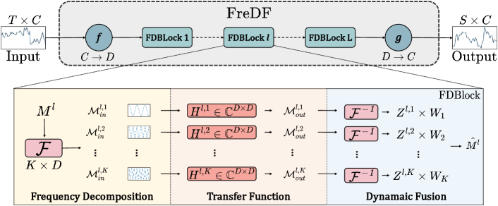
Figure 2. Overall structure of FreDF, which consists of an Embedding module $f$ for embedding the feature dimension $C$ to $D$, a Projection module $g$ for projection back to $C$, and $L$ FDBlocks. In FDBlock, we decompose and forecast in the frequency domain, and dynamically fuse the prediction results for each Fourier component.

4. Method

In this section, we begin by reformulating the TFS problem in the Fourier domain. Subsequently, we propose FreDF, a model designed to predict the output of each frequency component respectively, then combine each output using a dynamic fusion strategy. We also present theoretical evidence supporting the idea that this dynamic fusion strategy enhances the generalization ability of FreDF.

4.1. Time series forecasting in Fourier domain

To achieve effective long-term forecasting, the model must go beyond merely memorizing past data points; it needs to grasp the underlying physical rules or inherent dynamics of the observed phenomena (Luenberger, 1979). These dynamics governing the behavior of the time series, are presumed to be independent and unchanging over time (Oppenheim et al., 1997). In Fourier analysis, any time series can be represented by a set of orthogonal bases, i.e., the Fourier components; this orthogonal characteristic helps represent each rule with the dynamic of a single Fourier component (Lange et al., 2021). In this section, we assume that the time series forecasting task is under a Linear Time-invariant (LTI) condition for the independent and time-invariant property of the inherent dynamics without loss of generality.

Specifically, from (Oppenheim et al., 1997), let $x(t)\in\mathcal{I}$ be the input function and $y(t)\in\mathcal{O}$ be the output function, they are both functions of time $t$ defined in Banach space $\mathcal{I}$ and $\mathcal{O}$. The output of the LTI system can be defined as:

(1) $$y(t)=\int_{0}^{\infty}h(t-\tau)x(\tau)d\tau.$$

The goal of time-series forecasting can be regarded as finding a suitable transfer function $h:\mathcal{I}\rightarrow\mathcal{O}$.

In discrete case, the Equation 1 can be express as:

(2) $$Y[n]=h[n]*X=\sum_{m=0}^{\infty}h[n-m]X[m],$$

$X[n]$ and $Y[n]$ is the discrete form of $x(t)$ and $y(t)$, respectively, $n\in[0,1,\dots,N]$, $N$ is the length of time series, and $*$ is the convolution operator. The output series $Y=[Y[0],Y[1],\dots,Y[N]]$ are obtained by applying the convolution operator between $h$ and $X$.

The Discrete Fourier Transform (DFT) $\mathcal{F}$ (Oppenheim et al., 1999) can transform $X$ from a function of discrete time to a function of Fourier component:

(3) $$\mathcal{X}[k]=\mathcal{F}(X)[k]=\sum_{n=0}^{N-1}X[n]\cdot e^{-j\frac{2\pi}{N}kn},$$

where $j$ is the imaginary unit, $\mathcal{X}[k]$ is the $k$-th Fourier components, $k\in[0,1,\dots,K]$ and $K$ is the total number of Fourier components.

Theorem 4.1.

(The convolution theorem (Katznelson, 2004)). The convolution theorem states that the Fourier transform of a convolution of two functions equals the point-wise product of their Fourier transform:

(4) $$\mathcal{F}(h*X)[k]=\mathcal{F}(h)[k]\cdot\mathcal{F}(X)[k].$$

Applying DFT to the output sequence $Y$ according to Theorem 4.1 can convert the convolution in Equation 24 into a multiplication in the Fourier domain as:

(5) $$\mathcal{Y}[k]=\mathcal{F}(h*X)[k]=\mathcal{F}(h)[k]\cdot\mathcal{X}[k].$$

Note that $h$ is an unknown operator in the aforementioned analysis. Therefore we propose to estimate $\mathcal{F}(h)$ directly with a learnable matrix $H_{\theta}$, where $\theta$ is the parameter. The transfer process is:

(6) $$\hat{\mathcal{Y}}[k]=H_{\theta}\cdot\mathcal{X}[k],$$

where $\hat{\mathcal{Y}}$ is the estimated output in Fourier domain.

Applying inverse Discrete Fourier transform $\mathcal{F}^{-1}$ (iDFT) can convert the estimated output back to the time domain with:

(7) $$\hat{Y}[n]=\mathcal{F}^{-1}(\hat{\mathcal{Y}})=\frac{1}{N}\sum_{k=1}^{K}\hat{\mathcal{Y}}[k]\cdot e^{j\frac{2\pi}{N}kn}.$$

The learning objective for the learnable matrix is then to minimize the Mean Square Error (MSE) between the estimated output and the ground truth of the output:

(8) $$\min_{\theta}\frac{1}{N}\sum_{n=0}^{N-1}(Y[n]-\hat{Y}[n])^{2}.$$

So far, the TFS problem in the time domain has been reformulated as learning a transfer function $H_{\theta}$ in the Fourier domain.

4.2. Frequency Dynamic Fusion

Based on the findings in Section 3, there is no universal criteria to determine the importance of a specific frequency in different situations, for the role of certain frequency changes across various scenarios. For instance, a frequency may be crucial in one scenario but negatively impact performance in another. To address this variability, we propose FreDF (Frequency Dynamic Fusion), which dynamically calculates the weights for the estimated prediction of each frequency, taking their importance into account. Our proposed FreDF consists of the Embedding, the FDBlock, and the Projection layers. We provide the pseudo-code of FreDF in algorithm 1.

To predict the future $S$ timestamps, we padding $X[n]$ in time dimension with $S$ zeros as unknown data.

4.2.1. Embedding

In the Embedding module, we lift the input time series into an embedding space:

(9) $$M^{1}[n]=f(X[n]),$$

here, $M^{1}[n]$ is the embedded representation of the input time series, $f:\mathbb{R}^{C}\rightarrow\mathbb{R}^{D}$ is a multi-layer perceptron (MLP) used for the embedding, $C$ is the number of variables in the input time series, and $D$ is the dimension of the embedding space. It’s crucial to note that we are embedding the feature dimensions, not the time dimensions. This means that the transformation does not affect the temporal characteristics of the data. Therefore, subsequent operations, such as Fourier transformations that target the time dimensions, remain unaffected by the embedding process.

Algorithm 1 Pseudo-Code of FreDF

Input: Time series data $X\in\mathbb{R}^{T\times C}$, lookback length $T$, predict length $S$, variables number $C$, FDBlock number $L$, token dimension $D$, $K$ is computed as $K=\frac{T+S}{2}+1$, frequency spectrum length $K$.

1:  $X^{\prime}=$ ZeroPadTimeSeries($X$, $S$) $\triangleright$ $\mathbf{X}\in\mathbb{R}^{(T+S)\times C}$

2:  $M^{1}=$ MLP($X^{\prime}$) $\triangleright$ $M^{1}\in\mathbb{R}^{(T+S)\times D}$

3:  for $l=1$ to $L$ do

4:     for $m=1$ to $K$ do

5:        $\mathcal{M}^{l}[k]=\mathcal{F}(M^{l})[k]$ $\triangleright$ $\mathcal{M}^{l}\in\mathbb{R}^{K\times D}$

6:        for $k=1$ to $K$ do

7:           if $k\neq m$ then

8:              $\mathcal{M}^{l,m}_{in}[k]=0$

9:           else

10:              $\mathcal{M}^{l,m}_{in}[k]=\mathcal{M}^{l}[k]$

11:           end if

12:        end for

13:        Learn transfer function $H^{l,m}$ $\triangleright$ $H^{l,m}\in\mathbb{R}^{D\times D}$

14:        $\mathcal{M}^{l,m}_{out}[k]=\mathcal{M}^{l,m}_{in}[k]\cdot H^{l,m}$

15:        $Z^{l,m}=\mathcal{F}^{-1}(\mathcal{M}^{l,m}_{out})$

16:     end for

17:     $M^{l+1}=\hat{M}^{l}=\sum_{m=0}^{K}Z^{l,m}\cdot W_{m},$ $\triangleright$ $\hat{M}^{l}\in\mathbb{R}^{(T+S)\times D}$

18:  end for

19:  $\hat{Y}=MLP(\hat{M}^{L})[T:T+S,:]$

20:  return  $\hat{Y}$ $\triangleright$ Return the prediction results

Models		FreDF(Ours)		iTransformer		PatchTST		Crossformer		TiDE		TimesNet		DLinear		SCINet		FEDformer		Stationary		Autoformer
Metric		MSE	MAE	MSE	MAE	MSE	MAE	MSE	MAE	MSE	MAE	MSE	MAE	MSE	MAE	MSE	MAE	MSE	MAE	MSE	MAE	MSE	MAE
ETTm1	96	0.324	0.367	0.334	0.368	0.329	0.367	0.404	0.426	0.364	0.387	0.338	0.375	0.345	0.372	0.418	0.438	0.379	0.419	0.386	0.398	0.505	0.475
	192	0.365	0.387	0.377	0.391	0.367	0.385	0.450	0.451	0.398	0.404	0.374	0.387	0.380	0.389	0.439	0.450	0.426	0.441	0.459	0.444	0.553	0.496
	336	0.391	0.405	0.426	0.420	0.399	0.410	0.532	0.515	0.428	0.425	0.410	0.411	0.413	0.413	0.490	0.485	0.445	0.459	0.495	0.464	0.621	0.537
	720	0.459	0.436	0.491	0.459	0.454	0.439	0.666	0.589	0.487	0.461	0.478	0.450	0.474	0.453	0.595	0.550	0.543	0.490	0.585	0.516	0.671	0.561
	Avg	0.384	0.398	0.407	0.410	0.387	0.400	0.513	0.496	0.419	0.419	0.400	0.406	0.403	0.407	0.485	0.481	0.448	0.452	0.481	0.456	0.588	0.517
ETTm2	96	0.175	0.257	0.180	0.264	0.175	0.259	0.287	0.366	0.207	0.305	0.187	0.267	0.193	0.292	0.286	0.377	0.203	0.287	0.192	0.274	0.255	0.339
	192	0.241	0.299	0.250	0.309	0.241	0.302	0.414	0.492	0.290	0.364	0.249	0.309	0.284	0.362	0.399	0.445	0.269	0.328	0.280	0.339	0.281	0.340
	336	0.303	0.341	0.311	0.348	0.305	0.343	0.597	0.542	0.377	0.422	0.321	0.351	0.369	0.427	0.637	0.591	0.325	0.366	0.334	0.361	0.339	0.372
	720	0.405	0.396	0.412	0.407	0.402	0.400	1.730	1.042	0.558	0.524	0.408	0.403	0.554	0.522	0.960	0.735	0.421	0.415	0.417	0.413	0.433	0.432
	Avg	0.281	0.323	0.288	0.332	0.281	0.326	0.757	0.610	0.358	0.404	0.291	0.333	0.350	0.401	0.571	0.537	0.305	0.349	0.306	0.347	0.327	0.371
ETTh1	96	0.367	0.397	0.386	0.405	0.414	0.419	0.423	0.448	0.479	0.464	0.384	0.402	0.386	0.400	0.654	0.599	0.376	0.419	0.513	0.491	0.449	0.459
	192	0.416	0.424	0.441	0.436	0.460	0.445	0.471	0.474	0.525	0.492	0.436	0.429	0.437	0.432	0.719	0.631	0.420	0.448	0.534	0.504	0.500	0.482
	336	0.477	0.443	0.487	0.458	0.501	0.466	0.570	0.546	0.565	0.515	0.491	0.469	0.481	0.459	0.778	0.659	0.459	0.465	0.588	0.535	0.521	0.496
	720	0.478	0.458	0.503	0.491	0.500	0.488	0.653	0.621	0.594	0.558	0.521	0.500	0.519	0.516	0.836	0.699	0.506	0.507	0.643	0.616	0.514	0.512
	Avg	0.435	0.431	0.454	0.447	0.469	0.454	0.529	0.522	0.541	0.507	0.458	0.450	0.456	0.452	0.747	0.647	0.440	0.460	0.570	0.537	0.496	0.487
ETTh2	96	0.292	0.341	0.297	0.349	0.302	0.348	0.745	0.584	0.400	0.440	0.340	0.374	0.333	0.387	0.707	0.621	0.358	0.397	0.476	0.458	0.346	0.388
	192	0.376	0.391	0.380	0.400	0.388	0.400	0.877	0.656	0.528	0.509	0.402	0.414	0.477	0.476	0.860	0.689	0.429	0.439	0.512	0.493	0.456	0.452
	336	0.415	0.426	0.428	0.432	0.426	0.433	1.043	0.731	0.643	0.571	0.452	0.452	0.594	0.541	1.000	0.744	0.496	0.487	0.552	0.551	0.482	0.486
	720	0.420	0.439	0.427	0.445	0.431	0.446	1.104	0.763	0.874	0.679	0.462	0.468	0.831	0.657	1.249	0.838	0.463	0.474	0.562	0.560	0.515	0.511
	Avg	0.376	0.399	0.383	0.407	0.387	0.407	0.942	0.684	0.611	0.550	0.414	0.427	0.559	0.515	0.954	0.723	0.437	0.449	0.526	0.516	0.450	0.459
Exchange	96	0.082	0.199	0.086	0.206	0.088	0.205	0.256	0.367	0.094	0.218	0.107	0.234	0.088	0.218	0.267	0.396	0.148	0.278	0.111	0.237	0.197	0.323
	192	0.172	0.294	0.177	0.299	0.176	0.299	0.470	0.509	0.184	0.307	0.226	0.344	0.176	0.315	0.351	0.459	0.271	0.315	0.219	0.335	0.300	0.369
	336	0.316	0.405	0.331	0.417	0.301	0.397	1.268	0.883	0.349	0.431	0.367	0.448	0.313	0.427	1.324	0.853	0.460	0.427	0.421	0.476	0.509	0.524
	720	0.835	0.687	0.847	0.691	0.901	0.714	1.767	1.068	0.852	0.698	0.964	0.746	0.839	0.695	1.058	0.87	1.195	0.695	1.092	0.769	1.447	0.941
	Avg	0.351	0.396	0.360	0.403	0.367	0.404	0.940	0.707	0.370	0.413	0.416	0.443	0.354	0.414	0.750	0.626	0.519	0.429	0.461	0.454	0.613	0.539
Weather	96	0.157	0.208	0.174	0.214	0.177	0.218	0.158	0.230	0.202	0.261	0.172	0.220	0.196	0.255	0.221	0.306	0.217	0.296	0.173	0.223	0.266	0.336
	192	0.205	0.246	0.221	0.254	0.225	0.259	0.206	0.277	0.242	0.298	0.219	0.261	0.237	0.296	0.261	0.340	0.276	0.336	0.245	0.285	0.307	0.367
	336	0.259	0.287	0.278	0.296	0.278	0.297	0.272	0.335	0.287	0.335	0.280	0.306	0.283	0.335	0.309	0.378	0.339	0.380	0.321	0.338	0.359	0.395
	720	0.341	0.339	0.358	0.349	0.354	0.348	0.398	0.418	0.351	0.386	0.365	0.359	0.345	0.381	0.377	0.427	0.403	0.428	0.414	0.410	0.419	0.428
	Avg	0.241	0.270	0.258	0.279	0.259	0.281	0.259	0.315	0.271	0.320	0.259	0.287	0.265	0.317	0.292	0.363	0.309	0.360	0.288	0.314	0.338	0.382
ECL	96	0.150	0.242	0.148	0.240	0.181	0.270	0.219	0.314	0.237	0.329	0.168	0.272	0.197	0.282	0.247	0.345	0.193	0.308	0.169	0.273	0.201	0.317
	192	0.161	0.253	0.162	0.253	0.188	0.274	0.231	0.322	0.236	0.330	0.184	0.289	0.196	0.285	0.257	0.355	0.201	0.315	0.182	0.286	0.222	0.334
	336	0.176	0.268	0.178	0.269	0.204	0.293	0.246	0.337	0.249	0.344	0.198	0.300	0.209	0.301	0.269	0.369	0.214	0.329	0.200	0.304	0.231	0.338
	720	0.217	0.311	0.225	0.317	0.246	0.324	0.280	0.363	0.284	0.373	0.220	0.320	0.245	0.333	0.299	0.390	0.246	0.355	0.222	0.321	0.254	0.361
	Avg	0.176	0.268	0.178	0.270	0.205	0.290	0.244	0.334	0.251	0.344	0.192	0.295	0.212	0.300	0.268	0.365	0.214	0.327	0.193	0.296	0.227	0.338
Solar-Energy	96	0.214	0.247	0.203	0.237	0.234	0.286	0.310	0.331	0.312	0.399	0.250	0.292	0.290	0.378	0.237	0.344	0.242	0.342	0.215	0.249	0.884	0.711
	192	0.230	0.255	0.233	0.261	0.267	0.310	0.734	0.725	0.339	0.416	0.296	0.318	0.320	0.398	0.280	0.380	0.285	0.380	0.254	0.272	0.834	0.692
	336	0.242	0.266	0.248	0.273	0.290	0.315	0.750	0.735	0.368	0.430	0.319	0.330	0.353	0.415	0.304	0.389	0.282	0.376	0.290	0.296	0.941	0.723
	720	0.245	0.271	0.249	0.275	0.289	0.317	0.769	0.765	0.370	0.425	0.338	0.337	0.356	0.413	0.308	0.388	0.357	0.427	0.285	0.295	0.882	0.717
	Avg	0.232	0.259	0.233	0.262	0.270	0.307	0.641	0.639	0.347	0.417	0.301	0.319	0.330	0.401	0.282	0.375	0.291	0.381	0.261	0.381	0.885	0.711
$1^{\text{st}}$ Count		34	36	2	2	3	2	0	0	0	0	0	0	0	0	0	0	1	0	0	0	0	0

Table 1. Long-term multivariate forecasting results with prediction lengths $S\in\left\{96,192,336,720\right\}$ and fixed lookback length $T=96$. The best Forecasting results in bold and the second underlined. The lower MSE/MAE indicates the more accurate prediction result.

4.2.2. FDBlocks

Within each FDBlock, we apply Fast Fourier Transform (FFT)(Nussbaumer and Nussbaumer, 1982) to the input embedding $M^{l}[n]$, transforming it into the Fourier domain, which is an efficient algorithm to perform DFT:

(10) $$\mathcal{M}^{l}[k]=\mathcal{F}(M^{l})[k],$$

here $\mathcal{M}^{l}[k]$ is the Fourier components, $l=1,2,\dots,L$ denotes the $l$-th FDBlock and $L$ is the total number of FDBlocks.

To facilitate independent processing, we propose a decoupling strategy. Instead of treating the Fourier components $\mathcal{M}^{l}[k]\in\mathbb{C}^{K\times D}$ as a whole, we create $K$ copies of each frequency component and only retain the $m$-th frequency in $m$-th copy, denoted as $\mathcal{M}^{l,m}_{in}[k]$:

(11) $$\mathcal{M}^{l,m}_{in}(k)=\left\{\begin{array}[]{ll}0&\text{if }k\neq m\\ \mathcal{M}^{l}(k)&\text{if }k=m\end{array},k=0,1,...,K.\right.$$

This strategy allows us to maintain the original dimensionality of the data while enabling independent processing of each frequency. Next, based on subsection 4.1, we aim to learn transfer functions $H^{l,m}\in\mathbb{C}^{D\times D}$, $m\in[1,\dots,K]$for each independent component $\mathcal{M}^{l,m}_{in}=\mathcal{M}^{l}[m]$, $m\in[1,\dots,K]$, and obtain the estimated output $\mathcal{M}^{l,m}_{out}$ in the Fourier domain with:

(12) $$\mathcal{M}^{l,m}_{out}=\mathcal{M}^{l,m}_{in}\cdot H^{l,m}.$$

The estimated output for frequency $m$ in the time domain $Z^{l,m}[n]$ can be obtained by applying inverse Fast Fourier Transform (iFFT) to $\mathcal{M}^{l,m}_{out}$. The result of this operation is represented as:

(13) $$Z^{l,m}[n]=\mathcal{F}^{-1}(\mathcal{M}^{l,m}_{out})[n].$$

So far, we have decomposed the prediction process of each individual frequency $m$.

Next, we apply a trainable weight vector $W\in\mathbb{R}^{K}$, where each component $W_{m}$ represents the importance of the $m$-th frequency when predicting the output embedding. The estimated output $\hat{M}^{l}[n]$ is then represented as a weighted sum of all the individual frequency predictions $Z^{l,m}[n]$, with each prediction multiplied by its corresponding weight $W_{m}$. The estimated output $\hat{M}^{l}[n]$ is represented as a weighted sum of all the individual frequency predictions $Z^{l,m}[n]$, as given by the following equation:

(14) $$\hat{M}^{l}[n]=\sum_{m=0}^{K}Z^{l,m}[n]\cdot W_{m},$$

where prediction $Z^{l,m}[n]$ is multiplied by its corresponding weight $W_{m}$ and $W_{m}$ can be either static or dynamic, i.e. fixed or learnable.

The FDBlock is formulated as an iterative architecture, where output $\hat{M}^{l}[n]$ of the $l$-th layer serves as input of the $(l+1)$-th layer.

During the training process, we aim to learn the transfer functions $H^{l,m}\in\mathbb{C}^{D\times D}$ and the weight vector $W\in\mathbb{R}^{K}$ by minimizing a loss function, which measures the difference between the estimated output $\hat{Y}[n]$ and the true output $Y[n]$.

4.2.3. Projection

After $L$ FDBlocks, we apply another MLP $g:\mathbb{R}^{D}\rightarrow\mathbb{R}^{C}$ to the final estimated output $\hat{M}^{L}[n]$, projecting it back to the variable space. The result of this operation is represented as:

(15) $$\hat{Y}[n]=g(\hat{M}^{L}[n])[T:T+S,:].$$

4.3. Theoretical Analysis

In this subsection, we provide a theoretical analysis to demonstrate the effectiveness of our dynamic fusion method. Without loss of generality, time series forecasting methods could be regarded as auto-regressive models (Box et al., 2015), from this perspective, we indicate that the generalization ability of time series prediction models could be reflected in the following two aspects: the capacity to capture the long-term dependency of time series, as well as the capacity to achieve good prediction results in different scenarios.

For simplicity, consider the fusion strategy in a regression setting using a mean squared loss function. Firstly, we propose to characterize the generalization error bound using Rademacher complexity (Bartlett et al., 2003) and separate the bound into three components (Theorem 4.2). Meanwhile, we also give further proof based on the above separation to illustrate that the dynamic fusion method achieves a better ability to capture long-term dependency under certain conditions (Theorem 4.3). Secondly, we demonstrate that the quantity of parameters in our method is fewer than compared methods, which indicates that our method is more flexible to apply to more scenarios, experiment results in Section 5.2 also validate our illustration as well. See Appendix A for details.

Specifically, we use $\mathcal{X}$, $\mathcal{Y}$, and $\mathcal{Z}$ to denote the input space (historical sequence), target space (prediction sequence), and latent space. Define $u:\mathcal{X}\xrightarrow{}\mathcal{Z}$ is a fusion mapping from the input space to the latent space, $g:\mathcal{Z}\xrightarrow{}\mathcal{Y}$ is a task mapping. Our goal is to learn the fusion operator $f=g\circ{}u(x)$, which is essentially a regression model. Under an $H$ frequency components scenario, $f^{h}$ is the frequency-specific composite function of frequency component $x^{h}$. The final prediction of the dynamic fusion method is calculated by: $f(x)=\sum_{h=1}^{H}w^{h}\cdot f^{h}(x^{h})$, where $f(x)$ denotes the final prediction. In contrast to static fusion, i.e., every frequency is given a predefined weight which is a constant, dynamic fusion calculates the weights of every frequency dynamically. To distinguish them, denotes $w_{static}^{h}$ the weight of frequency $h$ in static situation and $w_{dynamic}^{h}$ the weight of frequency $h$ in dynamic situation. The generalization error of regression model $f$ is defined as:

(16) $$\mathrm{GError}=\mathbb{E}_{(x,y)\sim\mathcal{D}}[l(f(x),y)],$$

where $\mathcal{D}$ is the unknown joint distribution, $l$ is mean squared loss function. Conveniently, we simplify the regression loss $l(f^{h}(x^{h}),y)$ as $l^{h}$. Now we present the first main result of frequency fusion.

Theorem 4.2.

Given the historical sequence $X_{T}\in\mathbb{R}^{T\times C}$ and the ground truth of prediction sequence $Y_{T^{\prime}}\in\mathbb{R}^{T^{\prime}\times C}$, $\hat{E}(f^{h})$ is the empirical error of $f^{h}$ on frequency $h$. Then for any hypothesis $f$ in the finite set $F$ and $1\textgreater\delta\textgreater 0$, with probability at least $1-\delta$, it holds that

(17) $$\begin{split}\mathrm{GError}\leq\sum_{h=1}^{H}\mathbb{E}(w^{h})\hat{E}(f^{h})+\sum_{h=1}^{H}\mathbb{E}(w^{h})\mathfrak{R}_{h}(f^{h})\\ +\sum_{h=1}^{H}Cov(w^{h},l^{h})+M\sqrt{\frac{ln(1/\delta)}{2H}},\end{split}$$

where $\mathbb{E}(w^{h})$ represents the expectations of fusion weights on joint distribution $\mathcal{D}$, $\mathfrak{R}_{h}(f^{h})$ represents Rademacher complexity, and $Cov(w^{h},l^{h})$ represents covariance between fusion weight and loss.

Theorem 4.2 demonstrates that the generalization error of the regression model is bounded by the weighted average performances of all regression operators for each frequency in terms of empirical loss, model complexity, and the covariance between fusion weight and regression loss of all frequencies. Next, we aim to confirm whether dynamic fusion offers a tighter general error bound than static fusion. Informally, in Equation 17, the covariance term measures the joint variability of $w^{h}$ and $l^{h}$. However, in static fusion, $w_{static}^{h}$ is a constant, which means that the covariance is equal to zero for any static fusion method. Thus the generalization error bound of static fusion methods is reduced to:

(18) $$\mathrm{GError}(f_{static}) \leq\sum_{h=1}^{H}(w_{static}^{h})\hat{E}(f^{h})$$

$$+ \sum_{h=1}^{H}(w_{static}^{h})\mathfrak{R}_{h}(f^{h})+M\sqrt{\frac{ln(1/\delta)}{2H}}.$$

So when the summation of the average empirical loss, the average complexity is invariant or smaller in dynamic fusion and the covariance is no greater than zero, we can ensure that dynamic fusion provably outperforms static fusion. This theorem is formally presented as:

Theorem 4.3.

Let $\overline{\mathrm{GError}}(f_{dynamic})$, $\overline{\mathrm{GError}}(f_{static})$ be the upper bound of generalization regression error of dynamic and static fusion method respectively. $\hat{E}(f^{h})$ is the empirical error defined in Theorem 4.2. Then for any hypothesis $f_{dynamic}$, $f_{static}$ in finite set $F$ and $1\textgreater\delta\textgreater 0$, it holds that

(19) $$\overline{\mathrm{GError}}(f_{dynamic})\leq\overline{\mathrm{GError}}(f_{static})$$

with probability at least $1-\delta$, if we have

(20) $$\mathbb{E}(w_{dynamic}^{h})=w_{static}^{h}$$

and

(21) $$r(w_{dynamic}^{h},l^{h})\leq 0$$

for all frequencies, where $r$ is the Pearson correlation coefficient which measures the correlation between fusion weights $w_{dynamic}^{h}$ and the loss of each frequency $l^{h}$.

Theorem 4.2 and Theorem 4.3 verify that the dynamic fusion method has a lower generalization bound, which indicates the capacity to capture the long-term dependency of our method. Furthermore, suppose for each frequency, the regression operator used in dynamic and static fusion are of the same architecture, then the intrinsic complexity $\mathfrak{R}_{h}(f^{h})$ can be invariant. Thus, it holds that

(22) $$\sum_{h=1}^{H}\mathbb{E}(w_{dynamic}^{h})\mathfrak{R}_{h}(f^{h})\leq\sum_{h=1}^{H}(w_{static}^{h})\mathfrak{R}_{h}(f^{h}).$$

In Equation 22, it is easy to derive the conclusion that our model has a lower average complexity, corresponding to a lower quantity of parameters during the training process. Experiment results in Section 5.2 also validate this conclusion.

5. Experiments

In this section, we first provide the details of the implementation and datasets. Next, we present the comparison results on eight benchmark datasets. Lastly, we conduct ablation studies to evaluate the effectiveness of each module in our method.

Table 2. Ablation on the influence of transfer function.

Methods	Metric	ETTh1				ETTm1				Exchange-rate
		96	192	336	720	96	192	336	720	96	192	336	720
W Transfer function	MSE	0.367	0.416	0.477	0.478	0.324	0.365	0.391	0.459	0.082	0.172	0.316	0.835
	MAE	0.397	0.424	0.443	0.458	0.367	0.387	0.405	0.436	0.199	0.294	0.405	0.687
W/O Transfer function	MSE	0.439	0.492	0.529	0.522	0.378	0.421	0.441	0.518	0.129	0.218	0.254	0.897
	MAE	0.444	0.505	0.561	0.541	0.405	0.432	0.439	0.487	0.251	0.344	0.312	0.709

5.1. Main Results

We thoroughly evaluate the proposed FreDF on various long-term time series forecasting benchmarks. For better comparison, we follow the experiment settings of iTransformer in (Liu et al., 2023a) the prediction lengths for both training and evaluation vary within the set $S\in\{96,192,336,720\}$, with a fixed lookback length of $T=96$.

5.1.1. Baselines

We carefully choose 10 well-acknowledged forecasting models as our benchmark, including (1) Transformer-based methods: iTransformer (Liu et al., 2023a), Autoformer (Wu et al., 2021), FEDformer (Zhou et al., 2022b), Stationary (Liu et al., 2022a), Crossformer (Zhang and Yan, 2023), PatchTST (Nie et al., 2023); (2) Linear-based methods: DLinear (Zeng et al., 2023), TiDE (Das et al., 2023); and (3) TCN-based methods: SCINet (Liu et al., 2022b), TimesNet (Wu et al., 2023).

5.1.2. Forecasting Results

Table 1 presents the results of FreDF in long-term multivariate forecasting with the best in bold and the second underlined. The lower MSE/MAE indicates the more accurate prediction result. Results demonstrate that our model performs optimally in 70 out of 80 benchmarks. Compared to FEDformer (Zhou et al., 2022b), FreDF shows an average improvement of $13\%$ in terms of MSE and MAE, reaching up to $33\%$ improvement on the Exchange-rate dataset. Compared to the best-performing Transformer-based model:iTransformer (Liu et al., 2023a), FreDF consistently achieves superior performance across almost all datasets.

Table 3. Ablation between static fusion and dynamic fusion.

Models		FreDF		FreSF
Metric		MSE	MAE	MSE	MAE
Weather	96	0.153	0.199	0.175	0.239
	192	0.205	0.246	0.215	0.276
	336	0.259	0.587	0.263	0.312
	720	0.341	0.339	0.343	0.377
Exchange	96	0.082	0.199	0.129	0.239
	192	0.172	0.294	0.231	0.332
	336	0.316	0.405	0.360	0.451
	720	0.835	0.687	0.891	0.741
ETTh1	96	0.367	0.397	0.428	0.437
	192	0.416	0.424	0.475	0.456
	336	0.477	0.443	0.509	0.477
	720	0.478	0.458	0.509	0.490
ETTm1	96	0.324	0.367	0.369	0.401
	192	0.365	0.387	0.419	0.430
	336	0.391	0.405	0.440	0.438
	720	0.459	0.436	0.497	0.468

5.2. Ablation Study

In this section, we conduct ablation studies to examine the influence of transfer functions, dynamic fusion mechanisms, and the number of parameters in the proposed FreDF.

5.2.1. Influence of transfer function

We conduct an ablation study about the influence of the transfer function. We remove the transfer function in FreDF as the control group, follow the setup in Section 5.1, and carry out predictions on the ETTh1, ETTm1, and Exchange-rate dataset. We present the results in Table 2, which illustrates the crucial role of the transfer function and confirms the correctness of our analysis in Section 4.1.

5.2.2. Influence of dynamic fusion

We conduct an ablation study to investigate the influence of dynamic fusion. We replace the learnable weight vector with a fixed weight vector and name this modified model FreSF. Predictions are carried out on the ETT(ETTh1, ETTh2, ETTm1, ETTm2), Weather, and Exchang-rate datasets using the setup outlined in Section 5.1. The results are presented in Table LABEL:tab:ab2. Additionally, we visualize the prediction results (with a prediction length $S=96$) for both FreSF and FreDF in Appendix D. The experimental results demonstrate the effectiveness of the dynamic fusion strategy.

Table 4. Comparison of the number of parameters.

Models	Ours	iTransformer	PatchTST	FEDformer	FiLM
params	151.4K	3.1M	3.5M	14.0M	12.0M

5.2.3. Number of parameters

We use iTransformer (Liu et al., 2023a), patchTST (Nie et al., 2023), FEDformer (Zhou et al., 2022b) and FiLM (Zhou et al., 2022a) for comparison, and calculate the number of model parameters when forecasting the same task, present the results in Table 4. Our model despite using a relatively small number of parameters, can achieve good accuracy in prediction tasks. This also validates the superiority of our model, which is consistent with the theoretical analysis in Section 4.3.

6. Conclusion

In this paper, we experimentally explore the different roles of frequency in various scenarios. To better utilize these distinctions, we reformulate the problem of time series forecasting as learning transfer functions in the Fourier domain and design the FreDF model, which can independently forecast each Fourier component and dynamically fuse outputs from different frequencies. Then, we provide a novel understanding of the generalization ability of time series forecasting. Further, we also propose the generalization bound for time series forecasting and demonstrate that FreDF has a lower generalization bound, indicating its better generalization ability. Extensive experiments validate the effectiveness of FreDF on multiple benchmark datasets.

The Appendix provides supplementary information and additional details that support the primary discoveries and methodologies proposed in this paper. It is organized into several sections: Appendix A contains the proof of Theorem 2 and Theorem 3.

Appendix A Proofs

In this section, we will prove Theorem 2 and Theorem 3, which is used for the theoretical analysis.

A.1. Proof of Theorem 2

Note that $l$ is a convex regression loss function, which indicates that

(23) $$l(f(x),y)=l(\sum_{h=1}^{H}w^{h}f^{h}(x^{h}),y)\leq\sum_{h=1}^{H}w^{h}l(f^{h}(x^{h}),y)$$

Then we take the expectation on both sides of the above equation

(24) $$\mathbb{E}_{(x,y)\sim D}l(f(x),y)\leq\mathbb{E}_{(x,y)\sim D}\sum_{h=1}^{H}(w^{h}l(f^{h}(x^{h}),y)),$$

since expectation is a linear operator and the expected value of the product is equal to the product of the expected values plus the covariance, we can further decompose the right-hand side of the equation into

(25) $$\mathbb{E}_{(x,y)\sim D}l(f,y)\leq\sum_{h=1}^{H}\mathbb{E}_{(x,y)\sim D}[w^{h}l(f^{h},y)]$$

$$=\sum_{h=1}^{H}\mathbb{E}_{(x,y)\sim D}(w^{h})\mathbb{E}_{(x,y)\sim D}(l(f^{h},y))$$

$$+Cov(w^{h},l(f^{h},y))$$

Next, we recap the Rademacher complexity measure for model complexity. We use complexity based learning theory to quantify the generalization error of the proposed model.

Given the historical sequence and the ground truth of the prediction sequence, $\hat{E}(f^{h})$ is the empirical error of $f^{h}$. Then for any hypothesis $f$ in the finite set $F$ and $1\textgreater\delta\textgreater 0$, with probability at least $1-\delta$, we have

(26) $$\mathbb{E}_{(x,y)\sim D}(f^{h})\leq\hat{E}(f^{h})+\mathfrak{R}_{h}(F)+\sqrt{\frac{ln(1/\delta)}{2H}}$$

where $\mathfrak{R}_{h}(F)$ is the Rademacher complexities.

Finally, it holds with probability at least $1-\delta$ that

(27) $$\begin{split}\mathrm{GError}(f)\leq\sum_{h=1}^{H}\mathbb{E}(w^{h})\hat{E}(f^{h})+\mathbb{E}(w^{h})\mathfrak{R}_{h}(f^{h})\\ +Cov(w^{h},l(f^{h},y)+M\sqrt{\frac{ln(1/\delta)}{2H}}.\end{split}$$

A.2. Proof of Theorem 3

Let $\overline{\mathrm{GError}}(f_{dynamic})$, $\overline{\mathrm{GError}}(f_{static})$ be the upper bound of the generalization regression error of dynamic and static fusion method, respectively. $\hat{E}(f^{h})$ is the empirical error defined in Theorem 1. Theoretically, optimizing over the same function class results in the same empirical risk. Therefore,

(28) $$\hat{E}(f_{static}^{h})=\hat{E}(f_{dynamic}^{h})$$

Additionally, the intrinsic complexity is also invariant

(29) $$\mathfrak{R}_{h}(f_{static}^{h})=\mathfrak{R}_{h}(f_{dynamic}^{h}).$$

Thus in this special case, it holds that

(30) $$\sum_{h=1}^{H}\mathbb{E}(w_{dynamic}^{h})\hat{E}(f^{h})\leq\sum_{h=1}^{H}(w_{static}^{h})\hat{E}(f^{h}),$$

and

(31) $$\sum_{h=1}^{H}\mathbb{E}(w_{dynamic}^{h})\mathfrak{R}_{h}(f^{h})\leq\sum_{h=1}^{H}(w_{static}^{h})\mathfrak{R}_{h}(f^{h}).$$

if $\mathbb{E}(w_{dynamic}^{h})=w_{static}^{h}$.

Since the covariance and the correlation coefficient have the same sign, when $r(w^{h},l^{h})\leq 0$, the covariance $Cov(w^{h},l^{h})$ is also less than or equal to zero. Therefore, it holds that

(32) $$\overline{\mathrm{GError}}(f_{dynamic})\leq\overline{\mathrm{GError}}(f_{static})$$

with probability at least $1-\delta$, if we have

(33) $$\mathbb{E}(w_{dynamic}^{h})=w_{static}^{h}$$

and

(34) $$r(w_{dynamic}^{h},l(f^{h}))\leq 0$$

for all frequencies $h$.

Appendix B Implement Details

All the experiments are implemented in PyTorch (Paszke et al., 2019) and trained on NVIDIA V100 32GB GPUs. We use ADAM (Kingma and Ba, 2015) with an initial learning rate in $\{10^{-3},10^{-4}\}$ and MSELoss for model optimization. An early stopping counter is employed to stop the training process after three epochs if no loss degradation on the valid set is observed. The mean square error (MSE) and mean absolute error (MAE) are used as metrics. All experiments are repeated 3 times and the mean of the metrics is used in the final results. The transfer function is implemented using the complex 64 data type in PyTorch. The batch size is set to 4 and the number of training epochs is set to 10. We set the number of FDBlocks in our proposed model $L\in\left\{1,2,3\right\}$. The dimension of series representations $D\in\left\{64,128,256,512\right\}$, or it is not embedded at all. We set the dropout rates in $\left\{0,0.2,0.4\right\}$.

Table 5. Detailed dataset descriptions. Dim denotes the variate number of each data set. Dataset Size denotes the total number of time points in (Train, Validation, Test) split, respectively. Prediction Length denotes the future time points to be predicted, and four prediction settings are included in each data set. Frequency denotes the sampling interval of time points.

Dataset	Dim	Prediction Length	Dataset Size	Frequency	Information
ETTh1,ETTh2	7	{96, 192, 336, 720}	(8545, 2881, 2881)	Hourly	Electricity
ETTm1,ETTm2	7	{96, 192, 336, 720}	(34465, 11521, 11521)	15min	Electricity
Exchange	8	{96, 192, 336, 720}	(5120, 665, 1422)	Daily	Economy
Weather	21	{96, 192, 336, 720}	(36792, 5271, 10540)	10min	Weather
ECL	321	{96, 192, 336, 720}	(18317, 2633, 5261)	Hourly	Electricity
Solar-Energy	137	{96, 192, 336, 720}	(36601, 5161, 10417)	10min	Energy

Appendix C Dataset Descriptions

In this paper, we conducted tests using eight real-world datasets. These datasets include:

• ETT contains two sub-datasets: ETT1 and ETT2, collected from two electricity transformers at two stations. Each of them has two versions in different resolutions (15 minutes and 1h). ETT dataset contains multiple series of loads and one series of oil temperatures.

• Weather covers 21 meteorological variables recorded at 10-minute intervals throughout the year 2020. The data was collected by the Max Planck Institute for Biogeochemistry’s Weather Station, providing valuable meteorological insights.

• Exchange-rate, which contains daily exchange rate data spanning from 1990 to 2016 for eight countries. It offers information on the currency exchange rates across different time periods.

• ECL contains the electricity consumption of 370 clients for short-term forecasting while it contains the electricity consumption of 321 clients for long-term forecasting. It is collected since 01/01/2011. The data sampling interval is every 15 minutes.

• Solar-Energy is about the solar power collected by the National Renewable Energy Laboratory. We choose the power plant data points in Florida as the data set which contains 593 points. The data is collected from 01/01/2006 to 31/12/2016 with the sampling interval of every 1 hour.

We follow the same data processing and train-validation-test set split protocol used in iTransformer, where the train, validation, and test datasets are strictly divided according to chronological order to make sure there are no data leakage issues. As for the forecasting settings, the lookback length is set to 96, while their prediction length varies in $\{96,192,336,720\}$. The details of the datasets are provided in Table 5.

Appendix D Influence of dynamic fusion

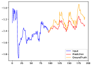
(a) FreSF on ETTh1

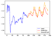
(b) FreDF on ETTh1

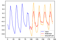
(c) FreSF on ETTh2

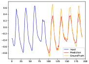
(d) FreDF on ETTh2

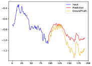
(e) FreSF on ETTm1

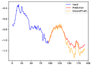
(f) FreDF on ETTm1

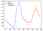
(g) FreSF on ETTm2

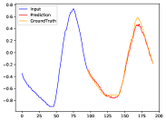
(h) FreDF on ETTm2

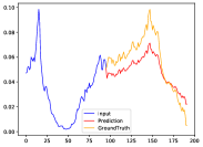
(i) FreSF on Weather

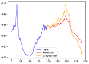
(j) FreDF on Weather

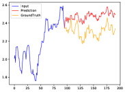
(k) FreSF on Exchange-rate

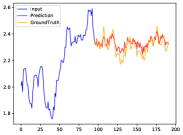
(l) FreDF on Exchange-rate

Figure 3. Visualization comparing FreSF and FreDF.

We conduct an ablation study to investigate the influence of dynamic fusion. We replace the learnable weight vector with a fixed weight vector and name this modified model FreSF. Predictions are carried out on the ETT(ETTh1, ETTh2, ETTm1, ETTm2), Weather, and Exchang-rate datasets. We visualize the prediction results (with a prediction length $S=96$) for both FreSF and FreDF in Figure 3. In the ETTh1 and ETTm1 datasets, static fusion manages to capture the overall trends and detailed shifts, but the predicted values deviate significantly from the actual figures. This issue can be effectively addressed by employing dynamic fusion. Similarly, in the ETTh2 and ETTm2 datasets, static fusion’s predictions are not quite accurate at the extreme points, a problem that dynamic fusion can effectively solve. Likewise, when dynamic fusion is applied to the Weather and Exchange-rate datasets, the prediction curve aligns more closely with the ground truth.

Appendix E Ablation on the influence of operation sequence

We conduct an ablation study about the influence of operation sequence. Our model initially conducts an inverse fast Fourier transform(iFFT) on the spectrum $\mathcal{M}^{l,m}_{out}$ obtained from the transfer function for each frequency $\mathcal{M}^{l,m}_{in}$. We then dynamically fusion the predicted results $Z^{l,m}$ for each frequency. In this section, we first dynamically fuse the spectrums $\mathcal{M}^{l,m}_{out}$ obtained from the transfer function for each frequency, followed by an iFFT on the result of this fusion. We prevent the result in Table 6

Table 6. Ablation on the influence of operation sequence.

Methods	Metric	Weather				ECL				Exchange-rate
		96	192	336	720	96	192	336	720	96	192	336	720
Dynamic Fusion on $Z^{l,m}$ (Our)	MSE	0.157	0.205	0.259	0.341	0.150	0.161	0.176	0.217	0.082	0.172	0.316	0.835
	MAE	0.208	0.246	0.287	0.339	0.242	0.253	0.268	0.311	0.199	0.294	0.405	0.687
Dynamic Fusion on spectrums $\mathcal{M}^{l,m}_{out}$	MSE	0.161	0.209	0.262	0.345	0.154	0.163	0.176	0.221	0.083	0.174	0.318	0.839
	MAE	0.214	0.253	0.292	0.347	0.242	0.253	0.270	0.313	0.199	0.295	0.406	0.670

Appendix F Ablation on the influence of FDBlock number: $L$

To further figure out the impact of different numbers of FDBlock, we perform experiments with three different $L$ ranging from 1 to 3. As shown in Table 7. And $L=1$ is a generally good choice.

Table 7. Ablation on the number of FDBlock.

FDBlock		ETTh2		ETTm2		Weather
Metric		MSE	MAE	MSE	MAE	MSE	MAE
$L=1$	96	0.292	0.341	0.175	0.257	0.157	0.208
	192	0.376	0.391	0.242	0.300	0.205	0.246
	336	0.419	0.428	0.303	0.341	0.260	0.287
	720	0.420	0.439	0.405	0.396	0.341	0.339
$L=2$	96	0.295	0.342	0.176	0.257	0.157	0.209
	192	0.377	0.390	0.241	0.300	0.206	0.246
	336	0.415	0.426	0.304	0.343	0.259	0.287
	720	0.422	0.440	0.406	0.398	0.342	0.339
$L=3$	96	0.293	0.341	0.176	0.258	0.158	0.208
	192	0.378	0.394	0.241	0.299	0.207	0.248
	336	0.416	0.426	0.304	0.345	0.262	0.289
	720	0.421	0.440	0.407	0.397	0.343	0.340

Appendix G Motivation Experiments

We present the full results of motivation experiments in Table 8. After eliminating low-frequency, we observe enhanced accuracy in the ETTm2 and ETTh2 datasets. Similarly, eliminating mid-frequency signals led to improved results in the ETTh2 and Exchange-rate datasets. The elimination of high-frequency results in more precise results in ETTh1, ETTm2, ETTh1, ETTh2, Exchange-rate, and weather datasets. The most significant improvement is seen when eliminating high-frequency signals. Nevertheless, removing low-frequency and mid-frequency signals can also improve prediction performance on some datasets.

Appendix H Compared with model that discards high frequencies

We follow FITS (Xu et al., 2024) to grid search on the look-back window of $S\in\left\{90,180,360,720\right\}$ and compare forecasting performance using Mean Squared Error (MSE). The results in Table 9 demonstrate the correctness of our different treatments for different frequencies.

Appendix I Compared with model that treats all frequencies equally

We follow FreTS (Yi et al., 2023c) to normalize them with the min-max normalization and compare forecasting performance using Mean Absolute Error (MAE). The results in Table 10 demonstrate the correctness of our different treatments for different frequencies.

Appendix J Lookback Window: ModernTCN vs Us

At the 2024 International Conference on Learning Representations (ICLR), a groundbreaking approach, ModernTCN, was presented for time series forecasting. However, it’s worth mentioning that the lookback window length used in their study consistently surpasses 96. In our case, all experiments utilize a lookback window length of 96, which makes a direct comparison not feasible.

Table 8. The comparison of prediction results using different frequencies on six datasets. The best Forecasting results in bold. The lower MSE/MAE indicates the more accurate prediction result.

Models	W all frequency		W/O low-frequency		W/O mid-frequency		W/O high-frequency
Metric	MSE	MAE	MSE	MAE	MSE	MAE	MSE	MAE
ETTm1	0.0221	0.0954	0.0839	0.1827	0.0723	0.1683	0.0116	0.0583
ETTm2	0.0601	0.1544	0.0185	0.0850	0.0852	0.1468	0.0511	0.1149
ETTh1	0.0475	0.1352	0.1333	0.2351	0.0543	0.1432	0.0409	0.1193
ETTh2	0.5288	0.4734	0.2559	0.3178	0.1396	0.2217	0.1041	0.1848
Exchange	0.0436	0.1218	0.0482	0.1292	0.0156	0.0745	0.0157	0.0733
Weather	0.0011	0.0217	0.0015	0.0207	0.0041	0.0379	0.0011	0.0186

Table 9. Compare FreDF with FITS.

Dataset	ETTh1				ETTm1				ECL
Horizon	96	192	336	720	96	192	336	720	96	192	336	720
FITS	0.372	0.404	0.427	0.424	0.303	0.337	0.366	0.415	0.134	0.149	0.165	0.203
FreDF	0.351	0.395	0.409	0.412	0.291	0.319	0.352	0.408	0.126	0.138	0.151	0.196

Table 10. Compare FreDF with FreTS.

Dataset	ECL				Weather				Exchange
Horizon	96	192	336	720	96	192	336	720	96	192	336	720
FreTS	0.039	0.040	0.046	0.052	0.032	0.040	0.046	0.055	0.037	0.050	0.062	0.088
FreDF	0.032	0.034	0.042	0.049	0.028	0.035	0.042	0.049	0.032	0.048	0.059	0.084