Modified gravity in the presence of matter creation in the late Universe: alleviation of the Hubble tension

Abstract

We consider a dynamic scenario for characterizing the late Universe evolution, aiming to mitigate the Hubble tension. Specifically, we consider a metric $f(R)$ gravity in the Jordan frame which is implemented to the dynamics of a flat isotropic Universe. This cosmological model incorporates a matter creation process due to the time variation of the cosmological gravitational field. We model particle creation by representing the isotropic Universe (specifically, a given fiducial volume) as an open thermodynamic system. The resulting dynamical model involves four unknowns: the Hubble parameter, the non-minimally coupled scalar field, its potential, and the energy density of the matter component. We impose suitable conditions to derive a closed system for these functions of the redshift. In this model, the vacuum energy density of the present Universe is determined by the scalar field potential, in line with the modified gravity scenario. Hence, we construct a viable model, determining the form of the $f(R)$ theory a posteriori and appropriately constraining the phenomenological parameters of the matter creation process to eliminate tachyon modes. Finally, by analyzing the allowed parameter space, we demonstrate that the Planck evolution of the Hubble parameter can be reconciled with the late Universe dynamics, thus alleviating the Hubble tension.

I Introduction

Over the past decade, cosmological studies of the late Universe have uncovered a significant discrepancy in data, known as the “Hubble tension”. This tension arises from the differing values of the Hubble constant ($H_{0}$) measured by the SH0ES Collaboration using Type Ia Supernova (SNIa) data Scolnic_2022 ; 2018ApJ…859..101S ; Brout:2022vxf ; riess2022apjl and those obtained by the Planck Satellite Collaboration Planck:2018vyg . The discrepancy, approximately $5\sigma$, presents a perplexing challenge, prompting new considerations regarding the dynamics of the late Universe. For a series of discussions on this topic, see schiavone_mnras ; deangelis-fr-mnras ; 2024PDU….4401486M ; 2024PhRvD.109b3527A ; Nojiri:2022ski ; Odintsov:2020qzd ; 2016RPPh…79i6901W ; naidoo2024PhRvD . The possibility of interpreting the Hubble tension as a continuous effective variation of the Hubble constant based on redshift — where its value appears to depend on the redshift region of the astrophysical sources used for its determination — has been supported by analyses in apj-powerlaw ; galaxies10010024 ; 2024MNRAS.530.5091X , and also discussed in Krishnan:2020vaf ; kazantzidis . Moreover, the coexistence of SNIa and Baryonic Acoustic Oscillations (BAO) 2021MNRAS.505.3866E (and references therein) data within the same redshift region, and their resulting tension, as BAO provides a $H_{0}$ value compatible with that from Planck, has led to the development of early dark energy (DE) models giare2024arXiv240412779G and a suitable combination of early and late modified dynamics 2023Univ….9..393V ; 2020PhRvD.102b3518V . In particular, the analysis in deangelis-fr-mnras proposed a specific $f(R)$ model, examined within the so-called Jordan frame Sotiriou-Faraoni:2010 ; NOJIRI201159 , to effectively address the Hubble tension in the presence of evolutionary DE, which transits to a phantom contribution at $z>1$. This model presents an intriguing scenario where the Hubble tension is essentially resolved at $z\gtrsim 2$ since the non-minimally coupled scalar field shows a monotonically increasing behavior toward an asymptote. This asymptotic configuration aligns with the Planck value for the Hubble constant, occurring at a relatively low redshift.

In the present study, we explore a similar approach, but instead of positing the existence of evolutionary DE from the outset, we consider a more natural physical scenario. This scenario involves the gravitational field generating weakly massive particles due to its time variation, effectively introducing a radiation component in the late Universe. In particular, the matter creation process is treated on a phenomenological level, by regarding the Universe as an open thermodynamic system like in 2001CQGra..18..193M ; 1992PhLA..162..223C , and the particle creation rate is determined via an ansatz having the form of a power-law in the Hubble parameter (for a different approach to matter creation by a scalar field see erdem24a ). After constructing the dynamical system that governs the late Universe dynamics and incorporating the creation of a radiation component by the gravitational background, we show how the Hubble tension can be properly attenuated in certain favoured regions of the parameter space. The resulting framework thus presents a promising depiction of the underlying mechanism potentially resolving a such cosmological issue. It is noteworthy that the current-day radiation created does not exceed a few percent, and the anticipated weakly interacting nature of these particles readily explains why this generated energy density remains indirectly observed in the actual Universe.

The paper is structured as follows. In Sec.II, a phenomenological approach to the matter creation process is presented and the dynamics for the created energy density is fixed. In Sec.III, the formulation of a metric $f(R)$ gravity in the Jordan frame is reviewed and the basic features of the proposed model are traced. In Sec.IV, the dynamical model corresponding to the evolution of a flat isotropic Universe in the considered modified scenario is constructed. The set of free parameters is described and the initial conditions for constructing the numerical solutions are given. In Sec.V, the free parameter space is numerically investigated generating a triangular plot. A privileged set of parameters is then identified and the profile of the Hubble parameter is provided in order to show the capability of the model to alleviate the Hubble tension.

II Matter creation process

In the thermodynamic framework presented in this work, the concept of matter creation from a time-varying gravitational field relies on a simple phenomenological representation. Let us start from the first and second principles recast as

$$dU=-pdV+TdS+\mu dN\,,$$ (1)

where $U$ is the internal energy, $p$ the pressure, $T$ the temperature, $S$ the entropy, $\mu$ the chemical potential, $N$ the particle number and $V$ the volume of the considered system. Introducing now the expressions $U=\rho V$, $S=\sigma N$ and $\mu=(\rho+p)V/N-\sigma T$ (in which $\rho$ is the energy density and $\sigma$ the entropy per particle), we can rewrite Eq.(1) as follows

$$d\rho=-\left(\rho+p\right)\left(1-\frac{d\ln N}{d\ln V}\right)\frac{dV}{V}+T\frac{N}{V}d\sigma\,.$$ (2)

The difference from an iso-entropic system is that we only need to ensure the preservation of entropy per particle by setting $d\sigma=0$. Hence, it is clear that since $\sigma=S/N$, matter creation results in increasing the entropy of the system. Therefore, Eq.(2) simplifies to

$$\frac{d\rho}{d\tau}=-\left(\rho+p\right)\left(1-\frac{d\ln N}{d\ln V}\right)\frac{d\ln V}{d\tau}\,,$$ (3)

once it is applied to a homogeneous background and its evolution is tracked with respect to a clock labelled $\tau$. The line element of a flat isotropic Universe 2020MNRAS.496L..91E read as

$$ds^{2}=-dt^{2}+a^{2}(t)\left(dx^{2}+dy^{2}+dz^{2}\right)\,,$$ (4)

in which $t$ denotes the synchronous time ($c=1$), and $\{x,y,z\}$ are the Cartesian coordinates. Moreover, $a(t)$ stands for the cosmic scale factor responsible for the Universe expansion.

In terms of the Hubble parameter $H(t)\equiv\dot{a}/a$ (the dot denoting synchronous time differentiation), a reliable ansatz for the matter creation is

$$\frac{d\ln N}{d\ln V}=\left(H/\bar{H}\right)^{\beta}\,,$$ (5)

where $\beta$ and $\bar{H}$ are positive free parameters of the model and the considered fiducial volume can be set as $V=a(t)^{3}V_{0}$ with $V_{0}$ a generic coordinate volume which does not enter the dynamics.

Since the present-day Universe expansion rate is rather slow, it is natural to argue that the gravitational field is generating very low-mass particles. Given that, we address this process to a radiation-like component energy density $\rho_{r}$. According to the analysis above, the dynamics of such an emerging radiation contribution is governed by the following equation

$$\dot{\rho}_{r}=-4H\rho_{r}\left(1-\left(H/\bar{H}\right)^{\beta}\right)\,.$$ (6)

In the following sections, we embed this mechanism in the context of a metric $f(R)$ gravity in the Jordan frame.

III Modified cosmological dynamics in the Jordan frame

In the Jordan frame, the action of a metric $f(R)$ gravity can be cast as follows Sotiriou-Faraoni:2010 :

$$\mathcal{S}=\frac{1}{2\chi}\int d^{4}x\sqrt{-g}\left(\phi R-V(\phi)\right)\,,$$ (7)

where $\chi$ denotes the Einstein constant, $g$ and $R$ are the metric determinant and the Ricci scalar respectively, while the non-minimally coupled scalar field $\phi$ is the independent degree of freedom expressing the modified gravity formulation. In particular, the potential term $V(\phi)$ is linked to the specific form of the function $f(R)$ via the relation

$$f(R(\phi))=\phi\frac{dV}{d\phi}-V(\phi)\,,$$ (8)

which comes out from the basic definition $\phi\equiv df/dR$ and from the substitution of the field equation in the expression of $V$, obtained by varying the action Eq.(7) with respect to $\phi$, i.e. $R=dV/d\phi$. A basic viability condition for the choice of a given $f(R)$ model is that the scalar mode possesses a positively defined quadratic mass, according to its following definition Olmo:2005hc :

$$\mu^{2}_{\phi}\equiv\frac{1}{3}\left(\phi\frac{d^{2}V}{d\phi^{2}}-\frac{dV}{d\phi}\right)\geq 0\,.$$ (9)

The variation of the action (7) with respect to the metric tensor yields the vacuum Einstein equations of the extended scalar-tensor theory. By taking the trace of these equations and incorporating the condition $R=dV/d\phi$, we can derive a Klein-Gordon-like equation for the scalar field. Introducing a matter source is straightforward; it involves a conserved energy-momentum tensor that represents the specific physical system under consideration. The trace of this tensor also contributes to the Klein-Gordon-like equation for the scalar field, as discussed by Sotiriou-Faraoni:2010 .

We now specify the field equation for the line element of a flat isotropic Universe, see Eq.(4), and in the presence of a co-moving total energy density $\rho_{tot}$. In particular, we consider the $00$-component of the Einstein equation

$$H^{2}=\frac{\chi\rho_{tot}}{3\phi}-H\frac{\dot{\phi}}{\phi}+\frac{V(\phi)}{6\phi}\,.$$ (10)

Here, $\rho_{tot}=\rho_{m}+\rho_{r}$, where $\rho_{m}$ denotes the (dark and baryonic) matter component of the Universe, verifying the standard conservation law

$$\dot{\rho}_{m}+3H\rho_{m}=0\,\rightarrow\,\rho_{m}=\rho_{m}^{0}(1+z)^{3}\,,$$ (11)

in which $\rho_{m}^{0}$ denotes the present-day value of $\rho_{m}$ and we introduced the redshift variable $z(t)=1/a(t)-1$ (we set equal to unity the present value of the cosmic scale factor). The second basic equation of the cosmological dynamics reads as follows

$$\frac{dV}{d\phi}=R=12H^{2}+6\dot{H}\,.$$ (12)

This approach is particularly suitable for determining a posteriori the form of the $f(R)$ gravity that can help alleviate the Hubble tension.

IV Reduced dynamics

In order to transform the potential $V(\phi)$ from an ingredient which is assigned via the function $f(R)$ into a dynamical variable $V(t)$, we impose on Eq.(10) the following two conditions:

$$V(\phi)=2\chi\rho_{\Lambda}+G(\phi)\,,\qquad 6H\dot{\phi}=G\,,$$ (13)

where $\rho_{\Lambda}$ is the constant value of the Universe energy density and $G$ is a generic functional form, to be dynamically determined. Clearly, these two conditions play a crucial role in giving Eq.(10) a form that resembles the dynamics of a $\Lambda$CDM model for the Universe. Using the time-variable $x\equiv\ln(1+z)$ and introducing the critical parameters in place of the energy density according to the relations $\Omega_{m}^{0}=\chi\rho_{m}/3H_{0}^{2}$, $\Omega_{\Lambda}^{0}=\chi\rho_{\Lambda}/3H_{0}^{2}$ and $\Omega_{r}=\chi\rho_{r}/3H_{0}^{2}$, where $H_{0}$ is the present day value of the Hubble constant, we can rewrite Eq.(10) in the following form

$$H^{2}(x)=\frac{H_{0}^{2}}{\phi(x)}\left(\Omega_{m}^{0}e^{3x}+\Omega_{\Lambda}^{0}+\Omega_{r}(x)\right)\,,$$ (14)

where $\Omega_{r}^{0}=\Omega_{r}(x=0)$ and the relation $\Omega_{\Lambda}^{0}=1-\Omega_{m}^{0}-\Omega_{r}^{0}$ must be satisfied, given that we set $\phi(x=0)=1$. This equation is coupled with the dynamical system of Eqs.(13), (12) and (6) recast as

$$\phi^{\prime} =-\frac{G(x)}{6H^{2}}\,,$$ (15)

$$G^{\prime} =3\phi^{\prime}\left(4H^{2}-2HH^{\prime}\right)\,,$$ (16)

$$\Omega_{r}^{\prime} =4\Omega_{r}\left(1-\left(H/\bar{H}\right)^{\beta}\right)\,.$$ (17)

The ratio of Eq.(15) and Eq.(16) gives us the relation deangelis-fr-mnras

$$G(x)=-6A^{2}H(x)e^{-2x}\,,$$ (18)

where $A^{2}$ is a positive integration constant. Substituting the expression above into Eq.(15), we obtain

$$\phi^{\prime}=\frac{A^{2}}{H(x)e^{2x}}\,,$$ (19)

which describes the increasing behavior of $\phi$ with the time variable $x$.

In this scheme, the dynamical system thus reduces to

$$\phi^{\prime}=A_{0}^{2}\;e^{-2x}\;\big{(}\phi(x)^{-1}(\Omega_{m}^{0}e^{3x}+1-\Omega_{m}^{0}-\Omega_{r}^{0}+\Omega_{r}(x))\big{)}^{-1/2}\,,$$ (20)

$$\Omega_{r}^{\prime}=4\Omega_{r}(x)\Big{(}1-\big{(}\bar{H}_{0}^{-2}\phi(x)^{-1}(\Omega_{m}^{0}e^{3x}+1-\Omega_{m}^{0}-\Omega_{x}^{0}+\Omega_{r}(x))\big{)}^{\beta/2}\Big{)}\,,$$ (21)

where $A^{2}_{0}\equiv A^{2}/H_{0}$ and $\bar{H}_{0}\equiv\bar{H}/H_{0}$. Once calculated the function $\phi(x)$, we can also determine the potential $G(\phi)$ and, finally the form of the resulting $f(R)$ gravity.

V Numerical analysis

In this section, we provide a comprehensive description of the methodology used for integrating the model. Specifically, we numerically derive the dynamical forms of $\phi(x)$ and $\Omega_{r}(x)$, which ultimately lead to the final expression of $H(x)$ in Eq.(14). To compare our results with respect the flat $\Lambda$CDM profiles, we introduce the following quantities Planck:2018vyg ; Brout:2022vxf

$$H_{Pl}(x)=H_{0}^{Pl}(\Omega_{m}^{0Pl}e^{3x}+(1-\Omega_{m}^{0Pl}))^{1/2}\;,$$ (22)

$$H_{SN}(x)=H_{0}^{SN}(\Omega_{m}^{0SN}e^{3x}+(1-\Omega_{m}^{0SN}))^{1/2}\;,$$ (23)

with

$$H_{0}^{Pl}=67.4\pm 0.5\;,\,\,\qquad\Omega_{m}^{0Pl}=0.315\pm 0.007\;,$$ (24)

$$H_{0}^{SN}=73.6\pm 1.1\;,\qquad\Omega_{m}^{0SN}=0.334\pm 0.018\;,$$ (25)

In order to study the viability of the addressed scenario and also its capability in alleviating the Hubble tension, we explore the full free parameter space of the model: $\{H_{0},\,\Omega_{m}^{0},\,\Omega_{r}^{0},\,\bar{H}_{0},\,A_{0},\,\beta\}$. Eqs.(20) and (21) are numerically solved spanning a grid of 15 values for each parameter thus collecting $15^{6}$ sampled different models. The ranges are defined according to previously conducted tests on the integrability of the system and phenomenological considerations: we have set $72.5\leq H_{0}\leq 74.7$, $0.25\leq\Omega_{m}^{0}\leq 0.335$, $0.01\leq\Omega_{r}^{0}\leq 0.15$, $0.5\leq\bar{H}_{0}\leq 1.5$, $0.1\leq A_{0}\leq 0.5$, $0.5\leq\beta\leq 1.5$. We note that the selected values of $H_{0}$ are in accordance to the measurements of the Pantheon+ analysis Brout:2022vxf while $\Omega_{r}^{0}$ is assumed, as already stated, to remain a small contribution to the energy density of the Universe.

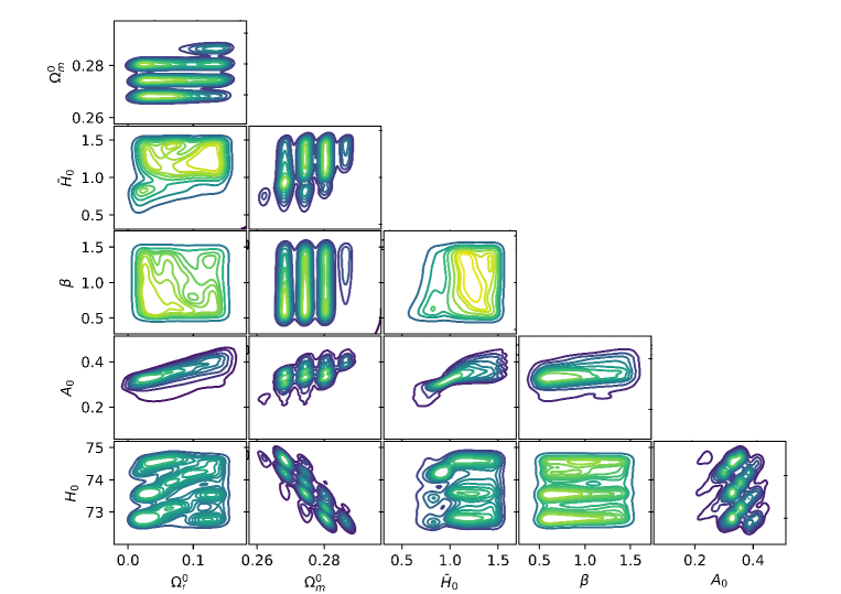
Figure 1: Density plot for all the model’s parameters. The yellow region indicates the most frequent values preferred by the model.

The obtained models are then filtered requiring non-tachyonic modes, i.e. that Eq.(9) is guaranteed, and we further impose the condition that the normalized (by $H_{0}^{2}$) squared mass is less or equal to unity, today. This point is relevant in order for the considered $f(R)$ model to obey the so-called “chameleon”  mechanism Brax:2008hh . The resulting models are thus physically viable and, to study the efficiency to alleviate the tension, we also require that $0.999<H/H_{Pl}|_{x=2.4}<1.001$ which means at $z\simeq 10$. With this procedure, we finally obtain around $5\times 10^{3}$ sampled models. We then convolve the data with a normal distribution to create a smooth density estimate. A kernel density estimate plot is a visualization method used to depict the distribution of observations in a dataset, akin to a histogram. The results are depicted in Fig.1.

From this analysis, preferred regions can be individualized providing the most frequent parameter sets. As an example of the model’s capability in alleviating the Hubble tension, we select

$$H_{0}=72.9\,,\quad\Omega_{m}^{0}=0.28\,,\quad\Omega_{r}^{0}=0.035\,,\quad\bar{H}_{0}=1.01\,,\quad A_{0}=0.33\,,\quad\beta=0.7\,.$$ (26)

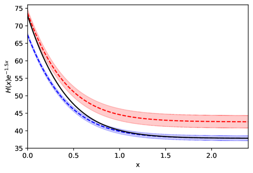
Figure 2: Plot of $H(x)$ (black) using the parameters in Eq.(26) and the profiles (with the corresponding errors) of $H_{Pl}(x)$ (blue) and $H_{SN}(x)$ (red).

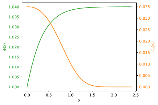
Figure 3: Plot of $\phi(x)$ (green) and $\Omega_{r}(x)$ (orange) integrated from Eqs.(20) and (21) implementing the parameters in Eq.(26).

In Fig.2, we plot the resulting evolution of $H(x)$ from Eq.(14), with this parameter setup, together with the curves in Eq.(22) (blue) and Eq.(23) (red) considering the corresponding errors. The tension alleviation emerges clearly, and the $H(x)$ profile overlaps $H_{Pl}(x)$ already at $x\simeq 1.5$, but reaches higher values of the Hubble constant in $x=0$. In Fig.3, we instead plot the functions $\phi$ and $\Omega_{r}$ as functions of $x$. The curves are obtained by integrating Eq.(20) and Eq.(21) assuming the choice of the parameters as in Eq.(26). As expected, for $x>1.5$, $\Omega_{r}(x)$ approaches zero while $\phi(x)$ frozen into a plateau.

This study of the parameter space is essential for guiding the real data analysis procedure, clearly indicating the model’s viability for interpreting the Hubble tension through the missing physics that must be added to the $\Lambda$CDM formulation to reconcile it with observations. The numerical study highlights how the additional components of modified metric $f(R)$ gravity and the radiation term generated by the cosmological background are crucial for mitigating the Hubble tension within the framework of a physical theory. In this context, a key aspect of the numerical filtering procedure is ensuring that the modified gravity is not associated with a tachyonic mode.

VI Conclusions

We constructed a revised dynamical model for the late Universe based on both a metric $f(R)$ gravity in the Jordan frame, similar to the approach in deangelis-fr-mnras , and a phenomenological model for matter creation associated with the time variation of the cosmological gravitational field. The matter creation is described by treating the Universe as an open thermodynamic system, with the rate of particle creation phenomenologically regulated by a power-law of the Hubble parameter. The form of the $f(R)$ gravity is not assigned a priori. Indeed, by imposing suitable conditions on the generalized Friedmann equation, the potential of the non-minimally coupled scalar field $V(x)\equiv V(\phi(x))$ becomes a dynamical variable, along with $\phi(x)$ and $\Omega_{r}(x)$. Consequently, it is possible to reconstruct the form of $V(\phi)$ and thus determine the function $f(R)$ governing the modified gravity.

We developed a dynamical model with six free parameters: $\{H_{0},\,\Omega_{m}^{0},\,\Omega_{r}^{0},\,\bar{H}_{0},\,A_{0},\,\beta\}$, aimed at alleviating the Hubble tension. The numerical treatment is based on a detailed screening of all the possible solutions, retaining only those parameter sets that verified the physical consistency of the proposed scenario, together with the possibility that the resulting Hubble parameter has the required asymptotic $\Lambda$CDM behavior (de facto reached already at low $z$ value) and, at the same time, allows for a Hubble constant compatible with the SH0ES Collaboration observation. The determination of a privileged set of parameters gave a significant perspective on what comparison with real data could imply on the parameter space. The resulting picture is a successful approach to the Hubble tension alleviation since the Hubble parameter quickly approaches the $\Lambda$CDM model with the Planck measured parameters, as the redshift increases.

We conclude by emphasizing that the privileged values of $\Omega_{r}^{0}$ resulted to be very small, making this component reliably unobserved through direct measurement. The particles forming this radiation component are very weakly interacting, such as sterile neutrinos 2017PhR…711….1A , which explain their elusive nature. The key takeaway from this study is that the Hubble tension can be effectively addressed by combining metric $f(R)$ gravity with additional modifications to the standard $\Lambda$CDM model.

References

- (1) Dan M. Scolnic, Dillon Brout, Anthony Carr, Adam G. Riess, Tamara M. Davis, Arianna Dwomoh, David O. Jones, Noor Ali, Pranav Charvu, Rebecca Chen, Erik R. Peterson, Brodie Popovic, Benjamin M. Rose, Charlotte M. Wood, Peter J. Brown, Ken Chambers, David A. Coulter, Kyle G. Dettman, Georgios Dimitriadis, Alexei V. Filippenko, Ryan J. Foley, Saurabh W. Jha, Charles D. Kilpatrick, Robert P. Kirshner, Yen-Chen Pan, Armin Rest, Cesar Rojas-Bravo, Matthew R. Siebert, Benjamin E. Stahl and WeiKang Zheng, ApJ 938, 113 (2022).
- (2) D. M. Scolnic, D. O. Jones, A. Rest, Y. C. Pan, R. Chornock, R. J. Foley, M. E. Huber, R. Kessler, G. Narayan, A. G. Riess, S. Rodney, E. Berger, D. J. Brout, P. J. Challis, M. Drout, D. Finkbeiner, R. Lunnan, R. P. Kirshner, N. E. Sanders, E. Schlafly, S. Smartt, C. W. Stubbs, J. Tonry, W. M. Wood-Vasey, M. Foley, J. Hand, E. Johnson, W. S. Burgett, K. C. Chambers, P. W. Draper, K. W. Hodapp, N. Kaiser, R. P. Kudritzki, E. A. Magnier, N. Metcalfe, F. Bresolin, E. Gall, R. Kotak, M. McCrum and K. W. Smith, ApJ 859, 101 (2018).
- (3) Dillon Brout et al., ApJ 938, 110 (2022).
- (4) Adam G. Riess, Wenlong Yuan, Lucas M. Macri, Dan Scolnic, Dillon Brout, Stefano Casertano, David O. Jones, Yukei Murakami, Gagandeep S. Anand, Louise Breuval, Thomas G. Brink, Alexei V. Filippenko, Samantha Hoffmann, Saurabh W. Jha, W. D’arcy Kenworthy, John Mackenty, Benjamin E. Stahl and WeiKang Zheng, ApJ Lett. 934, L7 (2022).
- (5) N. Aghanim et al., A& A 641, A6 (2020), [Erratum: Astron.Astrophys. 652, C4 (2021)].
- (6) Tiziano Schiavone, Giovanni Montani and Flavio Bombacigno, Mon. Not. RAS 522, L72 (2023).
- (7) Giovanni Montani, Mariaveronica De Angelis, Flavio Bombacigno and Nakia Carlevaro, Mon. Not. RAS 527, L156–L161 (2024).
- (8) Giovanni Montani, Nakia Carlevaro and Maria Giovanna Dainotti, Phys. Dark Univ. 44, 101486 (2024).
- (9) S.A. Adil, Ö. Akarsu, E. Di Valentino, R.C. Nunes, E. Özülker, A.A. Sen and E. Specogna, Phys. Rev. D 109, 023527 (2024).
- (10) S. Nojiri, S. D. Odintsov and V. K. Oikonomou, Nucl. Phys. B 980, 115850 (2022).
- (11) Sergei D. Odintsov, Diego Sáez-Chillón Gómez and German S. Sharov, Nucl. Phys. B 966, 115377 (2021).
- (12) B. Wang, E. Abdalla, F. Atrio-Barandela and D. Pavón, Rep. Prog. Phys. 79, 096901 (2016).
- (13) Krishna Naidoo, Mariana Jaber, Wojciech A. Hellwing and Maciej Bilicki, Phys. Rev. D 109, 083511 (2024).
- (14) Maria Giovanna Dainotti, Biagio De Simone, Tiziano Schiavone, Giovanni Montani, Enrico Rinaldi and Gaetano Lambiase, ApJ 912, 150 (2021).
- (15) Maria Giovanna Dainotti, Biagio De Simone, Tiziano Schiavone, Giovanni Montani, Enrico Rinaldi, Gaetano Lambiase, Malgorzata Bogdan and Sahil Ugale, Galaxies 10 (2022).
- (16) Bing Xu, Jiancheng Xu, Kaituo Zhang, Xiangyun Fu and Qihong Huang, Mon. Not. RAS 530, 5091 (2024).
- (17) C. Krishnan, E. Ó. Colgáin, M. M. Sheikh-Jabbari and Tao Yang, Phys. Rev. D 103, 103509 (2021).
- (18) L. Kazantzidis and L. Perivolaropoulos, Phys. Rev. D 102, 023520 (2020).
- (19) George Efstathiou, Mon. Not. RAS 505, 3866 (2021).
- (20) W. Giarè, Phys. Rev. D 123545 (2024).
- (21) Sunny Vagnozzi, Universe 9, 393 (2023).
- (22) Sunny Vagnozzi, Phys. Rev. D 102, 023518 (2020).
- (23) Thomas P. Sotiriou and Valerio Faraoni, Rev. Mod. Phys. 82, 451 (2010).
- (24) Shin’ichi Nojiri and Sergei D. Odintsov, Physics Reports 505, 59 (2011).
- (25) Giovanni Montani, Classical and Quantum Gravity 18, 193 (2001).
- (26) M. O. Calvão, J. A. S. Lima and I. Waga, Physics Letters A 162, 223 (1992).
- (27) Recai Erdem, arXiv e-prints arXiv:2402.16791 (2024).
- (28) George Efstathiou and Steven Gratton, Mon. Not. RAS 496, L91 (2020).
- (29) Gonzalo J. Olmo, Phys. Rev. D 72, 083505 (2005).
- (30) Philippe Brax, Carsten van de Bruck, Anne-Christine Davis and Douglas J. Shaw, Phys. Rev. D 78, 104021 (2008).
- (31) Kevork N. Abazajian, Phys. Rept. 711, 1 (2017).