Influence of different mutual friction models on two-way coupled quantized vortices and normal fluid in superfluid ⁴He

Abstract

We study the influence of two mutual friction models on quantized vortices and normal fluid using two-way coupled simulations of superfluid ⁴He. The normal fluid is affected by quantized vortices via mutual friction. A previous study [Y. Tang, et al. Nat. Commun. 14, 2941 (2023)] compared the time evolutions of the vortex ring radius and determined that the self-consistent two-way coupled mutual friction (S2W) model yielded better agreement with the experimental results than the two-way coupled mutual friction (2W) model whose model parameters were determined through experiments with rotating superfluid helium. In this study, we compare the two models in more detail in terms of the quantized vortex ring propagation, reconnection, and thermal counterflow. We found that the S2W model exhibits better results than the 2W model on the microscopic scale near a quantized vortex, such as during quantized vortex ring propagation and reconnection, although the S2W model requires a higher spatial resolution. For complex flows such as a thermal counterflow, the 2W model can be applied even to a low-resolution flow while maintaining the anisotropic normal fluid velocity fluctuations. In contrast, the 2W model predicts lower normal fluid velocity fluctuations than the S2W model. The two models show probability density functions with $-3$ power-law tails for the normal fluid velocity fluctuations.

I Introduction

At temperatures below 2.17 K, superfluid ⁴He is composed of an inviscid superfluid component and a viscous normal fluid component. This is known as the two-fluid model [1, 2]. The circulation of the superfluid component is quantized and behaves as a quantized vortex line with a diameter of approximately 10^-8 cm. In the hydrodynamics of superfluid ⁴He, the most extensively studied experimental phenomenon is the thermal counterflow [3, 4]. In these experiments, two baths are filled with superfluid ⁴He and connected via a channel. When one bath is heated, the normal fluid moves into the other bath through the channel. However, the superfluid moves in the opposite direction through the channel to satisfy the conservation of mass. As the heat flux increases, the relative velocity between the superfluid and normal fluid will also increases. When the relative velocity exceeds a critical value, the quantized vortices become tangled [5]. This phenomenon is known as quantum turbulence (QT).

A quantized vortex interacts with a normal fluid through mutual friction in superfluid ⁴He [6, 7, 8, 9]. A model of mutual friction [10, 11, 12] was proposed based on experimental data for uniformly rotating superfluid helium [13, 14]. This model has been used for one-way coupled simulations, where the velocity profile of the normal fluid is prescribed, and quantized vortices in QT are affected via the mutual friction between the superfluid and normal fluid [15]. Numerical simulations using the vortex filament model (VFM) with the full Biot-Savart law showed good agreement with the experimental results [16, 17, 18, 19].

The mutual friction model has also been used in two-way coupled simulations, where the normal fluid is locally affected by the quantized vortices via mutual friction. The mutual friction model used in these two-way coupled simulations is referred to as the 2W model in this study. The 2W model has been used in two-way coupled simulations with solid boundaries [20, 21], producing the anomalous anisotropic velocity fluctuations of the normal fluid in counterflow experiments [22]. However, the undisturbed velocity away from the core of the quantized vortex is assumed to be the normal fluid velocity in the 2W model [11].

Two-way coupled simulations using mutual friction with a locally disturbed normal fluid velocity have also been conducted [23, 24, 25]. The concept of a self-consistent model [26] was proposed and applied to simple configurations such as a quantized vortex ring [23] and a straight quantized vortex [27]. The recent self-consistent model [28] was updated slightly to the present self-consistent two-way coupled mutual friction model [29], which is referred to as the S2W model in this study. The S2W model adopts the theoretical friction force through a vortex line; consequently, no experimentally determined empirical parameters are required.

The time evolution of a single vortex ring radius obtained using the 2W and S2W models was compared with the experimental results, and the S2W model showed better agreement with the experimental results than the 2W model [30]. However, it is necessary to compare the performance of the two models for flows such as a vortex ring propagation, reconnection, and thermal counterflow.

Furthermore, monitoring the motion of solid hydrogen tracers in decaying QT has shown that the probability density function (PDF) of the superfluid velocity, $v$, is non-Gaussian with $1/v^{3}$ power-law tails owing to the motion of the quantized vortex [31]. These tails were reproduced in the PDF of the superfluid velocity obtained with a one-way coupled simulation of the VFM [32] and the Gross-Pitaevskii equation in a turbulent atomic Bose-Einstein condensate [33]. It would be interesting to observe the influence of the superfluid velocity on the PDF of the normal fluid using two-way coupled simulations with the two models.

In this study, two-way coupled simulations are conducted to examine the influence of the 2W and S2W models on the velocity fluctuations of a normal fluid. The remainder of this paper is organized as follows: In Section II, the basic equations, mutual friction models, and numerical conditions are described. In Section III, we present and discuss the numerical results for the vortex ring propagation, reconnection, and thermal counterflow. Finally, our conclusions are presented in Section IV.

II Basic equations and numerical conditions

II.1 Basic equations

For the superfluid, the VFM [11, 12, 15] is used to describe the equation of motion of the quantized vortices. Figure 1 (a) presents a schematic of a vortex filament. The tangential vector $\bm{s}^{\prime}$ is defined as a unit vector along the vortex line at point $\bm{s}$. The equation of motion for point $\bm{s}$ is as follows:

$$\frac{d\bm{s}}{dt}=\bm{v}_{s}+\alpha s^{\prime}\times\bm{v}_{ns}-\alpha^{\prime}\bm{s}^{\prime}\times(\bm{s}^{\prime}\times\bm{v}_{ns}),$$ (1)

where $\bm{v}_{s}$ denotes the superfluid velocity, $\bm{v}_{ns}=\bm{v}_{n}-\bm{v}_{s}$, $\bm{v}_{n}$ is the normal fluid velocity, and $\alpha$ and $\alpha$’ are the coefficients of mutual friction at a finite temperature for the 2W model [14, 11, 12].

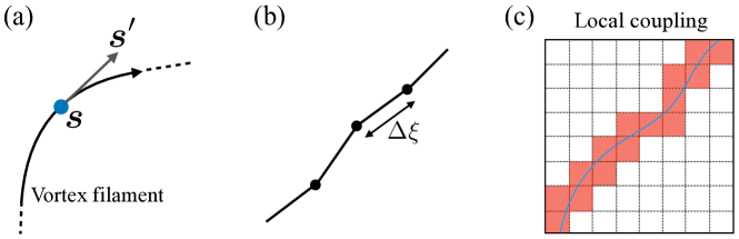
Figure 1: Schematic of a quantized vortex: (a) vortex filament and tangential vector $\bm{s}^{\prime}$ at point $\bm{s}$, (b) separated segments with $\Delta\xi$, and (c) local coupling of a quantized vortex with the normal fluid discretized on grids. The quantized vortex is coupled with the normal fluid via mutual friction in the red mesh through which the quantized vortex passes.

The superfluid velocity at 0 K at position $\bm{r}$ is obtained from the induced velocity produced from segment $d\bm{s}_{1}$ at position $\bm{s}_{1}$ using the Biot-Savart law as follows:

$$\bm{v}_{s}(\bm{r})=\frac{\kappa}{4\pi}\int_{\mathcal{L}}\frac{(\bm{s}_{1}-\bm{r})\times d\bm{s}_{1}}{|\bm{s}_{1}-\bm{r}|^{3}}+\bm{v}_{s,b}+\bm{v}_{s,a},$$ (2)

where $\kappa$ denotes the quantum circulation, $\mathcal{L}$ represents the integration along the vortex line, and $\bm{v}_{s,b}$ and $\bm{v}_{s,a}$ are the velocity induced from the boundaries and the uniform flow applied to the superfluid, respectively.

The momentum equations for the normal fluid are described by the Navier-Stokes equations:

$$\frac{\partial\bm{v}_{n}}{\partial t}+(\bm{v}_{n}\cdot\nabla)\bm{v}_{n}=-\frac{1}{\rho_{n}}\nabla P+\nu_{n}\nabla^{2}\bm{v}_{n}+\frac{1}{\rho_{n}}\bm{F}_{ns},$$ (3)

where the total density $\rho$ is composed of the superfluid density $\rho_{s}$ and normal fluid density $\rho_{n}$ as $\rho=\rho_{s}+\rho_{n}$; $P$ is the effective pressure, $\nu_{n}$ is the kinematic viscosity of the normal fluid, and $\bm{F}_{ns}$ denotes the mutual friction from the superfluid to the normal fluid. As shown in Fig. 1 (b), the mutual friction is calculated from each segment $\Delta\xi$ along the integral path $\mathcal{L^{\prime}}$ in the normal fluid mesh $\Omega^{\prime}(\bm{r})$ shown in Fig. 1 (c) at position $\bm{r}$ as follows:

$$\bm{F}_{ns}=\frac{1}{\Omega^{\prime}(\bm{r})}\int_{\mathcal{L^{\prime}}(\bm{r})}\bm{f}(\xi)d\xi,$$ (4)

where $\bm{f}(\xi)$ is the local mutual friction with arc length $\xi$.

II.2 2W model

In this study, we compare two models of mutual friction: the 2W model [11, 12] and the S2W model [29].

First, the 2W model [11, 12] is presented. The mutual friction from the superfluid to the normal fluid $\bm{f}_{sn}$ is described based on experimental results [13, 14] as follows:

$$\bm{f}_{sn}=-\alpha\rho_{s}\kappa\bm{s}^{\prime}\times\left(\bm{s}^{\prime}\times\bm{v}_{ns}\right)-\alpha^{\prime}\rho_{s}\kappa\bm{s}^{\prime}\times\bm{v}_{ns}.$$ (5)

From $\bm{f}(\xi)=\bm{f}_{ns}=-\bm{f}_{sn}$, the local mutual friction in Eq. (4) can be obtained.

$$\bm{f}(\xi)=\rho_{s}\kappa\left[\alpha\bm{s}^{\prime}\times(\bm{s}^{\prime}\times\bm{v}_{ns})+\alpha^{\prime}\bm{s}^{\prime}\times\bm{v}_{ns}\right].$$ (6)

The mutual friction $\bm{f}_{sn}$ can be interpreted from another perspective. The vortex filament is affected by the Magnus force, $\bm{f}_{M}$.

$$\bm{f}_{M}=\rho_{s}\kappa\bm{s}^{\prime}\times(\dot{\bm{s}}-\bm{v}_{s}),$$ (7)

where $\dot{\bm{s}}=d\bm{s}/dt$. In the 2W model, the drag force $\bm{f}_{D}$ is modeled using the drag coefficients $\gamma_{0}$ and $\gamma_{0}^{\prime}$ [14].

$$\bm{f}_{D}=-\gamma_{0}\bm{s}^{\prime}\times\left[\bm{s}^{\prime}\times(\bm{v}_{n}-\dot{\bm{s}})\right]+\gamma_{0}^{\prime}\bm{s}^{\prime}\times(\bm{v}_{n}-\dot{\bm{s}}).$$ (8)

Note that $\gamma_{0}$ and $\gamma_{0}^{\prime}$ correspond to $D$ and $D^{\prime}$, respectively, in reference [11]. In the 2W model, $\bm{f}_{sn}$ satisfies $\bm{f}_{sn}=\bm{f}_{D}$. Because the inertia of the quantized vortex is negligible, the equation of motion can be expressed as follows:

$$\bm{f}_{M}+\bm{f}_{D}=\bm{0}.$$ (9)

By eliminating $\dot{\bm{s}}$ using Eq. (1), we obtain the following mutual friction coefficients:

$$\alpha=\frac{\rho_{s}\kappa\gamma_{0}}{\gamma_{0}^{2}+(\rho_{s}\kappa-\gamma_{0}^{\prime})^{2}},\quad\alpha^{\prime}=\frac{\gamma_{0}^{2}-(\rho_{s}\kappa-\gamma_{0}^{\prime})\gamma_{0}^{\prime}}{\gamma_{0}^{2}+(\rho_{s}\kappa-\gamma_{0}^{\prime})^{2}}.$$ (10)

II.3 S2W model

This section discusses the S2W model [29].

In this model, the drag force is modeled using the drag coefficient $D$ as follows:

$$\bm{f}_{D}=-D\bm{s}^{\prime}\times\left[\bm{s}^{\prime}\times(\bm{v}_{n}-\dot{\bm{s}})\right].$$ (11)

When the Reynolds number Re_vortex of the normal fluid based on the velocity induced by the vortex line is low ($10^{-5}\sim 10^{-4}$), the coefficient of the drag force from the vortex line is analytically determined as follows [34]:

$$D=\frac{4\pi\rho_{n}\nu_{n}}{\frac{1}{2}-\gamma-\ln\left(\mathrm{Re}_{vortex}\right)},$$ (12)

$$\mathrm{Re}_{vortex}=\frac{|\bm{v}_{n\perp}-\dot{\bm{s}}|a_{0}}{4\nu_{n}},$$ (13)

where the subscript $\perp$ denotes a component perpendicular to the vortex line, $\gamma=0.5772$ is the Euler-Mascheroni constant, and $a_{0}$ represents the vortex core size. In this study, we set $a_{0}$ to $1.3\times 10^{-10}$ m.

In this model, the Iordanskii force [35, 36] is taken into account:

$$\bm{f}_{I}=-\rho_{n}\kappa\bm{s}^{\prime}\times(\bm{v}_{n}-\dot{\bm{s}}).$$ (14)

The equation of motion results in the following:

$$\bm{f}_{M}+\bm{f}_{D}+\bm{f}_{I}=\bm{0}.$$ (15)

The mutual friction in this model is $\bm{f}_{sn}=\bm{f}_{D}+\bm{f}_{I}$. Based on a comparison with Eq. (5), $\bm{f}_{sn}$ is modeled as follows:

$$\bm{f}_{sn}=\bm{f}_{D}+\bm{f}_{I}=-\beta\rho_{s}\kappa\bm{s}^{\prime}\times\left(\bm{s}^{\prime}\times\bm{v}_{ns}\right)-\beta^{\prime}\rho_{s}\kappa\bm{s}^{\prime}\times\bm{v}_{ns},$$ (16)

where $\beta$ and $\beta^{\prime}$ denote the coefficients of mutual friction in the S2W model. Note that to ensure $\beta^{\prime}$ is positive, the sign of $\beta^{\prime}$ is opposite that in reference [29, 39]. The definition of $\beta^{\prime}$ is consistent with $\alpha^{\prime}$ in Eq. (1) in the 2W model. Comparing the two mutual friction models in Eq. (8) and Eqs. (11) and (14), $\gamma_{0}$ and $\gamma_{0}^{\prime}$ correspond to $D$ and $-\rho_{n}\kappa$, respectively. Substituting these into Eq. (10), the following mutual friction coefficients are obtained:

$$\beta=\frac{\rho_{s}\kappa D}{D^{2}+(\rho_{s}\kappa+\rho_{n}\kappa)^{2}},\quad\beta^{\prime}=\frac{D^{2}+(\rho_{s}\kappa+\rho_{n}\kappa)\rho_{n}\kappa}{D^{2}+(\rho_{s}\kappa+\rho_{n}\kappa)^{2}}.$$ (17)

Finally, we obtain the equation of motion for $\bm{s}$ in the S2W model, similar to Eq. (1):

$$\dot{\bm{s}}=\bm{v}_{s\perp}+\beta\bm{s}^{\prime}\times\bm{v}_{ns}-\beta^{\prime}\bm{s}^{\prime}\times\left(\bm{s}^{\prime}\times\bm{v}_{ns}\right).$$ (18)

A summary and comparison of the 2W and S2W models is presented in the Appendix.

Figure 2 compares the coefficients of the 2W and S2W models as a function of the temperature, $T$. The total coefficient of the S2W model is larger than that of the 2W model, and the ratio is stable at approximately two for temperatures higher than 1.6 K, as shown in Fig. 2 (a) and (b). The fractions of $\alpha$, $\beta$, $\alpha^{\prime}$, and $\beta^{\prime}$, i.e., $\alpha/\sqrt{\alpha^{2}+\alpha^{\prime 2}}$, $\beta/\sqrt{\beta^{2}+\beta^{\prime 2}}$, $\alpha^{\prime}/\sqrt{\alpha^{2}+\alpha^{\prime 2}}$, and $\beta^{\prime}/\sqrt{\beta^{2}+\beta^{\prime 2}}$, respectively, are shown in Fig. 2 (c) and (d). $\alpha$ is dominant at all temperatures in the 2W model, whereas $\beta$ decreases gradually with increasing temperature. In contrast, $\beta^{\prime}$ increases with increasing temperature. These differences affect the strength of the mutual friction around the quantized vortex, as discussed in Section III.

Figure 2: Comparison of the coefficients of the 2W and S2W models as a function of temperature, $T$: (a) total coefficient, (b) coefficient ratio, (c) coefficient fraction of $\alpha$ and $\beta$, and (d) coefficient fraction of $\alpha^{\prime}$ and $\beta^{\prime}$. Note that coefficient fraction (c) $+$ coefficient fraction (d) $\neq 1$.

II.4 Numerical methods and conditions

Figure 3: Time evolution of the radius of a quantized vortex ring in the S2W model for 1.7 K (black), 1.8 K (red) and 2.0 K (green); open symbols: reference results [39].

Time integration of Eqs. (1) or (18) is performed using the fourth-order accuracy Runge-Kutta method with $\Delta t=$ 0.0001 s. The spatial resolution of $\xi$ between discrete points is set to 0.0008 cm $<\Delta\xi<$ 0.0024 cm. Two filaments are considered to be reconnected if they approach within $\xi_{min}=$ 0.0008 cm [16]. Short filaments of less than $5\Delta\xi_{min}$ are removed [37].

Equations (3) for the normal fluid are discretized using the second-order accuracy finite difference method. The simplified Maker and Cell method [38] is used to couple the velocity and pressure, and the fast Fourier transform is used to solve the Poisson equation for the pressure.

A temperature, $T$, of 1.9 K is considered. A box size of $D_{x}=D_{y}=D_{z}=$ 1 mm is used, and the number of grid points for the normal fluid is set to $N_{x}=N_{y}=N_{z}=120$.

Periodic conditions are adopted, and the uniform flow $\bm{v}_{s,a}=-\rho_{n}\bm{V}_{n}/\rho_{s}$ based on the mass conservation law is applied to the thermal counterflow, where $V_{n}$ is the mean velocity of the normal fluid. In this study, $V_{n}$ of 2.5 mm/s and 5.0 mm/s in the $x$ direction are considered.

For the quantized vortex ring propagation, the initial radius is set to 0.02 cm. For the reconnection, two quantized vortices cross at a 90-degree angle, and the initial distance is set to 0.002 cm.

Our implementation of the S2W model is then validated. Figure 3 shows the time evolution of the radius of a quantized vortex ring using the S2W model for 1.7, 1.8, and 2.0 K. The initial radius is set to $7.6\times 10^{-3}$ cm. The results show good agreement with the data presented in Ref. [39].

III Numerical results and discussion

III.1 Quantized vortex ring propagation

Figure 4 shows the quantized vortex ring propagation at 0.05 s for the 2W and S2W models; the quantized vortex is visualized in red and the normal fluid vortex tube is displayed in green using the second invariant of the velocity gradient tensor $Q=0.5$ $s^{-2}$ [40]. The second invariant is defined as $Q=(W_{ij}W_{ij}-S_{ij}S_{ij})/2$ using the velocity strain tensor $S_{ij}=(\partial v_{n,j}/\partial x_{i}+\partial v_{n,i}/\partial x_{j})/2$ and the vorticity tensor $W_{ij}=(\partial v_{n,j}/\partial x_{i}-\partial v_{n,i}/\partial x_{j})/2$. For the 2W model, a pair of rings of normal fluid vortex tubes are located inside and outside the quantized vortex ring in the radial direction. In the S2W model, the inner vortex tube remains slightly behind the quantized vortex ring, and the outer vortex tube propagates slightly ahead of the quantized vortex ring. This difference between the models has also been observed at 1.65 K [30]. This is due to the coefficients of mutual friction of $\alpha$ ($\alpha^{\prime}$) and $\beta$ ($\beta^{\prime}$).

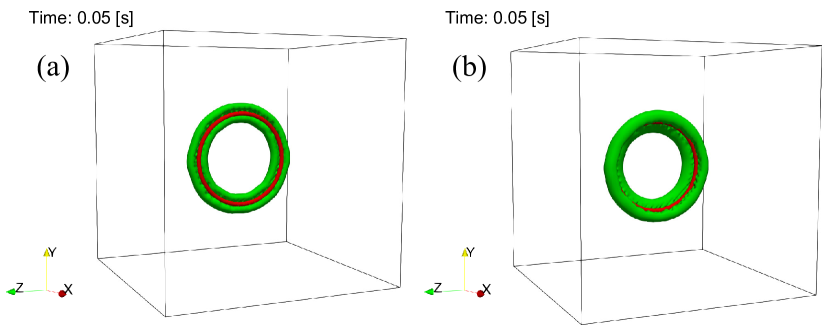
Figure 4: Quantized vortex ring propagation at 1.9 K and 0.05 s in the (a) 2W model and (b) S2W model; red color: quantized vortex, green color: normal fluid vortex tube ($Q=0.5$ $s^{-2}$).

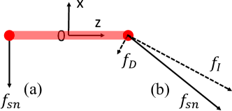
Figure 5: Mutual friction to the vortex ring $f_{sn}$ on the $x-z$ plane at 1.9 K and 0.05 s in the (a) 2W model $\bm{f}_{sn}=(-8.62\times 10^{-10},9.50\times 10^{-12})$ N/m and (b) S2W model with $\bm{f}_{D}=(-3.12\times 10^{-10},-1.69\times 10^{-10})$ N/m and $\bm{f}_{I}=(-9.25\times 10^{-10},1.71\times 10^{-9})$ N/m where $\bm{f}_{sn}=\bm{f}_{D}+\bm{f}_{I}=(-1.24\times 10^{-9},1.54\times 10^{-9})$ N/m; red color: quantized vortex; O indicates the center of the quantized vortex ring.

The mutual friction to the vortex ring $f_{sn}$ on the $x-z$ plane at 0.05 s is shown in Fig. 5. The mutual friction in the 2W model acts opposite to the propagation direction of the ring. However, the mutual friction in the S2W model acts in a diagonal direction. These orientations of the mutual friction are consistent with those shown in Fig. 2(c) and (d). As the temperature increases, the direction of the mutual friction in the S2W model rotates from $-x$ to $z$. The mutual friction in the S2W model is approximately 2.3 times stronger than that in the 2W model. This result is consistent with the coefficient ratio in Fig. 2(b). $f_{D}$ is much weaker than $f_{I}$ and acts inside the ring, whereas $f_{I}$ acts outside the ring, where $\bm{f}_{sn}=\bm{f}_{D}+\bm{f}_{I}$. Substituting Eq. (18) into Eqs. (11) and (14) results in the following:

$$\bm{f}_{D}=-D\left[(1-\beta^{\prime})\bm{s}^{\prime}\times(\bm{s}^{\prime}\times\bm{v}_{ns})+\beta\bm{s}^{\prime}\times\bm{v}_{ns}\right],$$ (19)

$$\bm{f}_{I}=\rho_{n}\kappa\left[\beta\bm{s}^{\prime}\times(\bm{s}^{\prime}\times\bm{v}_{ns})-(1-\beta^{\prime})\bm{s}^{\prime}\times\bm{v}_{ns}\right],$$ (20)

where

$$D=\frac{\rho_{s}\kappa\beta}{\beta^{2}+(1-\beta^{\prime})^{2}},$$ (21)

$$\rho_{n}\kappa=\frac{\rho_{s}\kappa\left[-\beta^{2}+\beta^{\prime}(1-\beta^{\prime})\right]}{\beta^{2}+(1-\beta^{\prime})^{2}}.$$ (22)

It is worth noting that the mutual friction predicted by the S2W model should approach that predicted by the 2W model at the coarse-graining limit. If experiments are performed to investigate the location of normal fluid vortex tubes around a vortex ring, the accuracy of the S2W model will be improved.

The time evolution of the kinetic energy per unit density of the normal fluid and superfluid is shown in Fig. 6. The kinetic energies of the normal fluid and superfluid are defined as follows:

$$\frac{E_{n}}{\rho_{n}}=\frac{1}{2}v_{n}^{2},\quad\frac{E_{s}}{\rho_{s}}=\frac{1}{2}v_{s}^{2}$$ (23)

The energy of the superfluid is gradually decreased by transferring energy to the normal fluid via mutual friction. The superfluid vortex ring in the 2W model disappears at 1.0 s, whereas that in the S2W model annihilates at 0.9 s. The superfluid energy in the 2W model maintains a longer lifetime than that in the S2W model. This result is consistent with that at 1.65 K [30]. The normal fluid energy in the S2W model increases faster than that in the 2W model. After annihilation of the superfluid vortex ring, the normal fluid energy decreases owing to the viscosity of the normal fluid.

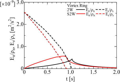
Figure 6: Time evolution of the kinetic energy per unit density of the normal fluid (solid line) and superfluid (dashed line) at 1.9 K during vortex ring propagation; black color: 2W model, red color: S2W model.

Next, the PDFs are compared. Figure 7 shows the PDFs of the velocity fluctuations during the vortex ring propagation. Superfluid velocity fluctuations are known to have strong non-Gaussian PDFs with $-3$ power-law tails [31], as shown in Fig. 7 (c) and (d). The superfluid PDFs shown with solid lines correspond to the event immediately before annihilation of the quantized vortex rings. No dashed lines are shown because the quantized vortex ring disappears.

Normal fluid velocity fluctuations are known to have Gaussian PDFs, although those velocity gradients yield non-Gaussian PDFs [43, 44, 45]. The PDFs of the normal fluid velocity fluctuations in the $y$ (radial) direction have $-3$ power-law tails, as shown by the fine solid line. The PDFs are affected by the superfluid fluctuations via mutual friction. The dashed lines indicate the normal fluid PDFs immediately after the annihilation of the quantized vortex rings. The PDFs with strong fluctuations are reduced because the superfluid vortex rings disappear. Figure 7 (a) presents the normal fluid PDFs in the $x$ (propagation) direction. The PDFs have $-3$ power-law tails, which are affected by the superfluid fluctuations via mutual friction. However, the tails exist only in the propagation direction, i.e., in the positive $x$ direction. The peaks of the PDFs are located at approximately $-0.5$. This is due to the normal fluid backflow in the inner region of the quantized vortex ring. As shown in Fig. 4, the inner normal fluid vortex caused by the quantized vortex ring rotates through mutual friction and produces the backflow in the inside of the vortex ring. The backflow is rectified by the normal fluid contraction flows induced by mutual friction. Consequently, it is believed that almost no negative fluctuations occur. In terms of the PDFs, almost no difference between the models is observed.

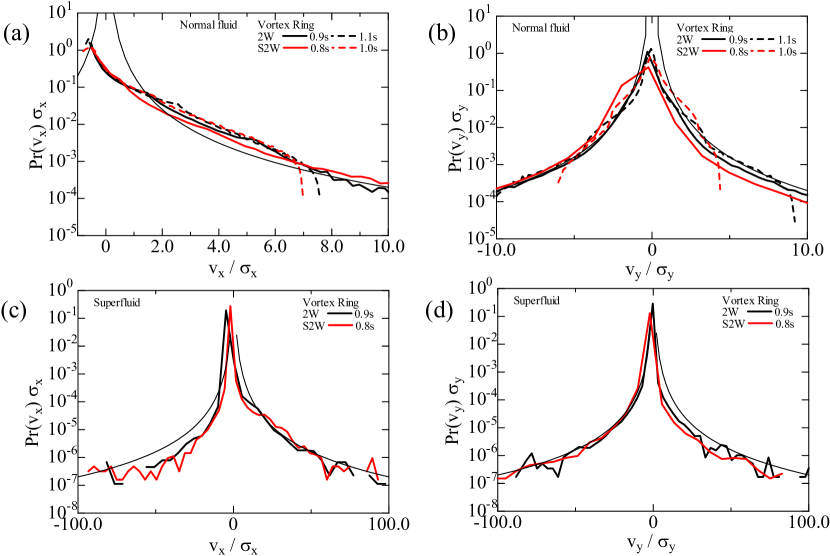
Figure 7: PDFs of velocity fluctuations at 1.9 K during vortex ring propagation for the normal fluid in the (a) $x$ (propagation) and (b) $y$ (radial) directions and the superfluid in the (c) $x$ and (d) $y$ directions; black color: 2W model at 0.9 s (solid line) and 1.1 s (dashed line), red color: S2W model at 0.8 s (solid line) and 1.0 s (dashed line); solid line: immediately before annihilation, dashed line: immediately after annihilation; fine solid line: $1/v^{3}$.

III.2 Reconnection of two quantized vortices

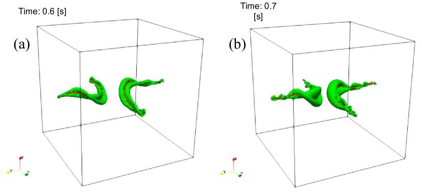
Figure 8: Vortex tubes and quantized vortices after reconnection in the (a) 2W model and (b) S2W model; red color: quantized vortex, green color: normal fluid vortex tube ($Q=0.5$ $s^{-2}$).

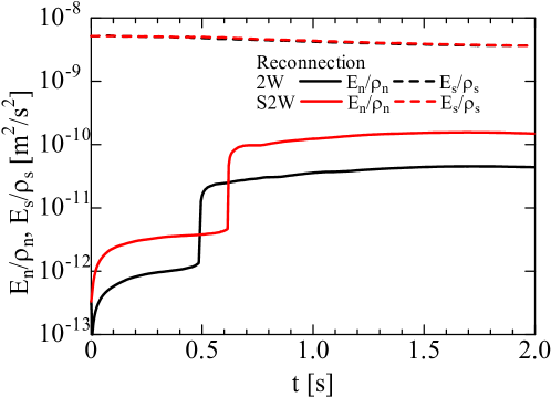
Figure 9: Time evolution of the kinetic energy per unit density of the normal fluid (solid line) and superfluid (dashed line) during reconnection; black color: 2W model, red color: S2W model.

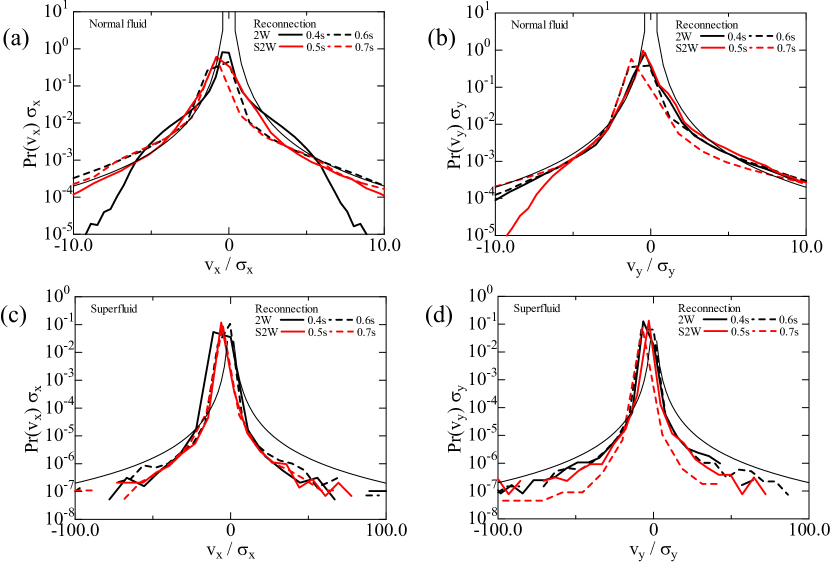
Figure 10: PDFs of the velocity fluctuations during reconnection for the normal fluid in the (a) $x$ (quantized vortex propagation) and (b) $y$ (perpendicular) directions and the superfluid in the (c) $x$ and (d) $y$ directions; black color: 2W model at 0.4 s (solid line) and 0.6 s (dashed line), red color: S2W model at 0.5 s (solid line) and 0.7 s (dashed line); solid line: immediately before reconnection, dashed line: immediately after reconnection; fine solid line: $1/v^{3}$.

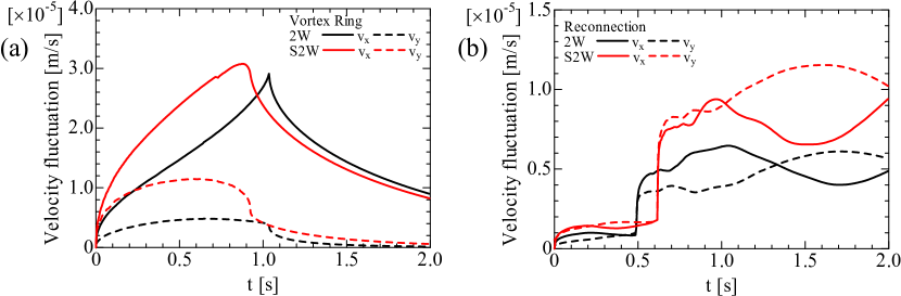
Figure 11: Velocity fluctuations of the normal fluid in the x (solid line) and y (dashed line) directions during (a) vortex ring propagation and (b) reconnection; black color: 2W model, red color: S2W model.

The vortex tubes and quantized vortices after reconnection are shown in Fig. 8; the quantized vortex is shown in red, and the normal fluid vortex tube is depicted in green using the second invariant $Q=0.5$ s^-2 of the velocity gradient tensor. For the S2W model, the spiral vortex tubes that emerge around the quantized vortex line have a stronger twist than those in the 2W model.

Figure 9 shows the time evolution of the kinetic energy per unit density of the normal fluid and superfluid during reconnection. Before reconnection, the two quantized vortices are twisted while approaching each other owing to the induced velocity from the other quantized vortex. The motion of the quantized vortices produces a weak vortex tube of normal fluid via mutual friction. Consequently, the energy of the superfluid is transferred to the normal fluid. An abrupt energy transfer from the superfluid to the normal fluid occurs at approximately 0.5 s. Because the S2W model has stronger mutual friction than the 2W model, the reconnection is delayed. The normal fluid in the S2W model has a higher energy than that in the 2W model owing to the stronger mutual friction.

Figure 10 shows the PDFs of the velocity fluctuations during reconnection. The PDFs of the normal fluid and superfluid exhibit $-3$ power-law tails in all directions. This is due to the superfluid fluctuations. Although there is almost no difference in the superfluid PDFs between the two models, the normal fluid PDFs drawn with solid lines appear different, as shown in Fig. 10 (a) and (b). The solid lines correspond to the time immediately before reconnection. The normal fluid fluctuations remain weak, as shown in Fig. 9 because the influence of the mutual friction on the normal fluid is weak. Consequently, the PDFs do not yet exhibit $-3$ power-law long tails, i.e., the PDFs show the results during a transient process. Nevertheless, the two models produce different PDFs. This is due to the difference in the location of the normal fluid vortex tubes around the quantized vortex, as shown in Fig. 4.

Figure 11 (a) shows the velocity fluctuations of the normal fluid in the $x$ and $y$ directions during vortex ring propagation. The velocity fluctuation is defined as the root-mean-square velocity $\sqrt{v_{n,i}^{2}}$ $(i=x,y)$. The normal fluid in the S2W model receives a greater amount of energy than that in the 2W model. The velocity fluctuation in the $x$ direction is stronger than that in the $y$ direction. This is a result of jet formation of the normal fluid due to the local mutual friction $\bm{f}_{ns}=-\bm{f}_{sn}$ as shown in Fig. 5. Figure 11 (b) shows the velocity fluctuations of the normal fluid in the $x$ and $y$ directions during reconnection. As an initial condition, two straight quantized vortex lines crossed at a 90-degree angle are set at a certain distance in the $x$ (vertical) direction. Immediately after reconnection, the 2W model yields a stronger fluctuation in the $x$ direction, whereas the S2W model yields a stronger fluctuation in the $y$ direction. This is due to the location of the normal fluid vortex tubes produced around the quantized vortex line, as shown in Figs. 4 and 8.

III.3 Thermal counterflow

This section considers the thermal counterflow. Figure 12 shows a snapshot of the quantized vortices and normal fluid vortex tubes in a thermal counterflow. The vortex tubes are produced by mutual friction with quantized vortices. The S2W model yields a high density of vortex lines and strong vortex tubes. The vortex line density is defined as the vortex line length per unit volume. The time evolution of the vortex line density in the thermal counterflow is shown in Fig. 13. The density gradually increases at 2.5 mm/s, whereas it increases rapidly at 5.0 mm/s. Subsequently, the density reaches a statistically steady state. The S2W model yields a density that is approximately twice that of the 2W model. Figure 14 shows the average vortex line density in the statistically steady state of Fig. 13 as a function of the mean relative velocity, $V_{ns}$. The slope parameter $\gamma=L^{1/2}/(V_{ns}-v_{0})$ is presented in the figure, where $v_{0}$ is a small, adjustable parameter on the order of 1 cm s^-1. The value $\gamma=167$ of 2W^∗ is the reference value in our previous study using the 2W model [22] and is consistent with the present result of $\gamma=160$ obtained using the 2W model. The S2W model yields a higher $\gamma=187$ than the 2W model, although the experimental value is $\gamma\sim 130$ s/cm² [41, 42].

The Vinen equation [4, 8] can be expressed as follows:

$$\frac{dL}{dt}=A|V_{ns}|L^{3/2}-BL^{2},$$ (24)

where $A$ and $B$ denote the coefficients of the generation and decay rates, respectively. In the steady state, $L^{1/2}=A/B|V_{ns}|$ is obtained. Here, $A/B\sim\gamma$. As shown in Fig. 9, the stronger mutual friction in the S2W model leads to a slower approach between two quantized vortices. Consequently, the decay rate becomes low, and thus the S2W model estimates a larger $\gamma$ than the 2W model.

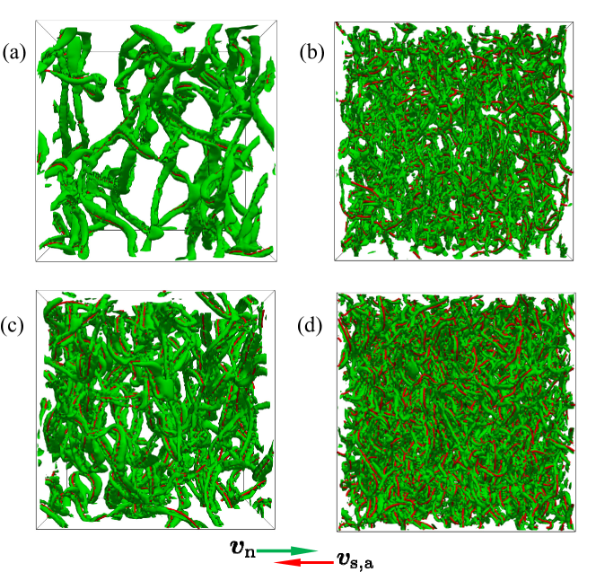
Figure 12: Quantized vorticies (red) and normal fluid vortex tubes (green) in a thermal counterflow for the 2W model (a) $v_{n}=2.5$ mm/s ($Q=10$ $s^{-2}$), (b) $v_{n}=5.0$ mm/s ($Q=100$ $s^{-2}$) and S2W model (c) $v_{n}=2.5$ mm/s ($Q=100$ $s^{-2}$), (d) $v_{n}=5.0$ mm/s ($Q=1000$ $s^{-2}$).

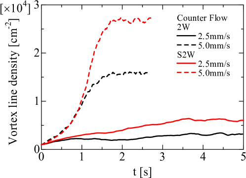
Figure 13: Time evolution of the vortex line density in the thermal counterflow for the 2W model and S2W model at $v_{n}=2.5$ and 5.0 mm/s.

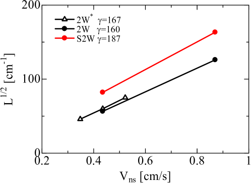
Figure 14: Average vortex line density in the statistically steady state of Fig. 13 as a function of the mean relative velocity, $V_{ns}$, where $\gamma=L^{1/2}/(V_{ns}-v_{0})$ and $v_{0}$ is a small, adjustable parameter on the order of 1 cm s^-1; 2W^∗ denotes the result in our previous study using the 2W model [22].

The PDFs of the velocity fluctuations in the thermal counterflow in the statistically steady state are shown in Fig. 15. Two mean normal fluid velocities of 2.5 mm/s and 5.0 mm/s are examined. There is no difference in the direction of fluctuations in the PDFs of the superfluid. The PDFs of the normal fluid in the $x$ and $y$ directions exhibit Gaussian distributions with weak fluctuations. As shown in Fig. 15 (b), strong fluctuations exhibit $-3$ power-law tails. The S2W model yields stronger fluctuations than the 2W model owing to the stronger mutual friction. The mean normal fluid velocity has a weak influence on the intensity of the PDFs of the normal fluid. The PDFs in the $x$ (streamwise) direction appear asymmetric in Fig. 15 (a). The positive fluctuations exhibit sub-Gaussian distributions, whereas the negative fluctuations produce $-3$ power-law tails. In this study, the normal fluid flows in the positive $x$ direction, and the superfluid moves in the negative $x$ direction during the counterflow. If quantized vortex rings are generated, they tend to propagate in the negative $x$ direction. Consequently, long-tail PDFs are produced in the propagation direction of the quantized vortex rings, as shown in Fig. 7 (a).

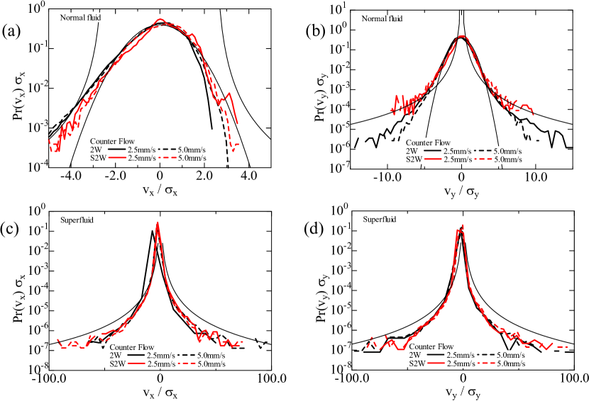
Figure 15: PDFs of velocity fluctuations in the thermal counterflow for the normal fluid in the (a) $x$ (streamwise) and (b) $y$ (perpendicular) directions and the superfluid in the (c) $x$ and (d) $y$ directions; black color: 2W model, red color: S2W model; solid line: mean normal fluid velocity of 2.5 mm/s, dashed line: 5.0 mm/s; fine solid line: $1/v^{3}$ and Gaussian profile for (a) and (b).

Figure 16 shows the normal fluid velocity fluctuations in the 2W and S2W models as a function of the mean normal fluid velocity in the thermal counterflow. At a low resolution, the 2W model reproduces the anisotropic fluctuations, whereas the S2W model produces fewer anisotropic fluctuations. At high resolution, the 2W model yields almost the same fluctuations as the low-resolution model, whereas the S2W model generates anisotropic fluctuations. The S2W model requires higher resolution and yields higher fluctuations than the 2W model. However, the S2W model predicts the normal fluid fluctuations better than the 2W model.

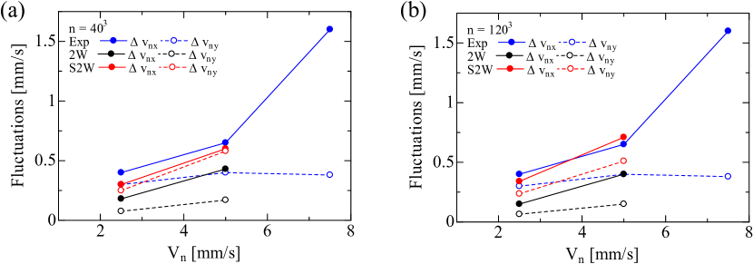
Figure 16: Normal fluid velocity fluctuations in the $x$ (streamwise, solid line) and $y$ (perpendicular, dashed line) directions as a function of the mean normal fluid velocity, $V_{n}$, in the thermal counterflow for grid numbers of (a) $40^{3}$ and (b) $120^{3}$; Exp: experimental results (blue) [46], 2W model (black), and S2W model (red).

IV Conclusions

We investigated the performance of two different mutual friction models, i.e., the 2W and S2W models, on quantized vortices and normal fluid using two-way coupled simulations of superfluid ⁴He. In the quantized vortex ring propagation and reconnection, the normal fluid vortex tube induced by mutual friction is produced at slightly different locations around the quantized vortex in each model. The normal fluid velocity fluctuations in the S2W model are stronger than those in the 2W model, whereas the probability density functions produced by the two models show negligible differences.

The S2W model is better suited for describing the normal fluid physics on a microscopic scale near a quantized vortex, such as during quantized vortex ring propagation and reconnection. For complex flows, such as a thermal counterflow, the 2W model can represent a low-resolution flow while maintaining anisotropic fluctuations. However, the S2W model requires higher resolution and yields higher fluctuations than the 2W model. The two-way coupled simulation with each model produces PDFs with $-3$ power-law tails for the normal fluid velocity fluctuations.

*

Appendix A Summary of the 2W and S2W models

We summarize and compare the parameters, forces, and equations of motion of the 2W and S2W models in Table 1.

Table 1: Comparison of the 2W model and S2W model

2W model	S2W model
$\alpha=\frac{\rho_{s}\kappa\gamma_{0}}{\gamma_{0}^{2}+(\rho_{s}\kappa-\gamma_{0}^{\prime})^{2}}$	$\beta=\frac{\rho_{s}\kappa D}{D^{2}+(\rho_{s}\kappa+\rho_{n}\kappa)^{2}}$
$\alpha^{\prime}=\frac{\gamma_{0}^{2}-(\rho_{s}\kappa-\gamma_{0}^{\prime})\gamma_{0}^{\prime}}{\gamma_{0}^{2}+(\rho_{s}\kappa-\gamma_{0}^{\prime})^{2}}$	$\beta^{\prime}=\frac{D^{2}+(\rho_{s}\kappa+\rho_{n}\kappa)\rho_{n}\kappa}{D^{2}+(\rho_{s}\kappa+\rho_{n}\kappa)^{2}}$
$\gamma_{0}=\frac{\rho_{s}\kappa\alpha}{\alpha^{2}+(1-\alpha^{\prime})^{2}}$	$D=\frac{\rho_{s}\kappa\beta}{\beta^{2}+(1-\beta^{\prime})^{2}}$
$\gamma_{0}^{\prime}=\frac{\rho_{s}\kappa\left[\alpha^{2}-\alpha^{\prime}(1-\alpha^{\prime})\right]}{\alpha^{2}+(1-\alpha^{\prime})^{2}}$	$\rho_{n}\kappa=\frac{\rho_{s}\kappa\left[-\beta^{2}+\beta^{\prime}(1-\beta)\right]}{\beta^{2}+(1-\beta^{\prime})^{2}}$
$\bm{f}_{M}=\rho_{s}\kappa\bm{s}^{\prime}\times(\dot{\bm{s}}-\bm{v}_{s})$	$\bm{f}_{M}=\rho_{s}\kappa\bm{s}^{\prime}\times(\dot{\bm{s}}-\bm{v}_{s})$
$\bm{f}_{D}=-\gamma_{0}\bm{s}^{\prime}\times\left[\bm{s}^{\prime}\times(\bm{v}_{n}-\dot{\bm{s}})\right]+\gamma_{0}^{\prime}\bm{s}^{\prime}\times(\bm{v}_{n}-\dot{\bm{s}})$	$\bm{f}_{D}=-D\bm{s}^{\prime}\times\left[\bm{s}^{\prime}\times(\bm{v}_{n}-\dot{\bm{s}})\right]$
	$\bm{f}_{I}=-\rho_{n}\kappa\bm{s}^{\prime}\times(\bm{v}_{n}-\dot{\bm{s}})$
$\bm{f}_{M}+\bm{f}_{D}=\bm{0}$	$\bm{f}_{M}+\bm{f}_{D}+\bm{f}_{I}=\bm{0}$
$\bm{f}_{sn}=\bm{f}_{D}$	$\bm{f}_{sn}=\bm{f}_{D}+\bm{f}_{I}$
$\bm{f}_{sn}=-\alpha\rho_{s}\kappa\bm{s}^{\prime}\times\left(\bm{s}^{\prime}\times\bm{v}_{ns}\right)-\alpha^{\prime}\rho_{s}\kappa\bm{s}^{\prime}\times\bm{v}_{ns}$	$\bm{f}_{sn}=-\beta\rho_{s}\kappa\bm{s}^{\prime}\times\left(\bm{s}^{\prime}\times\bm{v}_{ns}\right)-\beta^{\prime}\rho_{s}\kappa\bm{s}^{\prime}\times\bm{v}_{ns}$
$\dot{\bm{s}}=\bm{v}_{s}+\alpha s^{\prime}\times\bm{v}_{ns}-\alpha^{\prime}\bm{s}^{\prime}\times(\bm{s}^{\prime}\times\bm{v}_{ns})$	$\dot{\bm{s}}=\bm{v}_{s\perp}+\beta\bm{s}^{\prime}\times\bm{v}_{ns}-\beta^{\prime}\bm{s}^{\prime}\times\left(\bm{s}^{\prime}\times\bm{v}_{ns}\right)$

References

- [1] L. Tisza, Transport phenomena in helium II, Nature 141, 913 (1938).
- [2] L. D. Landau, The theory of superfluidity of helium II, J. Phys. USSR 5, 71 (1941), reprinted in I. M. Khalatnikov, An Introduction to the Theory of Superfluidity (Perseus Publishing, Cambridge, 2000).
- [3] C. J. Gorter and J. H. Mellink, On the irreversible processes in liquid helium II, Physica, 15, 285 (1949).
- [4] J. T. Tough, Superfluid turbulence, in P͡rog. in Low Temp. Phys., edited by D. F. Brewer (North-Holland, Amsterdam, 1982), Vol. 8, Chap. 3.
- [5] R. P. Feynman, Application of quantum mechanics to liquid helium, in Progress in Low-Temperature Physics, edited by C. J. Gorter (North-Holland, Amsterdam, 1957), Vol. I, p. 17.
- [6] W. F. Vinen, Mutual friction in a heat current in liquid helium II. I. Experiments on steady heat currents, Proc. R. Soc. Lond. A 240, 114 (1957).
- [7] W. F. Vinen, Mutual friction in a heat current in liquid helium II. II. Experiments on transient effects, Proc. R. Soc. Lond. A 240, 128 (1957).
- [8] W. F. Vinen, Mutual friction in a heat current in liquid helium II. III. Theory of the mutual friction, Proc. R. Soc. Lond. A 242, 493 (1957).
- [9] W. F. Vinen, Mutual friction in a heat current in liquid helium II. IV. Critical heat currents in wide channels, Proc. R. Soc. Lond. A 243, 400 (1958).
- [10] H. E. Hall and W. F. Vinen, The rotation of liquid helium II II. The theory of mutual friction in uniformly rotating helium II, Proc. R. Soc. Lond. A 238, 215 (1956).
- [11] K. W. Schwarz, Turbulence in superfluid helium: Steady homogeneous counterflow, Phys. Rev. B 18, 245 (1978).
- [12] K. W. Schwarz, Three-dimensional vortex dynamics in superfluid 4He: Line-line and line-boundary interactions, Phys. Rev. B 31, 5782 (1985).
- [13] H. E. Hall and W. F. Vinen, The rotation of liquid helium II I. Experiments on the propagation of second sound in uniformly rotating helium II, Proc. R. Soc. Lond. A 238, 204 (1956).
- [14] C. F. Barenghi, R. J. Donnelly, and W. F. Vinen, Friction on quantized vortices in helium II. A review, J. Low Temp. Phys. 52, 189 (1983).
- [15] K. W. Schwarz, Three-dimensional vortex dynamics in superfluid: Homogeneous superfluid turbulence, Phys. Rev. B 38, 2398 (1988).
- [16] H. Adachi, S. Fujiyama, and M. Tsubota, Steady-state counterflow quantum turbulence: Simulation of vortex filaments using the full Biot-Savart law, Physical Review B, 81 104511 (2010).
- [17] A. W. Baggaley, L. K. Sherwin, C. F. Barenghi, and Y. A. Sergeev, Thermally and mechanically driven quantum turbulence in helium II, Phys. Rev. B 86, 104501 (2012).
- [18] L. Kondaurova, V. L’vov, A. Pomyalov, and I. Procaccia, Structure of a quantum vortex tangle in 4He counterflow turbulence, Phys. Rev. B 89, 014502 (2014).
- [19] S. Yui and M. Tsubota, Counterflow quantum turbulence of He-II in a square channel: Numerical analysis with nonuniform flows of the normal fluid, Phys. Rev. B 91, 184504 (2015).
- [20] D. Khomenko, P. Mishra, and A. Pomyalov, Coupled dynamics for superfluid 4He in a channel, J. Low Temp. Phys. 187, 405 (2017).
- [21] S. Yui, M. Tsubota, and H. Kobayashi, Three-dimensional coupled dynamics of the two-fluid model in superfluid: Deformed velocity profile of normal fluid in thermal counterflow, Phys. Rev. Lett. 120, 155301 (2018).
- [22] S. Yui, H. Kobayashi, M. Tsubota, and W. Guo, Fully coupled two-fluid dynamics in superfluid 4He: Anomalous anisotropic velocity fluctuations in counterflow, Phys. Rev. Lett. 124, 155301 (2020).
- [23] D. Kivotides, C. F. Barenghi, and D. C. Samuels, Triple vortex ring structure in superfluid helium II, Science, 290, 777 (2000).
- [24] D. Kivotides, Relaxation of superfluid vortex bundles via energy transfer to the normal fluid, Phys. Rev. B 76, 054503 (2007).
- [25] D. Kivotides, Spreading of superfluid vorticity clouds in normal fluid turbulence, J. Fluid Mech. 668, 58 (2011).
- [26] O. C. Idowu, D. Kivotides, C. F. Barenghi, and D. C. Samuels, Equation for self-consistent superfluid vortex line dynamics, J. Low Temp. Phys. 120, 269 (2000).
- [27] O. C. Idowu, A. Willis, C. F. Barenghi, and D. C. Samuels, Local normal fluid helium II flow due to mutual friction interaction with the superfluid, Phys. Rev. B 62, 3409 (2000).
- [28] D. Kivotides, Superfluid helium-4 hydrodynamics with discrete topological defects, Phys. Rev. Fluids 3, 104701 (2018).
- [29] L. Galantucci, A. W. Baggaley, C. F. Barenghi, and G. Krstulovic, A new self-consistent approach of quantum turbulence in superfluid helium, Eur. Phys. J. Plus 135, 547 (2020).
- [30] Y. Tang, W. Guo, H. Kobayashi, S. Yui, M. Tsubota, and T. Kanai, Imaging quantized vortex rings in superfluid helium to evaluate quantum dissipation, Nat. Commun. 14, 2941 (2023).
- [31] M. S. Paoletti, M. E. Fisher, K. R. Sreenivasan, and D. P. Lathrop, Velocity statistics distinguish quantum turbulence from classical turbulence, Phys. Rev. Lett 101, 154501 (2008).
- [32] H. Adachi and M. Tsubota, Numerical study of velocity statistics in steady counterflow quantum turbulence, Physical Review B, 83 132503 (2011).
- [33] A. C. White, C. F. Barenghi, N. P. Proukakis, A. J. Youd, and D. H. Wacks, Nonclassical velocity statistics in a turbulent atomic Bose-Einstein condensate, Physical Review Letters, 104 075301 (2010).
- [34] S. Kaplun, Low Reynolds number flow past a circular cylinder, J. Math. Mech. 6, 595 (1957).
- [35] G. E. Volovik, Three nondissipative forces on a moving vortex line in superfluids and superconductors, JETP Lett. 62, 1 (1995).
- [36] L. Thompson and P. C. E. Stamp, Quantum dynamics of a Bose superfluid vortex, Phys. Rev. Lett. 108, 184501 (2012).
- [37] M. Tsubota, T. Araki, and S. K. Nemirovskii, Dynamics of vortex tangle without mutual friction in superfluid 4He, Phys. Rev. B 62, 11751 (2000).
- [38] F. H. Harlow and J. E. Welch, Numerical calculation of time-dependent viscous incompressible flow of fluid with free surface, Phys. Fluids 8, 2182 (1965).
- [39] L. Galantucci, G. Krstulovic, and C. F. Barenghi, Friction-enhanced lifetime of bundled quantum vortices, Phys. Rev. Fluids 8, 014702 (2023).
- [40] J. C. R. Hunt, A. A. Wray, and P. Moin, Eddies, streams, and convergence zones in turbulent flows, in Proceedings of the Summer Program 1988, Center for Turbulence Research, Stanford Univ. 88, 193 (1988).
- [41] J. T. Tough, Superfluid turbulence, in Prog. in Low Temp. Phys., edited by D. F. Brewer (North-Holland, Amsterdam, 1982), Vol. 8, Chap. 3.
- [42] R. K. Childers and J. T. Tough, Phys. Rev. B 13, 1040 (1976).
- [43] A. Noullez, G. Wallace, W. Lempert, R. B. Miles, and U. Frisch, Transverse velocity increments in turbulent flow using the RELIEF technique, J. Fluid Mech. 339, 287 (1997).
- [44] A. Vincent and M. Meneguzzi, The spatial structure and statistical properties of homogeneous turbulence, J. Fluid Mech. 225, 1 (1991).
- [45] T. Gotoh, D. Fukayama, and T. Nakano, Velocity field statistics in homogeneous steady turbulence obtained using a high-resolution direct numerical simulation, Phys. Fluids 14, 1065 (2002).
- [46] B. Mastracci, S. Bao, W. Guo, and W. F. Vinen, Particle tracking velocimetry applied to thermal counterflow in superfluid 4He: Motion of the normal fluid at small heat fluxes, Phys. Rev. Fluids 4, 083305 (2019).