Forecast Analysis of Astrophysical Stochastic Gravitational Wave Background beyond general relativity : A Case Study on Brans-Dicke Gravity

Abstract

Scalar-tensor gravity, exemplified by Brans-Dicke (BD) gravity, introduces additional scalar polarization modes that contribute scalar radiation alongside tensor modes. We conduct a comprehensive analysis of how gravitational wave generation and propagation effects under Brans-Dicke gravity are encoded into the astrophysical stochastic gravitational wave background (AGWB). We perform end-to-end analyses of realistic populations of simulated coalescing binary systems to generate AGWB mock data with third-generation gravitational wave detectors and conducted a complete Bayesian analysis for the first time. We find the uncertainties in the population properties of binary black holes (BBH) significantly affect the ability to constrain BD gravity. Under the most favorable conditions, the upper limit may suggest $\omega_{\rm BD}>816$. Furthermore, we explore the detectability of potential scalar backgrounds arising from binary neutron star (BNS) mergers, setting upper limits on scalar backgrounds expected to be two orders of magnitude lower than the total background contributed by both BBH and BNS in one year of observational data. We conclude that for ambiguous populations, employing waveform matching with individual sources provides a more robust approach to constrain Brans-Dicke gravity. However, the future detection of a potential scalar background within the AGWB could provide significant support for gravity theories beyond General Relativity.

1 Introduction

As one of the most significant predictions of general relativity (GR), gravitational waves (GWs) open new avenues for exploring the nature of gravity and cosmology [1, 2, 3, 4, 5, 6, 7] after the successful detection from individual compact binary sources over the past few years. These confirmed detections are verified by matching the resolved waveforms generated by individual and point-like sources to the detector data streams, which constitute only a tiny fraction of the gravitational-wave sky. In addition, the stochastic GW backgrounds (SGWBs)  [8, 9, 10, 11] are generated by multiple point sources or extended sources, presenting as an incoherent superposition of a vast collection of unresolved signals. Recent detections of nanohertz SGWBs spark controversy about whether their origins are astrophysical or cosmological  [12, 13, 14, 15].

But High-frequency astrophysical stochastic gravitational-wave backgrounds (AGWBs) originate from distant compact binaries with low signal-to-noise ratios (SNRs) and are expected to be verified by the ground-based GW detector networks [16, 17] in the near future. AGWBs serve as a window for probing various questions concerning the nature of gravity, the population properties of compact binaries, and cosmology. However, the stochastic backgrounds, the scalar, and the vector modes predicted by alternative theories of gravity have not been detected in the third LIGO-Virgo-KAGRA collaboration observing run (O3) [18]. Based on their enhanced sensitivity and angular resolution, the next-generation ground-based detectors, such as the Cosmic Explorer (CE) [19], Einstein Telescope (ET) [20], will have the potential to detect the AGWB and extract valuable information about gravity and cosmology [21, 22, 23].

Although GR is widely acknowledged as the most successful theory of gravitation, there is various theoretical and experimental evidence that challenges this standard model [24, 25, 26, 27, 28]. Theories of gravity beyond GR have predicted several characteristic features in GWs, including energy loss, polarizations, dispersion, speed, and others. The direct constraints on the contributions of these extra polarizations to the SGWB have been investigated in [29]. The revisions of the GWs in GR by these features can vary the spectral shape of the AGWB. Several modified gravity theories  [30, 31] have been analyzed by the deviations of the expected signal of the AGWB. The velocity birefringence effects in AGWB have been used to place constraints on parity-violating theory [32].

Incorporating an additional scalar field, scalar-tensor theories are always employed to explain the late-time acceleration of the Universe [33, 34, 35, 36] and cosmic inflation [26, 37]. These theories have garnered considerable attention in the literature over recent years [38, 39, 40, 41]. As the simplest and most extensively studied ones, BD theory describes the curvature of spacetime, where the Ricci scalar is non-minimally coupled to a massless scalar field that serves as Newton’s gravitational constant [42]. The extra degree of freedom introduced by the massless scalar field results in an additional ”breathing” polarization of GWs and accompanying scalar radiation. Using the observations of the Shapiro time delay [43, 44], the Cassini mission’s measurement of the parameterized post-Newtonian parameter provided the most stringent result with $\omega_{\rm BD}>40000$ at the 2$\sigma$ level. On larger scales, using Cosmic Microwave Background data from Planck, the BD parameter $\omega_{\rm BD}$ was constrained to $\omega_{\rm BD}>692$ at the 99% confidence level [45]. The prospect constrain of $\omega_{\rm BD}$ has been investigated by the Fisher matrix method with future space-based gravitational wave detectors, specifically the Laser Interferometer Space Antenna (LISA) [46]. Based on the real gravitational wave signals from binary compact star coalescences, a joint analysis of GW200115 and GW190426_152155 constrained $\omega_{\rm BD}>40$ at the 90% confidence level [47]. Analyzing the GW200115 data, an observational constraint of $\omega_{\rm BD}>81$ by exploiting a waveform for a mixture of tensor and scalar polarizations [48]. Additionally, by incorporating the dominant (2, 2) mode correction and higher harmonic revisions, similar results were obtained with $\omega_{\rm BD}>5$ at the 90% level [49].

Therefore, it remains meaningful to investigate the future constraints of $\omega_{\rm BD}$ based on the AGWB signals. Because the AGWB represents the integrating signals of various sources in the universe, it concerns wide spatial and temporal scales. Moreover, the signals of the AGWB indicate the response of non-tensor modes, providing the possibility to test specific gravitational models from an independent perspective. As a result, a particularly suitable candidate for such investigations is BD theory.

Unlike previous studies that employ power-law models to search for the SGWB, our work comprehensively accounts for waveform corrections during the stages of the generation and propagation of GW for binary compact star systems. Under BD gravity, these corrections can be integrated into the spectrum of the AGWB. Based on the third-generation gravitational wave detectors, we explore the prospective constraints of BD gravity by end-to-end analyses of AGWB simulations with fully specified parent binary black hole (BBH) populations. Furthermore, we prospect the potential of detecting GW scalar polarization modes that are produced by binary neutron star (BNS) systems.

This paper is organized as follows. In Section 2, we provide a brief review of BD theory and derive the cosmological evolution of the scalar field. Section 3 presents the corrected energy density of GWs under BD gravity, including the effects of GW generation and propagation. In Section 4, we illustrate the calculating method of the fractional GW energy density spectrum generated by the cumulative contributions of abundant sources. Section 5 shows the detailed simulation of BBH and BNS at first. Then, the results of the constraints of BD gravity and the detected possibility of the scalar GW are presented. In Section 6, we provide our conclusions and discussion. Throughout this work, we adopt the metric signature $(-,+,+,+)$ and utilize the unit convention $c=1$.

2 Brans-Dicke Gravity

As a prominent scalar-tensor theory of gravity. The BD theory is one of the most well-established and extensively studied substitutes for GR [42, 50]. Under the framework of BD gravity, the Newtonian gravitational constant is revised to a temporal variable.

2.1 Foundations of Brans-Dicke gravity

The action of the BD theory in the Jordan frame can be expressed as

$$S=\frac{1}{16\pi}\int d^{4}x\sqrt{-g}\left[\phi R-\frac{\omega_{\rm BD}}{\phi}g^{\mu\nu}\left(\partial_{\mu}\phi\right)\left(\partial_{\nu}\phi\right)\right]+S_{m}\left[g_{\mu\nu},\Psi_{m}\right],$$ (2.1)

where $\phi$ represents the scalar field, $g_{\mu\nu}$ represents the metric of the tensor field, $\omega_{\rm BD}$ which denotes the scalar-tensor coupling coefficient is a constant for massless BD gravity. GR is recovered from BD theory in the limit $\omega_{\rm BD}\rightarrow+\infty$. $S_{m}$ represents the action of the matter, which does not depend on the scalar field $\phi$. Varying the action with respect to $g^{\mu\nu}$ and to $\phi$ leads to field equation

$$R_{\mu\nu}-\frac{1}{2}g_{\mu\nu}R =\frac{8\pi}{\phi}\left[T_{\mu\nu}^{(m)}+T_{\mu\nu}^{(\phi)}\right]+\frac{1}{\phi}\left(\nabla_{\mu}\nabla_{\nu}\phi-g_{\mu\nu}\square_{g}\phi\right),$$ (2.2)

$$\square_{g}\phi =\frac{1}{3+2\omega_{\rm BD}}8\pi T^{(m)}.$$

Here, $\square_{g}\equiv g^{\alpha\beta}\nabla_{\alpha}\nabla_{\beta}$ is the d’Alembertian compatible with the metric, the energy-momentum tensor for the matter fields, denoted as $T_{\mu\nu}^{(m)}$, and the energy-momentum tensor for the scalar field, denoted as $T_{\mu\nu}^{(\phi)}$, can be expressed as

$$T_{\mu\nu}^{(m)}=-\frac{2}{\sqrt{-g}}\frac{\delta S_{\mathrm{m}}}{\delta g^{\mu\nu}},\quad\text{and}\quad T_{\mu\nu}^{(\phi)}=\frac{1}{8\pi}\frac{\omega_{\rm BD}}{\phi}\left[\left(\partial_{\mu}\phi\right)\left(\partial_{\nu}\phi\right)-\frac{1}{2}g_{\mu\nu}g^{\alpha\beta}\left(\partial_{\alpha}\phi\right)\left(\partial_{\beta}\phi\right)\right].$$ (2.3)

2.2 Cosmology in Brans-Dicke gravity

In order to consider the propagation of GWs, it is crucial to determine the evolution of the scalar field $\phi$. We focus on the FLRW metric $ds^{2}=-dt^{2}+a^{2}\delta_{ij}dx^{i}dx^{j}$, where $a(t)$ is the scale factor, and the Hubble parameter is defined as $H=\dot{a}/a$ $(\operatorname{dot}\operatorname{denoting}d/dt)$. To ensure the consistency of the BD theory with observational tests of cosmology, we consider the cosmological constant $\Lambda$ term which leads extra action in Eq. (2.1) as

$$S_{\Lambda}=\frac{1}{16\pi}\int d^{4}x\sqrt{-g}(-2\phi\Lambda).$$ (2.4)

The variation of the action with respect both the metric $g^{\mu\nu}$ and the scalar field $\phi$, yielding the BD field equations

$$3H^{2}-\frac{1}{2}\omega_{\rm BD}\frac{\dot{\phi}^{2}}{\phi^{2}}+3H\frac{\dot{\phi}}{\phi}=\frac{8\pi}{\phi}\left(\rho_{m}+\rho_{\Lambda}\right),$$ (2.5)

$$2\dot{H}+3H^{2}+\frac{1}{2}\omega_{\rm BD}\frac{\dot{\phi}^{2}}{\phi^{2}}+2H\frac{\dot{\phi}}{\phi}+\frac{\ddot{\phi}}{\phi}=-\frac{8\pi}{\phi}p_{\Lambda},$$

$$\ddot{\phi}+3H\dot{\phi}=\frac{8\pi}{2\omega_{\mathrm{BD}}+3}\left(\rho_{m}+\rho_{\Lambda}-3p_{\Lambda}\right),$$

where $\rho_{m}$ denotes matter density and $\rho_{\Lambda}=-p_{\Lambda}=\frac{\Lambda\phi}{8\pi}$. To proceed with solving the above questions, we introduce the matter density parameter $\Omega_{m}=\frac{8\pi\rho_{m}}{3H^{2}\phi}$ and the cosmological constant density parameter $\Omega_{\Lambda}=\frac{8\pi\rho_{\Lambda}}{3H^{2}\phi}$. Additionally, we define the deceleration parameter $q$, the scalar field deceleration parameter $q_{\phi}$, and the parameter $\psi$ as

$$q=-\frac{\ddot{a}}{aH^{2}},\quad q_{\phi}=-\frac{\ddot{\phi}}{\phi H^{2}},\quad\psi=\frac{\dot{\phi}}{\phi H}.$$ (2.6)

With the above notation, dividing the three equations in Eq. (LABEL:BD_fieq) by $H^{2}$ leads to the following expressions:

$$1+\psi-\frac{1}{6}\omega_{\rm BD}\psi^{2}=\Omega_{m}+\Omega_{\Lambda},$$ (2.7)

$$1-2q-q_{\phi}+2\psi+\frac{\omega_{\rm BD}}{2}\psi^{2}=3\Omega_{\Lambda},$$ (2.8)

$$(2\omega_{\rm BD}+3)\left(\psi-\frac{1}{3}q_{\phi}\right)=\Omega_{m}+2\Omega_{\Lambda}.$$ (2.9)

To ascertain the evolution of the scalar field, we combine these equations and obtain

$$q-(1+\omega_{\mathrm{BD}})q_{\phi}+(2+3\omega_{\mathrm{BD}})\psi=2.$$ (2.10)

We assume the solution of this equation have the form $\phi=\phi(0)a^{f}$, where $\phi(0)$ is the value of $\phi$ at present time and $f=f(\omega_{\rm BD})$ is arbitrary function of $\omega_{\rm BD}$. Thus the scalar field deceleration parameter $q_{\phi}$ and parameter $\psi$ can be written as

$$\psi=\frac{f\dot{a}}{aH}=f,$$ (2.11)

$$q_{\phi}=f-f^{2}-\frac{f\ddot{a}}{aH^{2}}.$$

Taking these into Eq. (2.10), and one has the expression of the function $f$

$$(-1+f(1+\omega_{\mathrm{BD}}))(2+f-q)=0\Rightarrow f=\frac{1}{1+\omega_{\mathrm{BD}}}.$$ (2.12)

Recalling that the scale factor can be related to the redshift in cosmology through the equation $a=\frac{a_{0}}{1+z}$, where $a_{0}$ represents the scale factor at present and is conventionally chosen to be $a_{0}=1$. We finally obtain the evolution of both the scalar field and the gravitational constant read as

$$\phi(z)=\phi(0)\left[\frac{1}{(1+z)}\right]^{\frac{1}{1+\omega_{\rm BD}}}.$$ (2.13)

It is worth noting that in this subsection, $\phi$ represents the background scalar field. However, in the next section, we will use $\phi_{0}$ to distinguish it.

3 Gravitational Waveforms

As usual, we perform the first-order perturbation around the Minkowskian metric and a constant expectation value for the scalar field by

$$g_{\mu\nu}(x) =\eta_{\mu\nu}+h_{\mu\nu}(x),$$ (3.1)

$$\phi(x) =\phi_{0}+\delta\phi(x),$$

with $h_{\mu\nu}\ll g_{\mu\nu}$ and $\delta\phi\ll\phi_{0}$, the gravitational constant is related to the background scalar field by:

$$G=\frac{1}{\phi_{0}}=G(0)(1+z)^{\frac{1}{1+\omega_{\rm BD}}},$$ (3.2)

where $G(0)$ is the value of the Newtonian gravitational constant at present. For convenience, we define $\Phi\equiv-\delta\phi/\phi_{0}$ and introduce the “reduced field” [50]

$$\theta_{\mu\nu}\equiv h_{\mu\nu}-\frac{1}{2}\eta_{\mu\nu}h+\Phi\eta_{\mu\nu},$$ (3.3)

with $h\equiv\eta^{\mu\nu}h_{\mu\nu}$. By applying the Lorentz gauge $\partial_{\mu}\theta^{\mu\nu}=0$, the equation of motion of the reduced field is represented as [51]

$$\square_{\eta}\theta_{\mu\nu}=0,\quad\text{and}\quad\square_{\eta}\Phi=0,$$ (3.4)

where $\square_{\eta}\equiv\partial_{\mu}\partial^{\mu}$. Beyond plus and cross polarizations in GR, the extra scalar field brings a new degree of freedom. Therefore, the metric perturbation $h_{\mu\nu}$ may be locally decomposed into spin-2 and spin-0 components along the GW propagation direction $\hat{\bm{n}}$

$$h_{ij}(x)= h_{+}(x)e_{ij}^{+}(\hat{\bm{n}})+h_{\times}(x)e_{ij}^{\times}(\hat{\bm{n}})+h_{\mathrm{b}}(x)e_{ij}^{\mathrm{b}}(\hat{\bm{n}}),$$ (3.5)

where $e_{ij}^{+}$, $e_{ij}^{\times}$, and $e_{ij}^{\mathrm{b}}$ denote plus, cross, and breathing polarization tensors, respectively  [52]. The breathing mode relates the scalar perturbation by $h_{\mathrm{b}}(x)=\Phi(x)$. The gravitational wave stress-energy tensor is given by [53, 54]

$$T_{\mu\nu}^{\rm GW}=\frac{\phi_{0}}{32\pi}\left[\left\langle\nabla_{\mu}h_{\alpha\beta}\nabla_{\nu}h^{\alpha\beta}\right\rangle+4\left(1+\omega_{BD}\right)\left\langle\nabla_{\mu}\Phi\nabla_{\nu}\Phi\right\rangle\right],$$ (3.6)

where $\left\langle\ldots\right\rangle$ implies an average over a region on the order of several wavelengths. The gauge-invariant gravitational wave energy density $\rho_{\rm GW}\equiv T_{00}^{\rm GW}$ in Lorentz gauge then becomes

$$\rho_{\rm GW}=\frac{\phi_{0}}{16\pi}\left[\left\langle\dot{h}^{2}_{+}+\dot{h}^{2}_{\times}\right\rangle+\left(3+2\omega_{\rm BD}\right)\left\langle\dot{h}^{2}_{\rm b}\right\rangle\right],$$ (3.7)

in terms of the plus, cross, and breathing polarizations. Here, the dot denotes the time derivative.

Since we investigate the astrophysical SGWB produced by the binary systems in BD theory, the GW energy density modification is raised from two aspects, GW generation and propagation. Firstly, the scalar-gravity coupling modifies the dynamics of the binary system, and then the plus and cross polarizations are modulated in the Newtonian order. Simultaneously, the extra scalar polarization in $-1$ post-Newtonian order carries binding energy from binary systems, enhancing the GW energy density. Secondly, the background scalar field evolves as the cosmic expansion in BD theory, obeying Eq. (2.13). This modifies the definition of luminosity distance and makes the GW decay slower than the GR case. To study the effects of generation and propagation separately, we divide the whole space into the near zone, centering the binary system and consisting of many typical wavelengths of radiated gravitational waves, and the wave zone, where the cosmological background should be considered.

3.1 Gravitational Wave Generation

We first investigate the GW generation in the near zone. The binary system consists of two inspiralling compact objects, whose mass is denoted by $m_{A}(\phi)$. Since the compact object is gravitationally bound, its total mass depends on its internal gravitational energy, which depends on the effective local value of the scalar field $\phi$ in the vicinity of the body. Generally, $m_{A}(\phi)$ is expanded about the background value $\phi_{0}$ as

$$m_{A}(\phi)=m_{A}\left[1+s_{A}\Phi+\frac{1}{2}(s_{A}^{2}+s_{A}^{\prime}-s_{A})\Phi^{2}+\mathcal{O}(\Phi^{3})\right],$$ (3.8)

where $m_{A}\equiv m_{A}(\phi_{0})$ and the first and second sensitivities are defined as

$$s_{A}=\left[\frac{d\ln m_{A}(\phi)}{d\ln\phi}\right]_{\phi=\phi_{0}},\quad s_{A}^{\prime}=\left[\frac{d^{2}\ln m_{A}(\phi)}{d(\ln\phi)^{2}}\right]_{\phi=\phi_{0}}.$$ (3.9)

For white dwarfs, $s\simeq 0$, for neutron stars, $s\approx 0.1-0.2$, and for black holes, $s=0.5$. We describe the gravitational waveforms are perturbatively under the small coupling limit

$$\xi\equiv(3+2\omega_{\rm BD})^{-1}\ll 1.$$ (3.10)

In the source frame, the time-domain waveforms are expressed as [55]

$$h_{+} =-\frac{4(G\mathcal{M}_{c})^{5/3}}{R}\left(1+\frac{2}{3}\xi\Delta\right)\omega_{s}^{2/3}\frac{1+\cos^{2}\iota}{2}\cos 2\omega_{s}t_{r},$$ (3.11)

$$h_{\times} =-\frac{4(G\mathcal{M}_{c})^{5/3}}{R}\left(1+\frac{2}{3}\xi\Delta\right)\omega_{s}^{2/3}\cos\iota\sin 2\omega_{s}t_{r},$$

$$h_{\rm b} =2\xi\cdot\frac{G\mu}{R}\left[2\mathcal{S}(Gm\omega_{s})^{1/3}\sin\iota\cos\omega_{s}t_{r}-\Gamma(Gm\omega_{s})^{2/3}\sin^{2}\iota\cos 2\omega_{s}t_{r}\right].$$

up to the linear order of $\xi$. Here, we define the total mass as $m\equiv m_{1}+m_{2}$, reduced mass as $\mu\equiv m_{1}m_{2}/m$, the symmetric mass ratio as $\eta\equiv m_{1}m_{2}/m^{2}$, and the chirp mass as $\mathcal{M}_{c}\equiv\left(m_{1}m_{2}\right)^{3/5}/m^{1/5}$. $\omega_{s}$ is the orbital frequency of the binary, $R$ is the distance between source and observer, $\iota$ is the angle between the line of sight and binary orbital plane, and $t_{r}\equiv t-R$ is the retarded time. Additionally, another three parameters depending on the sensitivities are defined by

$$\Delta\equiv(1-2s_{1})(1-2s_{2}),\quad\Gamma\equiv 1-2(m_{2}s_{1}+m_{1}s_{2})/m,\quad\text{and}\quad\mathcal{S}\equiv s_{1}-s_{2}.$$ (3.12)

Specifically, $\Delta=\Gamma=\mathcal{S}=0$ for binary black hole system. The scalar and gravitational radiation carries the conserved energy from the binary system to the infinity. We consider a binary star system, endowed with masses $m_{1}$ and $m_{2}$, sensitivities $s_{1}$ and $s_{2}$, evolving on a quasi-circular orbit. In the source frame, the total energy flux is

$$\mathcal{F}=\frac{8}{15}\frac{\eta^{2}}{G}(Gm\omega_{s})^{8/3}\left\{\frac{5}{2}\xi\mathcal{S}^{2}+12\left[1+\xi\left(\frac{1}{6}\Gamma^{2}+\frac{4}{3}\Delta\right)\right](Gm\omega_{s})^{2/3}\right\},$$ (3.13)

In BD gravity, the conserved binding energy of the binary system is $E=-G(1+\xi\Delta)m_{1}m_{2}/2r$. From the energy balance equation, $\mathcal{F}=-dE/dt$, one can obtain the evolution of the orbital frequency $\omega_{s}$ as

$$\omega_{s}(\tau)=\frac{1}{G\mathcal{M}_{c}}\left(\frac{256}{5}\frac{\tau}{G\mathcal{M}_{c}}\right)^{-3/8}\left\{1-\frac{\xi}{16}\left[\Gamma^{2}+4\Delta+\mathcal{S}^{2}\eta^{2/5}\left(\frac{256}{5}\frac{\tau}{G\mathcal{M}_{c}}\right)^{1/4}\right]\right\}.$$ (3.14)

with $\tau$ being the time to coalescence. These results return to the GR case when coupling $\xi$ as zero. It is noted that the BD modification disappear for the binary black hole system.

3.2 Gravitational Wave Propagation

The generation process has been discussed in the above subsection, in which the cosmological evolution is ignored and the background scalar field, $\phi_{0}$, is seen as a constant. However, in the wave zone, one has to take the cosmological expansion into consideration. The evolution of the Hubble parameter $H(z)$ and the background scalar field $\phi_{0}(z)$ in redshift space are determined by the modified Friedmann equation (LABEL:BD_fieq).

To investigate the propagation effects, we linearize the modified field equation (2.2) on the FLRW metric. And then the geometric optics is reasonably adopted because the typical GW wavelength is much shorter than the cosmological scale. The leading-order equation provides the null condition of the wavevector, implying that GWs propagate along the radial null geodesics. The subleading-order equation provides the conservation of the graviton number. By matching such conserved quantity at the overlap region of near and wave zones, one gets the modified waveforms under the FLRW background. The readers can find more details in Ref. [56]. We only summarize the main modifications as follows. Firstly, the GW oscillation frequency, binary masses, and coalescence time are redshifted, due to the cosmological expansion, i.e., $\omega_{s}\rightarrow\omega\equiv\omega_{s}/(1+z)$, $m\rightarrow m_{z}\equiv m(1+z)$, $\mu\rightarrow\mu_{z}\equiv\mu(1+z)$, $\mathcal{M}_{c}\rightarrow\mathcal{M}_{z}\equiv\mathcal{M}_{c}(1+z)$, and $t_{c}\rightarrow t_{z}$. Secondly, the other two modifications are brought by the BD theory.

1. The gravitational constant $G$ is no longer constant in BD theory. For the wave source with redshift $z$, the corresponding value is determined by the background scalar field $\phi_{0}(z)$. Then the gravitational constant is replaced by the redshifted one, defined as

   $$G_{z}=\frac{1}{\phi_{0}(z)}.$$ (3.15)

2. The GW amplitudes decay as inverse modified luminosity distance, defined by

   $$D=R(1+z)\sqrt{\frac{\phi_{0}(z)}{\phi_{0}(0)}},$$ (3.16)

   rather than the standard form in the GR case.

According to the above modification, the waveforms given in Eq. (3.11) are revised as

$$h_{+} =-\frac{4(G_{z}\mathcal{M}_{z})^{5/3}}{D}\left(1+\frac{2}{3}\xi\Delta\right)\omega^{2/3}\frac{1+\cos^{2}\iota}{2}\cos 2\omega t_{r},$$ (3.17)

$$h_{\times} =-\frac{4(G_{z}\mathcal{M}_{z})^{5/3}}{D}\left(1+\frac{2}{3}\xi\Delta\right)\omega^{2/3}\cos\iota\sin 2\omega t_{r},$$

$$h_{\rm b} =2\xi\cdot\frac{G_{z}\mu_{z}}{D}\left[2\mathcal{S}(G_{z}m_{z}\omega)^{1/3}\sin\iota\cos\omega t_{r}-\Gamma(G_{z}m_{z}\omega)^{2/3}\sin^{2}\iota\cos 2\omega t_{r}\right].$$

correspondingly, the detected frequency is revised as

$$\omega(\tau)=\frac{1}{G_{z}\mathcal{M}_{z}}\left(\frac{256}{5}\frac{\tau}{G_{z}\mathcal{M}_{z}}\right)^{-3/8}\left\{1-\frac{\xi}{16}\left[\Gamma^{2}+4\Delta+\mathcal{S}^{2}\eta^{2/5}\left(\frac{256}{5}\frac{\tau}{G_{z}\mathcal{M}_{z}}\right)^{1/4}\right]\right\}.$$ (3.18)

3.3 Frequency-Domain Waveform

Therefore, the frequency-domain waveforms in Brans-Dicke theory are given by

$$\tilde{h}_{A}(f)=\int_{-\infty}^{\infty}h_{A}(t)e^{i2\pi ft}dt\qquad(A=+,\times,{\rm b}),$$ (3.19)

with $f$ being the detected GW oscillation frequency, relating to the detected orbital frequency by $\omega=\pi f$. During inspiral stage, the change of orbital frequency over a single period is negligible, and it is reasonable to apply a stationary phase approximation to compute the Fourier transformation. Following Refs. [55, 56], we derive

$$\tilde{h}_{+}(f) =\mathcal{A}_{0}\cdot\delta\mathcal{A}\cdot\frac{1+\cos^{2}\iota}{2}\cdot e^{i\Psi_{+}},$$ (3.20)

$$\tilde{h}_{\times}(f) =\mathcal{A}_{0}\cdot\delta\mathcal{A}\cdot\cos\iota\cdot e^{i(\Psi_{+}+\pi/2)},$$

$$\tilde{h}_{\rm b}(f) =\mathcal{A}_{0}\left[\delta\mathcal{A}_{\rm b}^{(1)}\cdot\frac{\sin\iota}{2}\cdot e^{i\Psi^{(1)}_{\rm b}}+\delta\mathcal{A}_{\rm b}^{(2)}\cdot\frac{\sin^{2}\iota}{2}\cdot e^{i\Psi_{+}}\right].$$

In terms of the dimensionless $u=\pi G_{z}\mathcal{M}_{z}f$, the overall amplitude factor is

$$\mathcal{A}_{0}\equiv\sqrt{\frac{5\pi}{24}}\frac{(G_{z}\mathcal{M}_{z})^{2}}{D}u^{-7/6},$$ (3.21)

and the amplitude modification is

$$\delta\mathcal{A}=1+\xi\left[-\frac{1}{12}\Gamma^{2}+\frac{1}{3}\Delta-\frac{5}{48}\eta^{2/5}\mathcal{S}^{2}u^{-2/3}\right],$$ (3.22)

$$\delta\mathcal{A}_{b}^{(1)}=-\xi\eta^{1/5}\mathcal{S}u^{1/3},\quad\delta\mathcal{A}_{b}^{(2)}=\xi\Gamma,$$ (3.23)

up to the linear order of coupling $\xi$. The phase factors are

$$\Psi_{+} =2\pi f(t_{z}+R)+\frac{3}{128}u^{-5/3}\left\{1-\xi\left[\frac{1}{6}\Gamma^{2}+\frac{2}{3}\Delta+\frac{5}{42}\eta^{2/5}\mathcal{S}^{2}u^{-2/3}\right]\right\}-2\Phi_{0}-\frac{\pi}{4},$$ (3.24)

$$\Psi_{\rm b}^{(1)} =2\pi f(t_{z}+R)+\frac{3}{128}(2u)^{-5/3}\left\{1-\xi\left[\frac{1}{6}\Gamma^{2}+\frac{2}{3}\Delta+\frac{5}{42}\eta^{2/5}\mathcal{S}^{2}(2u)^{-2/3}\right]\right\}-\Phi_{0}-\frac{\pi}{4},$$

respectively.

4 Stochastic Gravitational-Wave Background

The quantity of interest in stochastic searches is usually chosen to be the logfractional spectrum of the gravitational wave energy density [57],

$$\Omega_{\mathrm{GW}}(f)\equiv\frac{1}{\rho_{c}}\frac{\mathrm{d}\rho_{\mathrm{GW}}}{\mathrm{d}\ln f},$$ (4.1)

where $\rho_{\mathrm{GW}}$ is the GW energy density, $\rho_{c}$ is the critical density of the universe

$$\rho_{c}\equiv\frac{3c^{2}H_{0}^{2}}{8\pi G}.$$ (4.2)

This quantity allows for direct comparison with theoretical models.

4.1 Energy density of background

The total gravitational wave energy density in the universe results from the cumulative contributions of sources that cannot be detected as individual binary system events by a gravitational wave detector network. This can be expressed in integral form, following [58, 59]:

$$\Omega_{\mathrm{GW}}(f)=\frac{f}{\rho_{c}H_{0}}\int_{0}^{\infty}dz\frac{\mathcal{R}_{\mathrm{GW}}(z)}{(1+z)\sqrt{\Omega_{m}(1+z)^{3}+\Omega_{\Lambda}}}\left\langle\frac{dE}{df}\right\rangle_{s},$$ (4.3)

where $\mathcal{R}_{\mathrm{GW}}(z)$ is the merger rate of GW sources measured in the source frame and $\frac{dE}{df}$ is the source-frame energy spectrum emitted by each astrophysical source. $\langle\cdots\rangle_{s}$ denotes the averaged quantity over the population properties of compact binary system, i.e., the mass. In our work, we adopt the result of Planck18 [60] for the value of cosmology parameters, Hubble constant $H_{0}$, the matter density parameter $\Omega_{m}$ and the cosmological constant density parameter $\Omega_{\Lambda}$.

The energy spectrum is computed from the frequency-domain waveforms (3.20) of each polarization via

$$\frac{dE}{df}=\frac{\pi f^{2}}{2G}R^{2}\int\left[|\tilde{h}_{+}(f)|^{2}+|\tilde{h}_{\times}(f)|^{2}+(3+2\omega_{\rm BD})|\tilde{h}_{b}(f)|^{2}\right]d\Omega.$$ (4.4)

Different from GR, the energy density is contributed by the tensor and scalar polarization, rather than only the tensor sector.

When setting $\xi$ as $0$ and $G_{z}$ as Newtonian gravitational constant, we obtain

$$\left(\frac{dE}{df}\right)_{\rm GR}=\frac{(\pi G)^{2/3}\mathcal{M}_{c}^{5/3}}{3(1+z)^{1/3}}f^{-1/3}=\frac{(\pi G)^{2/3}\mathcal{M}_{c}^{5/3}}{3}f_{r}^{-1/3},$$ (4.5)

where $f$ and $f_{r}=f(1+z)$ are the frequencies of the gravitational waves observed on Earth today and in the source’s cosmic rest frame, respectively. We consider the frequency at the innermost stable circular orbit (ISCO) as the frequency of the end of the inspiral phase of a binary merger [61]. For a BBH binary with a total mass $m=20M_{\odot}$, we have $(f_{r})_{\rm ISCO}\simeq 200$ Hz.

Comparing the GR results, the modified energy spectrums tensor and scalar polarizations are

$$\left(\frac{dE}{df}\right)_{\rm Tensor}=(1+z)^{\frac{8}{3+3\omega_{BD}}}\left\{1+\xi\left[\left(\frac{2}{3}\Delta-\frac{1}{6}\Gamma^{2}\right)-\frac{5}{24}\eta^{2/5}\mathcal{S}^{2}u^{-2/3}\right]\right\}\left(\frac{dE}{df}\right)_{GR},$$ (4.6)

and

$$\left(\frac{dE}{df}\right)_{\rm Scalar} =\xi\cdot(1+z)^{\frac{8}{3+3\omega_{BD}}}\Bigg{\{}\frac{\Gamma^{2}}{6}+\frac{5}{24}\eta^{2/5}\mathcal{S}^{2}u^{-2/3}$$ (4.7)

$$\qquad-\frac{15}{128}\pi\Gamma\eta^{1/5}\mathcal{S}u^{-1/3}\cos\left[\Psi_{+}-\Psi_{\rm b}^{(1)}\right]\Bigg{\}}\left(\frac{dE}{df}\right)_{GR},$$

respectively. In this work, we only consider two special classes of binary systems, the binary black hole and binary neutron star (BNS) with equal sensitivity, i.e., $s_{1}\approx s_{2}\equiv 0.2$. We have $\mathcal{S}=\Delta=\Gamma=0$ in the first case, and $\mathcal{S}=0,\Delta,\Gamma\neq 0$. For these two classes of sources, the energy spectrums are simplified as

$$\left(\frac{dE}{df}\right)_{\rm BBH} =(1+z)^{\frac{8}{3+3\omega_{BD}}}\left(\frac{dE}{df}\right)_{GR},$$ (4.8)

$$\text{and}\quad\left(\frac{dE}{df}\right)_{\rm BNS,Tensor} =(1+z)^{\frac{8}{3+3\omega_{BD}}}\left(1+\frac{9}{50}\xi\right)\left(\frac{dE}{df}\right)_{GR},$$

$$\left(\frac{dE}{df}\right)_{\rm BNS,Scalar} =(1+z)^{\frac{8}{3+3\omega_{BD}}}\left(\frac{3}{50}\xi\right)\left(\frac{dE}{df}\right)_{GR}.$$

It is evident that the primary contribution of the correction arises from the propagation phase rather than the generation phase. In addition, while the correction terms introduced by two neutron star–black hole (NSBH) binaries rely on frequency and ultimately affects the spectral index, their overall contribution to the stochastic gravitational wave background remains negligible compared to that from BBH and BNS systems [62, 63, 64, 65].

The IMRPhenom formalism offers a comprehensive description of the gravitational wave signal emitted throughout the entire coalescence process of binary black hole mergers, encompassing the inspiral, merger, and ringdown phases. This allows for accurate modeling of the complete gravitational wave signal. We adopt IMRPhenomD [66, 67] as our waveform approximant with the Power-law Integrated (PI) sensitivity curve [9] to examine the detectability of the stochastic gravitational wave background, shown in Fig. 1. By definition, an energy density spectrum $\Omega_{\mathrm{GW}}$ lying above the PI curve has an expected signal-to-noise ratio SNR$>$1 and the PI curves for different polarization modes will differ even for the same set of baselines.

As shown in Fig. 1, the detector baseline performs effectively in the range of 10-200 Hz for searching the astrophysical stochastic gravitational wave background. This frequency range corresponds to the inspiral phase of gravitational wave. In our analysis, we focus on the inspiral phases as the main contributions of the stochastic gravitational wave background.

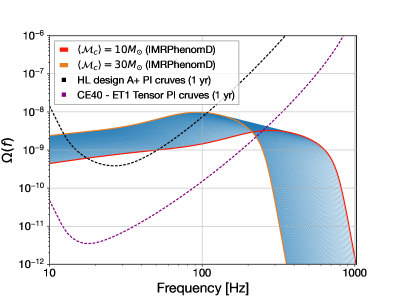
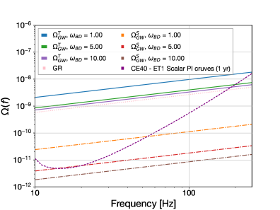
Figure 1: The left panel displays the predicted background spectra constructed using IMRPhenomD for BBH with average chirp mass range of $[10,30]M_{\odot}$ in GR framework. The designed one-year PI curve with the respond of tensor mode for the A+ sensitivity is shown as a dashed black line, while the sensitivity of the network consisting of the CE and ET detectors is depicted as a dashed purple line. The background spectra above these sensitivity curves are generally expected to have a SNR greater than unity. In the right panel, we present the background spectra contribution from BNS, utilizing the frequency-domain inspiral waveforms within the Brans-Dicke theory as described in the text. The tensor and scalar mode backgrounds, corresponding to typical values of $\omega_{BD}=[1,5,10]$, are represented by solid and dash-dotted lines, respectively. For comparison, the background in GR is shown as a dotted line (pink). The prospective one-year PI curve with the respond of sclar mode for the sensitivity of CE and ET networks is depicted by a dashed line (purple), indicating the potential detection of the scalar mode, with SNR $>1$ when the background spectra lies above this line.

4.2 Stochastic signals

Gravitational wave detectors do not measure the GW energy density directly, instead, they measure the GW amplitude at each instrument. Consequently, we need a theory-dependent mapping that relates GW amplitudes to the energy density. One expands the metric perturbation in another useful form for the plane wave expansion,

$$h_{ij}(t,\mathbf{x})=\sum_{A=+,\times,{\rm b}}\int_{-\infty}^{\infty}df\int d^{2}\hat{\mathbf{n}}\tilde{h}_{A}(f,\hat{\mathbf{n}})e_{ij}^{A}(\hat{\mathbf{n}})e^{2\pi if(t-\hat{\mathbf{n}}\cdot\mathbf{x}/c)}.$$ (4.9)

Assuming that the astrophysical gravitational-wave background is stationary, Gaussian, and isotropic, with uncorrelated polarizations, the second moment of the stochastic gravitational wave strain field can be directly expressed in terms of the power spectral density as

$$\left\langle\tilde{h}_{A}^{*}(f,\hat{\mathbf{n}})\tilde{h}_{A^{\prime}}\left(f^{\prime},\hat{\mathbf{n}}^{\prime}\right)\right\rangle=\delta\left(f-f^{\prime}\right)\frac{1}{4\pi}\delta^{2}\left(\hat{\mathbf{n}},\hat{\mathbf{n}}^{\prime}\right)\delta_{AA^{\prime}}\frac{1}{2}S_{A}(f),$$ (4.10)

where the factor of $1/2$ indicates that this equation defines the one-sided power spectral density for each polarization mode. Using the corresponding expression, Eq.(3.7) and Eq.(4.1), one can relate energy densities in each polarization to their strain power-spectral densities via [53]

$$\Omega_{A}(f)=\frac{2\pi^{2}f^{3}}{3H_{0}^{2}}\lambda_{A}(f)S_{A}(f),\quad\lambda_{A}=\begin{cases}\xi^{-1}&\text{ if }A=\mathrm{b},\\ 1&\text{ if }A=+,\times,\end{cases}$$ (4.11)

where $\Omega_{+}$, $\Omega_{\times}$, and $\Omega_{\rm b}$ represent the energy density contributed by plus, cross, and breathing modes. For ground-based GW detectors, it is impractical to directly measure the power spectrum of the polarization amplitudes because the signal is largely dominated by stochastic instrumental and environmental noise [68, 69]. The response $\tilde{h}_{I}(f)$ of the detector $I$ to a passing gravitational wave can be expanded by the antenna patterns $F_{I}^{A}(\hat{n})$ as [70]

$$\tilde{h}_{I}(f)=\int d^{2}\hat{\mathbf{n}}\sum_{A}F_{I}^{A}(\hat{\mathbf{n}})\tilde{h}_{A}(f,\hat{\mathbf{n}})e^{-2\pi if\hat{\mathbf{n}}\cdot\mathbf{x}_{I}/c}$$ (4.12)

In the Fourier domain, the cross-correlation between the outputs of two detectors then can be expressed in terms of the second moment of the distribution of polarization amplitudes as

$$\left\langle\tilde{h}_{I}^{*}(f)\tilde{h}_{J}\left(f^{\prime}\right)\right\rangle=\int d^{2}\hat{\mathbf{n}}~{}d^{2}\hat{\mathbf{n}}^{\prime}\sum_{AA^{\prime}}\left\langle\tilde{h}_{A}^{*}(f,\hat{\mathbf{n}})\tilde{h}_{A^{\prime}}\left(f^{\prime},\hat{\mathbf{n}}^{\prime}\right)\right\rangle$$ (4.13)

$$\times F_{I}^{*A}(\hat{\mathbf{n}})F_{J}^{A^{\prime}}\left(\hat{\mathbf{n}}^{\prime}\right)e^{-2\pi i(f^{\prime}\hat{\mathbf{n}}^{\prime}\cdot\mathbf{x}_{J}/c-f\hat{\mathbf{n}}\cdot\mathbf{x}_{I}/c)},$$

Using the relation between strain power-spectral densities and energy densities in Eq.(4.11) and Eq.(4.10), we would write, instead of Eq.(LABEL:hIhJ),

$$\left\langle\tilde{h}_{I}^{*}(f)\tilde{h}_{J}\left(f^{\prime}\right)\right\rangle=\frac{3H_{0}^{2}}{4\pi^{2}f^{3}}\sum_{A}\lambda^{-1}_{A}(f)\Omega^{A}_{\mathrm{GW}}(f)\gamma^{A}_{IJ}(f)\delta\left(f-f^{\prime}\right),$$ (4.14)

where we have defined the overlap reduction function (ORF) for detectors $I,J$ as

$$\gamma^{A}_{IJ}(f)\equiv\int\frac{d^{2}\hat{\mathbf{n}}}{4\pi}F_{I}^{*A}(\hat{\mathbf{n}})F_{J}^{A}(\hat{\mathbf{n}})e^{2\pi if\hat{\mathbf{n}}\cdot(\mathbf{x}_{I}-\mathbf{x}_{J})}.$$ (4.15)

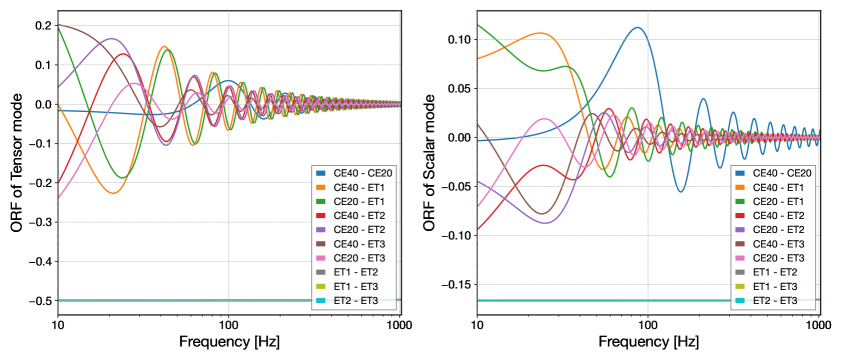
Figure 2: The overlap reduction functions for the tensor mode (left) and the scalar mode (right) in 2CE and ET baselines indicate higher sensitivity to the stochastic background. Apart from the constant overlap reduction function for the three independent interferometers of the ET detector, the overlap reduction functions oscillate around zero, resulting in low sensitivity in such frequency range.

For subsequent data analysis, we will not work directly with $\gamma^{A}_{IJ}(f)$, but instead use the normalized overlap reduction functions as described in [70]. In this case, Eq.(4.14) can be rewrite as:

$$\left\langle\tilde{h}_{I}^{*}(f)\tilde{h}_{J}\left(f^{\prime}\right)\right\rangle=\frac{3H_{0}^{2}}{20\pi^{2}}f^{-3}\delta\left(f-f^{\prime}\right)\times\left[\Omega_{\mathrm{GW}}^{\mathrm{T}}\gamma_{IJ}^{\mathrm{T}}+\lambda^{-1}_{\rm b}\Omega_{\mathrm{GW}}^{\mathrm{S}}\frac{1}{3}\gamma_{IJ}^{\mathrm{S}}\right],$$ (4.16)

where $\Omega_{\mathrm{GW}}^{\mathrm{T}}\equiv\Omega_{\mathrm{GW}}^{+}+\Omega_{\mathrm{GW}}^{\times}$ and $\Omega_{\mathrm{GW}}^{\mathrm{S}}\equiv\Omega_{\mathrm{GW}}^{b}$, respectively.

In Fig. 2, we present the overlap reduction functions for the Cosmic Explorer (CE) and Einstein Telescope (ET) networks. Notably, the ET consists of three separate interferometers positioned at the vertices of an equilateral triangle. The overlap reduction function quantifies the degree of correlation preserved between detectors in the GW signal. The smaller overlap reduction function for the scalar mode compared to the tensor mode indicates that detecting the scalar mode will be more challenging.

5 Simulation and Parameter Estimate

We generated two sets of one-year simulated AGWB data by Pygwb [71]. Based on GR, the first set adopts a fiducial universe and classical populations of BBHs which are consistent with gravitational-wave observations from LIGO-Virgo-KAGRA up to GWTC-3 [72]. This set is used to test the capability of constraining the parameters of BD gravity and the population model. The second set of simulated data is generated using a power-law model, which is fitted to the tensor and scalar gravitational wave energy spectra derived from population models of the BBH and BNS binary systems. This set is designed to explore the potential for detecting scalar gravitational waves with the network of future gravitational wave detectors. For better prospects, we selected our network as {CE40, CE20, ET1} for 2CE and ET detectors. Here, CE40 and CE20 refer to the proposed 40-km and 20-km arm configurations of the CE, respectively, while ET1 represents one of the three objects in proposed triangular configurations for the ET [73].

5.1 Population Models

Recalling the previous sections, the total gravitational wave energy density $\Omega_{\mathrm{GW}}$ depends on the merger rate $\mathcal{R}_{\mathrm{GW}}(z)$ of compact binary coalescences, as well as the energy spectrum $\langle\frac{dE}{df}\rangle_{s}$, which is the function of mass of compact binary.

The merger rate of binary systems is given by the following form [74]:

$$\mathcal{R}_{\mathrm{GW}}(z)=\frac{\mathcal{R}_{0}}{\mathcal{C}}\frac{(1+z)^{\alpha_{z}}}{1+\left(\frac{1+z}{1+z_{p}}\right)^{\alpha_{z}+\beta_{z}}}.$$ (5.1)

Here, $\mathcal{R}_{0}$ is the local rate of binary systems evaluated at redshift $z=0$ and $\mathcal{C}$ is a normalization constant to ensure $\mathcal{R}_{\mathrm{GW}}(0)=\mathcal{R}_{0}$. We adopt parameters $\alpha_{z}=2.7$, $\beta_{z}=2.4$, $z_{p}=2.0$, consistent with Refs [74, 72]. The local rates for the BBHs and BNSs are $\mathcal{R}^{\mathrm{BBH}}_{0}=31\ \mathrm{Gpc}^{-3}\mathrm{yr}^{-1}$ and $\mathcal{R}^{\mathrm{BNS}}_{0}=855\ \mathrm{Gpc}^{-3}\mathrm{yr}^{-1}$, respectively [72]. We truncate the merger rate at $z_{max}=10$, assuming it to be zero at higher redshifts, as the contribution of such distant systems to the overall gravitational wave background is relatively small.

Note that Eq.(4.5) assumes an average chirp mass for all binaries, meaning it does not account for variations in the chirp mass across different binary systems. Given that the total gravitational wave energy density is calculated from the cumulative contributions of various sources, a more general form of Eq.(4.5) is:

$$\frac{dE}{df}|_{s}^{GR}=\langle\mathcal{M}_{c}^{5/3}\rangle\frac{(\pi G)^{2/3}}{3(1+z)^{1/3}}f^{-1/3},$$ (5.2)

where $\langle\mathcal{M}_{c}^{5/3}\rangle$ is determined by the mass distribution of the binary systems. We assume that the masses of BBHs are described by the Power Law + Peak model [75], resulting in $\langle\mathcal{M}_{c}^{5/3}\rangle_{\mathrm{BBH}}=\int\mathcal{M}_{c}^{5/3}p(m_{1},m_{2}|{\bf{\mathrm{\Lambda}_{m}}})dm_{1}dm_{2}$. Here, $p(m_{1},m_{2}|{\bf{\mathrm{\Lambda}_{m}}})$ represents the mass function of this model, with ${\bf{\mathrm{\Lambda}_{m}}}=\left\{\alpha,\beta,m_{\min},m_{\max},\delta_{\rm m},\lambda_{\rm peak},\mu_{\rm m},\sigma_{\rm m}\right\}$ being the (hyper)parameters of the model. To ensure consistency with the distribution described in Ref [72], we adopt the following parameters: $\alpha=3.5$, $\beta=1$, $m_{\min}=5M_{\odot}$, $m_{\max}=80M_{\odot}$, $\delta_{\mathrm{m}}=5M_{\odot}$, $\lambda_{\rm peak}=0.035$, $\mu_{\mathrm{m}}=34M_{\odot}$, and $\sigma_{\mathrm{m}}=5M_{\odot}$. We then obtain $\langle\mathcal{M}_{c}^{5/3}\rangle_{\mathrm{BBH}}=60.8M_{\odot}^{5/3}$, which will be treated as the only free parameter in our Bayesian analysis of the AGWB.

For the BNSs, we simply assume both component masses follow a uniform distribution in (1.2, 2.3) $M_{\odot}$ and are randomly paired, which is consistent with the currently available data [76, 74, 77]. This yields $\langle\mathcal{M}_{c}^{5/3}\rangle_{\rm BNS}=2.0M_{\odot}^{5/3}$. The consideration of BNSs will be used to assess the contribution of scalar GWs to the AWGB.

5.2 Cross-correlation statistic

The cross-correlation of detector pairs is a commonly employed method for detecting the stochastic gravitational-wave background. As shown in Refs [78, 79, 29, 80, 71], at a frequency bin $f$ for a single segment ($i$), the unbiased and minimal-variance optimal estimator for $\Omega_{\mathrm{GW}}$ is given by

$$\hat{C}_{IJ(i)}(f)=\frac{2}{T}\frac{10\pi^{2}}{3H_{0}^{2}}f^{3}\frac{\operatorname{Re}\left[\tilde{s}_{I}^{*}(f)\tilde{s}_{J}(f)\right]}{\gamma_{IJ}(f)}$$ (5.3)

with the corresponding variance:

$$\sigma_{IJ(i)}^{2}(f) =\frac{1}{2Tdf}\left(\frac{10\pi^{2}}{3H_{0}^{2}}\right)^{2}f^{6}P_{I}(f)P_{J}(f).$$ (5.4)

Here, $\tilde{s}_{I(J)}$ denotes the Fourier-transformed strain signal measured by detector $I(J)$, which includes contributions from both gravitational waves and instrumental noise. $T$ is the segment duration, $df$ is the frequency bin width, and $P_{I}(f)$ is the one-sided auto-power spectral density of detector $I$, defined by

$$\left\langle\tilde{s}_{I}^{*}(f)\tilde{s}_{I}\left(f^{\prime}\right)\right\rangle=\frac{1}{2}\delta\left(f-f^{\prime}\right)P_{I}(f).$$ (5.5)

The final estimator and variance are optimally combined by the weighted sum from each segment via [29]

$$\hat{C}_{IJ}(f)=\frac{\sum_{i}\hat{C}_{IJ(i)}(f)\sigma_{IJ(i)}^{-2}(f)}{\sum_{i}\sigma_{IJ(i)}^{-2}(f)},\ \sigma_{IJ}^{-2}(f)=\sum_{i}\sigma_{IJ(i)}^{-2}(f).$$ (5.6)

Here $\hat{C}_{IJ(i)}$ and $\sigma_{IJ(i)}$ denote the individual segment estimators of the detector pairs $IJ$ and their inverse variances, respectively. With the estimate of the SGWB spectrum $\hat{C}_{IJ}(f)$ and variance $\sigma_{IJ}^{2}(f)$, we perform parameter estimation and fit the model. The Gaussian likelihood is formed by combing the spectrum from each baseline $IJ$ as

$$p\left(\hat{C}_{IJ}\mid\bm{\Theta}\right)\propto\exp\left[-\frac{1}{2}\sum_{IJ}\sum_{f}\left(\frac{\hat{C}_{IJ}(f)-\Omega_{\mathrm{GW}}(f,\bm{\Theta})}{\sigma_{IJ}(f)}\right)^{2}\right],$$ (5.7)

where $\Omega_{\mathrm{GW}}(f,\bm{\Theta})$ describes the SGWB model and $\bm{\Theta}$ are its parameters. Given the likelihood, one can estimate the posterior distribution of the parameters of the model using Bayes theorem, $p\left(\bm{\Theta}\mid\hat{C}_{IJ}\right)\propto p\left(\hat{C}_{IJ}\mid\bm{\Theta}\right)p(\bm{\Theta}),$ where $p(\bm{\Theta})$ is the prior distribution on the parameters $\bm{\Theta}$.

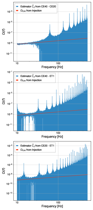
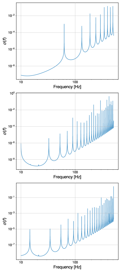
Figure 3: The estimated background spectra, $\hat{C}_{IJ}(f)$, and their corresponding variances, $\sigma_{IJ}^{2}(f)$, derived from three sets of baselines composed of 2CE and ET, are presented in the left (blue) and right panels, respectively. These results are obtained from one-year mock datasets (Dataset I). The fiducial SGWB spectrum (red) is plotted in the left panel for comparison with the estimations.

5.3 Constraints from Waveforms

We first generate a one-year mock datasets (Dataset I) consisting BBH mergers solely. We inject the SGWB signal generated by the fiducial BBH population as described in Sec.5.1 into the baselines, with the corresponding detector noise. As described in Ref [71], the cross-correlation between detectors in our simulations depends on the signal power spectral density (PSD), given our assumption that noise is uncorrelated across all detectors.

With a sampling frequency of 1024 Hz, the simulated dataset from each interferometer is generated in the frequency domain and then transformed into the time domain using the inverse discrete Fourier transform. We split the total time series into intervals and further dividing each interval into segments. This approach reduces the internal storage and computational requirements for the simulation. Finally, we chose 60 segments and each of them contains 256 seconds.

To obtain the power and cross spectra of the detectors for each interval, the segmented time series are Hann-windowed and overlapped by 50% before calculating the Fourier transforms. The resulting spectra are then coarse-grained to a frequency resolution of 1/64 Hz and restricted to the 10-200 Hz frequency band, which contributes most significantly to the expected signal-to-noise ratio. The calculated power and cross spectra for each interval are combined by Eq.(5.6) to obtain the optimal estimator $\hat{C}_{IJ}(f)$ and its corresponding variance $\sigma_{IJ}^{2}(f)$.

Fig. 3 presents the injected SGWB energy density $\Omega_{\mathrm{GW}}(f)$, calculated in GR using the fiducial population and cosmology model. It also shows the corresponding estimator and variance from the baseline in the network of interferometers. The injection of $\Omega_{\mathrm{GW}}(f)$ is well restored, particularly in the frequency band below 100 Hz. Globally, the variance increases with frequency due to the rising noise PSD of the detector. Locally, the sharp increase in variance is attributed to the overlap reduction function oscillating around zero.

Table 1: Parameters and their prior distributions used in the analyses.

Parameter	Description	Fiducial values	Prior
Dataset I
$\langle\mathcal{M}_{c}^{5/3}\rangle\ [M_{\odot}^{5/3}]$	The average of the chirp mass raised to the power of 5/3.	60.8	Uniform $[1,200]$
$\mathrm{Log}_{10}(1/\omega_{BD})$	The logarithm of the reciprocal of the parameter in BD theory.	$-10$	Uniform $[-10,10]$
$\mathcal{R}^{\mathrm{BBH}}_{0}\ [\mathrm{Gpc}^{-3}\mathrm{yr}^{-1}]$	The local BBH merger rate at $z=0$.	$31$	Uniform $[1,100]$
$\alpha_{z}$	The leading slope of the BBH merger rate $\mathcal{R}^{\mathrm{BBH}}(z)$.	$2.7$	Gaussian $(3,1.5)$
$\beta_{z}$	The trailing slope of the BBH merger rate $\mathcal{R}^{\mathrm{BBH}}(z)$.	$2.4$	Gaussian $(1,10)$
$z_{p}$	The peak redshift of the BBH merger rate $\mathcal{R}^{\mathrm{BBH}}(z)$.	$2.0$	Truncated Gaussian $(0.5,4)$ bounded within (0, 30)
Dataset II
$\Omega_{\mathrm{ref}}^{\mathrm{T}}$	The tensor background’s amplitude at 25Hz.	$3.0\times 10^{-9}$	Log-Uniform $[10^{-16},10^{-8}]$
$\alpha_{\mathrm{T}}$	The spectral index of tensor background.	2/3	Uniform $[-3,3]$
$\Omega_{\mathrm{ref}}^{\mathrm{S}}$	The scalar background’s amplitude at 25Hz.	$1.0\times 10^{-11}$	Log-Uniform $[10^{-16},10^{-8}]$
$\alpha_{\mathrm{S}}$	The spectral index of scalar background.	2/3	Uniform $[-3,3]$

To evaluate the capacity of constraining BD gravity, we fix all parameters related to the BBH population for the Bayesian analysis at first, regarding only the BD theory parameter $\omega_{BD}$ is free. We perform Bayesian inference by Bilby [81]. It should be noticed that the simulation is based on GR, therefore we use $\mathrm{Log}_{10}(1/\omega_{BD})$ instead of $\omega_{BD}$ in Bayesian analysis for convenience. GR is recovered as $\mathrm{Log}_{10}(1/\omega_{BD})\rightarrow-\infty$ when $\omega_{BD}\rightarrow+\infty$. However, the value of $\mathrm{Log}_{10}(1/\omega_{BD})=-\infty$ cannot be achieved in analysis. Therefore, we impose a cutoff value $\mathrm{Log}_{10}(1/\omega_{BD})=-10$ as the approximation of GR. Consequently, we choose a uniform prior on $\mathrm{Log}_{10}(1/\omega_{BD})$ at the range of $[-10,10]$. Fig. 4 shows the posterior distribution of $\mathrm{Log}_{10}(1/\omega_{BD})$. The red dotted line denotes the upper limit of $\mathrm{Log}_{10}(1/\omega_{BD})$ at 90% credible level. Converting it to $\omega_{BD}$, we obtain the upper limit is $\omega_{BD}>816.24$ at 90% credible level. It should be pointed that the upper limit exhibits a weak dependence on the cutoff value of the prior for $\mathrm{Log}_{10}(1/\omega_{BD})$. However, a smaller cut-off value for the prior leads to a larger upper limit.

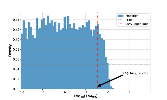
Figure 4: The posterior distribution of $\mathrm{Log}_{10}(1/\omega_{BD})$, assuming that the population properties of BBH are well-constrained and treated as constants. The prior distribution is denoted by the dashed line (grey). The cutoff value of $\mathrm{Log}_{10}(1/\omega_{BD})$ is chosen to be $-10$, corresponding to the recovery of GR. The posterior distribution exhibits weak dependence on the cutoff value. The dotted line (red) indicate the upper limits $\mathrm{Log}_{10}(1/\omega_{BD})=-2.91$ at 90% CL, which implies $\omega_{BD}>816.24$. This constraint is considered highly idealized. More realistic constraints should account for the uncertainty in the population properties of BBH, as illustrated in Fig. 5.

Furthermore, we consider the full parameter space including the BBH population model. For reasonable simplification, we do not consider the individual parameters of the BBH mass distribution. We use $\langle\mathcal{M}_{c}^{5/3}\rangle$ as the representative mass parameter. Thus the parameter space of $\bm{\Theta}$ becomes $\bm{\Theta}=\{\langle\mathcal{M}_{c}^{5/3}\rangle,\ (1/\omega_{BD}),\ \mathcal{R}^{\mathrm{BBH}}_{0},\ \alpha_{z},\ \beta_{z},\ z_{p}\}$. The direct detection of binary black hole mergers provides constraints on the mass distribution, the local merger rate $\mathcal{R}^{\mathrm{BBH}}_{0}$, and the leading slope parameter $\alpha_{z}$ [72, 18, 82, 83]. We adopt slightly narrower priors, aligning with measurements derived from direct detection of binary black hole mergers, compared to those specified in Ref. [32]. These priors are listed in Table 1 in detail. Fig. 5 shows the posterior distributions of the parameters. We effectively recover our prior on the parameters of black holes population. Compared with the last scenario that estimating $\mathrm{Log}_{10}(1/\omega_{BD})$ solely, this case does not provide a more stringent result. Comparing the posterior and prior distributions, we find that $\beta_{\rm z}$ and $z_{\rm p}$ are better constrained, whereas the other parameters for the BBH population are weakly constrained. Fortunately, these parameters (i.e., $\langle\mathcal{M}_{c}^{5/3}\rangle$, $\mathcal{R}^{\mathrm{BBH}}_{0}$, and $\alpha_{z}$) can be better measured by the BBH population analysis [84, 85, 86, 87].

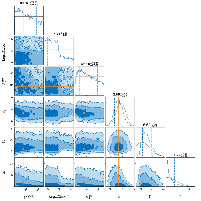
Figure 5: Full posterior distributions obtained by simultaneously inferring the coupling coefficient $\mathrm{Log}_{10}(1/\omega_{BD})$ alongside the population parameters of BBH, i.e., the average mass and the merger rate of BBH. Contour plots depict the $1\sigma$, $2\sigma$, and $3\sigma$ credible regions (blue, light blue, and very light blue, respectively). The grey solid lines in each marginalized posterior illustrate the prior distribution for each parameter. The vertical dashed blue lines represent the $1\sigma$ confidence interval. The injected values, denoted by the orange lines, are recovered within approximately $1\sigma$. Compared to the constraints on the BBH population parameters, the constraint on the BD parameter is relatively weak. In this case, although $\omega_{BD}>1$ holds a high probability, the possibility of $\omega_{BD}<1$ cannot be excluded.

5.4 Seaching for scalar mode

The second one-year simulation dataset (Dataset II) is designed to search for potential scalar gravitational wave background. Different from the the previous one, the second set is generated by a power-law without considering the population properties,

$$\Omega_{\mathrm{GW}}(f)=\Omega_{\mathrm{ref}}^{\mathrm{T}}(\frac{f}{f_{\mathrm{ref}}})^{\alpha_{\mathrm{T}}}+\Omega_{\mathrm{ref}}^{\mathrm{S}}(\frac{f}{f_{\mathrm{ref}}})^{\alpha_{\mathrm{S}}},$$ (5.8)

where $\Omega_{\mathrm{ref}}^{\mathrm{T}}$ and $\Omega_{\mathrm{ref}}^{\mathrm{S}}$ are the reference amplitudes of the tensor and scalar modes at the reference frequency $f_{\mathrm{ref}}=25$ Hz. The spectral indices for the tensor and scalar modes are denoted by $\alpha_{\mathrm{T}}$ and $\alpha_{\mathrm{S}}$, respectively. To illustrate the distinction between the contributions of the scalar and tensor gravitational waves to the stochastic gravitational wave background, we calculate the background energy density $\Omega_{\mathrm{GW}}(f)$ in BD gravity with some typical values of BD parameter. These calculations utilize the population models for BBH and BNS described in Sec.5.1. The corresponding results are presented in Table 2. Given that the scalar gravitational wave arise from the deviations beyond GR, we consider $\omega_{BD}\sim\mathcal{O}(1)$ as an appropriate deviation. The injection values of the parameters are finalized as $\Omega_{\mathrm{ref}}^{\mathrm{T}}=3.0\times 10^{-9}$, $\Omega_{\mathrm{ref}}^{\mathrm{S}}=1.0\times 10^{-11}$, and $\alpha_{\mathrm{T}}=\alpha_{\mathrm{S}}=2/3$. The spectral indices are considered to be $\alpha_{\mathrm{T}}=\alpha_{\mathrm{S}}$, due to the equal sensitivities of compact binaries in both BBH and BNS systems. This equivalence ensures that the energy spectrums do not introduce frequency-dependent corrections that deviate from GR.

The corner plots are displayed in Fig. 6, where we transform the posterior distributions of $\Omega_{\mathrm{ref}}^{\mathrm{T}}$ and $\Omega_{\mathrm{ref}}^{\mathrm{S}}$ into logarithmic space, denoted as $\mathrm{Log}_{10}\Omega_{\mathrm{ref}}^{\mathrm{T}}$ and $\mathrm{Log}_{10}\Omega_{\mathrm{ref}}^{\mathrm{S}}$, respectively. The amplitudes of the tensor mode $\Omega_{\mathrm{ref}}^{\mathrm{T}}$ and the corresponding spectral index $\alpha_{T}$ are recovered within 1$\sigma$. For the search of scalar gravitational waves, the upper limit on the amplitudes is determined to be $\Omega_{\mathrm{ref}}^{\mathrm{S}}<3.064\times 10^{-11}$ (90% CL), corresponding to $\mathrm{Log}_{10}\Omega_{\mathrm{ref}}^{\mathrm{S}}<10.51$ (90% CL), while the spectral index $\alpha_{S}$ remains unconstrained. The weaker constraints on scalar gravitational waves compared to tensor gravitational waves can be attributed to two primary factors. Firstly, the scalar gravitational wave contribute less effect to the stochastic gravitational-wave background intensity than the tensor gravitational waves. Secondly, the ORF of the scalar gravitational wave is smaller than that for tensor gravitational waves, which has been shown in Fig. 2.

Table 2: The background energy density $\Omega_{\mathrm{GW}}(f)$ at 25 Hz for the BBH, BNS, and total background contributions in BD theory, calculated based on the population described in Sec.5.1.

	$\omega_{BD}=1$		$\omega_{BD}=10$		$\omega_{BD}=10000$
	$\Omega_{\mathrm{ref}}^{\mathrm{T}}$(25 Hz)	$\Omega_{\mathrm{ref}}^{\mathrm{S}}$(25 Hz)	$\Omega_{\mathrm{ref}}^{\mathrm{T}}$(25 Hz)	$\Omega_{\mathrm{ref}}^{\mathrm{S}}$(25 Hz)	$\Omega_{\mathrm{ref}}^{\mathrm{T}}$(25 Hz)	$\Omega_{\mathrm{ref}}^{\mathrm{S}}$(25 Hz)
BBH	$4.10\times 10^{-9}$	0	$1.44\times 10^{-9}$	0	$1.18\times 10^{-9}$	0
BNS	$3.86\times 10^{-9}$	$4.47\times 10^{-11}$	$1.31\times 10^{-9}$	$3.40\times 10^{-12}$	$1.07\times 10^{-9}$	$3.20\times 10^{-15}$
Total	$7.96\times 10^{-9}$	$4.47\times 10^{-11}$	$2.75\times 10^{-9}$	$3.40\times 10^{-12}$	$2.25\times 10^{-9}$	$3.20\times 10^{-15}$

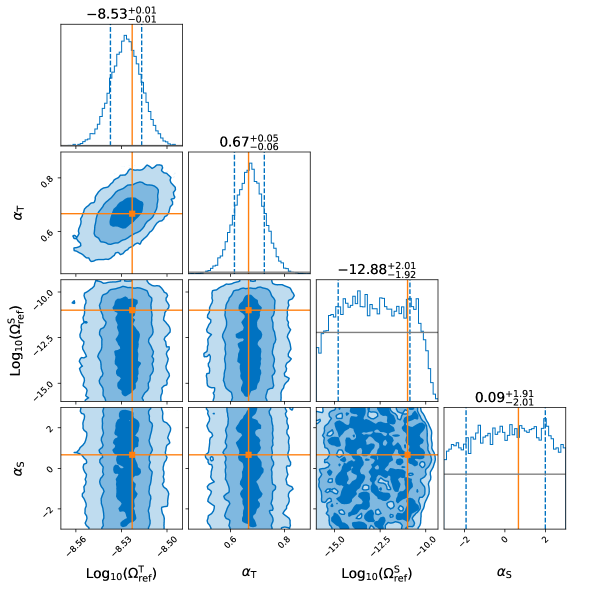
Figure 6: The results of parameter estimation for the one-year simulation dataset (Dataset II) described by the power-law model that includes both tensor and scalar modes. Contour plots depict the $1\sigma$, $2\sigma$, and $3\sigma$ credible regions (blue, light blue, and very light blue, respectively). The grey solid lines represent the prior distributions for each parameter. The tensor mode of the background energy density is tightly constrained, with the amplitude $\Omega_{\mathrm{ref}}^{\mathrm{T}}=(2.95\pm 0.07)\times 10^{-9}$ and the spectral index $\alpha_{\mathrm{T}}=0.67^{+0.05}_{-0.06}$ at the $1\sigma$ credible region. The upper limit on the scalar mode amplitudes of the background energy density is set at $\Omega_{\mathrm{ref}}^{\mathrm{S}}<3.064\times 10^{-11}$ (90% CL). The spectral index of the scalar mode of the background energy density is not significantly constrained.

6 Conclusions

We take Brans-Dicke gravity as an example to comprehensively analyze how the generation and propagation effects of gravitational waveforms under scalar-tensor gravity are encoded into the stochastic gravitational wave background. Unlike previous works that primarily utilized power-law models to search for the stochastic gravitational wave background, or employed Fisher information matrices for parameter estimation, we perform an end-to-end analysis of BD gravity with third-generation gravitational wave detectors. Utilizing realistic population properties of compact binary systems, we generate two sets of one-year astrophysical stochastic gravitational wave background simulation datasets and conducted a complete Bayesian analysis.

The first set of simulations demonstrates that, with well-constrained population parameters, one year of stochastic gravitational wave background observation can provide significant constraints on BD theory. We find that in the best case $\omega_{BD}>816$ at 90% CL. However, the uncertainty of the population properties has a more obvious impact on the stochastic gravitational wave background spectrum than the BD gravity, making it difficult to constrain the theory under such uncertainty. The accurate measurements of the binary population from an increased number of observed systems in third-generation gravitational wave detectors [88], along with extended observation times of the AGWBs, can achieve more stringent constraints on BD gravity. Additionally, by matching waveforms and signals from a larger number of observed binary systems with high SNR, these constraints will be further tightened [89, 90].

The second set of simulations indicates that one year of stochastic gravitational wave observations will yield strong constraints on the tensor mode background, while upper limits can be placed on the scalar mode background, which is two orders of magnitude smaller than the tensor mode background. Besides, the method shows great feasibility to search for scalar modes in the stochastic gravitational wave background. Longer observation times and larger detector networks with more baselines may offer opportunities to detect potential scalar modes.

Due to the fact that the limited observations of NSBHs, the information of their population is inadequate to generate a reliable prospect [72]. We neglect the relatively minor background contributions that may arise from NSBHs. However, the systems of NSBH will provide frequency-dependent corrections in the energy spectrum, offering an opportunity to break the degeneracy with the population and the gravity paramaters. We leave all these prospects and others to future work.

Future space-based gravitational wave detectors, such as the LISA-TianQin networks, will be capable of detecting alternative polarizations of stochastic backgrounds [91]. Moreover, utilizing noise-free correlation measurements from pulsar timing arrays will enhance our understanding of the nanohertz stochastic gravitational wave background, thereby providing deeper insights into gravity [92]. Observations of the stochastic gravitational wave background across a broader range of frequencies will undoubtedly yield more reliable information about gravity.

References

- [1] LIGO Scientific, Virgo collaboration, Observation of Gravitational Waves from a Binary Black Hole Merger, Phys. Rev. Lett. 116 (2016) 061102 [1602.03837].
- [2] LIGO Scientific, Virgo collaboration, GW151226: Observation of Gravitational Waves from a 22-Solar-Mass Binary Black Hole Coalescence, Phys. Rev. Lett. 116 (2016) 241103 [1606.04855].
- [3] LIGO Scientific, Virgo collaboration, GW170817: Observation of Gravitational Waves from a Binary Neutron Star Inspiral, Phys. Rev. Lett. 119 (2017) 161101 [1710.05832].
- [4] LIGO Scientific, Virgo, Fermi-GBM, INTEGRAL collaboration, Gravitational Waves and Gamma-rays from a Binary Neutron Star Merger: GW170817 and GRB 170817A, Astrophys. J. Lett. 848 (2017) L13 [1710.05834].
- [5] LIGO Scientific, Virgo collaboration, GWTC-1: A Gravitational-Wave Transient Catalog of Compact Binary Mergers Observed by LIGO and Virgo during the First and Second Observing Runs, Phys. Rev. X 9 (2019) 031040 [1811.12907].
- [6] LIGO Scientific, Virgo collaboration, GWTC-2: Compact Binary Coalescences Observed by LIGO and Virgo During the First Half of the Third Observing Run, Phys. Rev. X 11 (2021) 021053 [2010.14527].
- [7] KAGRA, VIRGO, LIGO Scientific collaboration, GWTC-3: Compact Binary Coalescences Observed by LIGO and Virgo during the Second Part of the Third Observing Run, Phys. Rev. X 13 (2023) 041039 [2111.03606].
- [8] T. Regimbau, The astrophysical gravitational wave stochastic background, Res. Astron. Astrophys. 11 (2011) 369 [1101.2762].
- [9] E. Thrane and J.D. Romano, Sensitivity curves for searches for gravitational-wave backgrounds, Phys. Rev. D 88 (2013) 124032 [1310.5300].
- [10] N. Christensen, Stochastic Gravitational Wave Backgrounds, Rept. Prog. Phys. 82 (2019) 016903 [1811.08797].
- [11] A.I. Renzini, B. Goncharov, A.C. Jenkins and P.M. Meyers, Stochastic Gravitational-Wave Backgrounds: Current Detection Efforts and Future Prospects, Galaxies 10 (2022) 34 [2202.00178].
- [12] NANOGrav collaboration, The NANOGrav 15 yr Data Set: Evidence for a Gravitational-wave Background, Astrophys. J. Lett. 951 (2023) L8 [2306.16213].
- [13] NANOGrav collaboration, The NANOGrav 15 yr Data Set: Search for Signals from New Physics, Astrophys. J. Lett. 951 (2023) L11 [2306.16219].
- [14] EPTA, InPTA: collaboration, The second data release from the European Pulsar Timing Array - III. Search for gravitational wave signals, Astron. Astrophys. 678 (2023) A50 [2306.16214].
- [15] H. Xu et al., Searching for the Nano-Hertz Stochastic Gravitational Wave Background with the Chinese Pulsar Timing Array Data Release I, Res. Astron. Astrophys. 23 (2023) 075024 [2306.16216].
- [16] P.A. Rosado, Gravitational wave background from binary systems, Phys. Rev. D 84 (2011) 084004 [1106.5795].
- [17] X.-J. Zhu, E. Howell, T. Regimbau, D. Blair and Z.-H. Zhu, Stochastic Gravitational Wave Background from Coalescing Binary Black Holes, Astrophys. J. 739 (2011) 86 [1104.3565].
- [18] KAGRA, Virgo, LIGO Scientific collaboration, Upper limits on the isotropic gravitational-wave background from Advanced LIGO and Advanced Virgo’s third observing run, Phys. Rev. D 104 (2021) 022004 [2101.12130].
- [19] D. Reitze et al., Cosmic Explorer: The U.S. Contribution to Gravitational-Wave Astronomy beyond LIGO, Bull. Am. Astron. Soc. 51 (2019) 035 [1907.04833].
- [20] M. Maggiore et al., Science Case for the Einstein Telescope, JCAP 03 (2020) 050 [1912.02622].
- [21] R. Chen, Y.-Y. Wang, L. Zu and Y.-Z. Fan, Prospects of constraining f(T) gravity with the third-generation gravitational-wave detectors, Phys. Rev. D 109 (2024) 024041 [2401.01567].
- [22] A. Nishizawa and S. Arai, Generalized framework for testing gravity with gravitational-wave propagation. III. Future prospect, Phys. Rev. D 99 (2019) 104038 [1901.08249].
- [23] H. Takeda, A. Nishizawa, K. Nagano, Y. Michimura, K. Komori, M. Ando et al., Prospects for gravitational-wave polarization tests from compact binary mergers with future ground-based detectors, Phys. Rev. D 100 (2019) 042001 [1904.09989].
- [24] A. Addazi et al., Quantum gravity phenomenology at the dawn of the multi-messenger era—A review, Prog. Part. Nucl. Phys. 125 (2022) 103948 [2111.05659].
- [25] A.D. Dolgov and M. Kawasaki, Can modified gravity explain accelerated cosmic expansion?, Phys. Lett. B 573 (2003) 1 [astro-ph/0307285].
- [26] T. Clifton, P.G. Ferreira, A. Padilla and C. Skordis, Modified Gravity and Cosmology, Phys. Rept. 513 (2012) 1 [1106.2476].
- [27] O.H.E. Philcox, Probing parity violation with the four-point correlation function of BOSS galaxies, Phys. Rev. D 106 (2022) 063501 [2206.04227].
- [28] J. Hou, Z. Slepian and R.N. Cahn, Measurement of parity-odd modes in the large-scale 4-point correlation function of Sloan Digital Sky Survey Baryon Oscillation Spectroscopic Survey twelfth data release CMASS and LOWZ galaxies, Mon. Not. Roy. Astron. Soc. 522 (2023) 5701 [2206.03625].
- [29] LIGO Scientific, Virgo collaboration, Search for Tensor, Vector, and Scalar Polarizations in the Stochastic Gravitational-Wave Background, Phys. Rev. Lett. 120 (2018) 201102 [1802.10194].
- [30] A. Maselli, S. Marassi, V. Ferrari, K. Kokkotas and R. Schneider, Constraining Modified Theories of Gravity with Gravitational-Wave Stochastic Backgrounds, Phys. Rev. Lett. 117 (2016) 091102 [1606.04996].
- [31] A. Saffer and K. Yagi, Parameter Estimation for Tests of General Relativity with the Astrophysical Stochastic Gravitational Wave Background, Phys. Rev. D 102 (2020) 024001 [2003.11128].
- [32] T. Callister, L. Jenks, D. Holz and N. Yunes, A New Probe of Gravitational Parity Violation Through (Non-)Observation of the Stochastic Gravitational-Wave Background, 2312.12532.
- [33] P. Brax, C. van de Bruck, A.-C. Davis, J. Khoury and A. Weltman, Detecting dark energy in orbit: The cosmological chameleon, Phys. Rev. D 70 (2004) 123518 [astro-ph/0408415].
- [34] C. Baccigalupi, S. Matarrese and F. Perrotta, Tracking extended quintessence, Phys. Rev. D 62 (2000) 123510 [astro-ph/0005543].
- [35] A. Riazuelo and J.-P. Uzan, Cosmological observations in scalar - tensor quintessence, Phys. Rev. D 66 (2002) 023525 [astro-ph/0107386].
- [36] D. Laya, S. Dutta and S. Chakraborty, Quantum cosmology in coupled Brans–Dicke gravity: A Noether symmetry analysis, Int. J. Mod. Phys. D 32 (2023) 2350001 [2407.06696].
- [37] J.D. Barrow and K.-i. Maeda, Extended inflationary universes, Nucl. Phys. B 341 (1990) 294.
- [38] M. Rossi, M. Ballardini, M. Braglia, F. Finelli, D. Paoletti, A.A. Starobinsky et al., Cosmological constraints on post-Newtonian parameters in effectively massless scalar-tensor theories of gravity, Phys. Rev. D 100 (2019) 103524 [1906.10218].
- [39] J. Solà Peracaula, A. Gómez-Valent, J. de Cruz Pérez and C. Moreno-Pulido, Brans–Dicke cosmology with a -term: a possible solution to CDM tensions, Class. Quant. Grav. 37 (2020) 245003 [2006.04273].
- [40] M. Kramer et al., Strong-Field Gravity Tests with the Double Pulsar, Phys. Rev. X 11 (2021) 041050 [2112.06795].
- [41] A. Errehymy, G. Mustafa, Y. Khedif and M. Daoud, Exploring physical features of anisotropic quark stars in Brans-Dicke theory with a massive scalar field via embedding approach, Chin. Phys. C 46 (2022) 045104.
- [42] C. Brans and R.H. Dicke, Mach’s principle and a relativistic theory of gravitation, Phys. Rev. 124 (1961) 925.
- [43] K.A. Postnov and L.R. Yungelson, The Evolution of Compact Binary Star Systems, Living Rev. Rel. 17 (2014) 3 [1403.4754].
- [44] B. Bertotti, L. Iess and P. Tortora, A test of general relativity using radio links with the Cassini spacecraft, Nature 425 (2003) 374.
- [45] A. Avilez and C. Skordis, Cosmological constraints on Brans-Dicke theory, Phys. Rev. Lett. 113 (2014) 011101 [1303.4330].
- [46] K. Yagi and T. Tanaka, Constraining alternative theories of gravity by gravitational waves from precessing eccentric compact binaries with LISA, Phys. Rev. D 81 (2010) 064008 [0906.4269].
- [47] R. Niu, X. Zhang, B. Wang and W. Zhao, Constraining Scalar-tensor Theories Using Neutron Star–Black Hole Gravitational Wave Events, Astrophys. J. 921 (2021) 149 [2105.13644].
- [48] H. Takeda, S. Tsujikawa and A. Nishizawa, Gravitational-wave constraints on scalar-tensor gravity from a neutron star and black-hole binary GW200115, Phys. Rev. D 109 (2024) 104072 [2311.09281].
- [49] J. Tan and B. Wang, Constraints on Brans-Dicke gravity from neutron star-black hole merger events using higher harmonics, Phys. Rev. D 109 (2024) 084036 [2312.07017].
- [50] C.M. Will, Theory and Experiment in Gravitational Physics (1993).
- [51] M. Maggiore and A. Nicolis, Detection strategies for scalar gravitational waves with interferometers and resonant spheres, Phys. Rev. D 62 (2000) 024004 [gr-qc/9907055].
- [52] D.M. Eardley, D.L. Lee, A.P. Lightman, R.V. Wagoner and C.M. Will, Gravitational-wave observations as a tool for testing relativistic gravity, Phys. Rev. Lett. 30 (1973) 884.
- [53] M. Isi and L.C. Stein, Measuring stochastic gravitational-wave energy beyond general relativity, Phys. Rev. D 98 (2018) 104025 [1807.02123].
- [54] M. Brunetti, E. Coccia, V. Fafone and F. Fucito, Gravitational wave radiation from compact binary systems in the Jordan-Brans-Dicke theory, Phys. Rev. D 59 (1999) 044027 [gr-qc/9805056].
- [55] X. Zhang, J. Yu, T. Liu, W. Zhao and A. Wang, Testing brans-dicke gravity using the einstein telescope, Phys. Rev. D 95 (2017) 124008.
- [56] T. Liu, Y. Wang and W. Zhao, Gravitational waveforms from the inspiral of compact binaries in the brans-dicke theory in an expanding universe, Phys. Rev. D 108 (2023) 024006.
- [57] B. Allen and J.D. Romano, Detecting a stochastic background of gravitational radiation: Signal processing strategies and sensitivities, Phys. Rev. D 59 (1999) 102001 [gr-qc/9710117].
- [58] E.S. Phinney, A Practical theorem on gravitational wave backgrounds, astro-ph/0108028.
- [59] A. Nishizawa, K. Yagi, A. Taruya and T. Tanaka, Cosmology with space-based gravitational-wave detectors — dark energy and primordial gravitational waves —, Phys. Rev. D 85 (2012) 044047 [1110.2865].
- [60] Planck collaboration, Planck 2018 results. VI. Cosmological parameters, Astron. Astrophys. 641 (2020) A6 [1807.06209].
- [61] M. Maggiore, Gravitational Waves. Vol. 1: Theory and Experiments, Oxford University Press (2007), 10.1093/acprof:oso/9780198570745.001.0001.
- [62] I. Kowalska-Leszczynska, T. Regimbau, T. Bulik, M. Dominik and K. Belczynski, Effect of metallicity on the gravitational-wave signal from the cosmological population of compact binary coalescences, Astronomy & Astrophysics 574 (2015) A58.
- [63] LIGO Scientific, Virgo collaboration, Upper Limits on the Rates of Binary Neutron Star and Neutron Star–black Hole Mergers From Advanced Ligo’s First Observing run, Astrophys. J. Lett. 832 (2016) L21 [1607.07456].
- [64] LIGO Scientific, Virgo collaboration, GW170817: Implications for the Stochastic Gravitational-Wave Background from Compact Binary Coalescences, Phys. Rev. Lett. 120 (2018) 091101 [1710.05837].
- [65] Z. Li, Z. Jiang, X.-L. Fan, Y. Chen, L. Gao, Q. Guo et al., Exploring the multiband gravitational wave background with a semi-analytic galaxy formation model, Mon. Not. Roy. Astron. Soc. 527 (2023) 5616 [2304.08333].
- [66] S. Husa, S. Khan, M. Hannam, M. Pürrer, F. Ohme, X. Jiménez Forteza et al., Frequency-domain gravitational waves from nonprecessing black-hole binaries. I. New numerical waveforms and anatomy of the signal, Phys. Rev. D 93 (2016) 044006 [1508.07250].
- [67] S. Khan, S. Husa, M. Hannam, F. Ohme, M. Pürrer, X. Jiménez Forteza et al., Frequency-domain gravitational waves from nonprecessing black-hole binaries. II. A phenomenological model for the advanced detector era, Phys. Rev. D 93 (2016) 044007 [1508.07253].
- [68] LIGO Scientific, Virgo collaboration, Characterization of transient noise in Advanced LIGO relevant to gravitational wave signal GW150914, Class. Quant. Grav. 33 (2016) 134001 [1602.03844].
- [69] LSC collaboration, Identification and mitigation of narrow spectral artifacts that degrade searches for persistent gravitational waves in the first two observing runs of Advanced LIGO, Phys. Rev. D 97 (2018) 082002 [1801.07204].
- [70] A. Nishizawa, A. Taruya, K. Hayama, S. Kawamura and M.-a. Sakagami, Probing non-tensorial polarizations of stochastic gravitational-wave backgrounds with ground-based laser interferometers, Phys. Rev. D 79 (2009) 082002 [0903.0528].
- [71] A.I. Renzini et al., pygwb: A Python-based Library for Gravitational-wave Background Searches, Astrophys. J. 952 (2023) 25 [2303.15696].
- [72] KAGRA, VIRGO, LIGO Scientific collaboration, Population of Merging Compact Binaries Inferred Using Gravitational Waves through GWTC-3, Phys. Rev. X 13 (2023) 011048 [2111.03634].
- [73] “LIGO Document, No. LIGO DCC T1500293-v11.” https://dcc.ligo.org/LIGO-T1500293-v11/public.
- [74] P. Madau and M. Dickinson, Cosmic Star Formation History, Ann. Rev. Astron. Astrophys. 52 (2014) 415 [1403.0007].
- [75] C. Talbot and E. Thrane, Measuring the binary black hole mass spectrum with an astrophysically motivated parameterization, Astrophys. J. 856 (2018) 173 [1801.02699].
- [76] Y.-J. Li, S.-P. Tang, Y.-Z. Wang, M.-Z. Han, Q. Yuan, Y.-Z. Fan et al., Population Properties of Neutron Stars in the Coalescing Compact Binaries, Astrophys. J. 923 (2021) 97 [2108.06986].
- [77] P. Landry and J.S. Read, The Mass Distribution of Neutron Stars in Gravitational-wave Binaries, Astrophys. J. Lett. 921 (2021) L25 [2107.04559].
- [78] LIGO Scientific, VIRGO collaboration, Searching for stochastic gravitational waves using data from the two colocated LIGO Hanford detectors, Phys. Rev. D 91 (2015) 022003 [1410.6211].
- [79] J.D. Romano and N.J. Cornish, Detection methods for stochastic gravitational-wave backgrounds: a unified treatment, Living Rev. Rel. 20 (2017) 2 [1608.06889].
- [80] T. Callister, A.S. Biscoveanu, N. Christensen, M. Isi, A. Matas, O. Minazzoli et al., Polarization-based Tests of Gravity with the Stochastic Gravitational-Wave Background, Phys. Rev. X 7 (2017) 041058 [1704.08373].
- [81] G. Ashton et al., BILBY: A user-friendly Bayesian inference library for gravitational-wave astronomy, Astrophys. J. Suppl. 241 (2019) 27 [1811.02042].
- [82] T.A. Callister and W.M. Farr, Parameter-Free Tour of the Binary Black Hole Population, Phys. Rev. X 14 (2024) 021005 [2302.07289].
- [83] T. Callister, M. Fishbach, D. Holz and W. Farr, Shouts and Murmurs: Combining Individual Gravitational-Wave Sources with the Stochastic Background to Measure the History of Binary Black Hole Mergers, Astrophys. J. Lett. 896 (2020) L32 [2003.12152].
- [84] Y.-J. Li, Y.-Z. Wang, S.-P. Tang and Y.-Z. Fan, Resolving the stellar-collapse and hierarchical-merger origins of the coalescing black holes, 2303.02973.
- [85] Y.-J. Li, S.-P. Tang, S.-J. Gao, D.-C. Wu and Y.-Z. Wang, Exploring field-evolution and dynamical-capture coalescing binary black holes in GWTC-3, 2404.09668.
- [86] S. Rinaldi, W. Del Pozzo, M. Mapelli, A. Lorenzo-Medina and T. Dent, Evidence of evolution of the black hole mass function with redshift, Astron. Astrophys. 684 (2024) A204 [2310.03074].
- [87] W.-H. Guo, Y.-J. Li, Y.-Z. Wang, Y. Shao, S. Wu, T. Zhu et al., The Heavier the Faster: A Sub-population of Heavy, Rapidly Spinning and Quickly Evolving Binary Black Holes, 2406.03257.
- [88] N. Singh, T. Bulik, K. Belczynski and A. Askar, Exploring compact binary populations with the Einstein Telescope, Astron. Astrophys. 667 (2022) A2 [2112.04058].
- [89] M. Punturo et al., The Einstein Telescope: A third-generation gravitational wave observatory, Class. Quant. Grav. 27 (2010) 194002.
- [90] X. Zhang, J. Yu, T. Liu, W. Zhao and A. Wang, Testing Brans-Dicke gravity using the Einstein telescope, Phys. Rev. D 95 (2017) 124008 [1703.09853].
- [91] Y. Hu, P.-P. Wang, Y.-J. Tan and C.-G. Shao, Testing the polarization of gravitational wave background with LISA-TianQin network, 2209.07049.
- [92] R.C. Bernardo and K.-W. Ng, Testing gravity with cosmic variance-limited pulsar timing array correlations, Phys. Rev. D 109 (2024) L101502 [2306.13593].