Abstract

This paper examines the impact of discrete marginal distributions on copula-based Markov chains. We present results on mixing and parameter estimation for a copula-based Markov chain model with Bernoulli($p$) marginal distribution and highlight the differences between continuous and discrete state-space Markov chains. We derive estimators for model parameters using the maximum likelihood approach and discuss other estimators of $p$ that are asymptotically equivalent to its maximum likelihood estimator. The asymptotic distributions of the parameter estimators are provided. A simulation study showcases the performance of the different estimators of $p$. Additionally, statistical tests for model parameters are included.

Keywords Asymptotic normality $\cdot$ Dependent Bernoulli trials $\cdot$ Frechet family of copulas $\cdot$ Mixing for Markov chains

1 Introduction

Markov chain models have been widely used in the literature to represent the relationship between consecutive observations in a sequence of Bernoulli trials. Johnson and Klotz (1974) [1] employed a Markov chain generalization of a binomial model to analyze the crystal structure of a two-metal alloy in their metallurgical studies. Crow (1979) [2] investigated the applications of two-state Markov chains in telecommunications in his study focusing on approximating confidence intervals. Brainerd and Chang (1982) [3] utilized two-state Markov chains to address problems in linguistic analysis. These examples illustrate that Markov chain models can provide a solid foundation for modeling a wide range of two-state sequential phenomena.

Moreover, in the study of sequences consisting of different alternatives, there has been notable interest in using group or run tests to evaluate the randomness of the sequences. These tests are based on the count of changes between outcomes in the sequence, aiming to assess whether the sequence displays randomness (denoted as the null hypothesis, $H_{0}$) or exhibits a type of dependence similar to simple Markov chains (alternative hypothesis, $H_{1}$). These counts, denoted by $n_{ij}\ (\text{where}\ i,j=0,\cdots,s\ \text{denotes the states taken by the sequence})$ are commonly referred to as transition numbers of the sequence. The transition numbers have been widely used in literature to construct run tests and in estimation of model parameters (see David (1947b) [4], Goodman (1958) [5], Anderson and Goodman (1957) [6] and Billingsley (1961a) [7] for details). As used in this work, transition numbers prove to be very useful in computing the maximum likelihood estimators of parameters.

1.1 Copulas and Markov chains

A 2-copula is a bivariate function $C:[0,1]^{2}\rightarrow[0,1]$ such that $C(0,u)=C(u,0)=0$, $C(u,1)=C(1,u)=u,\forall\ u\in[0,1]$ and $C(u_{1},v_{1})+C(u_{2},v_{2})-C(u_{1},v_{2})-C(u_{2},v_{1})\geq 0,\forall\ [u_{1},u_{2}]\times[v_{1},v_{2}]\subset[0,1]^{2}$. For some $k\geq 2,$ let $C_{1},\cdots,C_{k}$ be a set of $k$ copulas and $a_{1},\cdots,a_{k}$ a set of real constants such that $a_{1}+\cdots+a_{k}=1$ and $0\leq a_{i}\leq 1$ for each $i=1,\cdots,k$, then the sum given by $C(u,v)=a_{1}C_{1}(u,v)+\cdots+a_{k}C_{k}(u,v)$ is a copula referred to as the convex combination of $C_{1},\cdots,C_{k}$ (Longla, 2015) [8].

In the recent past, copulas have gained popularity in the modeling of temporal dependence within Markov processes (Nelsen (2006) [9]). This is because, when used to represent joint distributions of random variables, they enable the detection of possible correlations or links between variables (Darsow, Nguyen and Olsen (1992) [10]). A copula-based Markov chain is a stationary Markov chain generated by the copula of its consecutive states and an invariant distribution. Copula-based Markov chains enable the exploration of dependence and mixing properties inherent in Markov processes. This makes them an invaluable tool for investigations and allows for the study of scale-free measures of dependence while remaining invariant under monotonic transformations of the variables. Consequently, copula methods have drawn a lot of interest across diverse fields, including technology, finance, and the natural world.

This paper focuses on a stationary Markov chain based on a copula from the Frechet family of copulas. We study two cases: a continuous state-space Markov chain with uniform marginal distribution and a discrete state-space Markov chain with Bernoulli($p$) marginal distribution. Maximum likelihood estimators (MLEs) of model parameters are derived in both cases and their asymptotic distributions are provided. The likelihood ratio test is used to test for randomness in the model.

Studies involving inferential statistics for discrete cases closely similar to the one considered here have been presented in the works of Billingsley (1961a) [7], Billingsley (1961b) [11], Goodman (1958) [5], Klotz (1972) [12], Klotz (1973) [13], Price (1976) [14], Lindqvist (1978) [15], and others. Billingsley (1961a) [7] based his theory on the $\chi^{2}$ method and the Neyman-Pearson criterion. Goodman (1958) [5] considered a single sequence of alternatives consisting of a long chain of observations to derive some long sequence group tests. Klotz (1973) [13] presented small and large sample distribution theory for the sufficient statistics of a model for Bernoulli trials with Markov dependence. He provided estimators for the model parameters and showed that the uniform most powerful (u.m.p.) unbiased test of independence is the run test. On the other hand, Price (1976) [14] and Lindqvist (1978) [15] focused on estimating the model parameters only. Price (1976) [14] used Monte Carlo techniques to investigate finite sample properties for the parameters of a dependent Bernoulli process. Lindqvist (1978) [15] considered the weaker assumption of non-Markovian dependence and showed that the MLE, $(\hat{p},\hat{a})$ is a strongly consistent, and asymptotically normally distributed estimator for $(p,a)$. In this context, $p$ represents the Bernoulli (frequency) parameter, while $a$ is an additional dependence parameter. He further showed that $(\hat{p},\hat{a})$ is asymptotically equivalent to $(\bar{p},\bar{a})$, where $\bar{p}$ is the sample mean and $\bar{a}$ is the empirical correlation coefficient of $X_{t-1}$ and $X_{t}$.

The rest of the paper is organized as follows: In Section 2, we introduce our model and detail the transition probabilities of the discrete Markov chain model considered. Mixing properties of the Markov chain model are discussed in Subsection 2.1. Section 3 covers parameter estimation, where we derive MLEs and their asymptotic distributions. In Section 4 we provide a test for independence in the sequence. The paper concludes with a simulation study in Section 5.

2 The model

Consider a stationary Markov chain model based on the copula

$$C(u,v)=aM(u,v)+(1-a)W(u,v),\qquad a\in(0,1).$$ (2.1)

The copula (2.1) is from the Frechet/Mardia family of copulas (for details on these copula families, see Nelsen (2006) [9], Joe (1997) [16], or Durante and Sempi (2015) [17]).

Longla (2014) [18] showed that a stationary Markov chain generated by the copula (2.1) and uniform marginals has $n$-steps joint cumulative distribution function of the form $C_{n}(u,v)=1/2[1+(2a-1)^{n}]M(u,v)+1/2[1-(2a-1)^{n}]W(u,v).$

If the marginals are Bernoulli($p$), the joint distributions can be characterized by the transition probabilities of the Markov chain and the stationary distribution. Theorem (1) below provides the transition matrices for the Markov chain.

Theorem 1.

Let $X=(X_{t})_{t=0,\cdots,n}$ be a stationary Markov chain generated by copula (2.1) and Bernoulli($p$) marginals. Then $X$ has transition matrices given by

$$A=\begin{pmatrix}\frac{ap+1-2p}{1-p}&\frac{p(1-a)}{1-p}\\ 1-a&a\end{pmatrix},\ p<1/2$$ (2.2)

and

$$A=\begin{pmatrix}a&1-a\\ \frac{(1-p)(1-a)}{p}&\frac{a(1-p)+2p-1}{p}\\ \end{pmatrix},\ p\geq 1/2.$$ (2.3)

Proof.

Due to stationarity of the Markov chain, $P(X_{t}=1)=1-P(X_{t}=0)=p$. It suffices to determine $P(X_{0}=0,X_{1}=0)$.

$$P(X_{0}=0,X_{1}=0) =P(X_{0}\leq 0,X_{1}\leq 0)=C(1-p,1-p)$$

$$=a(1-p)+(1-a)\max(1-2p,0)$$

$$=\begin{cases}ap+1-2p,&\quad\quad\text{if}\ p<1/2\\ a(1-p),&\quad\quad\text{if}\ p\geq 1/2,\end{cases}$$

where the second equality follows from Sklar’s Theorem (Sklar (1959)) [19]. The rest of the probabilities are computed using the hypothesis that the Markov chain is stationary with Bern(p) marginals. For $p<1/2$, the joint distribution is given by Table 1 below.

	0	1	$P_{X_{0}}(x)$
0	$ap+1-2p$	$p(1-a)$	$1-p$
1	$p(1-a)$	$ap$	$p$
$P_{X_{1}}(y)$	$1-p$	$p$	1

Table 1: Distribution of $(X_{0},X_{1})$ when $p<1/2.$

Using the definition of conditional probability, $P(X_{1}=j|X_{0}=i)=P(X_{1}=j,X_{0}=i)/P(X_{0}=i)$, in Table 1 we obtain the transition matrix (2.2). A similar argument is used for $p\geq 1/2$ to get the transition matrix (2.3). ∎

The statistical behavior of the distribution at $p=1/2$ reflects a symmetric transition structure where the probability of transitioning between states is balanced by the parameter $a$. This symmetry simplifies the interpretation and analysis of the Markov chain, making it an interesting case for studying the dynamics governed by the mixture copula model.

The transition matrix (2.2) is similar to the one considered by Klotz (1973) [13]. In our case, $p=P(X_{t}=1)$ is the usual frequency parameter and $a=P(X_{t}=1|X_{t-1}=1)$, when $p<1/2$ or $a=P(X_{t}=0|X_{t-1}=0)$, when $p\geq 1/2$ is the dependence parameter. In Klotz (1973) [13], the condition $\max(0,(2p-1)/p)\leq a\leq 1$ was required so that the transition probabilities of the model remain bounded between $0$ and $1$. The model presented in this work does not require this condition because the copula conditions sufficiently define the transition probabilities based on whether $p<1/2$ or $p\geq 1/2$. Specifically, the transition probabilities remain bounded between 0 and 1 for any value of $0<a<1$, and they satisfy $\sum\limits_{j}p_{ij}=1$ for $j=0,1$.

Proposition 2.

The $n^{th}$ transition matrices for (2.2) and (2.3) are respectively

$$A^{n}=\begin{pmatrix}1-p+p(\frac{a-p}{1-p})^{n}&p-p(\frac{a-p}{1-p})^{n}\\ 1-p-(1-p)(\frac{a-p}{1-p})^{n}&p+(1-p)(\frac{a-p}{1-p})^{n}\end{pmatrix},\quad\quad p<1/2$$ (2.4)

and

$$A^{n}=\begin{pmatrix}1-p+p\left(\frac{a+p-1}{p}\right)^{n}&p-p\left(\frac{a+p-1}{p}\right)^{n}\\ 1-p-(1-p)\left(\frac{a+p-1}{p}\right)^{n}&p+(1-p)\left(\frac{a+p-1}{p}\right)^{n}\end{pmatrix},\quad\quad p\geq 1/2$$ (2.5)

Proof.

For $p<1/2$, the eigenvalues of $A$ are obtained by solving the characteristic equation:

$$\lambda^{2}-\frac{a+1-2p}{1-p}\lambda+\frac{a-p}{1-p}=0.$$

Solving this equation yields $\lambda_{1}=1$ and $\lambda_{2}=\frac{a-p}{1-p}$. Then,

$$A^{n}=\begin{pmatrix}a_{00}+b_{00}\lambda_{2}^{n}&a_{01}+b_{01}\lambda_{2}^{n}\\ a_{10}+b_{10}\lambda_{2}^{n}&a_{11}+b_{11}\lambda_{2}^{n}\end{pmatrix},$$ (2.6)

where $a_{ij}$, $b_{ij}$, $i,j=0,1$ are coefficients to be determined, and $\lambda_{2}$ is the non-simple eigenvalue of $A$. By using (2.6) to write $A^{0}$ and $A^{1}$, we can solve for $a_{ij}$ and $b_{ij}$, $i,j=0,1$, by forming four simultaneous equations, which are easy to solve. This yields the $n^{th}$ transition matrix (2.4). Similar steps are used to obtain the $n^{th}$ transition matrix for (2.3). ∎

2.1 Mixing

Most of the dependence and mixing coefficients are heavily influenced by the copula of the model of interest (Longla and Peligrad (2012) [20]). Longla (2014) [18] proposed a set of copula families that generate exponential $\rho$-mixing Markov chains. He showed that stationary Markov chains generated by copulas from the the Frechet(Mardia) families and uniform marginals are exponentially $\phi$-mixing, therefore $\rho$-mixing and geometrically $\beta$-mixing if $a+b\neq 1$. However, when $a+b=1$, mixing does not occur (Longla, 2014) [18]. Furthermore, Longla (2015) [8] showed that copulas from these families fail to generate $\psi$-mixing continuous state-space strictly stationary Markov chains for any $a$ and $b$, achieving at best ‘lower $\psi$-mixing’. Longla (2015) [8] also noted the absence of $\psi$-mixing for copulas from Mardia and Frechet families for any $a$ and $b$. Different results emerge when discrete marginal distributions are employed.

We define two mixing coefficients in this paper: the $\phi$-mixing coefficient, introduced by Ibragimov (1959) [21] and further studied by Cogburn (1960) [22], and the $\psi$-mixing coefficient, first introduced by Blum, Hanson, and Koopmans (1963) [23] and refined by Philip (1969) [24]. In the context of a probability space $(\Omega,\mathcal{F},P)$ with sigma algebras $\mathcal{A},\mathcal{B}\subset\mathcal{F}$, the coefficients are defined in literature as follows (see Bradley (2007) [25])

$$\phi(\mathcal{A},\mathcal{B})=\sup_{A\in\mathcal{A},B\in\mathcal{B},P(A)>0}\left|\frac{P(B\cap A)}{P(A)}-P(B)\right|,$$

$$\psi(\mathcal{A},\mathcal{B})=\sup_{A\in\mathcal{A},B\in\mathcal{B},P(A)>0,P(B)>0}\left|\frac{P(A\cap B)}{P(A)P(B)}-1\right|.$$

For random variables $n$-steps apart such that $X_{0}\in A$ and $X_{n}\in B$, we define the mixing coefficients

$$\phi(n)=\sup\limits_{A\in\mathcal{A},B\in\mathcal{B},P(A)>0}\left|\frac{P^{n}(B\cap A)}{P(A)}-P(B)\right|,\quad$$ (2.7)

$$\psi(n)=\sup\limits_{A\in\mathcal{A},B\in\mathcal{B},P(A)>0,P(B)>0}\left|\frac{P^{n}(A\cap B)}{P(A)P(B)}-1\right|,\quad$$ (2.8)

where $P^{n}(A\cap B)=P(X_{0}\in A,X_{n}\in B)$. A random process is said to be $\psi-$mixing if $\psi(n)\longrightarrow 0\ \text{as}\ n\longrightarrow\infty$ and $\phi-$mixing if $\phi(n)\longrightarrow 0\ \text{as}\ n\longrightarrow\infty$. For the case involving discrete state-space Markov chains generated by the copula given by (2.1) and Bernoulli$(p)$ marginal distribution, we establish the following theorem:

Theorem 3.

Let $X=(X_{t})_{t=0,\cdots,n}$ be a stationary Markov chain generated by copula (2.1) and Bernoulli($p$) marginal distributions. Then $X$ is exponential $\psi$-mixing, and hence also exponential $\phi$, $\rho$, $\beta$ and $\alpha$-mixing.

Proof.

Consider the coefficient defined by Equation (2.8) with $\Omega=\{0,1\}$. For $p<1/2$, we examine

$$\left|\frac{P^{n}(A\cap B)}{P(A)P(B)}-1\right|,$$

where $A$ and $B$ are chosen only from $\{0\}$ or $\{1\}$ since $P(\{0,1\}\cap A)=P(A)$. The joint distribution of $(X_{0},X_{n})$ when $p<1/2$ is obtained from the $n^{th}$ transition matrix (2.4) and using $P(X_{1}=j,X_{0}=i)=P(X_{1}=j|X_{0}=i)P(X_{0}=i)$. This is given in Table 2.

	0	1	$P_{X_{0}}(x)$
0	$(1-p)^{2}+p(1-p)(\frac{a-p}{1-p})^{n}$	$p(1-p)-p(1-p)(\frac{a-p}{1-p})^{n}$	$1-p$
1	$p(1-p)-p(1-p)(\frac{a-p}{1-p})^{n}$	$p^{2}+p(1-p)(\frac{a-p}{1-p})^{n}$	p
$P_{X_{n}}(y)$	$1-p$	$p$	1

Table 2: Distribution of $(X_{0},X_{n})$ when $p<1/2.$

After computing the four quantities,

$$|\frac{P(X_{0}=i,X_{n}=j)}{P(X_{0}=i)P(X_{n}=j)}-1|$$

from Table 2 we end up with

$$\psi(n) =\sup\{\frac{p}{1-p}\left|\frac{a-p}{1-p}\right|^{n},\left|\frac{a-p}{1-p}\right|^{n},\frac{1-p}{p}\left|\frac{a-p}{1-p}\right|^{n}\}=\frac{1-p}{p}\left|\frac{a-p}{1-p}\right|^{n}$$

For $p\geq 1/2$, a similar argument leads to $\psi(n)=\frac{p}{1-p}\left|\frac{a+p-1}{p}\right|^{n}.$ Therefore, for all $a,p\in(0,1)$, $\psi(n)\longrightarrow 0\ \text{at an exponential rate as}\ n\longrightarrow\infty$. ∎

3 Parameter estimation asymptotic normality

The characteristics of the model parameter estimators, including the shape of their asymptotic distributions, rely on the chosen marginal distribution.

3.1 Markov chain with uniform marginals

Assuming $(X_{t})_{t=0,\cdots,n}$ is a Markov chain generated by copula (2.1) with uniform$(0,1)$ marginal distribution and utilizing Sklar’s theorem, the joint cumulative distribution function of $(X_{t},X_{t+1})$ is represented as:

$$F(x_{t},x_{t+1})=C(F(x_{t}),F(x_{t+1}))=aM(x_{t},x_{t+1})+(1-a)W(x_{t},x_{t+1}).$$ (3.1)

The copulas $M$ and $W$ have support on the main diagonal and secondary diagonal of $[0,1]^{2}$ respectively (Nelsen (2006) [9]). The joint distribution (3.1) implies $P(X_{t}=X_{t+1})=a$ and $P(X_{t}=1-X_{t+1})=1-a$ due to the properties of mixture distributions. The indicator random variable $I(X_{t}=X_{t+1}),\ t\in{0,1,\ldots,n-1}$, taking the value $1$ when $X_{t}=X_{t+1}$ and $0$ otherwise, follows a Bernoulli($a$) distribution with probability of success $a$ and probability of failure $1-a$. The parameter $a$ can be estimated by the sample mean:

$$Y_{n}=\frac{1}{n}\sum_{t=0}^{n-1}I(X_{t}=X_{t+1})$$ (3.2)

as demonstrated in Proposition (4) below.

Proposition 4.

Let $(X_{t})_{t=0,\cdots,n}$ be a Markov chain generated by copula (2.1) and the uniform(0,1) distribution. We have the following:

• The random variables $I(X_{t}=X_{t+1}),t=0,\cdots,n-1$ are independent and identically distributed (i.i.d) Bernoulli random variables.

• The random variable (3.2) is an unbiased and consistent estimator of $a$. Moreover, $Y_{n}$ satisfies the Central Limit Theorem.

• The MLE of $a$ is the method of moments estimator given by (3.2).

Proof.

• We establish independence in the sequence via induction. For two random variables$(m=2)$, consider, without loss of generality, the variables $I(X_{1}=X_{0})$ and $I(X_{2}=X_{1})$. We demonstrate that the joint probability $P(X_{1}=X_{0},X_{2}=X_{1})$ equals $P(X_{1}=X_{0})P(X_{2}=X_{1})$.

  $$P(X_{1}= X_{0},X_{2}=X_{1})=\int\int P(X_{1}=X_{0},X_{2}=X_{1}|X_{0}=x,X_{1}=x)dP_{X_{0}}(x)dP_{X_{1}}(x)$$

  $$=\int\int P(X_{1}=x,X_{2}=x|X_{0}=x,X_{1}=x)dP_{X_{0}}(x)dP_{X_{1}}(x)\ \text{(this follows by }$$

        applying the definition of conditional probability and rearranging

        terms)

  $$=\int\int P(X_{1}=x|X_{0}=x,X_{1}=x,X_{2}=x)P(X_{2}=x|X_{0}=x,X_{1}=x)dP_{X_{0}}(x)$$

  $$\qquad\qquad\qquad\qquad\ dP_{X_{1}}(x)\text{ (by the multiplication rule for probabilities)}$$

  $$=\int\int P(X_{1}=x|X_{0}=x)P(X_{2}=x|X_{1}=x)dP_{X_{0}}(x)dP_{X_{1}}(x)\ \text{(by the Markov }$$

        property)

  $$=\int P(X_{1}=x|X_{0}=x)dP_{X_{0}}(x)\int P(X_{2}=x|X_{1}=x)dP_{X_{1}}(x)\ \text{(separating the}$$

        integrals)

  $$=P(X_{1}=X_{0})P(X_{2}=X_{1})\ \text{( integrating out $X_{0}$ and $X_{1}$).}$$

  Hence it follows that

  $$P(X_{1}=X_{0},X_{2}=X_{1})=P(X_{1}=X_{0})P(X_{2}=X_{1})$$ (3.3)

  Suppose independence holds for $m=k>2$ indicator variables.

  $$P(X_{1}=X_{0},X_{2}=X_{1},\cdots,X_{k+1}=X_{k})=\prod\limits_{i=0}^{k}P(X_{i+1}=X_{i}).$$ (3.4)

  Let $m=k+1$. Then

  $$P(X_{1} =X_{0},X_{2}=X_{1},\cdots,X_{k+1}=X_{k},X_{k+2}=X_{k+1})$$

  $$=P(X_{k+2}=X_{k+1}|X_{k+1}=X_{k},\cdots,X_{2}=X_{1},X_{1}=X_{0})\times$$

  $$\qquad P(X_{1}=X_{0},X_{2}=X_{1},\cdots,X_{k+1}=X_{k})\ \text{(by multiplication rule}$$

  of probabilities)

  $$=P(X_{k+2}=X_{k+1}|X_{k+1}=X_{k})\times\prod\limits_{i=0}^{k}P(X_{i+1}=X_{i})\ \text{(by the Markov }$$

  property and (3.4) above)

  $$=\prod\limits_{i=0}^{k+1}P(X_{i+1}=X_{i})\ \text{(due to (\ref{indep for pair})).}$$

• The proof follows from the properties of the estimator of the Bernoulli parameter for an i.i.d. Bernoulli(a) sample.

• Let $Y_{t}=I(X_{t}=X_{t+1})$,

  $$L(X_{t},X_{t+1})=a^{Y_{t}}(1-a)^{1-Y_{t}}.$$ (3.5)

  The likelihood function is

  $$L(a)=\prod\limits_{t=0}^{n-1}L(X_{t},X_{t+1})=a^{\sum_{t=0}^{n-1}Y_{t}}(1-a)^{n-\sum_{t=0}^{n-1}Y_{t}}.$$ (3.6)

  It follows that $\hat{a}=\frac{1}{n}\sum_{t=0}^{n-1}Y_{t}=\frac{1}{n}\sum_{t=0}^{n-1}I(X_{t}=X_{t+1})$.

∎

3.2 Stationary Markov chain with Bern$(p)$ marginal distribution.

The literature has extensively discussed the statistical inference for finite Markov chains. When transition probabilities of the Markov chain are expressed as $p_{ij}(\boldsymbol{\theta})$, with ${\boldsymbol{\theta}}=(\theta_{{1}},\cdots,\theta{r})$, the log-likelihood is $\sum_{ij}n_{ij}\log p_{ij}(\boldsymbol{\theta})$ (see Billingsley (1961a) [7] and Billingsley (1961b) [11]). If the $r$ components of $\boldsymbol{\theta}$ are all real, then the maximum likelihood equations are

$$\sum_{ij}\frac{n_{ij}}{p_{ij}(\boldsymbol{\theta})}\frac{\partial p_{ij}(\boldsymbol{\theta})}{\partial\theta_{u}}=0,\ u=0,1,\cdots,r.$$ (3.7)

Considering the transition matrix (2.2) for instance, the likelihood function of the sample is

$$L(\boldsymbol{\theta})=p^{x_{0}}(1-p)^{1-x_{0}}\left(\frac{ap+1-2p}{1-p}\right)^{n_{{}_{00}}}\left(\frac{p(1-a)}{1-p}\right)^{n_{{}_{01}}}(1-a)^{n_{{}_{10}}}a^{n_{{}_{11}}}$$ (3.8)

and the log-likelihood is given by

$$\begin{split}\mathcal{L}(\boldsymbol{\theta})=\log L(\boldsymbol{\theta})=&x_{0}\log(p)+(1-x_{0})\log(1-p)+n_{00}\log(ap+1-2p)-\\ &n_{00}\log(1-p)+n_{01}\log(p)+n_{01}\log(1-a)-n_{01}\log(1-p)\\ &\qquad+n_{10}\log(1-a)+n_{11}\log(a).\end{split}$$ (3.9)

Differentiating (3.9) with respect to $a$ and $p$ gives

$$\begin{cases}&\frac{\partial\mathcal{L}(\boldsymbol{\theta})}{\partial a}=\frac{n_{{}_{00}}p}{ap+1-2p}-\frac{n_{{}_{01}}}{1-a}-\frac{n_{{}_{10}}}{1-a}+\frac{n_{11}}{a}=0\\ &\frac{\partial\mathcal{L}(\boldsymbol{\theta})}{\partial p}=\frac{x_{0}}{p}-\frac{1-x_{0}}{1-p}+\frac{n_{{}_{00}}(a-2)}{ap+1-2p}+\frac{n_{{}_{00}}}{1-p}+\frac{n_{{}_{01}}}{p}+\frac{n_{{}_{01}}}{1-p}=0.\end{cases}$$ (3.10)

The equations in (3.10) can be rewritten in the form

$$\begin{cases}&npa^{2}-[(2n-n_{{}_{00}}+n_{{}_{11}})p-n+n_{{}_{00}}]a+n_{{}_{11}}(2p-1)=0\\ &a[x_{0}p-p^{2}+n_{{}_{00}}p+n_{{}_{01}}p]+x_{0}-2x_{0}p-p+2p^{2}-n_{{}_{00}}p+n_{{}_{01}}-2n_{{}_{01}}p=0.\end{cases}$$ (3.11)

Solving for $a$ in the second equation of (3.11) gives

$$\hat{a}=\frac{p(\lambda_{1}-2p)-\lambda_{2}}{p(\lambda_{3}-p)},$$ (3.12)

where $\lambda_{1}=2x_{0}+1+n_{{}_{00}}+2n_{{}_{01}},\lambda_{2}=x_{0}+n_{{}_{01}}$ and $\lambda_{3}=x_{0}+n_{{}_{00}}+n_{{}_{01}}.$ Substituting (3.12) for $a$ in the first equation of (3.11) and using $\lambda_{4}=2n-n_{{}_{00}}+n_{{}_{11}},$ and $\lambda_{5}=n-n_{{}_{00}}$ we obtain

$$(4n-2\lambda_{4} +2n_{{}_{11}})p^{4}+(2\lambda_{3}\lambda_{4}-4n\lambda_{1}+\lambda_{1}\lambda_{4}+2\lambda_{5}-n_{{}_{11}}-4n_{{}_{11}}\lambda_{3})p^{3}+$$

$$(n\lambda_{1}^{2}+4n\lambda_{2}-\lambda_{1}\lambda_{3}\lambda_{4}-\lambda_{2}\lambda_{4}-2\lambda_{3}\lambda_{5}-\lambda_{1}\lambda_{5}+2n_{{}_{11}}\lambda_{3}+2n_{{}_{11}}\lambda_{3}^{2})p^{2}+$$

$$(\lambda_{1}\lambda_{3}\lambda_{5}-2n\lambda_{1}\lambda_{2}+\lambda_{2}\lambda_{3}\lambda_{4}+\lambda_{2}\lambda_{5}-n_{{}_{11}}\lambda_{3}^{2})p+(n\lambda_{2}^{2}-\lambda_{2}\lambda_{3}\lambda_{5})=0,$$ (3.13)

There is no closed-form solution for equation (3.2) but numerical solutions can be obtained.

The sufficient conditions for MLEs and their asymptotic properties are specified in Condition 5.1 of Billingsley (1961a) [7], as presented below.

Condition 5.

Let $X=(X_{t})_{t=0,\cdots,n}$ be a Markov chain with finite state space $S=\{0,\cdots,s\}$. Suppose $P=(p_{ij}(\boldsymbol{\theta}))$ is the $s\times s$ stochastic matrix, where ${\boldsymbol{\theta}}=(\theta_{{}_{1}},\cdots,\theta_{r})$ ranges over an open subset $\Theta$ of $\mathbb{R}^{r}$. Suppose that the following conditions are satisfied:

• The set $E$ of $(i,j)$ such that $p_{ij}(\boldsymbol{\theta})>0$ is independent of $\boldsymbol{\theta}$ and each $p_{ij}(\theta)$ has continuous partial derivatives of third order throughout $\Theta.$

• The $d\times r$ matrix $D=(\frac{\partial p_{ij}(\boldsymbol{\theta})}{\partial\theta_{k}})$, $k=1,\cdots,r$, where $d$ is the number of elements in $E$, has rank $r$ throughout $\Theta$.

• For each $\boldsymbol{\theta}\in\Theta$, there is only one ergodic set and no transient states.

Then there exists $\boldsymbol{\hat{\theta}}\in\Theta$ such that, with probability tending to $1$, $\boldsymbol{\hat{\theta}}$ is a solution of system (3.7) and converges in probability to the true value $\boldsymbol{\theta}$. Additionally, $\sqrt{(n+1)}(\boldsymbol{\hat{\theta}}-\boldsymbol{\theta})\xrightarrow{d}N_{r}(\boldsymbol{0},\boldsymbol{\Sigma^{-1}})$, where $\boldsymbol{\Sigma^{-1}}$ is the inverse of matrix $\boldsymbol{\Sigma}$ with entries defined by

$$\sigma_{uv}(\boldsymbol{\theta})=E_{\boldsymbol{\theta}}\left[\frac{\partial\log p_{x_{1}x_{2}}(\boldsymbol{\theta})}{\partial\theta_{u}}\frac{\partial\log p_{x_{1}x_{2}}(\boldsymbol{\theta})}{\partial\theta_{v}}\right],\qquad u,v=1,\cdots,r.$$ (3.14)

.

This condition can be used to verify the following theorem:

Theorem 6.

Let $X=(X_{t})_{t=0,\cdots,n}$ be a stationary Markov chain generated by copula (2.1) and Bernoulli($p$) marginal distribution. Then there exists a consistent MLE, $\boldsymbol{\hat{\theta}}=(\hat{a},\hat{p})\ \text{of }\ \boldsymbol{\theta}=(a,p)$ such that $\sqrt{(n+1)}(\hat{\boldsymbol{\theta}}-\boldsymbol{\theta})\xrightarrow{d}N_{2}(\boldsymbol{0},\boldsymbol{\Sigma^{-1}}),$ where

$$\Sigma^{-1}=\begin{cases}\begin{pmatrix}\frac{a(1-a)}{p}&a(1-p)\\ a(1-p)&\frac{p(1-p)(a+1-2p)}{1-a}\end{pmatrix},\ \text{when}\ p<1/2\\ \begin{pmatrix}\frac{a(1-a)}{1-p}&-ap\\ -ap&\frac{p(1-p)(2p-1+a)}{1-a}\end{pmatrix},\ \text{when}\ p>1/2.\end{cases}$$ (3.15)

Note that $p=1/2$ does not fall into either of these two cases because Condition (5) applies only to interior points of the range of $(a,p)$.

Proof of Theorem (6).

The proof of Theorem (6) follows by first verifying that the requirements outlined in Condition (5) are met for each of the cases, $p<1/2$ and $p>1/2$. The entries of the information matrices, $\boldsymbol{\Sigma}$, are obtained by computing the expectations given in Equation (3.14). Inverting $\boldsymbol{\Sigma}$, gives (3.15). ∎

When $p=1/2$, the stationary Markov chain based on copula (2.1) and
Bernoulli($1/2$) margins has a transition matrix of the form

$$P=\begin{pmatrix}a&1-a\\ 1-a&a\end{pmatrix}.$$ (3.16)

In this case we are left with $a$ to estimate. The likelihood function for the chain is given by

$$L(\textbf{x},a)=\frac{1}{2}a^{n_{00}+n_{11}}(1-a)^{n-(n_{00}+n_{11})},$$

and the log-likelihood is expressed as

$$\mathcal{L}(\textbf{x};a)=(n_{00}+n_{11})log(a)+(n-(n_{00}+n_{11}))log(1-a).$$ (3.17)

The following proposition provides the MLE of $a$ and its asymptotic properties in this case.

Proposition 7.

Let $(X_{t})_{t=0,\cdots,n}$ be a stationary Markov chain generated by copula (2.1) and Bernoulli($p$) marginal distribution. When $p=1/2$, the parameter $a$ has MLE $\hat{a}=\frac{n_{00}+n_{11}}{n}$. Moreover, $\frac{\sqrt{(n+1)}(\hat{a}-a)}{\sqrt{a(1-a)}}\xrightarrow{d}N(0,1).$

Proof.

The proof of Proposition (7) follows from verifying the requirements of Condition (5). The variance of $a$ is computed using the formula (3.14) with $r=1$. ∎

Klotz showed that the MLE, $\boldsymbol{\hat{\theta}}=(\hat{a},\hat{p})$, is asymptotically equivalent to $(a^{*}(\bar{p}),\bar{p})$, where $a^{*}(\bar{p})$ is the MLE of $a$ when $p$ is replaced by $\bar{p}=1/(n+1)\sum_{i=0}^{n}X_{i}.$ The proof relies on the fact that $\hat{p}$ and $\bar{p}$ have the same asymptotic variance. Lindqvist (1978) [15] considers a general case of non-Markovian dependence and shows that the MLE, $\hat{p}$ is asymptotically equivalent to $\bar{p}$ given that the process is ergodic.

In this work, different asymptotically equivalent estimators for $p$ are discussed. Since the Markov chain under consideration is stationary, it follows that $P(X_{t})=p\ \forall\ t$. The sample proportion, $\bar{p}=1/(n+1)\sum_{i=0}^{n}X_{i}$, is an unbiased estimator for $p$ (see Bedrick and Aragon (1989) [26], Klotz (1973) [13]) or Lindqvist (1978) [15]).

Proposition 8.

Let $X=(X_{t})_{t=0,\cdots,n}$ be a stationary Markov chain generated by copula (2.1) and Bernoulli($p$) marginal distribution. The asymptotic variance of the sample proportion is the same as that of $\hat{p}$.

Proof.

For the Markov chain generated when $p<1/2$

$$var(\bar{p}) =var\left(\frac{1}{n+1}\sum_{t=0}^{n}X_{t}\right)$$

$$=\frac{1}{(n+1)^{2}}\left[(n+1)var(X_{0})+2\sum_{t=0}^{n-1}\sum_{k=1}^{n-t}cov(X_{t},X_{t+k})\right]$$

$$=\frac{1}{(n+1)^{2}}\left[(n+1)p(1-p)+2p(1-p)\sum_{t=0}^{n-1}\sum_{k=1}^{n-t}\left(\frac{a-p}{1-p}\right)^{k}\right]$$

Applying the properties of a geometric sum twice and simplifying, we obtain

$$var(\bar{p})=\frac{p(1-p)}{n+1}\left[1+2\left(\frac{a-p}{1-a}\right)\left(\frac{n}{n+1}+\frac{1}{n+1}\left(\frac{a-p}{1-a}\right)\left(\left(\frac{a-p}{1-p}\right)^{n}-1\right)\right)\right].$$

Therefore, for large $n$,

$$var(\bar{p})\approx\frac{p(1-p)}{n+1}\left[1+\frac{2a-2p}{1-a}\right]+O\left(\frac{1}{n}\right)=\frac{p(1-p)}{n+1}\left[\frac{a+1-2p}{1-a}\right]+O\left(\frac{1}{n}\right)$$ (3.18)

Similarly, for $p\geq 1/2$,

$$var(\bar{p})\approx\frac{p(1-p)}{n+1}\left[1+\frac{2a+2p-2}{1-a}\right]+O\left(\frac{1}{n}\right)=\frac{p(1-p)}{n+1}\left[\frac{2p-1+a}{1-a}\right]+O\left(\frac{1}{n}\right)$$ (3.19)

From (3.18) and (3.19) we note that the asymptotic variance of the sample mean is the same as that of $\hat{p}$ (refer to Theorem (6) for the asymptotic variance of $\hat{p}$). ∎

The following result provides the asymptotic properties of the sample mean for the stationary Markov chain based on copula (2.1).

Theorem 9.

Let $X=(X_{t})_{t=0,\cdots,n}$ be a stationary Markov chain generated by copula (2.1) and Bernoulli($p$) marginal distribution. Let $\bar{p}$ be the sample mean. It follows that

$$\sqrt{(n+1)}(\bar{p}-p)\xrightarrow{d}N(0,\sigma^{2}),$$

where $\sigma^{2}=p(1-p)(1+a-2p)/(1-a)$, $p<1/2$ and $\sigma^{2}=p(1-p)(a+2p-1)/(1-a)$, $p\geq 1/2$.

Proof.

The proof of Theorem (9) follows from Theorem (18.5.2) of Ibragimov and Linnik (1975) [27] and the fact that the Markov chain is uniformly mixing. Using steps similar to those used in the proof of Theorem (3), the $\phi$-mixing coefficient is found to be

$$\phi(n)=\begin{cases}(1-p)\left|\frac{a-p}{1-p}\right|^{n},&p<1/2\\ p\left|\frac{a+p-1}{p}\right|^{n},&p\geq 1/2.\end{cases}$$

Let $p<1/2$. To check Condition (18.5.8) of Theorem (18.5.2) of Ibragimov and Linnik (1975) [27], we see that

$$\sum_{n=0}^{\infty}\{\phi(n)\}^{1/2}=\sum_{n=0}^{\infty}\sqrt{(1-p)}\left(\left|\frac{a-p}{1-p}\right|^{1/2}\right)^{n},$$ (3.20)

converges since $\left|(a-p)/(1-p)\right|^{1/2}<1$. The proof for $p\geq 1/2$ is identical. The variance of $\bar{X_{n}}$ is given by the formulae (3.18) and (3.19). Hence Condition (18.5.9) of Theorem (18.5.2) of Ibragimov and Linnik (1975) [27] satisfied.

∎

4 Hypothesis testing

4.1 Test of Independence

Different tests have been used in the literature to assess the independence of observations in a sequence. These include the $\chi^{2}$ goodness-of-fit tests and the Likelihood Ratio Test (LRT), as discussed by Anderson and Goodman (1957) [6], Goodman (1957) [6], Billingsley (1961a) [7], and others.

Having $p_{ij}=p_{j}$ for all $j$ is sufficient for independence in a finite state-space Markov chain. The following proposition outlines conditions for independence in the Markov chain based on copula (2.1) and Bernoulli($p$) marginal distributions.

Proposition 10.

Let $(X_{t})_{t=0,\cdots,n}$ be a stationary Markov chain with copula (2.1) and Bernoulli($p$) marginal distribution. Then $X_{0},\cdots,X_{n}$ are independent when $a=p<1/2$ or $a=1-p\leq 1/2$.

Proof.

For independent observations in a sequence, $p_{ij}=p_{j}$ for all states $i,j$, where $p_{j}$ is the probability of outcome $j$. When $p<1/2$, conditions for independence are given by $(ap+1-2p)/(1-p)=1-a$ and $p(1-a)/(1-p)=a$, leading to $a=p$ in both cases. For $p\geq 1/2$, independence holds if $a=(1-p)(1-a)/p$ and $1-a=(a(1-p)+2p-1)/p$, simplifying to $a=1-p$ in each case. ∎

The likelihood ratio approach for testing the hypothesis of independence is obtained as follows: For $p<1/2$, the likelihood function is expressed as shown in (3.8). The hypotheses under consideration for the test are denoted as $H_{0}:\theta\in\omega$ versus $H_{1}:\theta\in\Theta\cap\omega^{c}$, where $\Theta=\{\theta=(a,p),0<a<1,0<p<1/2\}$ and $\omega=\{\theta=(p,p),0<p<1/2\}\subset\Theta.$ Let $\hat{\theta}$ be the MLE under $H_{a}$ and $\hat{\theta}_{0}$ the MLE under $H_{0}$. The LR test statistic is then given by

$$\Lambda=\frac{\max\limits_{\theta\in\omega}L(\theta)}{\max\limits_{\theta\in\Theta}L(\theta)}=\frac{L(\hat{\theta}_{0})}{L(\hat{\theta})}.$$ (4.1)

The likelihood under $H_{0}$ is expressed as:

$$L(\omega)=p^{x_{0}+n_{{}_{01}}+n_{{}_{11}}}(1-p)^{1-x_{0}+n_{{}_{00}}+n_{{}_{10}}}.$$ (4.2)

The function (4.2) represents the likelihood of an i.i.d Bern($p$) sequence. Note that $x_{0}+n_{{}_{01}}+n_{{}_{11}}=X=\text{number of ones}.$ The MLE under $H_{0}$ is

$$\hat{p}=\frac{x_{0}+n_{{}_{01}}+n_{{}_{11}}}{n+1}=\frac{X}{n+1}\ \text{and}\ \hat{\theta}_{0}=(\hat{p},\hat{p}).$$

The likelihood function evaluated at the MLE under $H_{0}$ simplifies to

$$L(\hat{\omega})=\left(\frac{X}{n+1}\right)^{X}\left(1-\frac{X}{n+1}\right)^{n+1-X}.$$

The LRT statistic is therefore

$$\Lambda_{1}=\frac{\left(\frac{X}{n+1}\right)^{X}\left(1-\frac{X}{n+1}\right)^{n+1-X}}{\hat{p}^{x_{{}_{0}}}(1-\hat{p})^{1-x_{{}_{0}}}\left(\frac{\hat{a}\hat{p}+1-2\hat{p}}{1-\hat{p}}\right)^{n_{{}_{00}}}\left(\frac{\hat{p}(1-\hat{a})}{1-\hat{p}}\right)^{n_{{}_{01}}}(1-\hat{a})^{n_{{}_{10}}}\hat{a}^{n_{{}_{11}}}}.$$ (4.3)

For a given significance level $\alpha$, reject $H_{0}$ in favor of $H_{1}$ if $\Lambda_{1}<c$, where $c$ is such that $\alpha=P_{H_{0}}[\Lambda_{1}\leq c]$.

A result due to Wilks (1938) [28] shows that under suitable regularity conditions, if $\Theta$ is a $r$-dimensional space and $\omega$ is a $k$-dimensional space, then $-2\log\Lambda_{1}$ has an asymptotically $\chi^{2}$ distribution with $r-k$ degrees of freedom. The fulfillment of these desired conditions has been confirmed for our model by demonstrating that the transition probabilities satisfy the requirements outlined in Condition (5). The asymptotic distribution of $-2\log\Lambda_{1}$ is $\chi^{2}$ with 1 degree of freedom. The decision rule is to reject $H_{0}$ in favor of $H_{1}$ if $-2\log\Lambda_{1}\geq\chi^{2}_{\alpha}(1)$.

In a similar manner, for $p>1/2$, define $\Theta=\{\theta=(a,p):0<a<1,1/2<p<1\}$ and $\omega=\{\theta=(1-p,p):1/2<p<1\}.$ The distribution doesn’t change under $H_{0}$, but changes under $H_{a}$. The LRT statistic becomes

$$\Lambda_{2}=\frac{\left(\frac{X}{n+1}\right)^{X}\left(1-\frac{X}{n+1}\right)^{n+1-X}}{\hat{p}^{x_{{}_{0}}}(1-\hat{p})^{1-x_{{}_{0}}}\left(\frac{(1-\hat{p})(1-\hat{a})}{\hat{p}}\right)^{n_{{}_{10}}}\left(\frac{\hat{a}(1-\hat{p})+2\hat{p}-1}{\hat{p}}\right)^{n_{{}_{11}}}\left(1-\hat{a}\right)^{n_{{}_{01}}}\hat{a}^{n_{{}_{00}}}}.$$ (4.4)

The limiting distribution of $-2\log\Lambda_{2}$ approaches a chi-squared distribution with one degree of freedom as $n\longrightarrow\infty$. The level $\alpha$ decision rule is to reject $H_{0}$ in favor of $H_{1}$ if $-2\log\Lambda_{2}\geq\chi^{2}_{\alpha}(1)$.

5 Simulation Study

5.1 MLEs of a and p

Tables 3 and 4 below present the MLEs of $a$ and $p$ for various sample sizes and selected initial value pairs. Few pairs of $a$ and $p$ were selected for this study to avoid very lengthy tables. We used different combinations of true values for $a$ and $p$ and constructed 95% confidence intervals accordingly. Utilizing the asymptotic normality described in Theorem (6), we derived confidence intervals for $a$ and $p$ based on the standard normal distribution. Furthermore, we performed 400 replications for each case to calculate the coverage probabilities (CPs) and the mean lengths of confidence intervals (CIML). Note that we did not include the numerical values of the estimators because $400$ numerical values were computed for each estimator in each case, and there is no criterion to choose only one representative from the $400$. Relatively narrow confidence intervals reflect a higher level of precision in estimation, while wider confidence intervals indicate greater uncertainty in estimation.

In Table 3, the confidence intervals for $a$ decrease as $p$ increases, reflecting reduced uncertainty in estimating $a$ with higher values of $p<0.5$. This reduction is attributed to the decreasing variance of $\hat{a}$ as $p<1/2$ increases. The accuracy in estimation improves with sample size. Moreover, as the sample size grows, the coverage probability for $a$ becomes more precise, indicating improved accuracy in capturing the true value of $a$ by the confidence intervals.

Table 3: The average length of $400,\ 95\%$ confidence intervals and the coverage probabilities for the true values of $a$ and $p$ when $p<1/2$.

$n$	Initial parameters	CIML for ‘a’	CIML for ‘p’	CP for ‘a’	CP for ‘p’
499	$a=0.1,p=0.1$	0.1586	0.0523	0.8925	0.9425
	$a=0.1,p=0.3$	0.0950	0.0598	0.9300	0.9500
	$a=0.1,p=0.4$	0.0821	0.0494	0.9475	0.9500
	$a=0.2,p=0.1$	0.2172	0.0584	0.9050	0.9425
	$a=0.2,p=0.3$	0.1273	0.0695	0.9475	0.9575
	$a=0.2,p=0.4$	0.1100	0.0605	0.9475	0.9525
	$a=0.7,p=0.1$	0.2671	0.1153	0.9675	0.9050
	$a=0.7,p=0.3$	0.1479	0.1530	0.9650	0.9625
	$a=0.7,p=0.4$	0.1275	0.1490	0.9500	0.9475
	$a=0.9,p=0.1$	0.2237	0.2000	0.9500	0.8350
	$a=0.9,p=0.3$	0.1014	0.2830	0.9675	0.9175
	$a=0.9,p=0.4$	0.0869	0.2797	0.9650	0.8825
999	$a=0.1,p=0.1$	0.1146	0.0370	0.9125	0.9325
	$a=0.1,p=0.3$	0.0674	0.0423	0.9525	0.9500
	$a=0.1,p=0.4$	0.0585	0.0351	0.9275	0.9350
	$a=0.2,p=0.1$	0.1554	0.0414	0.9300	0.9200
	$a=0.2,p=0.3$	0.0902	0.0491	0.9475	0.9350
	$a=0.2,p=0.4$	0.0782	0.0429	0.9500	0.9400
	$a=0.7,p=0.1$	0.1854	0.0818	0.9600	0.9225
	$a=0.7,p=0.3$	0.1042	0.1084	0.9550	0.9550
	$a=0.7,p=0.4$	0.0899	0.1050	0.9350	0.9575
	$a=0.9,p=0.1$	0.1373	0.1446	0.9625	0.8825
	$a=0.9,p=0.3$	0.0693	0.2035	0.9500	0.9275
	$a=0.9,p=0.4$	0.0597	0.1997	0.9550	0.9600
4999	$a=0.1,p=0.1$	0.0524	0.0166	0.9450	0.9600
	$a=0.1,p=0.3$	0.0303	0.0189	0.9575	0.9525
	$a=0.1,p=0.4$	0.0263	0.0157	0.9475	0.9500
	$a=0.2,p=0.1$	0.0700	0.0186	0.9600	0.9525
	$a=0.2,p=0.3$	0.0404	0.0220	0.9500	0.9475
	$a=0.2,p=0.4$	0.0350	0.0192	0.9600	0.9325
	$a=0.7,p=0.1$	0.0809	0.0370	0.9600	0.9325
	$a=0.7,p=0.3$	0.0465	0.0486	0.9600	0.9650
	$a=0.7,p=0.4$	0.0402	0.0471	0.9675	0.9775
	$a=0.9,p=0.1$	0.0541	0.0678	0.9300	0.9425
	$a=0.9,p=0.3$	0.0306	0.0913	0.9425	0.9525
	$a=0.9,p=0.4$	0.0264	0.0899	0.9550	0.9525

Table 4 shows that confidence intervals lengthen as $p$ increases due to the increasing variance of $\hat{a}$ for $p>1/2$. The coverage probabilities for both $a$ and $p$ vary with different combinations of initial values and sample sizes, underscoring the significance of careful parameter selection in statistical inference. Nevertheless, as sample size increases, both coverage probabilities tend to converge towards the desired nominal value of $95\%$.

Table 4: The average length of $400,\ 95\%$ confidence intervals and the coverage probabilities for the true values of $a$ and $p$ when $p>1/2$.

$n$	$a$	$p$	CIML for ‘a’	CIML for ‘p’	CP for ‘a’	CP for ‘p’
499	0.1	0.6	0.0821	0.0494	0.9475	0.9500
	0.1	0.7	0.0950	0.0598	0.9300	0.9500
	0.1	0.9	0.1593	0.0524	0.8925	0.9425
	0.3	0.6	0.1267	0.0726	0.9500	0.9575
	0.3	0.7	0.1460	0.0803	0.9275	0.9550
	0.3	0.9	0.2514	0.0658	0.9325	0.9550
	0.7	0.6	0.1275	0.1484	0.9475	0.9475
	0.7	0.7	0.1479	0.1530	0.9650	0.9625
	0.7	0.9	0.2671	0.1153	0.9675	0.905
	0.9	0.6	0.0868	0.2797	0.9600	0.9625
	0.9	0.7	0.1014	0.2830	0.9675	0.9175
	0.9	0.9	0.2237	0.2000	0.9500	0.8350
999	0.1	0.6	0.0585	0.0351	0.9275	0.9350
	0.1	0.7	0.0674	0.0423	0.9525	0.9500
	0.1	0.9	0.1146	0.0370	0.9125	0.9325
	0.3	0.6	0.0896	0.0512	0.9500	0.9450
	0.3	0.7	0.1034	0.0567	0.9450	0.9325
	0.3	0.9	0.1787	0.0464	0.9475	0.9350
	0.7	0.6	0.0899	0.1050	0.9350	0.9575
	0.7	0.7	0.1042	0.1084	0.9550	0.9550
	0.7	0.9	0.1854	0.0818	0.9600	0.9225
	0.9	0.6	0.0596	0.1997	0.9550	0.9550
	0.9	0.7	0.0693	0.2035	0.9500	0.9275
	0.9	0.9	0.1373	0.1446	0.9625	0.8825
4999	0.1	0.6	0.0263	0.0157	0.9475	0.9500
	0.1	0.7	0.0303	0.0189	0.9575	0.9525
	0.1	0.9	0.0524	0.0166	0.9450	0.9600
	0.3	0.6	0.0401	0.0229	0.9300	0.9450
	0.3	0.7	0.0463	0.0254	0.9350	0.9425
	0.3	0.9	0.0803	0.0208	0.9525	0.9325
	0.7	0.6	0.0402	0.0471	0.9675	0.9775
	0.7	0.7	0.0465	0.0486	0.9600	0.9650
	0.7	0.9	0.0809	0.0370	0.9600	0.9325
	0.9	0.6	0.0264	0.0899	0.9550	0.9525
	0.9	0.7	0.0306	0.0913	0.9425	0.9525
	0.9	0.9	0.0541	0.0678	0.9300	0.9325

Furthermore, the results presented in Tables 3 and 4 demonstrate a noteworthy symmetry in the CIMLs when comparing parameter pairs equidistant from $p=0.5$ for fixed $a$. That is, for each fixed value of $a$, and for $p$ values equidistant from $p=0.5$, the CIMLs for $a$ and $p$ are the same. Figure 1 below shows this symmetry for $n=9999$.

The observed behavior of the mean length confidence intervals (CIML) for $a$ and $p$ can be explained by considering the variance-covariance matrix $\Sigma^{-1}$ from Theorem 6, which governs the precision of the maximum likelihood estimators (MLEs) $\hat{a}$ and $\hat{p}$. When $p$ is closer to 0.5, the off-diagonal elements (representing the covariance between $a$ and $p$) and the denominators in the variance terms become more influential. As $p$ increases from 0.1 to 0.4 (for $p<0.5$), the CIML for $a$ decreases, indicating reduced uncertainty in estimating $a$ due to lower variance. For $p>0.5$, as $p$ moves further away from 0.5, the CIML for $a$ increases again because of increased variance terms and covariance between $a$ and $p$. The symmetry in the CIML for $a$ around $p=0.5$ (e.g. similar CIML for $p=0.1$ and $p=0.9$) suggests that confidence intervals widen as $p$ deviates from 0.5 in either direction, reflecting greater difficulty in estimating $a$ at extreme values of $p$.

For $p$, the mean length of the confidence intervals is relatively stable across different values, with small fluctuations likely due to the interaction between $a$ and $p$ in the variance terms of $\Sigma^{-1}$. For small $a$ (e.g., $a=0.1$), the CIML for $p$ is slightly lower when $p$ is near 0.1 and 0.9 compared to intermediate values, indicating higher certainty in extreme probability scenarios. Given the large sample size ($n=9999$), the confidence intervals are generally narrow, as the variance of the MLEs decreases with increasing sample size, leading to more precise estimates.

Overall, the behavior of the CIML for $a$ and $p$ reflects the interplay between the values of $a$ and $p$, their interaction in the variance-covariance structure, and the large sample size ensuring narrow confidence intervals. The symmetry around $p=0.5$ and the increasing interval lengths as $p$ approaches the extremes illustrate the underlying statistical properties of the MLEs and their variances.

This symmetry reflects the underlying properties of the mixture copula model. The behavior suggests that the model treats the transition probabilities in a symmetric manner around $p=0.5$, ensuring that the statistical characteristics such as interval lengths and coverage probabilities remain stable for $p$ values that are symmetrically opposite about 0.5. This property enhances the robustness of the parameter estimation process within the specified range of $p$.

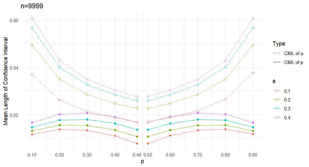
Figure 1: Symmetry in Mean Lengths of Confidence Intervals for ‘p’ about $p=0.5$

5.2 Test for independence

Tables 5 and 6 below present the results of the likelihood ratio test for independence in the Markov chain generated by copula model (2.1) and Bernoulli($p$) marginal distribution. The tables provide separate results for $p<1/2$ and $p>1/2$, respectively.

The Markov chain is generated using true values of $a$ and $p$, and subsequently, a chi-squared independence test is performed based on the test statistics $-2\log\Lambda_{1}$ and $-2\log\Lambda_{2}$, where $\Lambda_{1}$ and $\Lambda_{2}$ are given by formulae (4.3) and (4.4) respectively. A significance level of $\alpha=0.05$ is chosen for the test, implying that the null hypothesis of independence will be rejected if $-2\log\Lambda_{i}\geq 3.842,i=1,2$. Conversely, if $-2\log\Lambda_{i}<3.842$, the null hypothesis of independence is not rejected.

The chain is simulated for a total of $n+1$ steps, where $n$ is set to $9999$. The iterative process for Table 5 has values of $a$ (ranging from $0.1$ to $0.9$ with a step of $0.1$) and $p<1/2$ (ranging from $0.1$ to $0.4$ with a step of $0.1$). On the other hand, Table 6 had values of $a$ (ranging from $0.1$ to $0.9$ with a step of $0.1$) and $p>1/2$ (ranging from $0.6$ to $0.9$ with a step of $0.1$).

Table 5: Likelihood Ratio Test Results for the model based on copula (2.1) and Bernoulli ($p$) marginal distribution ($p<\frac{1}{2}$)

a	p	$-2\log\Lambda_{1}$	Decision on $H_{0}$
0.1	0.1	1.9648	Do not reject
0.1	0.2	75.3318	Reject
0.1	0.3	465.3507	Reject
0.1	0.4	1302.2148	Reject
0.2	0.1	62.5624	Reject
0.2	0.2	0.5426	Do not reject
0.2	0.3	91.6928	Reject
0.2	0.4	537.1743	Reject
0.3	0.1	178.0430	Reject
0.3	0.2	85.5790	Reject
0.3	0.3	-0.6683	Do not reject
0.3	0.4	143.3914	Reject
0.4	0.1	315.6163	Reject
0.4	0.2	282.6401	Reject
0.4	0.3	93.5413	Reject
0.4	0.4	-0.7403	Do not reject
0.5	0.1	598.6498	Reject
0.5	0.2	678.1999	Reject
0.5	0.3	443.8051	Reject
0.5	0.4	175.6443	Reject
0.6	0.1	986.4705	Reject
0.6	0.2	1060.7808	Reject
0.6	0.3	908.5222	Reject
0.6	0.4	520.2437	Reject
0.7	0.1	1243.0918	Reject
0.7	0.2	1596.5124	Reject
0.7	0.3	1581.8311	Reject
0.7	0.4	1243.7897	Reject
0.8	0.1	1548.5890	Reject
0.8	0.2	2291.3934	Reject
0.8	0.3	2551.6879	Reject
0.8	0.4	2361.9013	Reject
0.9	0.1	2466.6171	Reject
0.9	0.2	3305.7161	Reject
0.9	0.3	3631.3346	Reject
0.9	0.4	3835.4538	Reject

Table 6: Likelihood Ratio Test Results for the model based on copula (2.1) and Bernoulli ($p$) marginal distribution ($p\geq\frac{1}{2}$)

a	p	$-2\log\Lambda_{2}$	Decision on $H_{0}$
0.1	0.6	279.8288	Reject
0.1	0.7	107.8140	Reject
0.1	0.8	16.0485	Reject
0.1	0.9	0.3192	Fail to reject
0.2	0.6	111.3087	Reject
0.2	0.7	17.5196	Reject
0.2	0.8	0.4450	Fail to reject
0.2	0.9	12.1072	Reject
0.3	0.6	38.3697	Reject
0.3	0.7	-1.3511	Fail to reject
0.3	0.8	15.9764	Reject
0.3	0.9	26.5985	Reject
0.4	0.6	0.0341	Fail to reject
0.4	0.7	17.6239	Reject
0.4	0.8	50.2535	Reject
0.4	0.9	62.1340	Reject
0.5	0.6	16.9398	Reject
0.5	0.7	97.3027	Reject
0.5	0.8	127.9626	Reject
0.5	0.9	165.1340	Reject
0.6	0.6	118.6838	Reject
0.6	0.7	195.6122	Reject
0.6	0.8	209.1521	Reject
0.6	0.9	222.3218	Reject
0.7	0.6	279.7745	Reject
0.7	0.7	328.9172	Reject
0.7	0.8	315.8419	Reject
0.7	0.9	263.6996	Reject
0.8	0.6	522.4635	Reject
0.8	0.7	557.5287	Reject
0.8	0.8	533.2392	Reject
0.8	0.9	284.6627	Reject
0.9	0.6	768.7074	Reject
0.9	0.7	688.8740	Reject
0.9	0.8	545.8894	Reject
0.9	0.9	411.5155	Reject

The test indicates that when $a=p<1/2$ or $a=1-p\leq 1/2$, the Markov chain model generated by copula (2.1) and the Bernoulli($p$) marginal distribution transforms into independent Bernoulli trials.

5.3 Comparison of different estimators for the mean

This section is dedicated to the performance of the different estimators of the Bernoulli parameter. The MLEs are obtained numerically and their confidence intervals are constructed. The sample mean satisfies the central limit theorem (9). The $(1-\alpha)100\%$ confidence intervals for $p$ are therefore

$$\begin{cases}\bar{p}\pm z_{\alpha/2}\left[\frac{\bar{p}(1-\bar{p})}{n+1}\left(\frac{1+a-2\bar{p}}{1-a}\right)\right]^{1/2}&\quad\text{when}\ p<1/2\\ \bar{p}\pm z_{\alpha/2}\left[\frac{\bar{p}(1-\bar{p})}{n+1}\left(\frac{a+2\bar{p}-1}{1-a}\right)\right]^{1/2}&\quad\text{when}\ p\geq 1/2.\end{cases}$$

The other estimator for the mean ($p$) considered here is the robust estimator proposed by Longla and Peligrad (2021) [29]. It is based on a sample of dependent observations and requires some mild conditions to be satisfied on the variance of partial sums. The procedure is as follows: Given the sample data $(X_{t})_{0\leq t\leq n}$ from a stationary sequence $(X_{t})_{t\in\mathbb{Z}}$, we generate another random sample $(Y_{t})_{0\leq t\leq n}$ independently of $(X_{t})_{0\leq t\leq n}$ and following a standard normal distribution. The Gaussian kernel and the optimal bandwidth $h_{n}$ are used. Denoting by $\bar{X^{2}}_{n}$ the sample averages of $X^{2}$ and $\bar{p}$ the sample mean of $(X_{t})_{0\leq t\leq n}$, the optimal bandwidth, as proposed in Longla and Peligrad (2021) [29], for our case is

$$h_{n}=\left(\frac{1}{(n+1)\sqrt{2}}\right)^{1/5}.$$ (5.1)

To use this estimator, the following conditions must be satisfied (i.) $(X_{t})_{t\in\mathbb{Z}}$ is an ergodic sequence, (ii.) $(X_{t})_{t\in\mathbb{Z}}$ has finite second moments and (iii.) $(n+1)h_{n}var(\bar{p})\longrightarrow 0$ as $n\longrightarrow\infty.$ These conditions are easy to verify: ($i.$) The Markov chain $X$ is $\psi$-mixing, and hence ergodic. ($ii.$) The second condition follows from that $Var(X_{0})=p(1-p)<\infty\ \text{and}\ E[X_{0}]=p$. ($iii.$) Using the variance of $\bar{X}$ given by (3.18), we see that

$$(n+1)\left(\frac{1}{(n+1)\sqrt{2}}\right)^{1/5}\left[\frac{p(1-p)}{(n+1)}\left(\frac{1+a-2p}{1-a}\right)+O(1/n)\right]\longrightarrow 0$$

as  $n\longrightarrow\infty.$ The proposed robust estimator for the mean $(p)$ of $X$ is

$$\tilde{p}=\frac{1}{(n+1)h_{n}}\sum_{t=0}^{n}X_{t}\exp\left(-\frac{1}{2}\left(\frac{Y_{t}}{h_{n}}\right)^{2}\right).$$

A $(1-\alpha)100\%$ confidence interval for $p$ is

$$\tilde{p}\sqrt{1+h_{n}^{2}}\pm z_{\alpha/2}\left[\frac{\bar{Y}_{n}^{2}}{(n+1)\sqrt{2}h_{n}}\right]^{1/2}.$$

Tables 7 and 8 below present a comparison of the three estimators of $p$ across varying true values of $p$. Samples of size $n+1$ were utilized, and 95% confidence intervals were constructed. Coverage probabilities were computed based on $400$ replications of each of the chains of size $n+1$. Subsequently, the means of the lengths of the $400$ confidence intervals were calculated to determine the confidence interval mean length. The results in both tables demonstrate that the estimators are asymptotically equivalent and converge to the true value. Note that we did not include the numerical values of the estimators because $400$ numerical values were computed for each estimator in each case, and there is no criterion to choose only one representative from the $400$. Relatively narrow confidence intervals reflect a higher level of precision in estimation, while wider confidence intervals indicate greater uncertainty in estimation.

Table 7: A comparison of the performance of $\hat{p}$, $\bar{p}$ and $\tilde{p}$ for $p<0.5$. A fixed value of $a=0.5$ was used in all the cases and 95% confidence intervals were constructed.  Est denotes estimator and $p_{0}$ denotes the true value of $p$.

n		0.1	0.2	0.3	0.4
99	$\hat{p}$	CIML: 0.1862 CP: 0.8625	CIML: 0.2258 CP: 0.9100	CIML: 0.2355 CP: 0.9275	CIML: 0.2245 CP: 0.9400
	$\bar{p}$	CIML: 0.1896 CP: 0.9625	CIML:0.0.2325 CP: 0.9475	CIML: 0.2410 CP: 0.9575	CIML: 0.2272 CP: 0.9625
	$\tilde{p}$	CIML: 0.1656 CP: 0.7875	CIML: 0.2399 CP: 0.9000	CIML: 0.2946 CP: 0.9325	CIML: 0.3416 CP: 0.9500
499	$\hat{p}$	CIML: 0.0828 CP: 0.9050	CIML: 0.1030 CP: 0.9150	CIML: 0.1074 CP: 0.9450	CIML:0.1012 CP: 0.9300
	$\bar{p}$	CIML: 0.0848 CP: 0.9450	CIML: 0.1040 CP: 0.9550	CIML: 0.1078 CP: 0.9375	CIML:0.1016 CP: 0.9275
	$\tilde{p}$	CIML: 0.0889 CP: 0.8825	CIML: 0.1264 CP: 0.9325	CIML: 0.1550 CP: 0.9250	CIML: 0.1797 CP: 0.9675
999	$\hat{p}$	CIML: 0.0591 CP: 0.9375	CIML: 0.0732 CP: 0.9400	CIML: 0.0761 CP: 0.9375	CIML: 0.0717 CP: 0.9475
	$\bar{p}$	CIML: 0.0600 CP: 0.9375	CIML: 0.0735 CP: 0.9700	CIML: 0.0762 CP: 0.9575	CIML: 0.0719 CP: 0.9550
	$\tilde{p}$	CIML: 0.0678 CP: 0.8825	CIML: 0.0962 CP: 0.9200	CIML: 0.1179 CP: 0.9300	CIML: 0.1362 CP: 0.9550
4999	$\hat{p}$	CIML: 0.0267 CP: 0.9425	CIML: 0.0328 CP: 0.9575	CIML: 0.0341 CP: 0.9475	CIML: 0.0321 CP: 0.9350
	$\bar{p}$	CIML: 0.0268 CP: 0.9625	CIML: 0.0329 CP: 0.9600	CIML: 0.0341 CP: 0.9400	CIML: 0.0321 CP: 0.9525
	$\tilde{p}$	CIML:0.0356 CP: 0.9000	CIML: 0.0505 CP: 0.9200	CIML: 0.0619 CP: 0.9425	CIML: 0.0716 CP: 0.9450
9999	$\hat{p}$	CIML: 0.0189 CP: 0.9525	CIML: 0.0232 CP: 0.9550	CIML: 0.0241 CP: 0.9500	CIML: 0.0227 CP: 0.9300
	$\bar{p}$	CIML: 0.0190 CP: 0.9500	CIML: 0.0232 CP: 0.9570	CIML: 0.0241 CP: 0.9625	CIML: 0.0227 CP: 0.9450
	$\tilde{p}$	CIML: 0.0270 CP: 0.9025	CIML: 0.0383 CP: 0.9000	CIML: 0.0470 CP: 0.9500	CIML: 0.0542 CP: 0.9500

Table 8: A comparison of the performance of $\hat{p}$, $\bar{p}$ and $\tilde{p}$ for $p\geq 0.5$. A fixed value $a=0.5$ was used in all the cases and 95% confidence intervals were constructed.  Est denotes estimator and $p_{0}$ denotes the true value of $p$.

n		0.6	0.7	0.8	0.9
99	$\hat{p}$	CIML: 0.2242 CP: 0.9575	CIML: 0.2381 CP: 0.9275	CIML: 0.2286 CP: 0.9250	CIML: 0.1912 CP: 0.8900
	$\bar{p}$	CIML: 0.2272 CP: 0.9450	CIML: 0.2410 CP: 0.9575	CIML: 0.2326 CP: 0.9450	CIML: 0.1896 CP: 0.9500
	$\tilde{p}$	CIML: 0.4163 CP: 0.9450	CIML: 0.4529 CP: 0.9525	CIML: 0.4841 CP: 0.9575	CIML: 0.5124 CP: 0.9700
499	$\hat{p}$	CIML: 0.1013 CP: 0.9200	CIML: 0.1071 CP: 0.9425	CIML: 0.1032 CP: 0.9550	CIML: 0.0832 CP: 0.9075
	$\bar{p}$	CIML: 0.1016 CP: 0.9575	CIML: 0.1077 CP: 0.9475	CIML: 0.1040 CP: 0.9475	CIML: 0.0848 CP: 0.9400
	$\tilde{p}$	CIML: 0.2200 CP: 0.9450	CIML: 0.2381 CP: 0.9650	CIML: 0.2543 CP: 0.9500	CIML: 0.2695 CP: 0.9775
999	$\hat{p}$	CIML: 0.0716 CP: 0.9275	CIML: 0.0759 CP: 0.9175	CIML: 0.0731 CP: 0.9400	CIML: 0.0595 CP: 0.9225
	$\bar{p}$	CIML: 0.0719 CP: 0.9475	CIML: 0.0762 CP: 0.9350	CIML: 0.0735 CP: 0.9625	CIML: 0.0600 CP: 0.9175
	$\tilde{p}$	CIML: 0.1664 CP: 0.9525	CIML: 0.1803 CP: 0.9725	CIML: 0.1926 CP: 0.9550	CIML: 0.2042 CP: 0.9375
4999	$\hat{p}$	CIML: 0.0321 CP: 0.9400	CIML: 0.0341 CP: 0.9425	CIML: 0.0329 CP: 0.9500	CIML: 0.0268 CP: 0.9400
	$\bar{p}$	CIML: 0.0321 CP: 0.9550	CIML: 0.0341 CP: 0.9275	CIML: 0.0329 CP: 0.9525	CIML: 0.0268 CP: 0.9625
	$\tilde{p}$	CIML: 0.0876 CP: 0.9475	CIML: 0.0946 CP: 0.9525	CIML: 0.1012 CP: 0.9500	CIML: 0.1073 CP: 0.9525
9999	$\hat{p}$	CIML: 0.0227 CP: 0.9500	CIML: 0.0241 CP: 0.9500	CIML: 0.0233 CP: 0.9475	CIML: 0.0190 CP: 0.9425
	$\bar{p}$	CIML: 0.0227 CP: 0.9500	CIML: 0.0241 CP: 0.9450	CIML: 0.0233 CP: 0.9450	CIML: 0.0190 CP: 0.9500
	$\tilde{p}$	CIML: 0.0664 CP: 0.9700	CIML: 0.0717 CP: 0.9725	CIML: 0.0767 CP: 0.9700	CIML: 0.0813 CP: 0.9650

In both cases of $p<1/2$ and $p>1/2$, $\hat{p}$ yields the most precise estimates with the shortest mean confidence intervals. The sample mean closely follows $\hat{p}$ in precision but exhibits slightly longer mean confidence intervals. Although the robust estimator shows larger mean confidence intervals compared to $\hat{p}$ and $\bar{p}$, it still provides reasonable estimates, especially with larger sample sizes. This comparison is presented on the plots in Figure 2 and Figure 3.

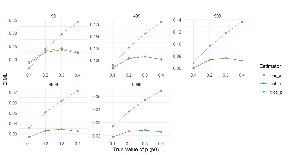
Figure 2: Confidence Interval Mean Lengths (CIML) for different estimators of $p<\frac{1}{2}$

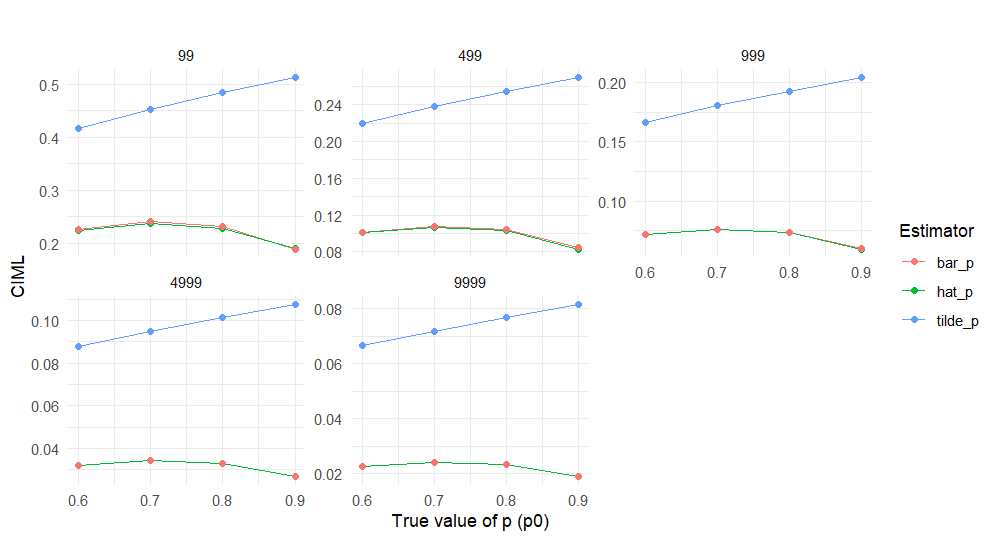
Figure 3: Confidence Interval Mean Lengths (CIML) for different estimators of p>1/2

Both the MLE and the robust estimator demonstrate sensitivity to sample size, resulting in initially low coverage probabilities. However, as the sample size increases, these probabilities approach the desired 95% level. The coverage probabilities for the sample mean $(\bar{p})$ consistently approach the desired nominal level, indicating reliable confidence intervals across different sample sizes.

The performance of the robust estimator is less optimal with smaller sample sizes but improves as the sample size increases. The robust estimator is designed to be competitive in data containing noise or outliers; however, the data considered here has neither.

While all three estimators provide estimates for the Bernoulli parameter $p$, the MLE ($\hat{p}$) generally strikes the best balance between precision and accuracy, making it the preferred choice for estimating $p$ in this context.

6 Conclusion

The mixing properties of copula-based Markov chains are highly dependent on the chosen marginal distributions. Some copulas that do not generate mixing with continuous marginals may generate mixing with discrete marginals, so generalizations should be approached with caution. In this paper, we have demonstrated that copulas from the Fréchet (Mardia) family generate $\psi$-mixing Markov chains for $a+b=1$, which is not the case when the marginals are uniform$[0,1]$. Understanding these mixing properties is crucial for deriving central limit theorems for sample means, which in turn facilitates the construction of confidence intervals for the sample means based on the standard normal distribution.

References

- [1] Charles A Johnson and Jerome H Klotz. The atom probe and markov chain statistics of clustering. Technometrics, 16(4):483–493, 1974.
- [2] Edwin L Crow. Approximate confidence intervals for a proportion from markov dependent trials. Communications in Statistics-Simulation and Computation, 8(1):1–24, 1979.
- [3] Barron Brainerd and Sun Man Chang. Number of occurrences in two-state markov chains, with an application in linguistics. The Canadian Journal of Statistics/La revue canadienne de statistique, pages 225–231, 1982.
- [4] FN David. A power function for tests of randomness in a sequence of alternatives. Biometrika, 34(3/4):335–339, 1947.
- [5] Leo A Goodman. Simplified runs tests and likelihood ratio tests for markoff chains. Biometrika, 45(1/2):181–197, 1958.
- [6] Theodore W Anderson and Leo A Goodman. Statistical inference about markov chains. The annals of mathematical statistics, pages 89–110, 1957.
- [7] Patrick Billingsley. Statistical inference for Markov processes, volume 2. University of Chicago Press, Chicago, 1961.
- [8] Martial Longla. On mixtures of copulas and mixing coefficients. Journal of Multivariate analysis, 139:259–265, 2015.
- [9] Roger B Nelsen. Methods of constructing copulas. An introduction to copulas, pages 51–108, 2006.
- [10] William F Darsow, Bao Nguyen, and Elwood T Olsen. Copulas and markov processes. Illinois journal of mathematics, 36(4):600–642, 1992.
- [11] Patrick Billingsley. Statistical methods in markov chains. The annals of mathematical statistics, pages 12–40, 1961.
- [12] Jerome Klotz. Markov chain clustering of births by sex. In Proc. Sixth Berkeley Symp. Math. Statist. Prob, volume 4, pages 173–185, 1972.
- [13] Jerome Klotz. Statistical inference in bernoulli trials with dependence. The Annals of statistics, pages 373–379, 1973.
- [14] Bertram Price. A note on estimation in bernoulli trials with dependence. Communications in Statistics-Theory and Methods, 5(7):661–671, 1976.
- [15] Bo Lindqvist. A note on bernoulli trials with dependence. Scandinavian Journal of Statistics, pages 205–208, 1978.
- [16] Harry Joe. Multivariate models and multivariate dependence concepts. CRC press, Boca Raton, Fla., 1997.
- [17] Fabrizio Durante and Carlo Sempi. Principles of copula theory. CRC press, Boca Raton, Fla., 2015.
- [18] Martial Longla. On dependence structure of copula-based markov chains. ESAIM: Probability and Statistics, 18:570–583, 2014.
- [19] M Sklar. Fonctions de repartition an dimensions et leurs marges. Publ. inst. statist. univ. Paris, 8:229–231, 1959.
- [20] Martial Longla and Magda Peligrad. Some aspects of modeling dependence in copula-based markov chains. Journal of Multivariate Analysis, 111:234–240, 2012.
- [21] IA Ibragimov. Some limit theorems for stochastic processes stationary in the strict sense. In Dokl. Akad. Nauk SSSR, volume 125, pages 711–714, 1959.
- [22] Robert Cogburn. Asymptotic properties of stationary sequences, volume 3. University of California Press, Oakland, CA, 1960.
- [23] JR Blum, David Lee Hanson, and Lambert Herman Koopmans. On the strong law of large numbers for a class of stochastic processes. Sandia Corporation, Albuquerque, NM, 1963.
- [24] Walter Philipp. The central limit problem for mixing sequences of random variables. Zeitschrift für Wahrscheinlichkeitstheorie und verwandte Gebiete, 12(2):155–171, 1969.
- [25] Richard C Bradley. Introduction to strong mixing conditions. (No Title), 2007.
- [26] Edward J Bedrick and Jorge Aragon. Approximate confidence intervals for the parameters of a stationary binary markov chain. Technometrics, 31(4):437–448, 1989.
- [27] I Ibragimov. Independent and stationary sequences of random variables. Wolters, Noordhoff Pub., 1975.
- [28] Samuel S Wilks. The large-sample distribution of the likelihood ratio for testing composite hypotheses. The annals of mathematical statistics, 9(1):60–62, 1938.
- [29] Martial Longla and Magda Peligrad. New robust confidence intervals for the mean under dependence. Journal of Statistical Planning and Inference, 211:90–106, 2021.