The defect energy formalism for CALPHAD thermodynamics of dilute point defects: Theory

Abstract

The thermodynamics of point defects is crucial for determining the functional properties of various materials. Typically, defect stability is assessed using grand-canonical defect formation energy, which requires deducing the equilibrium chemical potential or Fermi level that governs atom and electron exchange with the environment. This process is complicated by the interplay of chemical potential and Fermi level and their dependence on composition and temperature. Typically, the grand-canonical formation energy is incorporated as an additional term to the bulk Gibbs energy, creating a defect-centric framework where each new defect state necessitates a distinct Gibbs energy formulation. The calculation of phase diagrams (CALPHAD) method offers a more flexible alternative by integrating defect energies into the total Gibbs energy model, allowing for easier extrapolation to more complex compositions. Additionally, CALPHAD unifies the analysis of chemically and electronically driven defects using chemical composition as the primary variable. However, the Compound Energy Formalism (CEF) used in CALPHAD has limitations, including a lack of clear connections between defect formation energies and Gibbs energy parameters and an exponential increase in complexity with added chemical or charge variations. We present the theoretical derivation of the Defect Energy Formalism (DEF), which we have recently proposed. DEF overcomes the limitations of CEF by establishing explicit relationships between the absolute defect energies—independent of chemical potential or Fermi level—and the Gibbs energy parameters of defective compounds. This results in a first-principles model for dilute defects, eliminating the need for model fitting to experimental or simulation data. Additionally, DEF reduces the inherent complexity of CEF by applying the superposition of absolute defect energies, making it feasible for modeling multi-component and chemically complex compounds. This paper presents a formal, general derivation of DEF and offers guidelines for its application, promising more accurate and efficient thermodynamic modeling of defective materials.

I Introduction

Thermodynamics of point defects determines the functional properties of many materials in several applications, from semiconductors (thermoelectrics Pei et al. (2011); Jood et al. (2020); Seebauer and Kratzer (2006); Zheng et al. (2021); Slade et al. (2021); Jiang et al. (2014), photovoltaics Ganose et al. (2022); Huang et al. (2018); Park et al. (2018); Vidal et al. (2012); Geisz and Friedman (2002); Tongay et al. (2013); Mora-Seró (2020); Park and Walsh (2019); Walsh and Zunger (2017)) to insulators (optical materials G. Pacchioni (85 0); Raghavachari et al. (2002); Mills (1980); Ma and Rohlfing (2008); Girard et al. (2019); Bourrellier et al. (2016); Tuller and Bishop (2011); Brecher et al. (1990), ion-conducting materials Tuller and Bishop (2011); Tuller (2003); Aidhy et al. (2015); Zhang et al. (2020); Li et al. (2019); Defferriere et al. (2021), non-stoichiometric materials Defferriere et al. (2021); Li et al. (2020); Marrocchelli et al. (2012); Noureldine et al. (2015); Boehm et al. (2005)). The thermodynamics of isolated defects in solids is well-established through formation energies, typically defined as the excess grand-potential energy in a grand-canonical ensemble, offering a defect-centric perspective Rogal et al. (2014); Anand et al. (2022); Toriyama et al. (2022). First principles methods like density functional theory (DFT) have significantly advanced, enabling precise calculations of formation energies for various point defects (vacancies, interstitials, antisites) across different charge states Freysoldt et al. (2014); Hine et al. (2009); Ramprasad et al. (2012); Lany and Zunger (2008, 2010, 2009). In this defect-centric approach, the defect formation free energy is considered an additional contribution to the total free energy, expressed as ($G=G(\text{bulk})+\Delta G_{\text{defect}}$). However, this method is inherently system-specific, requiring the determination of a new $\Delta G_{\text{defect}}$ term for each new composition or higher-order multi-component system. The CALPHAD approach offers an adaptable alternative by incorporating the influence of defects directly into the comprehensive description of total free energy rather than treating them as isolated excess terms. In this framework, defects are introduced as distinct entities that interact with other components, such as chemical elements. Their impact on the Gibbs energy is integrated into interaction parameters within the CALPHAD model. CALPHAD’s hierarchical formulation enables straightforward extrapolation to higher-order multi-component systems. For instance, interaction parameters initially determined for a binary compound can be leveraged to predict free energy across other compositions, including ternary compounds.

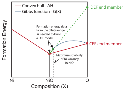
Figure 1: Linear Mapping Principle underlying DEF. Comparing CEF and DEF for thermodynamic modeling of dilute Ni vacancies in Ni_1-$\delta$O. The schematic Gibbs energy is given by the blue curve, approximated in CALPHAD using interpolation of end-member parameters. Traditional CEF uses the fully defective end-member, which in this case is O, and effectively approximates the blue curve with the red line, which greatly underestimates the $G$ of NiO with dilute Ni vacancies. The DEF method, in contrast, approximates the blue curve with the green line derived from the slope as it approaches the pristine compound (‘dilute limit’). The DEF provides a much more accurate estimate of $G$ in the composition region pertinent to dilute defect concentrations.

The CALPHAD method for collecting, reporting, and computing thermodynamic data has been hugely successful both in industry and academia, leading to the rapid development of metal alloys for numerous applications Kattner (2016, 1997); Hickel et al. (2014); Campbell et al. (2014); Liu and Wang (2016); Sundman et al. (2018); van de Walle et al. (2017); Liu (2009); Bajaj et al. (2011); Li et al. (2021); van de Walle (2013); van de Walle et al. (2018). For ordered ionic compounds and semiconductors, the compound energy formalism (CEF) has often been utilized Hillert and Staffansson (1970); Harvig et al. (1971); Sundman and Ågren (1981); Andersson et al. (1986); Hillert (2001); Frisk and Selleby (2001), which divides the lattice into different sublattices. Each sublattice can host various constituents (e.g., chemical element or vacancy). An “end member” represents a specific combination of these constituents on the sublattices, where each constituent exclusively occupies one sublattice. CEF formulates the Gibbs energy using these end members as the primary first-order parameters, while higher-order parameters characterize interactions among constituents within individual sublattices Hillert (2001). Defective compounds (e.g., non-stoichiometric oxides) can be recognized in CEF by defining point defects as constituents on the relevant sublattice. For example, non-stoichiometry of Ni_1-$\delta$O can be defined as (Ni,Vac)(O) (see Figure 1).

We have identified two bottlenecks in CEF that limit its application in describing defective compounds. Firstly, there lacks a clear connection between defect formation energies and the CEF parameters of Gibbs energy. While previous studies Hillert (2001); Rogal et al. (2014); Oates et al. (1995); Chen et al. (1998); Li and Kerr (2013) have hinted at connections between defect formation energies and Gibbs energies of end members, a systematic relationship remains elusive. Consequently, most studies use a standard “assessment” approach, fitting parameters to available experimental and computational data. This approach limits model development to specific material and thermodynamic ranges (temperatures, compositions) where data is accessible, hindering the creation of first-principles models. Even studies using first-principles DFT to compute defect formation energies typically use these values merely as starting points for fitting assessments to experimental data Hu et al. (2018); Peters et al. (2019, 2017); Bajaj et al. (2015); Li and Kerr (2013), rather than as direct inputs into Gibbs energy formulation. Secondly, the number of parameters in the CEF Gibbs energy formulation grows exponentially with added chemical or charge complexity (e.g., doped impurities, alloying components, or charged defects). CEF includes all potential end members as independent parameters, making it excessively intricate for multi-component and chemically complex compounds, as well as for describing charge carriers such as holes and free electrons. This computational complexity has constrained existing models of defective semiconductors and insulators to a limited set of binary examples where experimental data exists, so the model can ultimately be fit to experimental data (e.g., GaAs Chen and Hillert (1996), CdTe Chen et al. (1998), UO2 Sundman et al. (2011), PbSe Peters et al. (2019), PbX (X=S,Te) Peters et al. (2017); Bajaj et al. (2015), ZnS Guan et al. (2017), ZnO Li and Kerr (2013)).

To address the existing limitations of CEF, we theoretically derive the Defect Energy Formalism (DEF) as a special case of CEF for CALPHAD thermodynamics of dilute defects. For formulating the Gibbs energy of a defective compound, DEF applies two main principles pertinent to dilute defects:

First is the linear mapping of defect formation energies along chemical composition, inspired by an earlier study by Anand et al Anand et al. (2021), showing that the projection of a defective compound energy to its constituent species on the convex hull reflects the defect formation energy. Here, we evolve this concept to establish the physics-based relationship between DEF end members and defect formation energies. Additionally, we show that the Boltzmann statistics of dilute charge carriers naturally arise in the DEF formalism, similar to the CEF formalism. Figure 1 illustrates the concept of defining DEF end-members from the projection of the defect formation energy on the convex hull to its constituent species. This concept underlies the principle of linear mapping, as implemented in DEF and detailed in this work.

Second is applying the superposition principle to the Gibbs energy of DEF end-members containing multiple defects, offering a computationally efficient framework by reducing the number of independent end-members in the sublattice model. In a system with $s$ sublattices, each hosting $N_{s}$ constituents, the number of CEF end-members equals $\prod_{s}N_{s}$, whereas for DEF it equals $\sum_{s}N_{s}$. In simpler terms, DEF simplifies the complexity of CEF parameters from a combinatorial factor of single-defect end-members to a summation. This reduction stems naturally from the superposition principles applicable to dilute defects, unlike CEF, which handles arbitrary constituent mixing on each sublattice. A DEF end-member with multiple defects describes a compound hosting non-interacting, isolated defects, unlike CEF, where an end-member with multiple defects corresponds to “fictitious” end members with unrealistically high concentrations of interacting defects (see Figure 1).

In a recent study, we introduced DEF and demonstrated its application, confirming its feasibility Adekoya and Snyder (2024). Here, we present a formal derivation of the DEF applicable to any type of point defects (vacancies, interstitials, and anti-sites), offering guidelines for constructing DEF models for any materials and combinations of dilute point defects. The organization of this paper is as follows: In section II, we derive the DEF formulation for defective compounds with neutral defects, detailing the derivation of DEF end-member Gibbs energy in section II.1 and the construction of DEF sublattice models in sections II.2 and II.3. In section III, we derive the DEF formulation for defective compounds with charged defects, followed by constructing a DEF sublattice model in section III.1. Section IV presents general guidelines for constructing DEF for any compounds and combinations of defects.

II Defect Energy Formalism for Neutral Defects

The DEF construct is a modified version of the standard CEF, seen as a special case with specific constraints on the mixing behavior of its constituents. A phase in DEF is divided into one, two or more sublattices, labeled $s$, each containing $N_{s}$ constituents. For instance, (A,C)_p(B,D,E)_q represents a typical two-sublattice model where A and C mix on the first sublattice and B, D, and E mix on the second, with $p$ and $q$ as stoichiometric coefficients for a formula unit containing $p+q$ atoms. In a typical CEF model, each sublattice can mix multiple primary constituents at arbitrary ranges. In DEF, however, defect concentrations remain in the dilute range, so defects are considered secondary constituents. Here, we focus on DEF models where each sublattice hosts one primary constituent (an atomic species) and multiple defects (e.g., vacancies, anti-sites, or interstitials) as secondary constituents, such as (A,Vac,B)_p(B,A)_q for A-vacancy and B-antisite, and A-antisite. End-members represent phases with only one constituent per sublattice. Within the DEF construct, one end-member corresponds to defect-free ordered compounds with each sublattice hosting primary constituents (e.g., (A)_p(B)_q), while others are defective compounds with at least one defect constituent on a sublattice (e.g., (Vac)_p(B)_q). Despite appearing as nonphysical due to the notation showing high defect concentrations (e.g., (Vac)_p(B)_q), defective end-members in DEF actually correspond to physical compounds with dilute defect concentrations (see Figure 1).

The constitution of a DEF phase is described by the site fractions of each constituent $J$ on each sublattice $s$, denoted by $y^{s}_{J}$. The summation of constituents’ site fractions on each sublattice yields 1, or $\sum_{J}y^{s}_{J}=1$. The content of each component $I$ per formula unit is then related to the site fractions on individual sublattices according to the following equation (see equation 4 in Ref. Hillert (2001)):

$$X_{I}=\frac{\sum_{s}{a^{s}y^{s}_{I}}}{\sum_{s}{a^{s}\left(1-y^{s}_{\text{vac}}\right)}}$$ (1)

where $a^{s}$ is the stoichiometry coefficient of sublattice $s$. The composition $X\textsubscript{I}$ denotes the composition of a component per formula unit of atoms and not per site. Therefore, it directly relates to the composition space in a typical convex hull or phase diagram. We refer to the composition space as the $X$-space and the constitution of DEF site fractions as the $Y$-space.

The Gibbs energy per formula unit of the DEF phase, $G_{\text{uf}}$, is defined by the surface of reference energy $G_{\text{uf}}^{\text{s.r.}}$ along with the ideal mixing entropy, following the CEF (see equations 1 and 2 in Ref.Hillert (2001)). Here, $G_{\text{uf}}^{\text{s.r.}}$ is a linear interpolation of end-member Gibbs energies, ${}^{0}G_{\text{end}}$, as follows:

$$\begin{split}&G_{\text{fu}}=G_{\text{fu}}^{\text{s.r.}}+kT\sum_{s}\sum_{J}a^{s}y^{s}_{J}\ln(y^{s}_{J})\\ &G_{\text{fu}}^{\text{s.r.}}=\sum_{\text{end-members}}{{}^{0}G_{\text{end}}\prod_{s}y^{s}_{J}}\end{split}$$ (2)

where $k$ and $T$ denote the Boltzmann constant and temperature, respectively. In the $G_{\text{uf}}^{\text{s.r.}}$ formula, the summation runs over all end members, and the product runs over all sublattices in the DEF model. For each end-member, $J$ consists only of the constituents corresponding to that end-member. In DEF, we do not include the excess Gibbs energy term, commonly denoted as ${}^{E}G$ in a typical CEF model. This is because at dilute defect concentrations, the primary constituent and secondary defects mix like an ideal solution, where each added defect reduces the number of solvent atoms, making chemical activity proportional to chemical composition (i.e., Raoult’s law for dilute solutions). Therefore, the only parameters of the Gibbs energy are the end-members, ${}^{0}G_{\text{end}}$.

The grand canonical formation energy for a neutral defect is defined as

$$\Delta H_{\text{d}}=E_{\text{def}}-E_{\text{pristine}}-\sum_{i}\Delta N_{i}\mu_{i}$$ (3)

where $E_{\text{def}}$ and $E_{\text{pristine}}$ denote the energies of the defective and pristine structures, respectively, $\Delta N_{i}$ is the number of atoms of species $i$ added to or removed from the defective structure (e.g., +1 for interstitials, -1 for vacancies) and $\mu_{i}$ is the chemical potential of the species $i$. The defect formation energy depends on the chemical equilibrium condition through the last term, which measures the chemical work associated with the exchange of an atomic species between the host compound and the chemical reservoir. The chemical potential of species $i$ is equal in both the host compound and the chemical reservoir, as dictated by the condition of chemical equilibrium.

We relate the grand-canonical formation energy from equation 3 to the DEF end-member Gibbs energy, ${}^{0}G_{\text{end}}$, from equation 2, inspired by Anand et al.’s graphical representation of defect formation energy on the convex hull Anand et al. (2021). They showed that projecting the defective compound formation energy relative to the (extended) convex hull onto its constituent species gives the defect formation energy of equation 3. Their derivation applies to any chemical equilibrium condition, such as the coexistence of defective A_pB_qwith A-vacancy and pure A. In the CALPHAD framework, equilibrium is determined by common tangents on the convex hull. Therefore, the chemical potential of A-vacancy formation in a binary A_pB_qcompound (without other defects) is derived from the B-rich condition, indicated by the common tangent at the defective compound’s composition. In section II.1, we show that when the absolute defect energy is projected onto the convex hull’s relevant endpoint and adjusted to a unified reference energy, it becomes independent of the chemical potential. This energy, independent of chemical potential, directly relates to the DEF end-member Gibbs energy. In sections II.2 and II.3, we demonstrate the construction of DEF for various defective compounds with neutral point defects.

II.1 From defect formation energies on the convex hull to DEF end-member

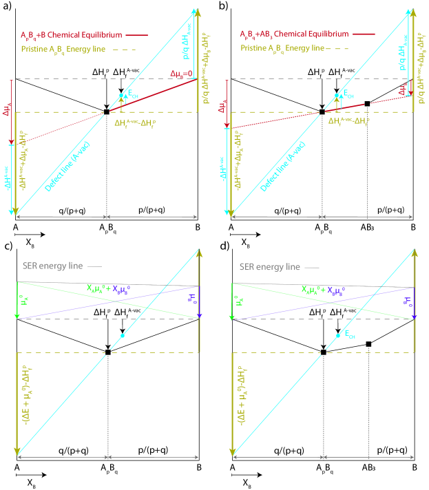
Figure 2: Formation energy per atom convex hull. a,b) Graphical representation of an A-vacancy formation energy and chemical potential change for model (a)A-A_pB_q-B and (b) A-A_pB_q-AB3-B convex hulls. The equilibrium chemical condition is determined by the common tangent line at the defective compound composition, A_pB_q+B coexistence line for (a) and A_pB_q+AB3 coexistence line for (b). The formation energy of the defect-free A_pB_qand defective A_pB_qare shown by the black square and blue circle, respectively. $E_{\text{CH}}$ denotes the convex-hull distance, defined as the distance of the defective structure above the convex hull (see Ref.Anand et al. (2021)). The common tangent lines determining the chemical potential condition are shown by bold red lines. Defect lines connecting the defective and pristine formation energies are shown by blue lines. The projection of $E_{\text{CH}}$ and common tangent line onto the A-end give the grand-canonical defect formation energy and chemical potential of A, respectively. The absolute defect energy, $\Delta H^{\text{d}}_{\text{f}}-\Delta H^{\text{p}}_{\text{f}}$, and its projections on the A-end and B-end are shown by yellow arrows. c,d) Graphical representation of adjusting the projected absolute defect energies to the common SER reference line for (c) A-A_pB_q-B and (d) A-A_pB_q-AB3-B convex hulls. The projected absolute energies and the adjustment energies are all independent of the convex hull shape and, therefore, the equilibrium chemical conditions determined by it.

In this section, we convert the defect formation energy, projected onto the convex hull endpoint, to the DEF Gibbs energy of defective end members. Anand et al. illustrated how to obtain the grand-canonical defect formation energy, $\Delta H_{\text{d}}$ from equation 3, by projecting the defective structure’s formation energy distance relative to the (extended) convex hull onto the relevant endpoint Anand et al. (2021)(see Figure 2(a) and (b)). Here, instead of a general chemical equilibrium condition, we impose the chemical equilibrium condition from the convex hull’s common tangent so that no extended convex hull is considered. Also, we project the absolute defect energy instead of the convex hull distance and unify all energies, including formation energies of defective and pristine compounds and the absolute defect energy using a common reference energy. This unification is crucial for mapping defect formation energies onto DEF end members, showing that the DEF defective end-member Gibbs energy is directly related to a chemical-potential-independent absolute defect energy.

Considering A_pB_qwith p + q atoms in its primitive cell, the formation energies of the pristine and defective compounds ($\Delta H^{\text{p}}_{\text{f}}$ and $\Delta H^{\text{d}}_{\text{f}}$) are defined with reference to their pure states. We reformulate the defect formation energy of equation 3 in terms of $\Delta H^{\text{p}}_{\text{f}}$ and $\Delta H^{\text{d}}_{\text{f}}$. If the total energies of the defective ($E_{\text{def}}$) and pristine ($E_{\text{pristine}}$) structures are calculated for a supercell with $l$ times more atoms than the primitive cell , the formation energies (per atom) of the defective and pristine structures are defined as

$$\begin{split}\Delta H^{\text{d}}_{\text{f}}&=\frac{E_{\text{def}}-lp\mu^{0}_{A}-lq\mu^{0}_{B}-\sum\Delta N_{i}\mu^{0}_{i}}{l(p+q)+\sum\Delta N_{i}}\\ \Delta H^{\text{p}}_{\text{f}}&=\frac{E_{\text{pristine}}-lp\mu^{0}_{A}-lq\mu^{0}_{B}}{l(p+q)}\\ \end{split}$$ (4)

where $\mu^{0}_{A}$ and $\mu^{0}_{B}$ are the chemical potential (reference energy) of elements A and B in their standard state. $\mu^{0}_{i}$ is the reference chemical potential of species $i$ added or removed to form the defect, for example, A for an A interstitial in A_pB_q. Rewriting the defect formation energy of equation 3 in terms of the formation energies of the defective and pristine structures yields the following equation:

$$\begin{split}\Delta H_{\text{d}}&=\left(E_{\text{def}}-\sum_{i}\Delta N_{i}\mu_{i}\right)-E_{\text{pristine}}\\ =&\left(l(p+q)+\sum\Delta N_{i}\right)\left[\Delta H^{\text{d}}_{\text{f}}-\Delta H^{\text{p}}_{\text{f}}\right]\\ &+\sum\Delta N_{i}\Delta H^{\text{p}}_{\text{f}}-\sum\Delta N_{i}\Delta\mu_{i}\end{split}$$ (5)

Anand et al. used a different formulation of equation 5 (Eq. 10 in Ref. Anand et al. (2021)) to show that the projection of the convex hull distance of a defective compound, $E_{\text{CH}}$ in Figure 2, to the corresponding end on the convex hull ($i$ end) is equal to the defect formation energy $\Delta H_{\text{d}}$. This $\Delta H_{\text{d}}$ is chemical potential dependent. The equilibrium chemical potential is determined by the common tangent at the defective phase composition. As shown in Figure 2 (a) and (b) changes in the convex hull and the resulting common tangent affect both $\Delta H_{\text{d}}$ and $\Delta\mu_{i}$. However, DEF end-member Gibbs energies ${}{}^{0}G_{\text{end}}$ must be chemical-potential-independent and well-defined regardless of Gibbs energy changes in competing phases. Therefore, instead of projecting $E_{\text{CH}}$, which varies with the environment’s chemical potential, we project the chemical-potential independent value $\Delta H^{\text{d}}_{\text{f}}-\Delta H^{\text{p}}_{\text{f}}$, we call the absolute defect energy (see Figure 2 (a,b)). Note that $\Delta H^{\text{d}}_{\text{f}}-\Delta H^{\text{p}}_{\text{f}}$ measures the absolute defect energy of the defective compound relative to the pristine compound, setting the defect-free A_pB_qas the reference state, unlike $E_{\text{CH}}$, which measures the distance between the defective compound and the chemical potential energy line (convex hull common tangent). By rearranging equation 5, we project $\Delta H^{\text{d}}_{\text{f}}-\Delta H^{\text{p}}_{\text{f}}$ onto its corresponding endpoint as follows

$$\begin{split}&\Delta H_{\text{d}}+\sum\Delta N_{i}\Delta\mu_{i}-\sum\Delta N_{i}\Delta H^{\text{p}}_{\text{f}}\\ &=\overbrace{\left(l(p+q)+\sum\Delta N_{i}\right)}^{f_{i}^{d}}\left[\Delta H^{\text{d}}_{\text{f}}-\Delta H^{\text{p}}_{\text{f}}\right]\end{split}$$ (6)

As shown in Ref.Anand et al. (2021), $f_{i}^{d}$ is the projection factor that projects $E_{\text{CH}}$, and similarly $\Delta H^{\text{d}}_{\text{f}}-\Delta H^{\text{p}}_{\text{f}}$, to the $i$-end on the convex hull. Figure 2 illustrates this projection for a defective A_pB_qwith an A-vacancy. According to equation 6, the projection on the A-end is $-(\Delta H_{\text{A-vac}}-\Delta\mu_{A}+\Delta H^{\text{p}}_{\text{f}})$ with $\Delta N_{A}=-1$. The negative sign in front of the parenthesis arises from the A-vacancy projection factor, $f_{i}^{\text{\tiny A-vac}}$, which inverts the absolute defect energy direction when projected onto the opposite side relative to the A_pB_qcomposition (see Figure 2). As we elaborate later in section II.2, the A-vacancy defective compound corresponds to Vac:B DEF end-member and must be projected to the B-end. Accordingly, the B-end projection is $\frac{p}{q}(\Delta H_{\text{A-vac}}-\Delta\mu_{A}+\Delta H^{\text{p}}_{\text{f}})=\frac{p}{q}(\Delta H_{\text{A-vac}})+\Delta\mu_{B}-\Delta H^{\text{p}}_{\text{f}}$ (see Figure 2(a,b)). Note that $\Delta\mu_{A}$ and $\Delta\mu_{B}$ are related according to $\frac{p}{p+q}\Delta\mu_{A}+\frac{q}{p+q}\Delta\mu_{B}=\Delta H^{\text{p}}_{\text{f}}$. Although $\Delta H_{\text{d}}$ and $\sum\Delta N_{i}\Delta\mu_{i}$ (left hand side of equation 6) vary with chemical potential, their sum does not. Replacing $\Delta H_{\text{d}}$ from equation 3 into equation 6 results in $\Delta H_{\text{d}}+\sum\Delta N_{i}\Delta\mu_{i}=E_{\text{def}}-E_{\text{pristine}}-\sum\Delta N_{i}\mu_{i}^{0}=\Delta E_{\text{def}}-\sum\Delta N_{i}\mu_{i}^{0}$, a value that is independent of the chemical potential of the coexistence condition. $\Delta E_{\text{def}}$ is the difference between the total energy of the defective and pristine structures, commonly obtained through DFT total energy calculations. $\Delta E_{\text{def}}$ is chemical-potential-independent and needs to be calculated only once for a defective structure, regardless of its equilibrium conditions or coexistence with competing phases.

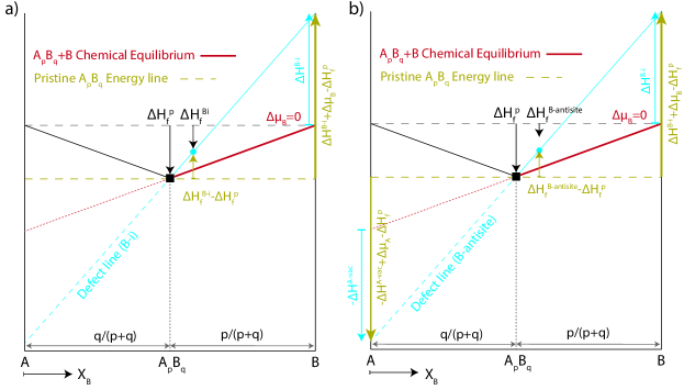
Figure 3: Formation energy per atom convex hull. Graphical representation of the absolute defect energy for a) B-interstitial and b) B-antisite in an A-A_pB_q-B convex hull.

Aside from projecting to the relevant end-point, we need to unify the reference energy between $\Delta H^{\text{p}}_{\text{f}}$, $\Delta H^{\text{d}}_{\text{f}}$, and the projection of equation 6. The reference state for $\Delta H^{\text{p}}_{\text{f}}$ and $\Delta H^{\text{d}}_{\text{f}}$ is the stable element reference (SER), as shown in Figure 2(c,d)) and equation 4. Accordingly, the projection of $\Delta H^{\text{d}}_{\text{f}}-\Delta H^{\text{p}}_{\text{f}}$ (equation 6), referenced to the pristine compound, must be adjusted to the SER. Additionally, we must convert the projection on the convex hull from per atom values to per formula unit values to describe the DEF end-member Gibbs energy (see equation 2). These adjustments will convert the B-end projection of A_pB_qwith an A-vacancy to the DEF Vac:B end-member as

$$\begin{split}{}^{0}G_{\text{Vac:B}}&=q[\overbrace{\frac{p}{q}(\underbrace{\Delta H_{\text{A-vac}}-\Delta\mu_{A}}_{\Delta E_{\text{A-vac}}+\mu_{A}^{0}}+\Delta H^{\text{p}}_{\text{f}})}^{\text{\scriptsize{B-end projection of A-vac}}}+\overbrace{\Delta H^{\text{p}}_{\text{f}}+\mu_{B}^{0}}^{\text{\scriptsize{Adjustment to SER}}}]\\ &=p\Delta E_{\text{A-vac}}+\overbrace{p\mu_{A}^{0}+q\mu_{B}^{0}+(p+q)\Delta H^{\text{p}}_{\text{f}}}^{{}{}^{0}G_{A:B}}\end{split}$$ (7)

The conversion approach between the absolute defect energy and DEF end-member Gibbs energy, detailed in this section, applies to any type of point defect. For example, for a B-interstitial defect in A_pB_q(i.e., $\Delta N_{B}=+1$), in a three-sublattice model (A)_p(B)_q(Vac,B)_m, the DEF end-member corresponds to the B-end projection of the absolute defect energy $\Delta H^{\text{d}}_{\text{f}}-\Delta H^{\text{p}}_{\text{f}}$, which according to equation 6 is $\Delta H_{\text{\ce{B^i}}}+\Delta\mu_{B}-\Delta H^{\text{p}}_{\text{f}}=\Delta E_{\text{\ce{B^i}}}-\mu_{B}^{0}-\Delta H^{\text{p}}_{\text{f}}$ (see Figure 3(a)). Adjusting to SER and per formula unit results in $m(\Delta E_{\text{\ce{B^i}}}-\mu_{B}^{0}-\Delta H^{\text{p}}_{\text{f}}+\Delta H^{\text{p}}_{\text{f}}+\mu_{B}^{0})=m\Delta E_{\text{\ce{B^i}}}$.

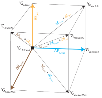
Figure 4: Superposition principle underlying DEF. Superposition of the projected absolute defect energies to obtain DEF end-member Gibbs energies, illustrated for (A,Vac)(B,Vac)(Vacⁱ,Aⁱ). As detailed in section II.3, the axes of the constitutional cube are formed by the A-vacancy, B-vacancy, and A-interstitial defect lines, shown by the blue, brown, and orange lines, respectively. The Gibbs energy of the DEF end-members on the constitutional cube is obtained from the superposition of the projected absolute defect energies, illustrated by defect basis vectors, onto the pristine end-member Gibbs energy, illustrated by the black square point.

We construct all defective DEF end-members with respect to the defect-free compound A_pB_q, ensuring that the mapping between the convex hull composition and DEF constitution space is physical in the dilute defect range. As detailed in sections II.2 and II.3, the pristine compound forms the origin of the DEF constitution space. In other words, the projected absolute defect energies measure the energy of defective end-members with respect to the pristine compound. Accordingly, the Gibbs energy of the pristine end-member must be added to all defective end-members. Therefore, for B-interstitial defects in A_pB_q, ${}^{0}G_{\text{A:B:B\textsuperscript{i}}}={}^{0}G_{\text{A:B:Vac}}+m\Delta E_{\text{\ce{B^i}}}$. The case of vacancies is slightly different. For example, for a defective A_pB_qwith A-vacancy defects, the defective end-member can be described as ${}^{0}G_{\text{Vac:B}}={}^{0}G_{\text{A:B}}-{}^{0}G_{\text{A:Vac}}={}^{0}G_{\text{A:B}}-{}^{0}G_{\text{A:B}}+{}^{0}G_{\text{Vac:B}}$. Note that the second equation gives the projection on the B-end; thus, the first two terms cancel out. The first equation gives the flipped projection on A-end for A-vacancy detailed in Ref.Anand et al. (2021) (see Figure 2).

For a B-antisite defect, the defective end-member energy can be described as

$$\begin{split}{}^{0}G_{\text{B:B}}&={}^{0}G_{\text{A:B}}-{}^{0}G_{\text{A:Vac}}+{}^{0}G_{\text{B:Vac}}\\ &=\overbrace{{}^{0}G_{\text{A:B}}}^{\text{\scriptsize{DEF origin}}}+\overbrace{(-{}^{0}G_{\text{A:B}}+{}^{0}G_{\text{Vac:B}})}^{\text{\scriptsize{B-end projection of A-vac}}}\\ &+\overbrace{{}^{0}G_{\text{B:Vac}}}^{\text{\scriptsize{B-end projection of B-interstitial}}}\\ &={}^{0}G_{\text{A:B}}+p\Delta E_{\text{\ce{Vac_A}}}+p\Delta E_{\text{\ce{B^i}}}\end{split}$$ (8)

Note that ${}^{0}G_{\text{Vac:B}}$ indicates the end-member containing A-vacancy, while ${}^{0}G_{\text{B:Vac}}$ shows the end-member containing B-interstitial. Therefore, a B-antisite defect can be considered a combination of these two individual defects (see Figure 3(b)).

For DEF end-members containing multiple defects, the superposition principle can be directly applied to the projected absolute defect energies. For example, for the Vac:Vac end-member, the absolute defect energy projections on the B-end and A-end are simply added so that:

$$\begin{split}{}{}^{0}G_{\text{Vac:Vac}}&=\overbrace{{}{}^{0}G_{\text{A:B}}}^{\text{\scriptsize{DEF origin}}}+\overbrace{(-{}^{0}G_{\text{A:B}}+{}{}^{0}G_{\text{Vac:B}})}^{\text{\scriptsize{B-end projection of A-vac}}}\\ &+\overbrace{(-{}{}^{0}G_{\text{A:B}}+{}{}^{0}G_{\text{A:Vac}})}^{\text{\scriptsize{A-end projection of B-vac}}}\\ &={}{}^{0}G_{\text{A:B}}+p\Delta E_{\text{A-vac}}+q\Delta E_{\text{B-vac}}\end{split}$$ (9)

Similarly, the Vac:Vac:Aⁱ in the three-sublattice model can be described as (see Figure 4)

$$\begin{split}&{}^{0}G_{\text{Vac:Vac:A\textsuperscript{i}}}=\overbrace{{}{}^{0}G_{\text{A:B}}}^{\text{\scriptsize{DEF origin}}}+\overbrace{(-{}^{0}G_{\text{A:B}}+{}^{0}G_{\text{Vac:B}})}^{\text{\scriptsize{B-end projection of A-vac}}}\\ &+\overbrace{(-{}^{0}G_{\text{A:B}}+{}{}^{0}G_{\text{A:Vac}})}^{\text{\scriptsize{A-end projection of B-vac}}}+\overbrace{{}{}^{0}G_{\text{Vac:Vac:A\textsuperscript{i}}}}^{\text{\scriptsize{A-end projection of B-interstitial}}}\\ &={}{}^{0}G_{\text{A:B}}+p\Delta E_{\text{A-vac}}+q\Delta E_{\text{B-vac}}+m\Delta E_{\text{\ce{B^i}}}\end{split}$$ (10)

The general derivation of the DEF end-member Gibbs energy aligns with our earlier derivation of DEF in Ref.Adekoya and Snyder (2024) as shown in Appendix A for an example vacancy defect.

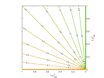
Figure 5: Mapping of the constitutional square for the (A,Vac)(B,Vac) DEF model, formed by ($1-y^{\text{1}}_{\text{vac}}$)-($1-y^{\text{2}}_{\text{vac}}$) axes, into the mole fraction composition $X_{B}$. $X_{B}=1$ and $X_{B}=0$ lines are shown by thick green and orange lines, respectively.

II.2 AB compound with dilute A-vacancy and B-vacancy

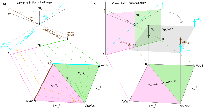
Figure 6: Mapping the composition and formation energy from a model convex hull (A-AB-B) to the constitutional square of a two-sublattice DEF model for A-vacancy and B-vacancy, (A, Vac)(B, Vac).Formation energies of defect-free AB ($\Delta H_{AB}$), defective AB with A-vacancy, and defective AB with B-vacancy are represented by the black square, blue circle, and brown diamond, respectively. The defect lines for A-vacancy and B-vacancy are indicated by the blue and brown lines, respectively. (a) Graphic representation of the mapping between $X_{B}$ on the convex hull and the constitutional square of the two-sublattice model. Physically relevant $X_{B}$ values for A-vacancy lie on the AB-B side (B-rich), colored green, and for B-vacancy lie on the A-AB side (A-rich), colored pink. The corresponding areas on the constitutional square for A-vacancy and B-vacancy are colored green and pink, respectively. (b) Graphic representation of the mapping between absolute defect energies, $\Delta E_{\text{VacA}}$ and $\Delta E_{\text{VacB}}$, and DEF end-members’ Gibbs energies. These defect energies measure the Gibbs energy of defective end-members relative to the pristine end-member A:B, as detailed in Section II.1.

In this section, we first derive the mapping between the composition space in a standard convex hull, $X$, and the constitutional space defined by the site fractions of constituents in the DEF sublattice model, $Y$, for the AB binary compound with dilute neutral vacancies, described by a two-sublattice model as (A,Vac)(B,Vac). The constitutional square consists of two axes, $y^{\text{1}}_{\text{vac}}$ and $y^{\text{2}}_{\text{vac}}$, denoting the site fractions of vacancies in the first and second sublattices, respectively. Within each sublattice, the total site fractions of distinct constituents equal one. Hence the site fractions of A and B, $y^{\text{1}}_{\text{A}}$ and $y^{\text{1}}_{\text{B}}$, follow $1-y^{\text{1}}_{\text{vac}}=y^{\text{1}}_{\text{A}}$ and $1-y^{\text{2}}_{\text{vac}}=y^{\text{1}}_{\text{B}}$. Therefore, the constitutional space of the two-sublattice model has two degrees of freedom. On the other hand, the composition of mole fractions of components in the $X$ space for a binary system has one degree of freedom. The $X$-composition of each component A or B per formula unit (or per mole of formula unit) can be related to the DEF site fractions using the following equations (see equation 1),

$$\begin{split}X_{A}&=\frac{y^{\text{1}}_{\text{A}}}{y^{\text{1}}_{\text{A}}+y^{\text{1}}_{\text{B}}}=\frac{1-y^{\text{1}}_{\text{vac}}}{(1-y^{\text{1}}_{\text{vac}})+(1-y^{\text{2}}_{\text{vac}})}\\ X_{B}&=\frac{y^{\text{1}}_{\text{B}}}{y^{\text{1}}_{\text{A}}+y^{\text{1}}_{\text{B}}}=\frac{1-y^{\text{2}}_{\text{vac}}}{(1-y^{\text{1}}_{\text{vac}})+(1-y^{\text{2}}_{\text{vac}})}\\ \end{split}$$ (11)

which provides the functional mapping between $X$ and $Y$. As shown in Figure 6(a), the mapping expands the 1-dimensional $X$-space, associated with two defects lines, A-vacancy, and B-vacancy, into the 2-dimensional constitutional square $Y$. In other words, the non-parallel A-vacancy and B-vacancy lines form the orthogonal basis vectors for the Y-space.

As shown in Figure 5, each line on the ($1-y^{\text{1}}_{\text{vac}}$)-($1-y^{\text{2}}_{\text{vac}}$) constitutional square maps into one point on $X_{B}$. The line at $y^{\text{1}}_{\text{vac}}=1$ corresponds to $X_{B}=1$ and the line at $y^{\text{2}}_{\text{vac}}=1$ corresponds to $X_{B}=0$. The diagonal line at $y^{\text{1}}_{\text{vac}}=y^{\text{2}}_{\text{vac}}$ corresponds to $X_{B}=\frac{1}{2}$. On these three lines exist 4 special points, constituting the end-members at $y^{\text{1}}_{\text{vac}}=1,y^{\text{2}}_{\text{vac}}=0$, corresponding to the Vac:B end-member, $y^{\text{1}}_{\text{vac}}=0,y^{\text{2}}_{\text{vac}}=1$, corresponding to the A:Vac end-member, $y^{\text{1}}_{\text{vac}}=0,y^{\text{2}}_{\text{vac}}=0$, corresponding to the A:B end-member, and $y^{\text{1}}_{\text{vac}}=1,y^{\text{2}}_{\text{vac}}=1$, corresponding to the Vac:Vac end-member (see Figure 6 and 5). Note that at $y^{\text{1}}_{\text{vac}}=1,y^{\text{2}}_{\text{vac}}=1$, $X_{B}$ is ill-defined and this point sits at the intersection of all constant $X_{B}$ contour lines (see Figure 5).

As illustrated in Figure 6(a), the AB-B segment of $X_{B}$, which includes the A-vacancy defect line extending from pristine AB to B (AB$\rightarrow$B) corresponds to the top-right triangular region within the $Y$-square. This region includes any combination of $y^{\text{1}}_{\text{vac}}$ and $y^{\text{2}}_{\text{vac}}$ as long as $y^{\text{1}}_{\text{vac}}\geq y^{\text{2}}_{\text{vac}}$. However, only the top edge of the $Y$-square (or line $y^{\text{2}}_{\text{vac}}=0$) corresponds to the A-vacancy defect line on the convex hull as it physically connects to an A-vacancy, forming A_1-$\delta$B in dilute ranges, without B-vacancy defects. Therefore, we map the A-vacancy line on the AB$\rightarrow$B segment of $X_{B}$ to the $y^{\text{2}}_{\text{vac}}=0$ line in the constitutional square, as shown by the blue line in Figure 6(a). Similarly, the A-AB segment of $X_{B}$, which includes the B-vacancy defect line extending from pristine AB to A, corresponds to the bottom-left triangular region within the $Y$-square. The only line on this triangle with a one-on-one mapping to B-vacancy without an A-vacancy is $y^{\text{1}}_{\text{vac}}=0$, forming the second basis vector of the $Y$ constitutional square (orange line in Figure 6(a)). The vertices of the constitutional square, $Y$, constitute the DEF end-members, for which there is a one-on-one correspondence to $X$ according to equation 11; A:B defined at $y^{\text{1}}_{\text{vac}}=1,y^{\text{2}}_{\text{vac}}=0$ (the origin of the $Y$-space) maps to $X_{B}=\frac{1}{2}$ or AB compound composition, Vac:B defined at $y^{\text{1}}_{\text{vac}}=1,y^{\text{2}}_{\text{vac}}=0$ maps to $X_{B}=1$ or B-end of the convex hull, and A:Vac defined at $y^{\text{1}}_{\text{vac}}=0,y^{\text{2}}_{\text{vac}}=1$ maps to $X_{B}=0$ or A-end of the convex hull. $X_{B}$ for Vac:Vac ($y^{\text{1}}_{\text{vac}}=1,y^{\text{2}}_{\text{vac}}=1$) is ill-defined. However, the Vac:Vac point in $Y$ sits at the intersections of all $X$-constant contours (or level lines) (see Figure 5) and, therefore, can be arbitrarily defined as the summation of any $X$ point. We define Vac:Vac as the sum of A:B, A:Vac and Vac:B which aligns with the superposition principle in the context of dilute defects (see equation 9).

As the mapping between $X_{B}$ and DEF end-members is established, we can relate DEF end-member Gibbs energies (per formula unit for AB) to defect absolute energies according to the procedure detailed in Section II.1, and shown in Figure 6(b)

$${}^{0}G_{\text{A:B}}=\mu_{A}^{0}+\mu_{B}^{0}+2\Delta H_{\text{f}}^{\text{AB}}$$

$${}^{0}G_{\text{A:Vac}}={}^{0}G_{\text{A:B}}+\Delta E_{\text{B-vacancy}}$$

$${}^{0}G_{\text{Vac:B}}={}^{0}G_{\text{A:B}}+\Delta E_{\text{A-vacancy}}$$

$${}^{0}G_{\text{Vac:Vac}}={}^{0}G_{\text{A:B}}+\Delta E_{\text{B-vacancy}}+\Delta E_{\text{A-vacancy}}$$ (12)

The DEF end-members Gibbs energies for a general binary compound A_pB_qis related to the absolute defect energies by

$$\begin{split}&{}^{0}G_{\text{A:B}}=p\mu_{A}^{0}+q\mu_{B}^{0}+(p+q)\Delta H_{\text{f}}^{\text{AB}}\\ &{}^{0}G_{\text{A:Vac}}={}^{0}G_{\text{A:B}}+q\Delta E_{\text{B-vacancy}}\\ &{}^{0}G_{\text{Vac:B}}={}^{0}G_{\text{A:B}}+p\Delta E_{\text{A-vacancy}}\\ &{}^{0}G_{\text{Vac:Vac}}={}^{0}G_{\text{A:B}}+p\Delta E_{\text{A-vacancy}}+q\Delta E_{\text{B-vacancy}}\\ \end{split}$$ (13)

The above equations follow the superposition principle underlying the thermodynamic conditions for individual isolated defects at dilute ranges, aligned with the DEF construct for dilute defects. For example, the Gibbs energy of Vac:Vac end-member (an end-member containing multiple defects) is the sum of the formation energies of both A-vacancy and B-vacancy (see equation 9). This represents a defective compound containing both A-vacancy and B-vacancy defects at dilute concentrations. The DEF end-member Gibbs energies from equation 13 can be substituted into equation 2 to obtain the Gibbs energy per formula unit of the defective compound.

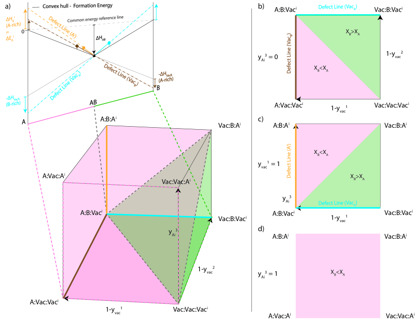
Figure 7: Mapping the composition and formation energy from a model convex hull (A-AB-B) to the constitutional cube of a three-sublattice DEF model for A-vacancy, B-vacancy, and A-interstitial. Formation energies of defect-free AB ($\Delta H_{AB}$) , defective AB with A-vacancy, defective AB with B-vacancy, and defective AB with A-interstitial are shown by the black square, blue circle, brown diamond, and orange hexagon, respectively. The defect lines for A-vacancy, B-vacancy, and A-interstitial are shown by the blue, brown, and orange lines, respectively. (a) Graphic representation of the mapping between $X_{B}$ on the convex hull and the constitutional cube of the three-sublattice model (or $Y$-space cube). The $X_{B}$ composition on the AB-B and A-AB sides maps into the green and pink regions of the $Y$-space cube, respectively. Lines on the constitutional cube that are physically relevant to the individual defect lines on the convex hull are shown by the respective colors of the defect lines, i.e., blue, brown, and orange for A-vacancy, B-vacancy, and A-interstitial. Projections of the constitutional cube into planes defined by (b) $y^{\text{3}}_{\text{A}^{\text{i}}}=0$, (c) $y^{\text{1}}_{\text{vac}}=1$ and (d) $y^{\text{3}}_{\text{A}^{\text{i}}}=1$.

II.3 AB compound with dilute A-vacancy, B-vacancy, and A-interstitial

Here, we describe the DEF for the binary AB compound with dilute ranges of neutral vacancies and a self-interstitial defect, described by a three-sublattice model as (A,Vac)(B,Vac)(Vacⁱ,Aⁱ). The first and second sublattices contain the A and B substitutional sites, hosting A, B, or vacancy defects, while the third sublattice contains interstitial sites, primarily occupied by vacancies and host secondary A-interstitial defects. The constitutional space (or $Y$-space) with 3 sublattices forms a cube with eight end-members (or eight vertices). As shown in Figure 7(a), the constitutional cube is formed by three axes (or three degrees of freedom), $y^{\text{1}}_{\text{vac}}$, $y^{\text{2}}_{\text{vac}}$, and $y^{\text{3}}_{\text{A}^{\text{i}}}$, denoting the site fractions of A- and B- vacancies and A-interstitial in the first, second, and third sublattices, respectively. Each of the non-parallel defect lines (A-vacancy, B-vacancy, or A-interstitial), all intersecting at the AB point on the convex hull, form one axis of the constitutional cube in the $Y$-space (see Figure 7(a)). The point of intersection, or the A:B:Vacⁱ serves as the origin for the $Y$-constitutional cube.

The $X$-composition of each component A or B per formula unit is related to the DEF site fractions using the following equations (see equation 1).

$$\begin{split}X_{A}&=\frac{y^{\text{1}}_{\text{A}}+y^{\text{3}}_{\text{A}^{\text{i}}}}{y^{\text{1}}_{\text{A}}+y^{\text{1}}_{\text{B}}+y^{\text{3}}_{\text{A}^{\text{i}}}}=\frac{(1-y^{\text{1}}_{\text{vac}})+y^{\text{3}}_{\text{A}^{\text{i}}}}{(1-y^{\text{1}}_{\text{vac}})+(1-y^{\text{2}}_{\text{vac}})+y^{\text{3}}_{\text{A}^{\text{i}}}}\\ X_{B}&=\frac{y^{\text{1}}_{\text{B}}}{y^{\text{1}}_{\text{A}}+y^{\text{1}}_{\text{B}}+y^{\text{3}}_{\text{A}^{\text{i}}}}=\frac{1-y^{\text{2}}_{\text{vac}}}{(1-y^{\text{1}}_{\text{vac}})+(1-y^{\text{2}}_{\text{vac}})+y^{\text{3}}_{\text{A}^{\text{i}}}}\\ \end{split}$$ (14)

which provide the mapping between the $X$- and $Y$- spaces. The mapping expands the 1-dimensional $X$-space associated with three defects lines, A-vacancy, B-vacancy, and A-interstitial, into a 3-dimensional constitutional cube, as shown in Figure 7(a). Figure 8 illustrates the $X_{B}$-constant contours (or level planes) on the $Y$-space (or constitutional cube of the DEF model).

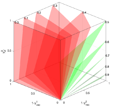
Figure 8: Mapping of the constitutional cube for the (A,Vac)(B,Vac)(Vacⁱ,Aⁱ) DEF model, formed by ($1-y^{\text{1}}_{\text{vac}}$)-($1-y^{\text{2}}_{\text{vac}}$)-$y^{\text{3}}_{\text{A}^{\text{i}}}$, into the mole fraction composition $X_{B}$. The contour level planes in the constitutional cube are labeled with corresponding $X_{B}$ values. Level planes for $X_{B}<0.5$ and $X_{B}\geq 0.5$ are colored red and green, respectively.

As shown in Figure 8, each plane on the ($1-y^{\text{1}}_{\text{vac}}$)-($1-y^{\text{2}}_{\text{vac}}$)-$y^{\text{3}}_{\text{A}^{\text{i}}}$ constitutional cube maps into one point on $X_{B}$. The face plane at $y^{\text{2}}_{\text{vac}}=1$ corresponds to $X_{B}=0$, and the body diagonal plane, formed by $y^{\text{1}}_{\text{vac}}=y^{\text{2}}_{\text{vac}}$ and $1-y^{\text{2}}_{\text{vac}}=y^{\text{3}}_{\text{A}^{\text{i}}}$ lines, corresponds to $X_{B}=\frac{1}{2}$. The plane corresponding to $X_{B}=1$ collapses into the line at $y^{\text{1}}_{\text{vac}}=1$ and $y^{\text{3}}_{\text{A}^{\text{i}}}=0$. Note that the plane at $y^{\text{3}}_{\text{A}^{\text{i}}}=0$ replicates the composition square for the (A,Vac)(B,Vac) model detailed in section II.2.

To map the defect formation energy from the convex hull to the corresponding end-member Gibbs energy, ${}^{0}G_{\text{end}}$ , on the constitutional cube, we first identify the physically relevant lines on the $Y$-cube to the $X_{B}$ values for each defect line. As shown in Figure 7(a), both the B-vacancy and A-interstitial defect lines lie on the A-AB side of $X_{B}$ on the convex hull and, as expected by the $X$-$Y$ mapping of equation 14, their physically relevant $Y$-lines span over the $X_{B}<X_{A}$ region on the $Y$-cube (colored red in Figure 7(a)). On the other hand, the A-vacancy defect line lies on the AB-B side of $X_{B}$, and thus its physically relevant $Y$-line maps into the $X_{B}>X_{A}$ region on the $Y$-cube (colored green in Figure 7(a)). As shown in Figure7(a), the lines at $y^{\text{2}}_{\text{vac}}=0$ and $y^{\text{3}}_{\text{A}^{\text{i}}}=0$, $y^{\text{1}}_{\text{vac}}=0$ and $y^{\text{3}}_{\text{A}^{\text{i}}}=0$, and $y^{\text{2}}_{\text{vac}}=0$ and $y^{\text{1}}_{\text{vac}}=0$, corresponds to the physically relevant $Y$-value for A-vacancy, B-vacancy, and A-interstitial defect lines, respectively. As shown in Figure 7(a), these are the basis vectors (axes) on the $Y$-constitutional cube, and each axis represents a single defect type at different concentrations in the dilute ranges of isolated defects. As shown in Figure 7(a), the origin for the $Y$-constitutional cube, or the A:B:Vacⁱ end-member, corresponds to the defect-free AB compound with the formation energy of $\Delta H_{\text{f}}^{\text{AB}}$. Other end-members are obtained by extending the origin along the three axes of $Y$-cube, corresponding to A:B:Aⁱ for A-interstitial axis, Vac:B:Vacⁱ for A-vacancy axis, and A:Vac:Vacⁱ for B-vacancy axis. The DEF end-member Gibbs energies for the AB binary compound with A-vacancy, B-vacancy, and A-interstitial defects are

$${}^{0}G_{\text{A:B:Vac\textsuperscript{i}}}=\mu_{A}^{0}+\mu_{B}^{0}+2\Delta H_{\text{f}}^{\text{AB}}$$

$${}^{0}G_{\text{A:Vac:Vac\textsuperscript{i}}}={}^{0}G_{\text{A:B:Vac\textsuperscript{i}}}+\Delta E_{\text{B-vacancy}}$$

$${}^{0}G_{\text{Vac:B:Vac\textsuperscript{i}}}={}^{0}G_{\text{A:B:Vac\textsuperscript{i}}}+\Delta E_{\text{A-vacancy}}$$

$${}^{0}G_{\text{Vac:Vac:Vac\textsuperscript{i}}}={}{}^{0}G_{\text{A:B:Vac\textsuperscript{i}}}+\Delta E_{\text{B-vacancy}}+\Delta E_{\text{A-vacancy}}$$

$${}^{0}G_{\text{A:B:A\textsuperscript{i}}}={}{}^{0}G_{\text{A:B:Vac\textsuperscript{i}}}+\Delta E_{A^{i}}$$

$${}^{0}G_{\text{A:Vac:A\textsuperscript{i}}}={}^{0}G_{\text{A:B:Vac\textsuperscript{i}}}+\Delta E_{\text{B-vacancy}}+\Delta E_{A^{i}}$$

$${}^{0}G_{\text{Vac:B:A\textsuperscript{i}}}={}^{0}G_{\text{A:B:Vac\textsuperscript{i}}}+\Delta E_{\text{A-vacancy}}+\Delta E_{A^{i}}$$

$${}^{0}G_{\text{Vac:Vac:A\textsuperscript{i}}}={}^{0}G_{\text{A:B:Vac\textsuperscript{i}}}+\Delta E_{\text{B-vacancy}}$$

$$\hskip 56.9055pt+\Delta E_{\text{A-vacancy}}+\Delta E_{A^{i}}$$ (15)

For a general binary compound A_pB_qwith a DEF sublattie model of (A,Vac)_p(B,Vac)_q(Vacⁱ,Aⁱ)_m, the end-member Gibbs energies are

$${}^{0}G_{\text{A:B:Vac\textsuperscript{i}}}=p\mu_{A}^{0}+q\mu_{B}^{0}+(p+q)\Delta H_{\text{f}}^{\text{AB}}$$

$${}^{0}G_{\text{A:Vac:Vac\textsuperscript{i}}}={}^{0}G_{\text{A:B:Vac\textsuperscript{i}}}+q\Delta E_{\text{B-vacancy}}$$

$${}^{0}G_{\text{Vac:B:Vac\textsuperscript{i}}}={}^{0}G_{\text{A:B:Vac\textsuperscript{i}}}+p\Delta E_{\text{A-vacancy}}$$

$${}^{0}G_{\text{Vac:Vac:Vac\textsuperscript{i}}}={}^{0}G_{\text{A:B:Vac\textsuperscript{i}}}+q\Delta E_{\text{B-vacancy}}+p\Delta E_{\text{A-vacancy}}$$

$${}^{0}G_{\text{A:B:A\textsuperscript{i}}}={}^{0}G_{\text{A:B:Vac\textsuperscript{i}}}+m\Delta E_{A^{i}}$$

$${}^{0}G_{\text{A:Vac:A\textsuperscript{i}}}={}^{0}G_{\text{A:B:Vac\textsuperscript{i}}}+q\Delta E_{\text{B-vacancy}}+m\Delta E_{A^{i}}$$

$${}^{0}G_{\text{Vac:B:A\textsuperscript{i}}}={}^{0}G_{\text{A:B:Vac\textsuperscript{i}}}+p\Delta E_{\text{A-vacancy}}+m\Delta E_{A^{i}}$$

$${}^{0}G_{\text{Vac:Vac:A\textsuperscript{i}}}={}^{0}G_{\text{A:B:Vac\textsuperscript{i}}}+q\Delta E_{\text{B-vacancy}}$$

$$\hskip 56.9055pt+p\Delta E_{\text{A-vacancy}}+m\Delta E_{A^{i}}$$ (16)

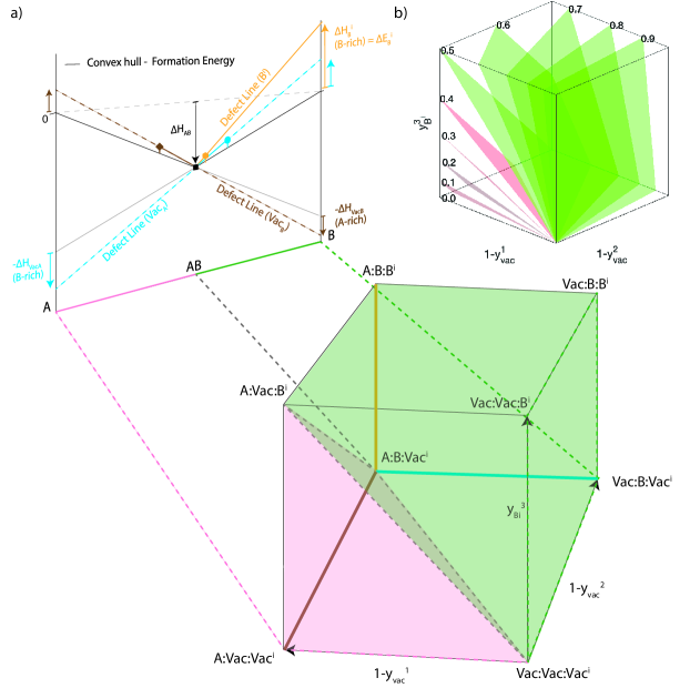
Figure A1: (a) Graphic representation of the mapping between $X_{B}$ composition on the convex hull and the constitutional cube of the three-sublattice model ($Y$-space cube). The $X_{B}$ composition on the AB-B and A-AB sides maps into the green and pink regions of the $Y$-space cube, respectively. Lines on the constitutional cube relevant to the defect lines on the convex hull are shown in the respective colors: blue for A-vacancy, brown for B-vacancy, and orange for B-interstitial. (b) Mapping of the constitutional cube for the (A,Vac)(B,Vac)(Vacⁱ,Bⁱ) DEF model, ($1-y^{\text{1}}_{\text{vac}}$)-($1-y^{\text{2}}_{\text{vac}}$)-$y^{\text{3}}_{\text{A}^{\text{i}}}$, into the composition $X_{B}$. Contour planes in the constitutional cube are labeled with corresponding $X_{B}$ values. Contour planes for $X_{B}<0.5$ and $X_{B}\geq 0.5$ are colored red and green, respectively.

A similar DEF model for the B-interstitial defect, (A,Vac)(B,Vac)(Vacⁱ,Bⁱ) is illustrated in Appendix Figure A1. The general recipe for constructing a typical DEF model for neutral defects is provided in section IV.

III Defect Energy Formalism for Charged Defects

For a compound with charged defects, the concentration of defects is controlled by the Fermi level through the charge neutrality condition

$$0=n-p-\sum_{d,q}q_{d}c_{d}$$ (17)

where $n$, $p$ and $c_{d}$ are the concentration of free electrons, holes, and defect $d$ with a net charge of $q_{d}$ (e.g., +2 for a doubly ionized donor with 2 electrons removed or -2 for an acceptor with 2 electrons added), respectively. $k$ and $T$ are the Boltzmann constant and temperature. $n$ and $p$ are a function of the Fermi level, while $c_{d}$ is a function of both the Fermi level and chemical potential. The concentration of electrons and holes for non-degenerate semiconductors, with the Fermi level several $kT$ below the conduction band, follows the Boltzmann distribution Sze and Ng (2006)

$$\begin{split}n&=N_{c}\exp{\left(-\frac{E_{c}-E_{f}}{kT}\right)}\\ p&=N_{v}\exp{\left(-\frac{E_{f}-E_{v}}{kT}\right)}\end{split}$$ (18)

where $N_{v}$ ($N_{c}$) is the effective density of states in the valence (conduction) band, and $E_{f}$, $E_{c}$, and $E_{v}$ denote the Fermi level, the conduction band minimum, and the valance band maximum energies, respectively. The effective density of states (per volume) in the valence and conduction band are given by $N_{v}=2\left(\frac{2\pi m^{*}_{h}kT}{h^{2}}\right)^{3/2}$ and $N_{c}=2\left(\frac{2\pi m^{*}_{e}kT}{h^{2}}\right)^{3/2}$, where $h$ is the Plank’s constant, $m^{*}_{h}$ and $m^{*}_{e}$ are the effective masses of holes and electrons at the valence band and conduction band edges, respectively. Multiplying $N_{v}$ and $N_{c}$ in the volume per formula unit of the compound, $V_{0}$, counts the effective densities per formula unit (e.g., see Ref. Chen et al. (1998); Peters et al. (2019)), which we consider in this work. Note that according to equation 18, the product of $n$ and $p$ is constant and independent of $E_{f}$, given by $np=N_{c}N_{v}\exp{\left(-\frac{E_{g}}{kT}\right)}$, where $E_{g}=E_{c}-E_{v}$ is the band gap of the defect-free compound.

The concentration of defect $d$ in the dilute range, $c_{d}$, is given by the Arrhenius relation Freysoldt et al. (2014)

$$c_{d}^{q}=c_{0}\exp{\left(-\frac{\Delta H_{\text{d}}^{q}}{kT}\right)}$$ (19)

where $c_{0}$ denotes the concentration of possible defect sites in the host compound and $\Delta H_{\text{d}}^{\text{q}}$ denotes the grand-canonical formation energy for the defect $d$ with a net charge of $q$, which in addition to chemical potential depends on $E_{f}$ according to the following equation.

$$\Delta H_{d}^{q}=E_{\text{def}}^{q}-E_{\text{pristine}}-\sum\Delta N_{i}\mu_{i}+qE_{f}$$ (20)

Here, $E_{\text{def}}^{q}$ and $E_{\text{pristine}}$ denote the energies of the defective and pristine structures, respectively, where the defective structure has a net charge of $q$. $\Delta N_{i}$ is the number of atoms of species $i$ added to or removed from the defective structure (e.g., +1 for interstitials, -1 for vacancies) and $\mu_{i}$ is the chemical potential of the species $i$.

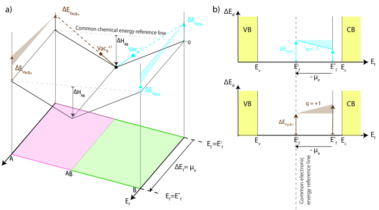
Figure 9: Formation energy convex hull in the composition-Fermi level space ($X-E_{f}$). a) Graphical illustration of a typical A-AB-B convex hull along the Fermi level and chemical composition. The A-AB-A convex hull, including the A+AB and AB+B common tangent lines, is independent of the Fermi level because it consists of charge neutral compounds, resulting in a flat extrusion of the A-AB-B hull along $E_{f}$. In contrast, the energy of a defected compound with a net charge $q$ depends on $E_{f}$ and varies with a slope of $q$ along $E_{f}$, as shown by shaded triangles. The absolute defect energy of defected AB ($\Delta E_{\text{d}}$) are shown for A-vacancy with $q=-1$ and B-vacancy with $q=+1$. b) Graphical representation of unifying the electronic energy reference for charge carriers and ionic defects. The convex hull at the equilibrium Fermi level ($E_{f}^{*}$) is shifted to the intrinsic Fermi level ($E_{f}^{i}$). The chemical-potential-independent absolute defect energy is shifted by $-q\mu_{e}$ (see equation 25).

The equilibrium Fermi level, $E^{*}_{f}$, is uniquely determined by solving the charge neutrality condition of equation 17 for $E_{f}$. As shown in Figure 9(a), the equilibrium Fermi level can be associated to a plane on the formation energy convex hull in the composition-Fermi level space ($X-E_{f}$). The formation energy of defect $d$ varies with $E_{f}$ with a slope of $q$ according to equation 20. Therefore, the charge state of defect $d$ is implicitly determined by $E_{f}^{*}$, where different charge states of a given defect $d$ enter the charge neutrality condition of equation 17. The equilibrium Fermi level $E^{*}_{f}$ is a measure of the chemical potential of electrons at equilibrium, $\mu_{e}$ (i.e., $\mu_{e}=E^{*}_{f}$) See (2009), defined as the Gibbs energy required to add or remove an electron from the compound.

We define the standard chemical potential for electrons and holes, $\mu_{e}^{0}$ and $\mu_{h}^{0}$, respectively, for the Fermi level of the intrinsic case or a defect-free compound. Therefore, $\mu_{e}^{0}$ and $\mu_{h}^{0}$ represent the Gibbs energy change for creation of an electron and hole through the electron-hole pair reaction ($\text{e}\textsuperscript{-}+\text{h}\textsuperscript{+}\longleftrightarrow 0$) in the absence of any ionic defect. The electron-hole pair reaction implies that $\mu_{e}^{0}+\mu_{h}^{0}=0$ at equilibrium. The intrinsic Fermi level is simply determined through $n=p$ (see equation 17), resulting in $E_{f}^{i}=\frac{E_{v}+E_{c}}{2}-\frac{kT}{2}\ln(\frac{N_{c}}{N_{v}})$. We consider the intrinsic Fermi level as the reference electronic energy in the DEF framework because it corresponds to a defect-free compound with a net charge of zero. This choice for the reference electronic state is consistent with the choice for the reference chemical state corresponding to the defect-free compound (see section II.1). Setting $E_{f}^{i}=0$ results in $E_{c}=\frac{E_{g}}{2}+\frac{kT}{2}\ln\left(\frac{N_{c}}{N_{v}}\right)$ and $E_{v}=-\frac{E_{g}}{2}+\frac{kT}{2}\ln\left(\frac{N_{c}}{N_{v}}\right)$. The standard chemical potential of an electron is the Gibbs energy change due to adding an electron to the conduction band minimum, with the energy term equal to $\frac{E_{g}}{2}+\frac{kT}{2}\ln\left(\frac{N_{c}}{N_{v}}\right)$ and the entropy contribution term equal to $-kT\ln N_{c}$, corresponding to the selection of an electron site among $N_{c}$ available sites. Therefore, $\mu_{e}^{0}=\frac{E_{g}}{2}+\frac{kT}{2}\ln\left(\frac{N_{c}}{N_{v}}\right)-kT\ln N_{c}$. Similarly, the standard chemical potential for a hole is equal to the energy for removing an electron from the valence band with an entropy term corresponding to selection of a candidate hole site among $N_{v}$ available sites, resulting in $\mu_{h}^{0}=\frac{E_{g}}{2}-\frac{kT}{2}\ln\left(\frac{N_{c}}{N_{v}}\right)-kT\ln N_{v}$.

For the general case of a defected compound (non-intrinsic, non-degenerate), the shift in the equilibrium Fermi level $E_{f}^{*}$ with respect to the intrinsic Fermi level $E_{f}^{i}$, $\Delta E_{f}$, measures the chemical potential of electrons ($\Delta E_{f}=\mu_{e}$) according to the following equation (rearrangement of equation 18)

$$n=N_{c}\exp{\left(-\frac{E_{c}-(E_{f}^{i}+\Delta E_{f})}{kT}\right)}$$

$$=N_{c}\exp{\left(-\frac{(E_{c}-E_{f}^{i})}{kT}\right)\exp\left(-\frac{\mu_{e}}{kT}\right)}$$

$$\rightarrow \mu_{e}=\left[\frac{E_{g}}{2}+\frac{kT}{2}\ln\left(\frac{N_{c}}{N_{v}}\right)-kT\ln(Nc)\right]+kT\ln n$$

$$\rightarrow \mu_{e}=\mu_{e}^{0}+kT\ln n$$ (21)

Similarly, the chemical potential of holes is given by ($\Delta E_{f}=-\mu_{h}$)

$$p=N_{v}\exp{\left(-\frac{(E_{f}^{i}+\Delta E_{f})-E_{v}}{kT}\right)}$$

$$=N_{v}\exp{\left(-\frac{(E_{f}^{i}-E_{v})}{kT}\right)\exp\left(\frac{\mu_{h}}{kT}\right)}$$

$$\rightarrow \mu_{h}=\left[\frac{E_{g}}{2}-\frac{kT}{2}\ln\left(\frac{N_{c}}{N_{v}}\right)-kT\ln(Nv)\right]+kT\ln p$$

$$\rightarrow \mu_{h}=\mu_{h}^{0}+kT\ln p$$ (22)

Note that according to the above equation, $\mu_{e}+\mu_{h}=0$ is always satisfied, considering that $np=N_{c}N_{v}\exp{\left(-\frac{E_{g}}{kT}\right)}$.

The DEF construction for defected phases with charged defects includes an auxiliary sublattice to host electronic constituents, including free electrons and holes. Including the auxiliary sublattice besides the regular atomic (or ionic) sublattices is essential for determining the concentration of charge carriers, as is usually desired in the thermodynamic description of semiconductors. Existing studies in the literature have used the CEF both with or without including the charge carrier sublattice. The charge carrier sublattice represents the electron reservoir and thus facilitates the exchange of electrons to or from the regular atomic sublattices in a grand-canonical description. The number of available sites (per formula unit of the compound) on the free electron or hole sublattice are $N_{c}$ and $N_{v}$, respectively. Therefore, one may consider a DEF model with separate sublattices for free electrons and holes such as (A,Vac^-1)(B,A⁺¹)(Vac,e^-)${}_{N_{c}}$(Vac,h⁺)${}_{N_{v}}$. However, this representation makes the modeling complex as $N_{c}$ and $N_{v}$ can vary with compositions or by adding new chemical components to the system. Therefore, as recommended by other CEF studies Chen and Hillert (1996); Chen et al. (1998); Hillert (2001), we set the number of sites in the free electron and hole sublattices equal. Chen and Hillert Chen and Hillert (1996) compensate for the incorrect number of sites in the charge carrier sublattices by subtracting the terms $RT\ln N_{c}$ and $RT\ln N_{v}$ from the Gibbs formation energy of electrons and holes, respectively (see section 4 in Ref. Chen and Hillert (1996) for details). As shown in equation III, these correction terms have emerged in the derivation of $\mu_{e}^{0}$ and $\mu_{h}^{0}$, and are inherently embedded in the DEF formalism as detailed below. Therefore, the DEF model can be simplified to host free electrons and holes on a common sublattice as (A,Vac^-1)(B,A⁺¹)(Vac,e^-,h⁺).

The Gibbs energy per formula unit of the compound with charged defects is defined similar to a compound with neutral defects consisting of the surface of reference energy, $G^{\text{s.r.}}$, and the ideal mixing term for each sublattice. The additional Gibbs energy terms due to the charge carrier sublattice can be formulated as the following (after section 4 in Ref. Chen and Hillert (1996))

$$G_{\text{fu}}= G_{\text{fu}}^{\text{at}}+G_{\text{fu}}^{\text{ax}}$$

$$= G_{\text{fu}}^{\text{at}}+\overbrace{\sum\sum y_{\text{i}}y_{\text{j}}}^{=1}[({}^{0}G_{\text{i:j:e\textsuperscript{-}}}-{}^{0}G_{\text{i:j:vac}})y^{\text{3}}_{\text{e\textsubscript{-}}}$$

$$\hskip 42.67912pt+({}^{0}G_{\text{i:j:h\textsuperscript{+}}}-{}^{0}G_{\text{i:j:vac}})y^{\text{3}}_{\text{h\textsubscript{+}}}]$$

$$+kT\left(y^{\text{3}}_{\text{e\textsubscript{-}}}\ln(y^{\text{3}}_{\text{e\textsubscript{-}}})+y^{\text{3}}_{\text{h\textsubscript{+}}}\ln(y^{\text{3}}_{\text{h\textsubscript{+}}})+y^{\text{3}}_{\text{vac}}\ln(y^{\text{3}}_{\text{vac}})\right)$$

$$= G_{\text{fu}}^{\text{at}}+y^{\text{3}}_{\text{e\textsubscript{-}}}\underbrace{\left[({}^{0}G_{\text{i:j:e\textsuperscript{-}}}-{}^{0}G_{\text{i:j:vac}})+kT\ln(y^{\text{3}}_{\text{e\textsubscript{-}}})\right]}_{\mu_{e}}$$

$$+y^{\text{3}}_{\text{h\textsubscript{+}}}\underbrace{\left[({}{}^{0}G_{\text{i:j:h\textsuperscript{+}}}-{}^{0}G_{\text{i:j:vac}})+kT\ln(y^{\text{3}}_{\text{h\textsubscript{+}}})\right]}_{\mu_{h}}$$

$$+kTy^{\text{3}}_{\text{vac}}\ln(y^{\text{3}}_{\text{vac}})$$ (23)

where $G_{\text{fu}}^{\text{at}}$ is the Gibbs energy for a DEF model that only consists of the atomic sublattices (see equation 2) and $G_{\text{fu}}^{\text{ax}}$ is the additional Gibbs energy due to the charge carrier (or auxiliary) sublattice. $i$ and $j$ run over end-members that are formed by the atomic sublattices only and thus $\sum\sum y_{\text{i}}y_{\text{j}}=1$. Additionally, in deriving equation III, terms such as ${}^{0}{G}_{\text{i:j:vac}}\times y_{\text{i}}y_{\text{j}}y^{\text{3}}_{\text{vac}}$ are rearranged as ${}^{0}G_{\text{i:j:vac}}\times\left[y_{\text{i}}y_{\text{j}}(1-y^{\text{3}}_{\text{e\textsubscript{-}}}-y^{\text{3}}_{\text{h\textsubscript{+}}})\right]={}^{0}G_{\text{i:j}}\times y_{\text{i}}y_{\text{j}}(1)-{{}^{0}G}_{\text{i:j:vac}}\times y_{\text{i}}y_{\text{j}}(y^{\text{3}}_{\text{e\textsubscript{-}}}+y^{\text{3}}_{\text{h\textsubscript{+}}})$, where the first term is incorporated into $G_{\text{fu}}^{\text{at}}$ and the second term is embedded into $G_{\text{fu}}^{\text{ax}}$. $G_{\text{fu}}^{\text{at}}$ is the Gibbs energy for a DEF without considering the auxiliary charge carrier sublattice, and is given by $G_{\text{fu}}^{\text{at}}=\sum\sum{}^{0}G_{\text{i:j}}y_{\text{i}}y_{\text{j}}+kT\sum_{s}\sum_{k}y_{k}\ln(y_{k})$. $i$ and $j$ run over end-members that are formed by the atomic sublattices only, $s$ only runs over atomic sublattices, and $k$ runs over constituents of sublattice $s$. In the DEF formalism, Gibbs energy of defective end-members describing ionic defects with a non-zero net charge are parameterized as the sum of neutral defect formation energy and the ionization energy (as detailed below).

Within $G_{\text{fu}}^{\text{ax}}$ formulation, the chemical potential of free electrons ($\mu_{e}$) and holes ($\mu_{h}$) naturally arise, directly linking the DEF end-members with charge carriers to the chemical potentials of electrons and holes. For example, the term $({}^{0}G_{\text{i:j:h\textsuperscript{+}}}-{}^{0}G_{\text{i:j:vac}})+kT\ln(y^{\text{3}}_{\text{h\textsubscript{+}}})$ in the DEF Gibbs energy corresponds to $\mu_{h}^{0}+kT\ln p$ in equation III. In deriving this equality, we use the following equation

$$\begin{split}&\frac{p}{N_{v}}=\left(\frac{p}{N_{v}}N_{v}\right)\frac{1}{N_{v}}=\left(\frac{y^{\text{3}}_{\text{h\textsubscript{+}}}}{\underbrace{y^{\text{3}}_{\text{h\textsubscript{+}}}+y^{\text{3}}_{\text{e\textsubscript{-}}}+y^{\text{3}}_{\text{vac}}}_{1}}\right)\frac{1}{N_{v}}\\ &kT\ln(\frac{p}{N_{v}})=kT\ln y^{\text{3}}_{\text{h\textsubscript{+}}}-kT\ln N_{v}\rightarrow kT\ln p=kT\ln y^{\text{3}}_{\text{h\textsubscript{+}}}\end{split}$$ (24)

The direct connection between the chemical potential of electrons and holes and the DEF Gibbs energy formulation implies that the end-member Gibbs energy value, $(^{0}G_{\text{i:j:h\textsuperscript{+}}}-^{0}G_{\text{i:j:vac}})$, associated with formation of a hole, is $\mu_{h}^{0}$. The mixing entropy term associated with the vacant sites on the auxiliary sublattice (last term in equation III) approaches zero for low concentration of charge carriers, when $y^{\text{3}}_{\text{vac}}\rightarrow 1$ ($\lim_{X\to 0}(1-X)\ln(1-X)=-X$), and thus can be neglected.

Considering separate sublattices for free electrons and holes results in the same DEF Gibbs energy formulation as using a common sublattice for both. For separate sublattices, additional terms of the form $(^{0}G_{\text{i:j:e\textsuperscript{-}:h\textsuperscript{+}}}-^{0}G_{\text{i:j:vac:vac}})$ appear in the DEF Gibbs energy of equation III. This term represents the Gibbs energy for an electron-hole pair formation ($\text{e}\textsuperscript{-}+\text{h}\textsuperscript{+}\longleftrightarrow 0$), which is equal to zero at thermal equilibrium, making the Gibbs energy formulation the same as a single sublattice hosting electrons and holes. Additionally, terms of the form $y_{\text{i}}y_{\text{j}}y^{\text{3}}_{\text{vac}}y^{\text{4}}_{\text{vac}}{}^{0}G_{\text{i:j:vac:vac}}$ appear that can be rearranged as $y_{\text{i}}y_{\text{j}}(1-y^{\text{3}}_{\text{e\textsubscript{-}}})(1-y^{\text{4}}_{\text{h\textsubscript{+}}}){}^{0}G_{\text{i:j:vac:vac}}=y_{\text{i}}y_{\text{j}}{}^{0}G_{\text{i:j}}-y_{\text{i}}y_{\text{j}}y^{\text{3}}_{\text{e\textsubscript{-}}}{}^{0}G_{\text{i:j:vac:vac}}-y_{\text{i}}y_{\text{j}}y^{\text{4}}_{\text{h\textsubscript{+}}}{}^{0}G_{\text{i:j:vac:vac}}+y_{\text{i}}y_{\text{j}}(y^{\text{3}}_{\text{e\textsubscript{-}}}y^{\text{3}}_{\text{h\textsubscript{+}}}){}^{0}G_{\text{i:j:vac:vac}}$, to give the same formulation as for the common auxiliary sublattice in equation III. Note that the last term can be neglected because both $y^{\text{3}}_{\text{e\textsubscript{-}}}$ and $y^{\text{3}}_{\text{h\textsubscript{+}}}$ are small in the dilute range.

Within the DEF Gibbs energy formulation of equation III, energy contributions associated with ionized atomic defects must be relative to the reference electronic energy state, same as charge carriers, which we defined as the intrinsic Fermi level, $E_{f}^{i}$. Similar to unifying the chemical energy reference line for neutral defects (see section II.1), the formation energy of equation 20 must be shifted by $-q(E_{f}^{*}-E_{f}^{i})$ to unify the electronic energy reference line (see Figure 9(b)). Accordingly, the absolute defect energy of a defect $d$ with a net charge of $q$ with a unified chemical and electronic reference state is defined as

$$\begin{split}&\underbrace{\Delta H_{d}^{q}+\sum N_{i}\mu_{i}}_{\Delta E_{d}^{q}}-q\underbrace{(E_{f}^{*}-E_{f}^{i})}_{\mu_{e}}=E_{\text{def}}^{q}-E_{\text{pristine}}+q(E_{f}^{i})\\ &=\overbrace{\underbrace{E_{\text{def}}^{q}-E_{\text{def}}^{\emptyset}}_{\text{ionization energy}}+\underbrace{E_{\text{def}}^{\emptyset}-E_{\text{pristine}}}_{\text{neutral defect energy}}}^{\Delta E_{d}^{q}}\\ &\hskip 85.35826pt+q(E_{v}+\frac{E_{g}}{2}-\frac{kT}{2}\ln(\frac{N_{c}}{N_{v}}))\end{split}$$ (25)

where $E_{\text{def}}^{\emptyset}$ denotes the energy of the charge-neutral defective compound. Typical DFT total energy calculations directly compute the sum of neutral defect and ionization energies. The intrinsic Fermi level is formulated in terms of $E_{v}$ and $E_{g}$, typically obtained from DFT calculations. The defect energy on the right hand side of equation 25 is independent of the equilibrium Fermi level and chemical potential.

The chemical-potential and Fermi-level-independent defect energy of equation 25 is directly connected to the DEF end-member Gibbs energy. For example, consider the (A,Vac^-1)(B,A⁺¹)(Vac,e^-,h⁺) model, with a cationic A-vacancy on the first atomic sublattice and an anionic A-antisite on the second. The end-member A:A⁺¹:Vac associates with a defective compound with dilute anionic A-antisite defects and its Gibbs energy equals ${}^{0}G_{A:A\textsuperscript{+1}:Vac}={}^{0}G_{A:B:Vac}+(E_{\text{A-antisite}}^{+}-E_{\text{pristine}})+(E_{v}+\frac{E_{g}}{2}-\frac{kT}{2}\ln(\frac{N_{c}}{N_{v}}))$. The superposition principle is applied to derive the Gibbs energy of end-members that include both charged ionic defects in the atomic sublattices and charge carriers in the auxiliary sublattice. For example, ${}^{0}G_{A:A\textsuperscript{+1}:e\textsuperscript{-}}={}^{0}G_{A:B:Vac}+(E_{\text{A-antisite}}^{+}-E_{\text{pristine}})+(E_{v}+\frac{E_{g}}{2}-\frac{kT}{2}\ln(\frac{N_{c}}{N_{v}}))+\mu_{e}^{0}={}^{0}G_{A:B:Vac}+\Delta E_{\text{A-antisite}}^{+}+(E_{v}+E_{g})$.

III.1 AB compound with dilute charged A-vacancy and B-vacancy

In the following section, we elaborate on mapping the composition and defect formation energies onto the constitutional space and Gibbs energy of the DEF model for a compound with charged defects. To better understand the importance of the auxiliary charge carrier sublattice in the DEF model, we first consider a DEF model without the auxiliary sublattice for the AB binary compound with dilute charged vacancies, described by two ionic (or atomic) sublattices (A,Vac^-2)(B,Vac⁺²). The first and second sublattices contain A and B substitutional sites, respectively, hosting A, B, or charged vacancy defects. As shown in Figure 10(a), the constitutional space (or $Y$-space) forms a square with four end-members, described by two axes, $y^{\text{1}}_{\text{vac}}$ and $y^{\text{2}}_{\text{vac}}$, representing the site fractions of A and B vacancies in the first and second sublattices, respectively. Similar to neutral defects, each of the non-parallel defect lines (A-vacancy and B-vacancy) intersecting at the AB point on the convex hull forms one axis of the $Y$ constitutional square. Unlike neutral defects, the charge neutrality condition imposes an additional constraint on the mapping between the composition space ($X$) and the constitutional space of DEF ($Y$).

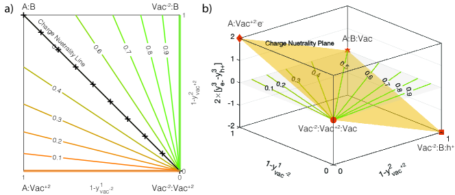
Figure 10: The DEF constitutional space with and without the auxiliary charge carrier sublattice. (a) The constitutional square for the (A,Vac^-2)(B,Vac⁺²) DEF model, mapped to the binary system composition, $X_{B}$. The $X_{B}=1$ and $X_{B}=0$ lines are shown in thick green and orange, respectively. Charge neutrality is only satisfied along the hatched black line. b) The constitutional cube for the (A,Vac^-2)(B,Vac⁺²)(Vac,e^-,h⁺) DEF model, with basis axes ($1-y^{\text{1}}_{\text{vac}}$), ($1-y^{\text{2}}_{\text{vac}}$), ($y^{\text{3}}_{\text{e\textsubscript{-}}}-y^{\text{3}}_{\text{h\textsubscript{+}}}$). Charge neutrality is satisfied across the orange plane. Contour lines for constant $X_{B}$ values are projected on the $(y^{\text{3}}_{\text{e\textsubscript{-}}}$-$y^{\text{3}}_{\text{h\textsubscript{+}}})=0$ plane. The top ($(y^{\text{3}}_{\text{e\textsubscript{-}}}$-$y^{\text{3}}_{\text{h\textsubscript{+}}})=1$) and bottom ($(y^{\text{3}}_{\text{e\textsubscript{-}}}$-$y^{\text{3}}_{\text{h\textsubscript{+}}})=-1$) planes contain end-members with free electrons and holes, respectively. The four corners of the charge neutrality plane, marked in red, are physically connected to the absolute defect energy projections on the convex hull at equilibrium Fermi energy.

The $X$-composition of A or B relates to the DEF site fractions as per equation 11 similar to neutral defects. However, enforcing charge neutrality constrains the $Y$-space square into the neutrality line, where $y^{\text{1}}_{\text{vac}}=y^{\text{2}}_{\text{vac}}$, as shown in Figure 10(a). Note that A:B and Vac^-2:Vac⁺² end-members are charge-neutral, while Vac^-2:B and A:Vac⁺² have a net charge. The neutrality line restricts the mapping between $X$ and $Y$ to a single point, $X_{B}=\frac{1}{2}$, extending along the two charge-neutral end members. No other point on the constitutional square, including Vac^-2:B and A:Vac⁺², corresponds to a physically relevant $X_{B}$ value for A-vacancy and B-vacancy defect lines. As suggested by Rogal et al Rogal et al. (2014), one can use the (A,Vac^-2)(B,Vac⁺²) model in a standard CEF framework to describe the Gibbs energy of defected compounds (see section 3.2 in Ref. Rogal et al. (2014)). However, there is no direct connection between the formation energies of charged defects projected on the convex hull ends and the end-members of the (A,Vac^-2)(B,Vac⁺²) model, as we aim to develop in DEF. The relevant convex hull for defect formation energy projections is at the equilibrium Fermi level, $E_{f}^{*}$, where charge carriers exist at concentrations different from an intrinsic compound ($\Delta\mu_{e}\neq 0$, see Figure 9(a)). Rogal et al. Rogal et al. (2014) propose determining the Gibbs energy of charged end-members by considering their charge-neutral combinations (Kröger-Vink approach). However, this requires data for neutral combinations, which is computationally demanding and becomes intractable with several competing combinations.

Instead of the Kröger-Vink approach, we define an auxiliary sublattice to host charge carriers, including free electrons and holes. This method, used in the literature Chen and Hillert (1996); Chen et al. (1998); Peters et al. (2019, 2017); Bajaj et al. (2015); Sundman et al. (2011); Guan et al. (2017), represents the electron reservoir in the grand canonical description. In section III, we establish a direct connection between the DEF end-members, the absolute defect energy of isolated charged defects, and the chemical potentials of charge carriers. The DEF model with the auxiliary sublattice is described as (A,Vac^-2)(B,Vac⁺²)(Vac,e^-,h⁺), where the third sublattice can host vacancies, free electrons, or holes. The auxiliary sublattice adds a new degree of freedom, $y^{\text{3}}_{\text{e\textsubscript{-}}}-y^{\text{3}}_{\text{h\textsubscript{+}}}$, representing the excess electrons as the difference between the site fractions of electrons and holes. Note that the concentrations of electrons and holes are interdependent through $np=N_{c}N_{v}\exp{\left(-\frac{E_{g}}{kT}\right)}$ (see equation 18). The resulting constitutional space is a cube, as shown in Figure 10(b). The charge neutrality condition constrains the $Y$-space cube to the neutrality plane, given by $y^{\text{3}}_{\text{e\textsubscript{-}}}-y^{\text{3}}_{\text{h\textsubscript{+}}}+2\times y^{\text{1}}_{\text{vac}}-2\times y^{\text{2}}_{\text{vac}}=0$ (see equation 17). The projection of the charge neutrality plane onto the $(y^{\text{3}}_{\text{e\textsubscript{-}}}-y^{\text{3}}_{\text{h\textsubscript{+}}})=0$ plane includes any combination of $y^{\text{1}}_{\text{vac}}$ and $y^{\text{2}}_{\text{vac}}$. Thus, adding the charge carrier (auxiliary) sublattice allows exploring any $y^{\text{1}}_{\text{vac}}$ and $y^{\text{2}}_{\text{vac}}$ combination, subject to the constraint that their net charge is balanced by free electrons and holes, as defined by the charge neutrality plane. This enables direct mapping of the complete range of $X_{B}$ values on the convex hull to the DEF $Y$-space, as shown in Figure 11.

As shown in Figure 11(a), The constitutional cube has 12 end-members at the corners of the three planes defined by $(y^{\text{3}}_{\text{e\textsubscript{-}}}$-$y^{\text{3}}_{\text{h\textsubscript{+}}})={-1,0,1}$. The top plane corresponds to $y^{\text{3}}_{\text{e\textsubscript{-}}}=1$ and $y^{\text{3}}_{\text{h\textsubscript{+}}}=0$, and the bottom plane to $y^{\text{3}}_{\text{e\textsubscript{-}}}=0$ and $y^{\text{3}}_{\text{h\textsubscript{+}}}=1$, each allowing any combination of $y^{\text{1}}_{\text{vac}}$ and $y^{\text{2}}_{\text{vac}}$. The auxiliary sublattice on the top plane is occupied by free electrons ($y^{\text{3}}_{\text{e\textsubscript{-}}}=1$), and on the bottom plane by holes ($y^{\text{3}}_{\text{h\textsubscript{+}}}=1$). Free electron occupation implies $y^{\text{3}}_{\text{e\textsubscript{-}}}=1$ or $n=1$, resulting in $kT\ln n=0$ or $\mu_{e}=\mu_{e}^{0}$ (see equation III), making the Gibbs energy of top plane end-members include $\mu_{e}^{0}$ for free electron formation. The same applies to the bottom plane for holes. The middle plane has end-members with no charge carriers. Four of the 12 end-members correspond to physically relevant dilute defects: A:B:Vac and Vac^-2:Vac⁺²:Vac on the middle plane, A:Vac⁺²:e^- on the top plane, and Vac^-2:B:h⁺ on the bottom plane. For example, the A:Vac⁺²:e^- end-member describes the creation of a positively charged ionic defect by exchanging free electrons with the reservoir in the grand-canonical description. As shown in Figure 11(b), the chemical-potential Fermi-level-independent defect energies of equation 25 are directly mapped to these four end-members. The Gibbs energy of other end-members is obtained by decomposing the Gibbs energy of multi-defected, physically connected end-members using the superposition principle. For example, the multi-defected A:Vac⁺²:e^- end-member can be decomposed into two independent defective end-members: A:Vac⁺²:Vac, which includes the charged ionic defect, and A:B:e^-, which includes the free electron.

The end-member Gibbs energy for a general DEF model (A,Vac^-q)${}_{\text{$\alpha$}}$(B,Vac^+q)${}_{\text{$\beta$}}$(Vac,e^-)(Vac,h⁺), assuming $m^{*}_{e}\approx m^{*}_{h}\rightarrow N_{c}\approx N_{v}$, is formulated based on the absolute defect energies of the defective and pristine compounds (per atom) as follows

$$\begin{split}&{}^{0}G_{\text{A:B:Vac}}=\alpha\mu_{A}^{0}+\beta\mu_{B}^{0}+(\alpha+\beta)\Delta H_{\text{f}}^{\text{AB}}\\ &{}^{0}G_{\text{A:B:e\textsuperscript{-}}}={}^{0}G_{\text{A:B:Vac}}+\left(E_{v}+E_{g}\right)\\ &{}^{0}G_{\text{A:B:h\textsuperscript{+}}}={}^{0}G_{\text{A:B:Vac}}+\left(E_{v}+E_{g}\right)\\ &{}^{0}G_{\text{Vac\textsuperscript{-q}:B:Vac}}={}^{0}G_{\text{A:B:Vac}}+\alpha\left(\Delta E_{Vac_{A}^{-q}}-q(E_{v}+\frac{E_{g}}{2})\right)\\ &{}^{0}G_{\text{Vac\textsuperscript{-q}:B:e\textsuperscript{-}}}={}^{0}G_{\text{A:B:Vac}}+\alpha\left(\Delta E_{Vac_{A}^{-q}}-q(E_{v}+\frac{E_{g}}{2})\right)+\left(E_{v}+E_{g}\right)\\ &{}^{0}G_{\text{Vac\textsuperscript{-q}:B:h\textsuperscript{+}}}={}^{0}G_{\text{A:B:Vac}}+\alpha\left(\Delta E_{Vac_{A}^{-q}}-q(E_{v}+\frac{E_{g}}{2})\right)+\left(E_{v}+E_{g}\right)\\ &{}^{0}G_{\text{A:Vac\textsuperscript{+q}:Vac}}={}^{0}G_{\text{A:B:Vac}}+\beta\left(\Delta E_{Vac_{B}^{+q}}+q(E_{v}+\frac{E_{g}}{2})\right)\\ &{}^{0}G_{\text{A:Vac\textsuperscript{+q}:e\textsuperscript{-}}}={}^{0}G_{\text{A:B:Vac}}+\beta\left(\Delta E_{Vac_{B}^{+q}}+q(E_{v}+\frac{E_{g}}{2})\right)+\left(E_{v}+E_{g}\right)\\ &{}^{0}G_{\text{A:Vac\textsuperscript{+q}:h\textsuperscript{+}}}={}^{0}G_{\text{A:B:Vac}}+\beta\left(\Delta E_{Vac_{B}^{+q}}+q(E_{v}+\frac{E_{g}}{2})\right)+\left(E_{v}+E_{g}\right)\\ &{}^{0}G_{\text{Vac\textsuperscript{-q}:Vac\textsuperscript{+q}:Vac}}={}^{0}G_{\text{A:B:Vac}}+\alpha\left(\Delta E_{Vac_{A}^{-q}}-q(E_{v}+\frac{E_{g}}{2})\right)+\beta\left(\Delta E_{Vac_{B}^{+q}}+q(E_{v}+\frac{E_{g}}{2})\right)\\ &{}^{0}G_{\text{Vac\textsuperscript{-q}:Vac\textsuperscript{+q}:e\textsuperscript{-}}}={}^{0}G_{\text{A:B:Vac}}+\alpha\left(\Delta E_{Vac_{A}^{-q}}-q(E_{v}+\frac{E_{g}}{2})\right)+\beta\left(\Delta E_{Vac_{B}^{+q}}+q(E_{v}+\frac{E_{g}}{2})\right)+\left(E_{v}+E_{g}\right)\\ &{}^{0}G_{\text{Vac\textsuperscript{-q}:Vac\textsuperscript{+q}:h\textsuperscript{+}}}={}^{0}G_{\text{A:B:Vac}}+\alpha\left(\Delta E_{Vac_{A}^{-q}}-q(E_{v}+\frac{E_{g}}{2})\right)+\beta\left(\Delta E_{Vac_{B}^{+q}}+q(E_{v}+\frac{E_{g}}{2})\right)+\left(E_{v}+E_{g}\right)\\ \end{split}$$ (26)

The DEF end-member Gibbs energies from equation LABEL:eq:DEFmapping2charge can be plugged into equation III to obtain the Gibbs energy per formula unit of the defective compound.

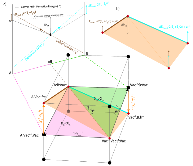
Figure 11: Mapping the composition and formation energy from a model convex hull (A-AB-B) to the constitutional space of a three-sublattice DEF model (A,Vac^-2)(B,Vac⁺²)(Vac,e^-,h⁺). Formation energies of the defect-free AB, defective AB with A-vacancy, and defective AB B-vacancy are represented by the black square, blue circle, and brown diamond, respectively. The defect lines for A-vacancy and B-vacancy are shown by the blue and brown lines, respectively. The defective compound contains charged defects, determined by the equilibrium Fermi level. (a) Graphic representation of the mapping between $X_{B}$ composition on the convex hull and the constitutional space ($Y$-space). The $X_{B}$ on the AB-B and A-AB sides maps into the green and pink regions of the $Y$-space, respectively. The charge neutrality plane is illustrated in orange. Lines in the $Y$-space that are physically relevant to the defect lines on the convex hull are shown in blue and brown. DEF end-members are depicted by black circles on the constitutional cube. Red marks indicate end-members directly connected to the formation energies on the convex hull. (b) Graphic representation of mapping the chemical potential and Fermi-level-independent defect energies onto DEF end-members’ Gibbs energies at the corners of the charge neutrality plane.

IV The General Recipe For Constructing Defect Energy Formalism

The general procedure for constructing a typical DEF model for neutral defects is as follows:

• Defect lines and defect formation energy projections on the convex hull: Plot the desired defective compounds on the formation energy convex hull. Each defective compound corresponds to a point on the convex hull diagram. The line connecting this point to the defect-free compound point is the defect line (see Ref. Anand et al. (2021)). Draw the $N_{d}$ non-parallel defect lines for $N_{d}$ different defects.

• DEF constitutional $Y$-space: Construct the constitutional space for the DEF model using the $N_{d}$ defect lines as the orthogonal basis. The origin represents the defect-free compound, and each basis vector corresponds to a defect line. Each axis indicates the site fraction of the corresponding defect on its host sublattice. The end-members are points with site fraction values of 0 or 1 along each axis. Note that the $N_{d}$ degrees of freedom, associated with fractions of defects (or secondary constituents), can be hosted on $N_{d}$ sublattices or fewer. For example, two defects (e.g., A-vacancy and B-antisite) can be defined on the first sublattice.

• DEF end-members’ Gibbs energy: The Gibbs energy of the origin point in the $Y$-space equals the formation energy of the defect-free compound, which also serves as the reference state for chemical energy. The Gibbs energy of other end-members, formed by translating the origin using defect line vectors, is the sum of the defect-free compound Gibbs energy and the absolute defect energy of the corresponding defects. Note that the number of independent DEF parameters equals $N_{d}$.

The general procedure for constructing a typical DEF model for charged defects is as follows:

• Identify the intrinsic Fermi level: The intrinsic Fermi level $E_{f}^{i}$ is typically identified from DFT calculations of the valence band maximum and band gap energies using the formula $E_{f}^{i}=E_{v}+E_{g}/2-kT/2\ln(\frac{N_{c}}{N_{v}})$.

• Ionic defect lines projections on the convex hull: The ionic defect lines with charge $q$ are constructed on the convex hull associated with $E_{f}^{i}$. The chemical-potential-independent defect energies projected on the convex hull are adjusted by adding $qE_{f}^{i}$ to yield the chemical-potential-Fermi-level-independent defect energies (see equations 6 and 25).

• DEF construction of atomic and auxiliary sublattices: The DEF model is decomposed into atomic and charge carrier sublattices. The origin of the constitutional space represents the defect-free compound, with each basis vector corresponding to a defect line. An additional basis axis describes the net concentration of free electrons and holes on the auxiliary sublattice. This model consists of $N_{d}+1$ degrees of freedom: $N_{d}$ for the number of ionic defects and one for the charge carriers.

• DEF end-members Gibbs energy: The Gibbs energy of end-members formed by the atomic sublattices is connected to their corresponding ionic defect energies on the convex hull using the same procedure as for neutral defects. The defect-free compound (i.e., the origin) serves as the reference state for chemical and electronic energies. Note that defect formation energies include the additional electronic work term, $q_{d}E_{f}^{i}$. The Gibbs energy of end-members on the auxiliary sublattice is connected to the intrinsic chemical potential of electrons and holes in a non-degenerate, defect-free compound. The reference chemical potentials of electrons and holes, $\mu_{e}^{0}$ and $\mu_{h}^{0}$, are added to the Gibbs energy of end-members containing free electrons and holes.

Competing Interests

All authors declare no competing financial or non-financial interests.

Appendix A Notes on DEF End-member Gibbs energy

In a recent study, we derived the DEF end-member Gibbs energy directly from DFT supercell energy calculations Adekoya and Snyder (2024). In Ref.Adekoya and Snyder (2024), end-members containing defects were defined by scaling the difference between the pristine supercell and the defective supercell to arrive at a stoichiometry containing the same composition as the end-member (see Eq. 12 in Ref.Adekoya and Snyder (2024)). In this section, we show that the general derivation presented in this paper can be reformatted to arrive at the same formulation as Ref.Adekoya and Snyder (2024).

For a B-vacancy defect in A_pB_q, represented by the (A)_p(Va)_q end-member, the general derivation presented in this paper gives the Gibbs energy as (see equation 13)

$${}^{0}G_{\text{A:Vac}}={}^{0}G_{\text{A:B}}+q\Delta E_{\text{B-vac}}=p\mu_{A}^{0}+q\mu_{B}^{0}+(p+q)\Delta H^{\text{p}}_{\text{f}}+qE_{\text{def}}-qE_{\text{prinstine}}$$

Reformatting the supercell total energy by the formation energy defined in equation 4 results in $\frac{E_{\text{prinstine}}}{l}=(p+q)\Delta H^{\text{p}}_{\text{f}}+p\mu_{A}^{0}+q\mu_{B}^{0}$. Substituting this equality gives the end-member Gibbs energy as

$${}^{0}G_{\text{A:Vac}}={}^{0}G_{\text{A:B}}+\Delta E_{\text{B-vac}}=\frac{E_{\text{prinstine}}}{l}+qE_{\text{def}}-qE_{\text{prinstine}}=qE_{\text{def}}-\frac{ql-1}{l}E_{\text{prinstine}}$$

Eq. 12 in Ref.Adekoya and Snyder (2024) presents the above equation for $q=1$ and $l=32$.

Similarly, for an A-interstitial defect represented by the (A)_p(B)_q(Aⁱ)_m end-member, we can reformat the end-member Gibbs energy of equation II.3 in terms of total supercell energies of defective and pristine compounds as the following

$${}^{0}G_{\text{A:B:A}}={}^{0}G_{\text{A:B:Vac}}+m\Delta E_{\text{A-interstitial}}=\frac{E_{\text{prinstine}}}{l}+mE_{\text{def}}-mE_{\text{prinstine}}=mE_{\text{def}}-\frac{ml-1}{l}E_{\text{prinstine}}$$

Appendix B (A,Vac)(B,Vac)(Vacⁱ,Bⁱ) Model

References

- Pei et al. (2011) Y. Pei, X. Shi, A. LaLonde, H. Wang, L. Chen, and G. J. Snyder, Nature 473, 66 (2011).
- Jood et al. (2020) P. Jood, J. P. Male, S. Anand, Y. Matsushita, Y. Takagiwa, M. G. Kanatzidis, G. J. Snyder, and M. Ohta, Journal of the American Chemical Society 142, 15464 (2020), pMID: 32786772, https://doi.org/10.1021/jacs.0c07067 .
- Seebauer and Kratzer (2006) E. G. Seebauer and M. C. Kratzer, Materials Science and Engineering: R: Reports 55, 57 (2006).
- Zheng et al. (2021) Y. Zheng, T. J. Slade, L. Hu, X. Y. Tan, Y. Luo, Z.-Z. Luo, J. Xu, Q. Yan, and M. G. Kanatzidis, Chem. Soc. Rev. 50, 9022 (2021).
- Slade et al. (2021) T. J. Slade, S. Anand, M. Wood, J. P. Male, K. Imasato, D. Cheikh, M. M. Al Malki, M. T. Agne, K. J. Griffith, S. K. Bux, C. Wolverton, M. G. Kanatzidis, and G. J. Snyder, Joule 5, 1168 (2021).
- Jiang et al. (2014) G. Jiang, J. He, T. Zhu, C. Fu, X. Liu, L. Hu, and X. Zhao, Advanced Functional Materials 24, 3776 (2014), https://onlinelibrary.wiley.com/doi/pdf/10.1002/adfm.201400123 .
- Ganose et al. (2022) A. M. Ganose, D. O. Scanlon, A. Walsh, and R. L. Z. Hoye, Nature Communications 13, 4715 (2022).
- Huang et al. (2018) Y. Huang, W.-J. Yin, and Y. He, The Journal of Physical Chemistry C 122, 1345 (2018), https://doi.org/10.1021/acs.jpcc.7b10045 .
- Park et al. (2018) J. S. Park, S. Kim, Z. Xie, and A. Walsh, Nature Reviews Materials 3, 194 (2018).
- Vidal et al. (2012) J. Vidal, S. Lany, M. d’Avezac, A. Zunger, A. Zakutayev, J. Francis, and J. Tate, Applied Physics Letters 100, 032104 (2012), https://doi.org/10.1063/1.3675880 .
- Geisz and Friedman (2002) J. F. Geisz and D. J. Friedman, Semiconductor Science and Technology 17, 769 (2002).
- Tongay et al. (2013) S. Tongay, J. Suh, C. Ataca, W. Fan, A. Luce, J. S. Kang, J. Liu, C. Ko, R. Raghunathanan, J. Zhou, F. Ogletree, J. Li, J. C. Grossman, and J. Wu, Scientific Reports 3, 2657 (2013).
- Mora-Seró (2020) I. Mora-Seró, Nature Energy 5, 363 (2020).
- Park and Walsh (2019) J.-S. Park and A. Walsh, Nature Energy 4, 95 (2019).
- Walsh and Zunger (2017) A. Walsh and A. Zunger, Nature Materials 16, 964 (2017).
- G. Pacchioni (85 0) D. L. G. G. Pacchioni, L. Skuja, Defects in \ceSiO2 and Related Dielectrics: Science and Technology (Springer Dordrecht, 2012, ISBN 978-0-7923-6685-0).
- Raghavachari et al. (2002) K. Raghavachari, D. Ricci, and G. Pacchioni, The Journal of Chemical Physics 116, 825 (2002), https://doi.org/10.1063/1.1423664 .
- Mills (1980) D. L. Mills, Journal of Applied Physics 51, 5864 (1980), https://doi.org/10.1063/1.327548 .
- Ma and Rohlfing (2008) Y. Ma and M. Rohlfing, Phys. Rev. B 77, 115118 (2008).
- Girard et al. (2019) S. Girard, A. Alessi, N. Richard, L. Martin-Samos, V. De Michele, L. Giacomazzi, S. Agnello, D. D. Francesca, A. Morana, B. Winkler, I. Reghioua, P. Paillet, M. Cannas, T. Robin, A. Boukenter, and Y. Ouerdane, Reviews in Physics 4, 100032 (2019).
- Bourrellier et al. (2016) R. Bourrellier, S. Meuret, A. Tararan, O. Stéphan, M. Kociak, L. H. G. Tizei, and A. Zobelli, Nano Letters 16, 4317 (2016), pMID: 27299915, https://doi.org/10.1021/acs.nanolett.6b01368 .
- Tuller and Bishop (2011) H. L. Tuller and S. R. Bishop, Annual Review of Materials Research 41, 369 (2011), https://doi.org/10.1146/annurev-matsci-062910-100442 .
- Brecher et al. (1990) C. Brecher, G. C. Wei, and W. H. Rhodes, Journal of the American Ceramic Society 73, 1473 (1990), https://ceramics.onlinelibrary.wiley.com/doi/pdf/10.1111/j.1151-2916.1990.tb09784.x .
- Tuller (2003) H. L. Tuller, Electrochimica Acta 48, 2879 (2003), electrochemistry in Molecular and Microscopic Dimensions.
- Aidhy et al. (2015) D. S. Aidhy, R. Sachan, E. Zarkadoula, O. Pakarinen, M. F. Chisholm, Y. Zhang, and W. J. Weber, Scientific Reports 5, 16297 (2015).
- Zhang et al. (2020) Y. Zhang, L. Tao, C. Xie, D. Wang, Y. Zou, R. Chen, Y. Wang, C. Jia, and S. Wang, Advanced Materials 32, 1905923 (2020), https://onlinelibrary.wiley.com/doi/pdf/10.1002/adma.201905923 .
- Li et al. (2019) P. Li, F. Hussain, P. Cui, Z. Li, and J. Yang, Phys. Rev. Mater. 3, 115402 (2019).
- Defferriere et al. (2021) T. Defferriere, D. Kalaev, J. L. M. Rupp, and H. L. Tuller, Advanced Functional Materials 31, 2005640 (2021), https://onlinelibrary.wiley.com/doi/pdf/10.1002/adfm.202005640 .
- Li et al. (2020) J. Li, C. Shu, A. Hu, Z. Ran, M. Li, R. Zheng, and J. Long, Chemical Engineering Journal 381, 122678 (2020).
- Marrocchelli et al. (2012) D. Marrocchelli, S. R. Bishop, H. L. Tuller, and B. Yildiz, Advanced Functional Materials 22, 1958 (2012), https://onlinelibrary.wiley.com/doi/pdf/10.1002/adfm.201102648 .
- Noureldine et al. (2015) D. Noureldine, S. Lardhi, A. Ziani, M. Harb, L. Cavallo, and K. Takanabe, J. Mater. Chem. C 3, 12032 (2015).
- Boehm et al. (2005) E. Boehm, J.-M. Bassat, P. Dordor, F. Mauvy, J.-C. Grenier, and P. Stevens, Solid State Ionics 176, 2717 (2005).
- Rogal et al. (2014) J. Rogal, S. Divinski, M. Finnis, A. Glensk, J. Neugebauer, J. Perepezko, S. Schuwalow, M. Sluiter, and B. Sundman, Physica Status Solidi. B: Basic Research 251, 97 (2014), harvest NEO Article first published online: 27 12 2013.
- Anand et al. (2022) S. Anand, M. Y. Toriyama, C. Wolverton, S. M. Haile, and G. J. Snyder, Accounts of Materials Research 3, 685 (2022), https://doi.org/10.1021/accountsmr.2c00044 .
- Toriyama et al. (2022) M. Y. Toriyama, M. K. Brod, and G. J. Snyder, ChemNanoMat 8, e202200222 (2022), https://onlinelibrary.wiley.com/doi/pdf/10.1002/cnma.202200222 .
- Freysoldt et al. (2014) C. Freysoldt, B. Grabowski, T. Hickel, J. Neugebauer, G. Kresse, A. Janotti, and C. G. Van de Walle, Rev. Mod. Phys. 86, 253 (2014).
- Hine et al. (2009) N. D. M. Hine, K. Frensch, W. M. C. Foulkes, and M. W. Finnis, Phys. Rev. B 79, 024112 (2009).
- Ramprasad et al. (2012) R. Ramprasad, H. Zhu, P. Rinke, and M. Scheffler, Phys. Rev. Lett. 108, 066404 (2012).
- Lany and Zunger (2008) S. Lany and A. Zunger, Phys. Rev. B 78, 235104 (2008).
- Lany and Zunger (2010) S. Lany and A. Zunger, Phys. Rev. B 81, 113201 (2010).
- Lany and Zunger (2009) S. Lany and A. Zunger, Modelling and Simulation in Materials Science and Engineering 17, 084002 (2009).
- Kattner (2016) U. R. Kattner, “THE CALPHAD METHOD AND ITS ROLE IN MATERIAL AND PROCESS DEVELOPMENT,” https://tecnologiammm.com.br/doi/10.4322/2176-1523.1059 (2016).
- Kattner (1997) U. R. Kattner, JOM 49, 14 (1997).
- Hickel et al. (2014) T. Hickel, U. R. Kattner, and S. G. Fries, physica status solidi (b) 251, 9 (2014), https://onlinelibrary.wiley.com/doi/pdf/10.1002/pssb.201470107 .
- Campbell et al. (2014) C. E. Campbell, U. R. Kattner, and Z.-K. Liu, Integrating Materials and Manufacturing Innovation 3, 158 (2014).
- Liu and Wang (2016) Z.-K. Liu and Y. Wang, Computational Thermodynamics of Materials (Cambridge University Press, 2016).
- Sundman et al. (2018) B. Sundman, Q. Chen, and Y. Du, Journal of Phase Equilibria and Diffusion 39, 678 (2018).
- van de Walle et al. (2017) A. van de Walle, R. Sun, Q.-J. Hong, and S. Kadkhodaei, Calphad 58, 70 (2017).
- Liu (2009) Z.-K. Liu, Journal of Phase Equilibria and Diffusion 30, 517 (2009).
- Bajaj et al. (2011) S. Bajaj, A. Landa, P. Söderlind, P. E. Turchi, and R. Arróyave, Journal of Nuclear Materials 419, 177 (2011).
- Li et al. (2021) X. Li, Z. Li, C. Chen, Z. Ren, C. Wang, X. Liu, Q. Zhang, and S. Chen, J. Mater. Chem. A 9, 6634 (2021).
- van de Walle (2013) A. van de Walle, JOM 65, 1523 (2013).
- van de Walle et al. (2018) A. van de Walle, C. Nataraj, and Z. kui Liu, Calphad (2018).
- Hillert and Staffansson (1970) M. Hillert and L. Staffansson, Acta chem. scand. 24, 3618 (1970).
- Harvig et al. (1971) H. Harvig, L. Kullberg, I. Roti, H. Okinaka, K. Kosuge, and S. Kachi, Acta Chemica Scandinavica 25, 3199 (1971).
- Sundman and Ågren (1981) B. Sundman and J. Ågren, Journal of Physics and Chemistry of Solids 42, 297 (1981).
- Andersson et al. (1986) J.-O. Andersson, A. F. Guillermet, M. Hillert, B. Jansson, and B. Sundman, Acta metallurgica 34, 437 (1986).
- Hillert (2001) M. Hillert, Journal of Alloys and Compounds 320, 161 (2001).
- Frisk and Selleby (2001) K. Frisk and M. Selleby, Journal of Alloys and Compounds 320, 177 (2001), materials Constitution and Thermochemistry. Examples of Methods, Measurements and Applications. In Memoriam Alan Prince.
- Oates et al. (1995) W. Oates, G. Eriksson, and H. Wenzl, Journal of Alloys and Compounds 220, 48 (1995), proceedings of the 5th International Meeting on Thermodynamics of Alloys.
- Chen et al. (1998) Q. Chen, M. Hillert, B. Sundman, W. A. Oates, S. G. Fries, and R. Schmid-Fetzer, Journal of Electronic Materials 27, 961 (1998).
- Li and Kerr (2013) J. Li and L. L. Kerr, Optical Materials 35, 1213 (2013).
- Hu et al. (2018) Y. Hu, J. Paz Soldan Palma, Y. Wang, S. Firdosy, K. Star, J. Fleurial, V. Ravi, and Z. Liu, Calphad: Computer Coupling of Phase Diagrams and Thermochemistry 61, 227 (2018).
- Peters et al. (2019) M. C. Peters, J. W. Doak, J. E. Saal, G. B. Olson, and P. W. Voorhees, Journal of Electronic Materials 48, 1031 (2019).
- Peters et al. (2017) M. Peters, J. Doak, W.-W. Zhang, J. Saal, G. Olson, and P. Voorhees, Calphad 58, 17 (2017).
- Bajaj et al. (2015) S. Bajaj, G. S. Pomrehn, J. W. Doak, W. Gierlotka, H. jay Wu, S.-W. Chen, C. Wolverton, W. A. Goddard, and G. Jeffrey Snyder, Acta Materialia 92, 72 (2015).
- Chen and Hillert (1996) Q. Chen and M. Hillert, Journal of Alloys and Compounds 245, 125 (1996).
- Sundman et al. (2011) B. Sundman, C. Guéneau, and N. Dupin, Acta Materialia 59, 6039 (2011).
- Guan et al. (2017) P.-W. Guan, S.-L. Shang, G. Lindwall, T. Anderson, and Z.-K. Liu, Calphad 59, 171 (2017).
- Anand et al. (2021) S. Anand, J. P. Male, C. Wolverton, and G. J. Snyder, Mater. Horiz. 8, 1966 (2021).
- Adekoya and Snyder (2024) A. H. Adekoya and G. J. Snyder, Advanced Functional Materials , 2403926 (2024), https://onlinelibrary.wiley.com/doi/pdf/10.1002/adfm.202403926 .
- Sze and Ng (2006) S. Sze and K. . Ng, “Physics and properties of semiconductors—a review,” in Physics of Semiconductor Devices (John Wiley & Sons, Ltd, 2006) pp. 5–75, https://onlinelibrary.wiley.com/doi/pdf/10.1002/9780470068328.ch1 .
- See (2009) “Fundamentals of defect ionization and transport,” in Charged Semiconductor Defects: Structure, Thermodynamics and Diffusion (Springer London, London, 2009) pp. 5–37.