Information-Theoretic Foundations for Machine Learning

Abstract

The staggering progress of machine learning over the past decade has been a sight to behold. In retrospect, it is both remarkable and unsettling that these milestones were achievable with little to no rigorous theory to guide experimentation. Despite this fact, practitioners have been able to guide their future experimentation via observations from previous large-scale empirical investigations. However, alluding to Plato’s Allegory of the cave, it is likely that the observations which form the field’s notion of reality are but shadows representing fragments of that reality. In this work, we propose a theoretical framework which attempts to answer what exists outside of the cave. To the theorist, we provide a framework which is mathematically rigorous and leaves open many interesting ideas for future exploration. To the practitioner, we provide a framework whose results are very intuitive, general, and which will help form principles to guide future investigations. Concretely, we provide a theoretical framework rooted in Bayesian statistics and Shannon’s information theory which is general enough to unify the analysis of many phenomena in machine learning. Our framework characterizes the performance of an optimal Bayesian learner, which considers the fundamental limits of information. Unlike existing analyses that weaken with increasing data complexity, our theoretical tools provide accurate insights across diverse machine learning settings. Throughout this work, we derive very general theoretical results and apply them to derive insights specific to settings ranging from data which is independently and identically distributed under an unknown distribution, to data which is sequential, to data which exhibits hierarchical structure amenable to meta-learning. We conclude with a section dedicated to characterizing the performance of misspecified algorithms. These results are exciting and particularly relevant as we strive to overcome increasingly difficult machine learning challenges in this endlessly complex world.

1 Introduction

In the past decade, the staggering progress of machine learning has been a sight to behold. The research community has conquered games such as go, which were thought to require human-level learning and abstraction capabilities [Silver et al., 2016]. We have produced systems which are capable of displaying common-sense and holding coherent dialogues with humans around the globe [Achiam et al., 2023]. It is undeniable that these artifacts will be remembered throughout the future of humanity’s pursuit of discovering and understanding intelligence.

In retrospect, it is both remarkable and unsettling that these milestones were achievable with little to no rigorous theory to guide experimentation. While theorists have attempted to repurpose existing statistical tools to analyze modern machine learning, the conclusions have largely contradicted the observations of practitioners. Zhang et al. [2021] aptly demonstrated this point via a series of simple experiments which elucidated the fundamental incompatibility of empirically observed phenomena with existing notions of generalization. Despite this incoherence, practitioners have been able to guide their future experimentation based on prior large-scale empirical investigations. However, without a clear idea of how these phenomena slot into a larger picture, many research efforts will continue to be led astray. Alluding to Plato’s Allegory of the cave, it is likely that the observations which form the field’s notion of reality are but shadows representing fragments of that reality.

In this work, we propose a theoretical framework which attempts to answer what exists outside of the cave. To the theorist, we provide a framework which is mathematically rigorous and leaves open many interesting ideas for future exploration. To the practitioner, we provide a framework whose results are very intuitive, general, and which will help form principles to guide future investigations. Concretely, we provide a theoretical framework rooted in Bayesian statistics which is general enough to unify the analysis of many phenomena in machine learning.

Our theoretical framework draws inspiration from both Shannon’s theory of information and his maxim of “information first, then computation”. The turn of the twentieth century brought a wave of interest in communications research; work that would enable the transmission of signals across long distances. Much of the work in encoding/decoding was approached heuristically, similarly to how deep learning is today. Shannon’s theory and maxim redirected attention to characterizing what was fundamentally possible or impossible, in the absence of computational constraints. His theory guided the discovery of algorithms which achieved these fundamental limits and eventually practical implementations as well.

The aforementioned staggering feats of machine learning and artificial intelligence have fueled optimism that anything is learnable with sufficient data and computation. However, research directions have largely been informed by informal reasoning supported by a plethora of empirical studies. While work in statistics provides some guidance, the results for the most part lack the generality required to explain the continuing onslaught of novel empirical findings. This monograph aims to provide a general framework to elucidate what is possible by studying how the limits of performance in machine learning depend on the informational content of the data. Our framework is based on Shannon’s information theory and characterizes the dependence of performance on information in the absence of computational constraints. Concretely, we characterize the performance of an optimal Bayesian learner that observes data generated by a suite of data generating processes of increasing complexity. By expressing what is fundamentally possible in machine learning, we aim to develop intuition that can guide fruitful investigation.

Our framework characterizes the performance of an optimal Bayesian learner, which considers the fundamental limits of information. Unlike existing analyses that weaken with increasing data complexity, our theoretical tools provide accurate insights across diverse machine learning settings. For example, previous theories about learning from sequential data rely on specific and rigid mixing time assumptions. However, Jeon et al. [2024] leverage our framework to arrive at more general results which characterize the sample complexity of learning from sequences autoregressively generated by transformers [Vaswani et al., 2017]. They further extend the techniques to analyze hierarchical data generating processes which resemble meta-learning and in-context learning in large language models (LLMs). That these analytic techniques remarkably apply whether data is exchangeable or exhibits more complex structure points to the fundamental nature of our findings.

In recent years, we have observed that training larger machine learning models on more data continues to produce significantly better performance. This continual improvement indicates that the data generating processes that we study are more complex than the machine learning models which we fit. We refer to this phenomenon as “misspecification” and it is prominently observed in natural language processing (NLP), where researchers have tried to mathematically characterize this improvement in performance [Kaplan et al., 2020, Hoffmann et al., 2022]. The “neural scaling laws” of Kaplan et al. [2020] and Hoffmann et al. [2022] characterize the rate at which out-of-sample log-loss decreased with respect to more available compute and data. While these works provide extensive empirical experimentation, their cursory mathematical analysis leave open many questions regarding how scaling laws change depending on the complexity of the data-generating process. Jeon and Roy [2024] once again use the theoretical tools from this monograph to rigorously characterize the error incurred by a misspecified algorithm. They study a data-generating process which is identified by an single hidden-layer network of infinite width and characterize how an algorithm with finite budget should optimally allocate between parameter count and dataset size. These results notably are consistent (up to logarithmic factors) with the the findings of Hoffmann et al. [2022], where the optimal dataset size and parameter count exhibit a linear relationship.

Despite the fact that our theory does not address computational constraints, empirical studies with neural networks suggest that practical stochastic gradient algorithms suffice to attain the tradeoffs that our theory establishes between information and performance [Zhu et al., 2022]. Throughout this work, we derive very general theoretical results and apply them to derive insights specific to settings ranging from data which is iid under an unknown distribution to data which is sequential to data which exhibits hierarchical structure amenable to meta-learning. We conclude with a section dedicated to characterizing the performance of suboptimal algorithms that are based on misspecified models, an exciting and relevant direction for future work.

2 Related Works

2.1 Frequentist and Bayesian Statistics

We begin with a discussion of frequentist statistics, the predominant framework which encompasses existing theoretical results. As its name would suggest, in frequentist statistics, probability describes how often an event occurs if a procedure is repeated many times. For instance, suppose there exists an unknown parameter $\mu\in\Re$ and a sample of size $T$: $(X_{1},X_{2},\ldots,X_{T})$ which is drawn iid $\mathcal{N}(\mu,1)$. After observing the sample, the frequentist statistician may construct a $95\%$ confidence interval for the unknown $\mu$. However, recall that in frequentism, probability is assigned to how often an event occurs if a procedure is repeated many times. For our example, this entails that if random samples of size $T$ were drawn repeatedly and their corresponding confidence intervals constructed, then $95\%$ of those confidence intervals would contain $\mu$. Note that the unknown parameter $\mu$ is fixed and hence not a random variable in the frequentist framework. As a result, the frequentist framework does not use the tools of probability to model uncertainty pertaining to $\mu$.

In contrast, Bayesian statistics treats all unknown quantities as random variables. A consequence is that these quantities must be assigned subjective probabilities which reflect one’s prior beliefs pertaining to their values. Returning to our example, the Bayesian may assign a prior distribution $\mathbb{P}(\mu\in\cdot)=\mathcal{N}(0,1)$ which reflects their beliefs prior to observing the sample. After observing the sample $(x_{1},x_{2},\ldots,x_{T})$, they may construct a 95% credible interval for $\mu$, an interval $(a,b)$ for which $\mathbb{P}(\mu\in(a,b)|X_{1}=x_{1},X_{2}=x_{2},\ldots,X_{T}=x_{T})\geq 0.95$. The posterior distribution $\mathbb{P}(\mu\in\cdot|X_{1}=x_{1},X_{2}=x_{2},\ldots,X_{T}=x_{T})$ is computed via Bayes rule. Note that unlike the frequentist confidence interval which pertains to repeated experimentation, the Bayesian credible interval states that for this particular sample, with 95% probability, $\mu\in(a,b)$. However, we note that this probability is subjective as it relies upon the prior subjective probability $\mathbb{P}(\theta\in\cdot)$. While this subjectivism has been a topic of constant philosophical debate, we note that in the realm of decision theory, it is well known that the choices of a decision maker which abides by axioms of rationality can be explained as the result of a utility function and subjective probabilities assigned to events [Savage, 1972].

While the debate surrounding these two schools of thought have continued for almost a century, it is prudent to consider the purpose for such theory. We are reminded of Laplace’s prudent remark that “Probability theory is nothing but common sense reduced to calculation”. Theory’s merit ought to stem from the results it can provide for specific problems [Jaynes and Kempthorne, 1976]. Jaynes and Kempthorne [1976] espoused this viewpoint as their background in physics led to their interest in the use of probability to describe and predict phenomena of the physical world. Machine learning too is is rooted in predictions based on data produced by the physical world. Therefore, we argue that the merits of machine learning theory also ought to stem from its ability to describe and predict phenomena of data generated by the physical world. To this end, we believe that the results which we derive via our framework both better reflect what is observed empirically and are also general enough to unify many disparate areas of the field.

2.2 PAC Learning

The majority of existing theoretical results for the analysis of modern machine learning are set in the probably approximately correct (PAC) learning framework [Valiant, 1984]. In PAC learning, an algorithm is presented with a sample of data and is tasked with returning a hypothesis from a hypothesis set which can accurately perform predictions out-of-sample. The probably approximately correct come from the detail that these results are phrased as follows: “For any data distribution, with probability at least $1-\delta$ over the randomness of an iid sample, the excess out-of-sample error is $\leq\epsilon$”. “Probably” refers to the $1-\delta$ probability and “approximately correct” the $\epsilon$ tolerance of out-of-sample error. While this framework has facilitated the development of influential theoretical concepts such as VC dimension [Vapnik, 2013] and Rademacher complexity [Bartlett and Mendelson, 2002], Zhang et al. [2021] have demonstrated that these tools are inherently insufficient to explain modern empirical phenomena. Namely, they demonstrate empirically that while the Rademacher complexity of a deep neural networks leads to vacuous theoretical results, the observed out-of-sample error of these deep neural networks is actually small.

We posit that the looseness of these theoretical results stems from the fact that they hold for any data distribution and uniformly over the hypothesis set. While it is true that Rademacher complexity depends on the distribution of the inputs, it does not depend on the joint distribution of the input and outputs. Meanwhile, data which we observe from the real world clearly contains inherent structure between input and output which facilitate sample-efficient learning. Suppose we perform binary classification with input $X\sim\mathcal{N}(0,I_{d})$. In case $1$, consider a data generating process in which the corresponding class $Y$ only depends on the first element of $X$. In case $2$, consider a data generating process in which $Y$ depends on all $d$ elements of $X$. Common sense would dictate that if we observed an equal number of samples from each data generating process and considered the same hypothesis spaces, the generalization error of case $1$ ought to be lower than that of case $2$. However, an analysis via VC dimension or Rademacher complexity would result in the same generalization bound for case $1$ and $2$. This problem exacerbated by high dimensional input distributions and overparameterized hypothesis classes, both of which are prevalent qualities of deep learning.

Several lines of analysis have attempted to ameliorate this via data dependent bounds. While these results also hold for any data distribution, the choice of data distribution will impact the resulting error bound. Therefore, such a result will be vacuous (as expected) for a problem instance with unstructured data, but potentially much tighter for one which exhibits structure. The main frameworks for data dependent PAC results involve PAC Bayes [McAllester, 1998] and the information-theoretic framework of Xu and Raginsky [2017]. Both frameworks involve an algorithm which produces a predictive distribution of the hypothesis conditioned on the observed data (hence they analyze a Bayesian algorithm under the PAC framework). The two only differ in that PAC Bayes results hold with high probability over random draws of the data while the information-theoretic results hold in expectation over random draws of the data. Therefore, each result upper bounds generalization error via the KL divergence or the mutual information between the observed data and the hypothesis.

These data dependent results mark a significant step in understanding the puzzling empirical success of deep learning. Notably, Dziugaite and Roy [2017] establish PAC-Bayes results for deep neural networks which result in bounds that dramatically improve upon those based on parameter count or VC dimension. These results reflect the importance that the data generating process has on the generalization error. However, a limitation is the lack of theoretical tools which facilitate analytic derivations. Namely, the aforementioned KL divergence/mutual information which bound generalization cannot be computed analytically outside of simple problem instances. This is because these quantities involve the posterior distribution of the hypothesis conditioned on the data, which cannot be expressed analytically outside of simple instances which exhibit a conjugate distribution. In contrast, our results analyze these quantities in a Bayesian setting, allowing us to develop general tools to bound mutual information analytically without needing to write down these complicated posterior distributions. The conciseness and generality of these results lead us to believe that they are fundamental.

2.3 Information Theory

The results of this work elucidate the tight relation between error in learning and information measures of Shannon’s theory [Shannon, 1948]. Prior work establishes connections between information theory and parameter estimation notably through information-theoretic lower bounds. Namely, the global Fano method resembles a portion of the techniques which we will cover in this monograph.

A widely known framework involving information theory and machine learning is the information bottleneck method [Tishby et al., 2000]. On the surface, this work exhibits many similarities to ours as it draws a connection between information theory, rate-distortion theory and machine learning. However, the two works diverge in their purpose. The information bottleneck framework describes a learning objective rooted in information theory and prescribes a learning algorithm to solve this optimization problem. While they leveraged their framework to produce early work on generalization in deep neural networks [Tishby and Zaslavsky, 2015], the results remained very abstract. While they devised metrics which they approximate empirically, they do not provide theoretical tools to analyze these metrics analytically. In contrast, we present our framework with a collection of theoretical tools which facilitate analytic solutions. This is an important property of a theoretical framework as it allows the researcher to forecast what ought to be possible in practice.

As alluded to above, there exist notable information-theoretic generalization results in the PAC learning framework introduced by Russo and Zou [2019] and expanded upon by Xu and Raginsky [2017]. While our work shares similar analytic techniques, we are able to strengthen the results and provide more streamlined theoretical tools by framing results in a Bayesian setting. In particular, this framing allows us to upper and lower bound the mutual information between the data and a latent parameter via the rate-distortion function, which we can characterize analytically for even complex data generating processes. We find the results of our framing to be fundamental and we hope that the readers share this sentiment. We also hope that provides the reader with a new perspective on machine learning.

The recent advances in LLMs have incited an interest in the connection between learning and compression. In particular, researchers have posited that models which are better able to compress the observed data will achieve lower out-of-sample error. This point is conveyed in [Deletang et al., 2024]. However, they do not provide a mathematically rigorous connection between learning and compression. In this work we establish a rigorous connection between learning and optimal lossy compression. The loss incurred by an optimal Bayesian learner is upper and lower bounded by appropriate expressions containing the rate-distortion function (characterization of optimal lossy compression). For this community, we hope that our work provides clarity to this matter and informs future experimentation and algorithm design.

3 A Framework for Learning

3.1 Probabilistic Framework and Notation

In our work, we define all random variables with respect to a common probability space $(\Omega,\mathbb{F},\mathbb{P})$. Recall that a random variable $\theta$ is a measurable function $\Omega\mapsto\Theta$ from the sample space $\Omega$ to a set $\Theta$.

The probability measure $\mathbb{P}:\mathbb{F}\mapsto[0,1]$ assigns probabilities to events in the $\sigma-{\rm algebra}$ $\mathbb{F}$. In particular, for any event $F\in\mathbb{F}$, $\mathbb{P}(F)$ denotes the probability of the event. For events $F,G\in\mathbb{F}$ for which $\mathbb{P}(G)>0$, $\mathbb{P}(F|G)$ denotes the probability of event $F$ conditioned on event $G$.

For each realization $z$ of a random variable $Z$, $\mathbb{P}(Z=z)$ is hence a function of $z$. We denote the value of this function evaluated at $Z$ by $\mathbb{P}(Z)$. Therefore, $\mathbb{P}(Z)$ is a random variable (since it takes realizations in $[0,1]$ depending on the value of $Z$). Likewise for realizations $(y,z)$ of random variables $Y,Z$, $\mathbb{P}(Z=z|Y=y)$ is a function of $(y,z)$ and $\mathbb{P}(Z|Y)$ is a random variable which denotes the value of this function evaluated at $(Y,Z)$.

If random variable $Z:\Omega\mapsto\Re^{K}$ has density $p_{Z}$ w.r.t the Lebesgue measure, the conditional probability $\mathbb{P}(F|Z=z)$ is well-defined despite the fact that for all $z$, $\mathbb{P}(Z=z)=0$. If function $f(z)=\mathbb{P}(F|Z=z)$ and $Y:\Omega\mapsto\Re^{K}$ is a random variable whose range is a subset of $Z$’s, then we use the $\leftarrow$ symbol with $\mathbb{P}(F|Z\leftarrow Y)$ to denote $f(Y)$. Note that this is different from $\mathbb{P}(F|Z=Y)$ since this conditions on the event $Z=Y$ while $\mathbb{P}(F|Z\leftarrow Y)$ indicates a change of measure.

For any random variable $\theta$, we use the notation $\mathbb{P}(\theta\in\cdot)$ to denote the distribution of that random variable i.e. $\mathbb{P}(\theta\in\cdot)=\mathbb{P}(\theta^{-1}(\cdot))$, where $\theta^{-1}(\cdot)$ denotes the pre-image of $\cdot$ (the pre-image must be $\in\mathbb{F}$ due to measurability). We make a clear distinction between a random variable and its distribution in this way to provide accurate definitions of information-theoretic quantities later in this work. As mentioned in the introduction, our framework is Bayesian, and hence uses the tools of probability to model uncertainty about the unknown value of a variable of interest (for instance $\theta$). This involves treating $\theta$ as a random variable with a prior distribution $\mathbb{P}(\theta\in\cdot)$ which encodes the designer’s prior information about the value of this variable. The designer will often never directly observe $\theta$, but rather a stream of data which will contain information about $\theta$. Machine Learning is therefore the process of reducing uncertainty about $\theta$ in ways that are relevant for making better predictions about the future of this data stream.

3.2 Data Generating Process

In machine learning, we are interested in discerning the relationship between input and output pairs $(X,Y)$. Most frameworks of machine learning focus on a static dataset of fixed size and hope to characterize the performance of a predictive algorithm which leverages the information from the dataset for future predictions. However, any practical system will continually have access to additional observations as it interacts with the environment. As a result, it is prudent to consider a framework in which the data arrives in an online fashion and the objective is to perform well across all time.

We consider a stochastic process which generates a sequence $((X_{t},Y_{t+1}):t\in\mathbb{Z}_{+})$ of data pairs. For all $t$, we let $H_{t}$ denote the history $(X_{0},Y_{1},\ldots,X_{t-1},Y_{t},X_{t})$ of experience. We assume that there exists an underlying latent variable $\theta$ such that $(X_{0},X_{1},\ldots)\perp\theta$ and $\theta$ prescribes a conditional probability measure $\theta(\cdot|H_{t})$ to the next label $Y_{t+1}$. In the case of an iid data generating process, this conditional probability measure would only depend on $H_{t}$ via $X_{t}$. Furthermore, such a latent variable $\theta$ must exist under an infinite exchangability assumption on the sequence $((X_{t},Y_{t+1}):t\in\mathbb{Z}_{+})$ by de Finetti’s Theorem. While we will first focus on this iid setting, we will also study learning setting in which the future data may be arbitrarily dependent on $H_{t}$ even when conditioned on $\theta$. As our framework is Bayesian, we represent our uncertainty about $\theta$ by modeling it as a random variable with prior distribution $\mathbb{P}(\theta\in\cdot)$.

3.3 Error

Our framework focuses on a particular notion of error which facilitates analysis via Shannon-information theory. For all $t\in\mathbb{Z}_{+}$, our algorithm is tasked with providing a predictive distribution $P_{t}$ of $Y_{t+1}$ which may be derived from the history of data $H_{t}$ which has already been observed. We denote such algorithm as $\pi$ for which for all $t$, $P_{t}=\pi(H_{t})$. As aforementioned, an effective learning system ought to leverage data as it becomes available. As a result, for any time horizon $T\in\mathbb{Z}_{+}$, we are interested in quantifying the cumulative expected log-loss:

$$\mathbb{L}_{T,\pi}=\frac{1}{T}\sum_{t=0}^{T-1}\mathbb{E}_{\pi}\left[-\ln P_{t}(Y_{t+1})\right].$$

As outlined in section 3.1, we take all random variables to be defined with respect to a common probability space. As a result, the expectation $\mathbb{E}$ integrates over all random variables which we do not condition on. We use the subscript $\pi$ in $\mathbb{E}_{\pi}$ to specify that it is a function of $\pi$ since for all $t$, $\pi$ produces $P_{t}$. As $Y_{t+1}$ is the random variable which represents the next label that is generated by the underlying stochastic process, $P_{t}(Y_{t+1})$ denotes the probability that our prediction $P_{t}$ assigned to label $Y_{t+1}$.

This loss function is commonly referred to in the literature as “log-loss” or “negative log-likelihood” and has become a cornerstone of classification methods via neural networks. However, it is important to note that even for an optimal algorithm, the minimum achievable log-loss is not $0$. For instance, consider an omniscient algorithm in the classification setting which produces for all $t$ the prediction $P_{t}=\mathbb{P}(Y_{t+1}\in\cdot|\theta,H_{t})$. Even this agent incurs a loss of:

$$\frac{1}{T}\sum_{t=0}^{T-1}\mathbb{E}_{\pi}\left[-\ln\mathbb{P}(Y_{t+1}|\theta,H_{t})\right] =\frac{1}{T}\sum_{t=0}^{T-1}\mathbb{H}(Y_{t+1}|\theta,H_{t})$$

$$=\frac{\mathbb{H}(Y_{1:T}|\theta,X_{0:T-1})}{T},$$

where our point follows from the fact that the conditional entropy of a discrete random variable $Y_{1:T}$ is non-negative. As a result, we define the estimation error as:

$$\mathcal{L}_{T,\pi}=\mathbb{L}_{T,\pi}-\frac{\mathbb{H}(Y_{1:T}|\theta,X_{0:T-1})}{T}.$$

Estimation error represents the error which is reducible via learning. As such, for a competent learning algorithm tasked with a learnable task, $\mathcal{L}_{T,\pi}$ should decay to $0$ as $T$ goes to $\infty$.

3.4 Achievable Error

Since we are interested in characterizing the limits of what is possible via machine learning, a natural question which arises is: For all $T$, which $\pi$ minimizes $\mathcal{L}_{T,\pi}$? Since log-loss is a proper scoring rule, the optimal algorithm $\pi$ is one such that for all $t$, $P_{t}=\mathbb{P}(Y_{t+1}\in\cdot|H_{t})$. This predictive distribution is often referred to as the Bayesian posterior and going forward we will denote it by $\hat{P}_{t}$. The following result establishes optimality of $\hat{P}_{t}$.

Lemma 1.

(Bayesian posterior is optimal) For all $t\in\mathbb{Z}_{+}$,

$$\mathbb{E}\left[-\ln\hat{P}_{t}(Y_{t+1})\mid H_{t}\right]\ \overset{a.s.}{=}\ \min_{\pi}\ \mathbb{E}_{\pi}\left[-\ln P_{t}(Y_{t+1})\mid H_{t}\right].$$

Proof.

$$\mathbb{E}\left[-\ln P_{t}(Y_{t+1})|H_{t}\right] \overset{a.s.}{=}\mathbb{E}\left[-\ln\hat{P}_{t}(Y_{t+1})+\ln\frac{\hat{P}_{t}(Y_{t+1})}{P_{t}(Y_{t+1})}\bigg{|}H_{t}\right]$$

$$\overset{a.s.}{=}\mathbb{E}\left[-\ln\hat{P}_{t}(Y_{t+1})|H_{t}\right]+{\mathbf{d}}_{\rm KL}\left(\hat{P}_{t}\|P_{t}\right).$$

The result follows from the fact that KL-divergence is non-negative and the tower property. ∎

This result is rather convenient since it prescribes that across all problem instances, the optimal prediction is $\hat{P}_{t}$. This is widely considered an advantage of the Bayesianism as opposed to the frequentism; the Bayesian need not specify an ad-hoc algorithm to analyze/solve a problem. While in practice it may be intractable to compute $\hat{P}_{t}$ exactly, for the purposes of characterizing achievable error, it provides immense utility. Going forward, we will restrict our attention to the optimal achievable estimation error which we denote by:

$$\mathcal{L}_{T}=\frac{1}{T}\sum_{t=0}^{T-1}\mathbb{E}\left[-\ln\hat{P}_{t}(Y_{t+1})\right]-\frac{\mathbb{H}(Y_{1:T}|\theta,X_{0:T-1})}{T}.$$

The process of learning should result in $\mathcal{L}_{T}$ vanishing to $0$ as $T$ increase to $\infty$. While we have established that the Bayesian posterior provides optimal predictions at each timestep, in its current form, it is unclear how to characterize $\mathcal{L}_{T}$ for problems in which the posterior distribution does not exhibit an analytic form. In section 5, we will establish the connection between our learning framework and information theory. This connection will facilitate the analysis of arbitrary learning problems, even those for which $\hat{P}_{t}$ cannot be expressed analytically.

In the following section, we overview requisite definitions and tools from information theory to establish the connection between learning and information theory. For readers who are new to information theory, we provide the following section for completeness. Even for readers who are familiar with information theory, there may be details or results is the following section which may be worth revisiting.

Summary

• The algorithm’s observations through time $t$ form a history $H_{t}=(X_{0},Y_{1},\ldots X_{t-1},Y_{t},X_{t})$.

• The algorithm $\pi$ produces for all $t$ a predictive distribution $P_{t}$ of $Y_{t+1}$ given the history $H_{t}$.

• For any horizon $T\in\mathbb{Z}_{+}$, we define estimation error of an algorithm $\pi$ as

  $$\mathcal{L}_{T,\pi}=\underbrace{\frac{1}{T}\sum_{t=0}^{T-1}\mathbb{E}_{\pi}\left[-\ln P_{t}(Y_{t+1})\right]}_{\rm log-loss}-\underbrace{\frac{\mathbb{H}(Y_{1:T}|\theta,X_{0:T-1})}{T}}_{\rm irreducible\ error}.$$

• The optimal algorithm assigns for all $t$,

  $$P_{t}\leftarrow\hat{P}_{t}=\mathbb{P}(Y_{t+1}\in\cdot|H_{t}).$$

• We denote the estimation error incurred by the optimal algorithm by

  $$\mathcal{L}_{T}=\frac{1}{T}\sum_{t=0}^{T-1}\mathbb{E}_{\pi}\left[-\ln\hat{P}_{t}(Y_{t+1})\right]-\frac{\mathbb{H}(Y_{1:T}|\theta,X_{0:T-1})}{T}.$$

4 Requisite Information Theory

In this section we outline definitions and results from information theory which we will refer to in later sections of this monograph. For a comprehensive overview of the topic, we point the reader to [Cover and Thomas, 2012].

4.1 Entropy

In this text, $\mathbb{H}(X)$ denotes the entropy of a discrete random variable $X:\Omega\mapsto\mathcal{X}$. $\mathbb{H}$ is defined as follows:

$$\mathbb{H}(X)=\sum_{x\in\mathcal{X}}\mathbb{P}(X=x)\ln\frac{1}{\mathbb{P}(X=x)}.$$

Throughout this monograph, we use the convention that $0\ln 0=0$. While there are many colloquial interpretations of entropy which describe it as the expected “surprise” associated with outcomes of a random variable, we provide a concrete motivation for entropy based on coding theory.

We begin our exposition of entropy with an introduction to coding theory. We first define a code for a random variable.

Definition 2.

A code $C$ for random variable $X:\Omega\mapsto\mathcal{X}$ is a function which maps $\mathcal{X}\mapsto\{0,1\}^{*}$, where $\{0,1\}^{*}$ denotes the set of all binary strings.

When we send a text message to our friend, the characters that comprise of our message can be thought of as the realizations of random variables. In many applications involving digital data transfer, a message (outcome of a random variable) is encoded into a binary string which is passed through a communication channel, and decoded at an endpoint. Since the binary string arrives in a stream, it would be convenient if the message could be uniquely decoded as the data is arriving. A necessary and sufficient condition for this is online decodability is to design a code $C$ which is prefix-free i.e. no element in the image of $C$ is a prefix of another element in the image of $C$. We use $\mathcal{C}_{X}$ to denote the set of prefix-free codes for a random variable $X$

Since these codes are stored, transmitted, and decoded, the memory footprint becomes a significant design consideration. A natural question which arises is: “how do we devise optimal prefix-free codes?” The notion of optimality which gives rise to Shannon entropy is the following:

$$\operatorname*{arg\,min}_{C\in\mathcal{C}_{X}}\ \sum_{x\in\mathcal{X}}\mathbb{P}(X=x)\cdot\frac{\text{len}\left(C(x)\right)}{\log_{2}(e)},$$

where $\text{len}(c)$ denotes the length of binary string $c$. A prefix-free code which minimizes this objective will on-average require the fewest number of bits to store/transmit information. A naive prefix-free code is one which maps each of the $|\mathcal{X}|$ outcomes of $X$ to a unique binary string of length $\lceil\log_{2}|\mathcal{X}|\rceil$. While such a code would be reasonable if all outcomes of $X$ were equally likely, such a code would be highly suboptimal if some outcomes are much more/less likely than others. A competent coding scheme ought to map more likely outcomes to shorter strings and less likely outcomes to longer strings.

Figure 1: The English alphabet consists of characters of varying frequency across common text corpuses. Notably, the vowels appear with greater frequency. A coding scheme ought to map these more frequently appearing characters to shorter strings.

The following result establishes the tight connection between the entropy of $X$ and its optimal prefix-free code.

Theorem 3.

(entropy characterizes optimal prefix-free code length) For all discrete random variables $X:\Omega\mapsto\mathcal{X}$,

$$\mathbb{H}(X)\ \leq\ \min_{C\in\mathcal{C}_{X}}\ \sum_{x\in\mathcal{X}}\mathbb{P}(X=x)\cdot\frac{{\rm len}(C(x))}{\log_{2}(e)}\ \leq\ \mathbb{H}(X)+\frac{1}{\log_{2}(e)}.$$

This result demonstrates that the entropy of a random variable tightly characterizes the fundamental limit to which it can be losslessly compressed. As a result, the entropy reflects the inherent complexity of a random variable. This connection is useful to keep in mind as there exist the following analogies between our Bayesian and the frequentist frameworks:

frequentist $$\mapsto\text{Bayesian}$$

$$\Theta \mapsto\mathbb{P}(\theta\in\cdot)$$

$$|\Theta| \mapsto\mathbb{H}(\theta),$$

where $\theta:\Omega\mapsto\Theta$ and $|\Theta|$ denotes the cardinality of $\Theta$.

4.2 Conditional Entropy

$\mathbb{H}(X|Y)$ denotes the conditional entropy of a discrete random variable $X:\Omega\mapsto\mathcal{X}$ conditioned on another discrete random variable $Y:\Omega\mapsto\mathcal{Y}$. The conditional entropy is defined as follows:

$$\mathbb{H}(X|Y)=\sum_{x\in\mathcal{X},y\in\mathcal{Y}}\mathbb{P}(X=x,Y=y)\ln\frac{1}{\mathbb{P}(X=x|Y=y)}.$$

Note that unlike conditional expectation, conditional entropy is a number (and not a random variable). Upon closer inspection it is clear that conditional entropy is also always non-negative and is $0$ only when $Y$ fully determines $X$. On the other hand, when $X\perp Y$, we have that $\mathbb{H}(X|Y)=\mathbb{H}(X)$. We provide the following result which facilitates mathematical manipulations involving the information-theoretic quantities outlined thus far.

Lemma 4.

(chain rule of conditional entropy) For all discrete random variables $X:\Omega\mapsto\mathcal{X},Y:\Omega\mapsto\mathcal{Y}$,

$$\mathbb{H}(X,Y)\ =\ \mathbb{H}(X)+\mathbb{H}(Y|X)\ =\ \mathbb{H}(Y)+\mathbb{H}(X|Y).$$

Proof.

$$\mathbb{H}(X)+\mathbb{H}(Y|X) =\sum_{x\in\mathcal{X}}\mathbb{P}(X=x)\ln\frac{1}{\mathbb{P}(X=x)}+\sum_{x\in\mathcal{X},y\in\mathcal{Y}}\mathbb{P}(X=x,Y=y)\ln\frac{1}{\mathbb{P}(Y=y|X=x)}$$

$$=\sum_{x\in\mathcal{X},y\in\mathcal{Y}}\mathbb{P}(X=x,Y=y)\ln\frac{1}{\mathbb{P}(X=x)}+\sum_{x\in\mathcal{X},y\in\mathcal{Y}}\mathbb{P}(X=x,Y=y)\ln\frac{\mathbb{P}(X=x)}{\mathbb{P}(X=x,Y=y)}$$

$$=\sum_{x\in\mathcal{X},y\in\mathcal{Y}}\mathbb{P}(X=x,Y=y)\ln\frac{1}{\mathbb{P}(X=x,Y=y)}$$

$$=\mathbb{H}(X,Y).$$

The second equality in the lemma statement follows from the same technique shown above. ∎

If $\mathbb{H}(X,Y)$ denotes the average length of a prefix-free code for $(X,Y)$ jointly, Lemma 4 establishes that $\mathbb{H}(X|Y)$ reflects the average length of a prefix-free code for $X$ after $Y$ is already observed. Evidently if $X\perp Y$, then observing $Y$ does not provide any information which enables a shorter code for $X$ (hence, $\mathbb{H}(X|Y)=\mathbb{H}(X)$). However, in the other extreme in which $X\overset{a.s.}{=}Y$, observing $Y$ means that $X$ is also known. As a result, a trivial code which maps every outcome of $X$ to the null string $\emptyset$ will suffice (hence, $\mathbb{H}(X|Y)=0$).

4.3 Mutual Information

$\mathbb{I}(X;Y)$ denotes the mutual information between two random variables $X:\Omega\mapsto\mathcal{X}$ and $Y:\Omega\mapsto\mathcal{Y}$. Concretely,

$$\mathbb{I}(X;Y)\ =\ {\mathbf{d}}_{\rm KL}\left(\mathbb{P}((X,Y)\in\cdot)\|\mathbb{P}(X\in\cdot)\otimes\mathbb{P}(Y\in\cdot)\right),$$

where $\mathbb{P}(X\in\cdot)\otimes\mathbb{P}(Y\in\cdot)$ denotes the outer product distribution. Note that KL divergence is a non-symmetric function which maps two probability distributions to $\Re_{+}\cup\{\infty\}$. For discrete random variables, we have the following equivalence between mutual information and differences of (conditional) entropies:

$$\mathbb{I}(X;Y)\ =\ \mathbb{H}(X)-\mathbb{H}(X|Y)\ =\ \mathbb{H}(Y)-\mathbb{H}(Y|X).$$

Note that mutual information is symmetric i.e. $\mathbb{I}(X;Y)=\mathbb{I}(Y;X)$ and it is also always non-negative (follows directly as a consequence of Lemma 10). Intuitively, the mutual information $\mathbb{I}(X;Y)$ represents the amount of information that $X$ conveys about $Y$ and vice versa. As such, if $X$ fully determines $Y$, then $\mathbb{I}(X;Y)=\mathbb{H}(X)=\mathbb{H}(Y)$. Meanwhile if $X\perp Y$, then $\mathbb{I}(X;Y)=0$ as the two random variables convey no information about each other. As with conditional entropy, we provide the following result which facilitates mathematical analyses involving mutual information:

Lemma 5.

(chain rule of mutual information) For all random variables $X:\Omega\mapsto\mathcal{X},Y:\Omega\mapsto\mathcal{Y},Z:\Omega\mapsto\mathcal{Z}$,

$$\mathbb{I}(Y;Z|X)+\mathbb{I}(X;Z)=\mathbb{I}(X,Y;Z).$$

Proof.

$$\mathbb{I}(Y;Z|X)+\mathbb{I}(X;Z) =\mathbb{H}(Z|X)-\mathbb{H}(Z|X,Y)+\mathbb{H}(Z)-\mathbb{H}(Z|X)$$

$$=\mathbb{H}(Z)-\mathbb{H}(Z|X,Y)$$

$$=\mathbb{I}(X,Y;Z).$$

∎

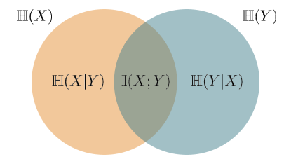
Figure 2: This venn diagram illustrates the relationships between the introduced information-theoretic quantities.

4.4 Differential Entropy

While we have defined information-theoretic quantities for discrete random variables, outside of mutual information we have not broached a notion of information regarding continuous random variables. For a continuous random variable $X:\Omega\mapsto\mathcal{X}$ with density $p_{X}$ (w.r.t the Lebesgue measure), we denote the differential entropy of $X$ by

$$\mathbf{h}(X)\ =\ \int_{x\in\mathcal{X}}p_{X}(x)\ln\frac{1}{p_{X}(x)}d\mu(x),$$

where $\mu(\cdot)$ denotes the Lebesgue measure. While differential entropy ostensibly resembles discrete entropy, the two are different in almost all regards. For instance, while the discrete entropy of a random variable is always non-negative, the differential entropy can often be negative. Look no further than $X=\text{Uniform}([0,1/2])$. In this case, $\mathbf{h}(X)=-\ln(2)$. Furthermore, while discrete entropy is invariant under one-to-one transformations, the differential entropy is not. For instance, $\mathbf{h}(2X)=\mathbf{h}(X)+\ln 2$. A measure of information should not be negative nor should it be dependent on units used. For these reasons, unlike discrete entropy, differential entropy is not a meaningful informational quantity by itself. The correct extension of discrete entropy to continuous random variables exists via rate-distortion theory, which we will present in the following section.

While differential entropy itself is not a meaningful measure of information, differences in (conditional) differential entropies are still equal to mutual information. Concretely, for continuous random variables $X,Y$ with finite (conditional) differential entropies,

$$\mathbb{I}(X;Y)\ =\ \mathbf{h}(X)-\mathbf{h}(X|Y)\ =\ \mathbf{h}(Y)-\mathbf{h}(Y|X).$$

4.5 Requisite Results from Information Theory

We now present an amalgamation of widely known and requisite results from information theory. Various proofs throughout this monograph will refer to the results of this section.

Lemma 6.

(log-sum inequality) For all $n\in\mathbb{Z}$, if $a_{1},\ldots,a_{n}\geq 0$, $b_{1},\ldots,b_{n}\geq 0$, and $a=\sum_{i=1}^{n}a_{i},b=\sum_{i=1}^{n}b_{i}$, then

$$\sum_{i=1}^{n}a_{i}\ln\frac{a_{i}}{b_{i}}\geq a\ln\frac{a}{b}.$$

Proof.

$$\sum_{i=1}^{n}a_{i}\ln\frac{a_{i}}{b_{i}} =\sum_{i=1}^{n}b_{i}\cdot\frac{a_{i}}{b_{i}}\ln\frac{a_{i}}{b_{i}}$$

$$=b\sum_{i=1}^{n}\frac{b_{i}}{b}\cdot\frac{a_{i}}{b_{i}}\ln\frac{a_{i}}{b_{i}}$$

$$\overset{(a)}{\geq}b\left(\sum_{i=1}^{n}\frac{b_{i}}{b}\cdot\frac{a_{i}}{b_{i}}\right)\ln\left(\sum_{i=1}^{n}\frac{b_{i}}{b}\cdot\frac{a_{i}}{b_{i}}\right)$$

$$=b\cdot\frac{a}{b}\ln\frac{a}{b}$$

$$=a\ln\frac{a}{b},$$

where (a) follows from Jensen’s inequality applied to the function $x\ln x$. ∎

Lemma 7.

(conditioning reduces entropy) For all discrete random variables $X:\Omega\mapsto\mathcal{X},Y:\Omega\mapsto\mathcal{Y}$,

$$\mathbb{H}(X)\geq\mathbb{H}(X|Y).$$

Proof.

$$\mathbb{H}(X) =\sum_{x\in\mathcal{X}}\mathbb{P}(X=x)\ln\frac{1}{\mathbb{P}(X=x)}$$

$$=\sum_{x\in\mathcal{X}}\sum_{y\in\mathcal{Y}}\mathbb{P}(X=x,Y=y)\ln\frac{1}{\mathbb{P}(X=x)}$$

$$\overset{(a)}{\geq}\sum_{x\in\mathcal{X}}\sum_{y\in\mathcal{Y}}\mathbb{P}(X=x,Y=y)\ln\frac{\mathbb{P}(Y=y)}{\mathbb{P}(X=x,Y=y)}$$

$$=\sum_{x\in\mathcal{X}}\sum_{y\in\mathcal{Y}}\mathbb{P}(X=x,Y=y)\ln\frac{1}{\mathbb{P}(X=x|Y=y)}$$

$$=\mathbb{H}(X|Y),$$

where $(a)$ follows from negating the log-sum inequality and setting $a_{i}=\mathbb{P}(X=x,Y=y),b_{i}=\mathbb{P}(Y=y)$ and $a=\mathbb{P}(X=x),b=1$. ∎

Lemma 8.

(conditioning reduces differential entropy) For all continuous random variables $X:\Omega\mapsto\mathcal{X},Y:\Omega\mapsto\mathcal{Y}$, if $\mathbf{h}(X),\mathbf{h}(X|Y)$ exist and are both finite, then

$$\mathbf{h}(X)\geq\mathbf{h}(X|Y).$$

Proof.

The proof follows from the same reasoning as in Lemma 7 by constructing a sequence of partitions of $\mathcal{X},\mathcal{Y}$ and taking the associated limits. ∎

Lemma 9.

(equivalence of mutual information and KL-divergence) For all random variables $X:\Omega\mapsto\mathcal{X},Y:\Omega\mapsto\mathcal{Y}$,

$$\mathbb{I}(X;Y)=\mathbb{E}\left[{\mathbf{d}}_{\rm KL}\left(\mathbb{P}(Y\in\cdot|X)\ \|\ \mathbb{P}(Y\in\cdot)\right)\right].$$

Proof.

We prove the result for discrete random variables $X,Y$. With appropriate technical assumptions, the result can also be extended to continual random variables which exhibit density functions.

$$\mathbb{I}(X;Y) =\sum_{x\in\mathcal{X}}\sum_{y\in\mathcal{Y}}\mathbb{P}(X=x,Y=y)\ln\frac{\mathbb{P}(X=x,Y=y)}{\mathbb{P}(X=x)\cdot\mathbb{P}(Y=y)}$$

$$=\sum_{x\in\mathcal{X}}\mathbb{P}(X=x)\sum_{y\in\mathcal{Y}}\mathbb{P}(Y=y|X=x)\ln\frac{\mathbb{P}(Y=y|X=x)}{\mathbb{P}(Y=y)}$$

$$=\mathbb{E}\left[{\mathbf{d}}_{\rm KL}\left(\mathbb{P}(Y\in\cdot|X)\ \|\ \mathbb{P}(Y\in\cdot)\right)\right].$$

∎

Lemma 10.

(non-negativity of KL-divergence) For all probability distributions $P(\cdot):\mathbb{F}\mapsto[0,1],Q(\cdot)\mathbb{F}\mapsto[0,1]$,

$${\mathbf{d}}_{\rm KL}\left(P(\cdot)\ \|\ Q(\cdot)\right)\geq 0.$$

Furthermore,

$${\mathbf{d}}_{\rm KL}(\left(P(\cdot)\ \|\ Q(\cdot)\right)=0\iff\text{ for all }\nu\in\mathbb{F},\left(P(\nu)>0\implies P(\nu)=Q(\nu)\right).$$

Proof.

$${\mathbf{d}}_{\rm KL}\left(P(\cdot)\ \|\ Q(\cdot)\right) =\sum_{\nu\in\mathbb{F}}P(\nu)\ln\frac{P(\nu)}{Q(\nu)}$$

$$=\sum_{\nu\in\mathbb{F}}-P(\nu)\ln\frac{Q(\nu)}{P(\nu)}$$

$$\overset{(a)}{\geq}-\ln\sum_{\nu\in\mathbb{F}}P(\nu)\cdot\frac{Q(\nu)}{P(\nu)}$$

$$=-\ln\sum_{\nu\in\mathbb{F}}Q(\nu)$$

$$=0.$$

where $(a)$ follows from Jensen’s inequality. To prove the second result, consider the case in which Jensen’s inequality holds with equality. This occurs iff $Q(\nu)/P(\nu)=\sum_{\nu\in\mathbb{F}}P(\nu)\cdot Q(\nu)/P(\nu)=1$. This occurs only when $Q(\nu)=P(\nu)$ for all $\nu\in\mathbb{F}$ for which $P(\nu)>0$. ∎

Lemma 11.

(maximum differential entropy) For all density functions $q:\Re^{d}\mapsto\Re_{+}$, for all $i,j\in[d]$, let $\Sigma_{i,j}=\int_{x\in\Re^{d}}x_{i}x_{j}q(x)dx$. If $X\sim\mathcal{N}(0,\Sigma)$, then

$$\mathbf{h}(X)\geq\int_{x\in\Re^{d}}q(x)\ln\frac{1}{q(x)}dx.$$

Proof.

Let $p$ denote the probability density function of $X$.

$$\mathbf{h}(X) =\int_{x\in\Re^{d}}-p(x)\left(\frac{1}{2}\ln(2\pi e|\Sigma|)-\frac{x^{\top}\Sigma^{-1}x}{2}\right)dx$$

$$=-\frac{1}{2}\ln\left(2\pi e|\Sigma|\right)+\int_{x\in\Re^{d}}p(x)\cdot\frac{x^{\top}\Sigma^{-1}x}{2}dx$$

$$\overset{(a)}{=}-\frac{1}{2}\ln\left(2\pi e|\Sigma|\right)+\int_{x\in\Re^{d}}q(x)\cdot\frac{x^{\top}\Sigma^{-1}x}{2}dx$$

$$=\int_{x\in\Re^{d}}q(x)\ln\frac{1}{p(x)}dx$$

$$=\int_{x\in\Re^{d}}q(x)\ln\frac{1}{q(x)}dx+{\mathbf{d}}_{\rm KL}\left(q(\cdot)\ \|\ p(\cdot)\right)$$

$$\overset{(b)}{\geq}\int_{x\in\Re^{d}}q(x)\ln\frac{1}{q(x)}dx$$

where $(a)$ follows from the equivalence of covariances assumption and $(b)$ follows from Lemma 10. ∎

Lemma 12.

(data processing inequality) Let $X,Y,Z$ be random variables for which $X\perp Z|Y$, then

$$\mathbb{I}(X;Z)\leq\mathbb{I}(Y;Z),\ \mathbb{I}(X;Z)\leq\mathbb{I}(X;Y).$$

$$\mathbb{I}(X;Z) \leq\mathbb{I}(X,Y;Z)$$

$$=\mathbb{I}(Y;Z)+\mathbb{I}(X;Z|Y)$$

$$\overset{(a)}{=}\mathbb{I}(Y;Z),$$

where $(a)$ follows from the independence assumption. Similarly,

$$\mathbb{I}(X;Z) \leq\mathbb{I}(X;Y,Z)$$

$$=\mathbb{I}(X;Y)+\mathbb{I}(X;Z|Y)$$

$$=\mathbb{I}(X;Y).$$

Summary

• The entropy of a discrete random variable $X:\Omega\mapsto\mathcal{X}$ is

  $$\mathbb{H}(X)=\sum_{x\in\mathcal{X}}\mathbb{P}(X=x)\ln\frac{1}{\mathbb{P}(X=x)}.$$

• The conditional entropy of a discrete random variable $X:\Omega\mapsto\mathcal{X}$ conditioned on another discrete random variable $Y:\Omega\mapsto\mathcal{Y}$ is

  $$\mathbb{H}(X|Y)=\sum_{x\in\mathcal{X},y\in\mathcal{Y}}\mathbb{P}(X=x,Y=y)\ln\frac{1}{\mathbb{P}(X=x|Y=y)}.$$

• The mutual information between two random variables $X:\Omega\mapsto\mathcal{X}$ and $Y:\Omega\mapsto\mathcal{Y}$ is

  $$\mathbb{I}(X;Y)\ =\ {\mathbf{d}}_{\rm KL}\left(\mathbb{P}((X,Y)\in\cdot)\|\mathbb{P}(X\in\cdot)\otimes\mathbb{P}(Y\in\cdot)\right),$$

  where $\mathbb{P}(X\in\cdot)\otimes\mathbb{P}(Y\in\cdot)$ denotes the outer product distribution. For discrete random variables,

  $$\mathbb{I}(X;Y)\ =\ \mathbb{H}(X)-\mathbb{H}(X|Y)\ =\ \mathbb{H}(Y)-\mathbb{H}(Y|X).$$

• (chain rule of mutual information) For all random variables $X:\Omega\mapsto\mathcal{X},Y:\Omega\mapsto\mathcal{Y},Z:\Omega\mapsto\mathcal{Z}$,

  $$\mathbb{I}(Y;Z|X)+\mathbb{I}(X;Z)=\mathbb{I}(X,Y;Z).$$

• The differential entropy of a continuous random variable $X:\Omega\mapsto\mathcal{X}$ with density $p_{X}$ (w.r.t the Lebesgue measure $\mu(\cdot)$) is

  $$\mathbf{h}(X)\ =\ \int_{x\in\mathcal{X}}p_{X}(x)\ln\frac{1}{p_{X}(x)}d\mu(x).$$

• Differential entropy can be negative and is unit-dependent.

• For continuous random variables $X:\Omega\mapsto\mathcal{X},Y:\Omega\mapsto\mathcal{Y}$,

  $$\mathbb{I}(X;Y)\ =\ \mathbf{h}(X)-\mathbf{h}(X|Y)\ =\ \mathbf{h}(Y)-\mathbf{h}(Y|X).$$

5 Connecting Learning and Information Theory

In this section, we will leverage the requisite information-theoretic results of section 4 to derive general upper and lower bounds for the estimation error of the Bayesian posterior $(\mathcal{L}_{T})$. The results of this section will facilitate the analysis of concrete problem instances in the following sections.

5.1 Error is Information

We now establish the elegant connection between $\mathcal{L}_{T}$ and mutual information.

Theorem 13.

(optimal error equals total information) For all $T\in\mathbb{Z}_{+}$,

$$\mathcal{L}_{T}=\frac{\mathbb{I}(H_{T};\theta)}{T}.$$

Proof.

$$\mathcal{L}_{T} =\frac{1}{T}\sum_{t=0}^{T-1}\mathbb{E}\left[-\ln\hat{P}_{t}(Y_{t+1})\right]-\frac{\mathbb{H}(Y_{1:T}|\theta,X_{0:T-1})}{T}$$

$$=\frac{1}{T}\sum_{t=0}^{T-1}\mathbb{E}\left[\ln\frac{\mathbb{P}(Y_{t+1}|\theta,H_{t})}{\hat{P}_{t}(Y_{t+1})}\right]$$

$$=\frac{1}{T}\sum_{t=0}^{T-1}\mathbb{E}\left[{\mathbf{d}}_{\rm KL}\left(\mathbb{P}(Y_{t+1}\in\cdot|\theta,H_{t})\ \|\ \mathbb{P}(Y_{t+1}\in\cdot|H_{t})\right)\right]$$

$$=\frac{1}{T}\sum_{t=0}^{T-1}\mathbb{I}(Y_{t+1};\theta|H_{t})$$

$$=\frac{1}{T}\sum_{t=0}^{T-1}\mathbb{I}(Y_{t+1};\theta|H_{t})+\mathbb{I}(X_{t};\theta|H_{t-1},Y_{t})$$

$$=\frac{\mathbb{I}(H_{T};\theta)}{T}.$$

∎

The estimation error incurred by an optimal algorithm over horizon $T$ is exactly equal to the total information acquired about $\theta$ from the observing the data $H_{T}$. Every nat of information about $\theta$ can only be acquired via incurring error on a prediction which relied on that information. Evidently, an optimal algorithm never makes the same mistake twice, hence resulting in the equality between total loss incurred and total information acquired. Results of a similar flavor appear in the global Fano’s method from the frequentist analysis of minimax lower bounds. However, the following connections to rate-distortion theory are novel.

A natural question which may arise when inspecting Theorem 13 is: “Does $\mathcal{L}_{T}$ decay to $0$ in $T$ and if so, at what rate?”. Ostensibly, the numerator $\mathbb{I}(\theta;H_{T})$ appears to be growing in $T$, so it is not immediately obvious that even an optimal learner will experience vanishing error. A simple instance to initially consider is $\theta$ which is a discrete random variable. In such an instance, we can always provide the upper bound:

$$\mathcal{L}_{T}\leq\frac{\mathbb{H}(\theta)}{T}.$$

Therefore, for any $\theta$ for which $\mathbb{H}(\theta)<\infty$, we have that $\mathcal{L}_{T}=O(1/T)$.

However, what about a more realistic scenario in which $\theta$ is a continuous random variable? A naive idea would be to simply supplant the discrete entropy $\mathbb{H}(\theta)$ with the differential entropy $\mathbf{h}(\theta)$. However, while differences in conditional differential entropy equal mutual information (just as with discrete entropy), differential entropy does not upper bound mutual information. This is because differential entropy can be negative (as discussed in section 4.4). The appropriate extension of discrete entropy to continuous random variables can be establish via rate-distortion theory.

5.2 Characterizing Error via Rate-Distortion Theory

We begin with the definition of the rate-distortion function.

Definition 14.

(rate-distortion function) Let $\epsilon\geq 0,\theta:\Omega\mapsto\Theta$ be a random variable, and $\rho$ a distortion function which maps $\theta$ and another random variable $\tilde{\theta}$ to $\Re_{+}$. The rate-distortion function evaluated for random variable $\theta$ at tolerance $\epsilon$ is defined as:

$$\inf_{\tilde{\theta}\in\tilde{\Theta}_{\epsilon}}\underbrace{\mathbb{I}(\theta;\tilde{\theta})}_{\rm rate},$$

where

$$\tilde{\Theta}_{\epsilon}=\left\{\tilde{\theta}:\underbrace{\mathbb{E}\left[\rho(\theta,\tilde{\theta})\right]}_{\rm distortion}\leq\epsilon\right\}.$$

Intuitively, one can think of $\tilde{\theta}$ as the result of passing $\theta$ through a noisy channel, resulting in a lossy compression. The objective $\mathbb{I}(\theta;\tilde{\theta})$, referred to as the rate, characterizes the number of nats that $\tilde{\theta}$ retains about $\theta$. meanwhile, the distortion function $\rho$ characterizes how lossy the compression is. The rate-distortion function returns the minimum number of nats necessary to achieve distortion at most $\epsilon$. In many ways this generalizes the concept of an $\epsilon$-cover in frequentist statistics. For the application of rate-distortion theory to the analysis of estimation error in machine learning, we consider the following distortion function:

$$\mathbb{E}\left[\rho_{t}(\theta,\tilde{\theta})\right] =\mathbb{E}\left[{\mathbf{d}}_{\rm KL}\left(\mathbb{P}(Y_{t+1}\in\cdot|\theta,H_{t})\ \|\ \mathbb{P}(Y_{t+1}\in\cdot|\tilde{\theta},H_{t})\right)\right]$$

$$=\mathbb{I}(Y_{t+1};\theta|\tilde{\theta},H_{t}),$$

where the second equality follows from the fact that $\tilde{\theta}\perp Y_{t+1}|(\theta,H_{t})$. This restriction ensure that $\tilde{\theta}$ does not contain exogenous information about $Y_{t+1}$ such as aleatoric noise which cannot be determined from $(\theta,H_{t})$. We use the notation $\mathbb{H}_{\epsilon,T}(\theta)$ to denote the following rate-distortion function:

$$\mathbb{H}_{\epsilon,T}(\theta)=\inf_{\tilde{\theta}\in\tilde{\Theta}_{\epsilon,T}}\ \mathbb{I}(\theta,\tilde{\theta}),$$

where

$$\tilde{\Theta}_{\epsilon,T}=\left\{\tilde{\theta}:\tilde{\theta}\perp H_{T}|\theta;\frac{\mathbb{I}(H_{T};\theta|\tilde{\theta})}{T}\leq\epsilon\right\}.$$

The following result upper and lower bounds the optimal estimation error in terms of the rate-distortion function:

Theorem 15.

(rate-distortion estimation error bounds) For all $T\in\mathbb{Z}_{+}$,

$$\sup_{\epsilon\geq 0}\ \min\left\{\frac{\mathbb{H}_{\epsilon,T}(\theta)}{T},\epsilon\right\}\ \leq\ \mathcal{L}_{T}\ \leq\ \inf_{\epsilon\geq 0}\ \frac{\mathbb{H}_{\epsilon,T}(\theta)}{T}+\epsilon.$$

Proof.

We begin with a proof of the upper bound.

$$\mathcal{L}_{T} =\frac{\mathbb{I}(H_{T};\theta)}{T}$$

$$=\frac{1}{T}\sum_{t=0}^{T-1}\mathbb{I}(Y_{t+1};\theta|H_{t})$$

$$=\frac{1}{T}\sum_{t=0}^{T-1}\mathbb{I}(Y_{t+1};\theta,\tilde{\theta}|H_{t})$$

$$=\frac{1}{T}\sum_{t=0}^{T-1}\mathbb{I}(Y_{t+1};\tilde{\theta}|H_{t})+\mathbb{I}(Y_{t+1};\theta|\tilde{\theta},H_{t})$$

$$=\frac{\mathbb{I}(H_{T};\tilde{\theta})}{T}+\frac{1}{T}\sum_{t=0}^{T-1}\mathbb{I}(Y_{t+1};\theta|\tilde{\theta},H_{t})$$

$$\overset{(a)}{\leq}\inf_{\epsilon\geq 0}\inf_{\tilde{\theta}\in\tilde{\Theta}_{\epsilon,T}}\ \frac{\mathbb{I}(\theta;\tilde{\theta})}{T}+\frac{1}{T}\sum_{t=0}^{T-1}\mathbb{I}(Y_{t+1};\theta|\tilde{\theta},H_{t})$$

$$=\inf_{\epsilon\geq 0}\inf_{\tilde{\theta}\in\tilde{\Theta}_{\epsilon,T}}\ \frac{\mathbb{I}(\theta;\tilde{\theta})}{T}+\frac{\mathbb{I}(H_{T};\theta|\tilde{\theta})}{T}$$

$$\leq\inf_{\epsilon\geq 0}\ \frac{\mathbb{H}_{\epsilon,T}(\theta)}{T}+\epsilon$$

where $(a)$ follows from the data processing inequality applied to the markov chain $\tilde{\theta}\perp H_{T}|\theta$.

We now proceed with the lower bound. Suppose that $\mathbb{I}(H_{T};\theta)<\mathbb{H}_{\epsilon,T}(\theta)$. Let $\tilde{\theta}=\tilde{H}_{T}\notin\tilde{\Theta}_{\epsilon,T}$ where $\tilde{H}_{T}$ is another history sampled in the same manner as $H_{T}$.

$$\mathbb{I}(H_{T};\theta) =\sum_{t=0}^{T-1}\mathbb{I}(Y_{t+1};\theta|H_{t})$$

$$\overset{(a)}{\geq}\sum_{t=0}^{T-1}\mathbb{I}(Y_{t+1};\theta|\tilde{H}_{t},H_{t})$$

$$=\sum_{t=0}^{T-1}\mathbb{I}(Y_{t+1};\theta|\tilde{\theta},H_{t})$$

$$\overset{(b)}{\geq}\epsilon T,$$

where $(a)$ follows from the fact that conditioning reduces entropy and that $Y_{t+1}\perp\tilde{H}_{t}|(\theta,H_{t})$ and $(b)$ follows from the fact that $\tilde{\theta}\notin\tilde{\Theta}_{\epsilon,T}$. Therefore, for all $\epsilon\geq 0$, $\mathbb{I}(H_{T};\theta)\geq\min\{H_{\epsilon,T},\epsilon T\}$. The result follows. ∎

Theorem 15 establishes the tight relation between estimation error and the rate-distortion function. The result is very general and facilitates the analysis of concrete problem instances in supervised learning. In the following section, we will study 3 concrete instances of increasing complexity to demonstrate how Theorem 15 facilitates analysis.

We also note the qualitative similarity between Theorem 15 and classical results from PAC learning which all characterize estimation error as a fraction involving a complexity function of the hypothesis space and the dataset size (VC-dimension, Rademacher complexity, log-covering number). In our framework, the rate-distortion function serves as the “complexity” function which characterizes the difficulty of learning $\theta$ for the purposes of prediction. In the following section, we will use this general result to derive concrete error bounds for a suite of problems involving data pairs which are iid when conditioned on $\theta$.

Summary

• (optimal estimation error equals total information) For horizon $T\in\mathbb{Z}_{+}$, the estimation error of the optimal algorithm is denoted as $\mathcal{L}_{T}$ and is

  $$\mathcal{L}_{T}=\frac{\mathbb{I}(\theta;H_{T})}{T}.$$

• For all $T\in\mathbb{Z}_{+}$,

  $$\mathcal{L}_{T}\leq\frac{\mathbb{H}(\theta)}{T}.$$

  Therefore, for a discrete random variable $\theta$ with finite entropy, $\mathcal{L}_{T}=O(1/T)$.

• The extension of this result to continuous random variables can be made via rate-distortion theory.

• (rate-distortion function) Let $\epsilon\geq 0,\theta:\Omega\mapsto\Theta$ be a random variable, and $\rho$ a distortion function which maps $\theta$ and another random variable $\tilde{\theta}$ to $\Re_{+}$. The rate-distortion function evaluated for random variable $\theta$ at tolerance $\epsilon$ is defined as:

  $$\inf_{\tilde{\theta}\in\tilde{\Theta}_{\epsilon}}\mathbb{I}(\theta;\tilde{\theta}),$$

  where

  $$\tilde{\Theta}_{\epsilon}=\left\{\tilde{\theta}:\mathbb{E}\left[\rho(\theta,\tilde{\theta})\right]\leq\epsilon\right\}.$$

• We use the notation $\mathbb{H}_{\epsilon,T}(\theta)$ to denote the following rate-distortion function:

  $$\mathbb{H}_{\epsilon,T}(\theta)=\inf_{\tilde{\theta}\in\tilde{\Theta}_{\epsilon,T}}\ \mathbb{I}(\theta,\tilde{\theta}),$$

  where

  $$\tilde{\Theta}_{\epsilon,T}=\left\{\tilde{\theta}:\tilde{\theta}\perp H_{T}|\theta;\frac{\mathbb{I}(H_{T};\theta|\tilde{\theta})}{T}\leq\epsilon\right\}.$$

• (rate-distortion estimation error bounds) For all $T\in\mathbb{Z}_{+}$,

  $$\sup_{\epsilon\geq 0}\ \min\left\{\frac{\mathbb{H}_{\epsilon,T}(\theta)}{T},\epsilon\right\}\ \leq\ \mathcal{L}_{T}\ \leq\ \inf_{\epsilon\geq 0}\ \frac{\mathbb{H}_{\epsilon,T}(\theta)}{T}+\epsilon.$$

6 Learning from iid Data

In this section, we restrict our attention to the analysis of learning under independently and identically distributed (iid) data. Concretely, we assume that the random process representing the inputs: $(X_{0},X_{1},\ldots)$ is iid. Each input $X_{t}$ is associated with a label $Y_{t+1}$ and we assume infinite exchangeability of the sequence $((X_{0},Y_{1}),(X_{1},Y_{1}),\ldots)$. By de Finetti’s theorem, there exists a latent random variable, which we denote by $\theta$, for which conditioned on $\theta$, the above sequence is iid. We further make the standard assumption that the sequence of inputs $(X_{0},X_{1},\ldots)$ is independent of $\theta$. As a result, $\theta$ is a random variable which represents for all $t$ the conditional probability measure $\theta(\cdot|X_{t})$ of $Y_{t+1}$. The process of learning involves the reduction of uncertainty about $\theta$ in ways which are relevant for future predictions.

In the following section, we provide several results which follow as a consequence of the above iid assumption. We dedicate the remaining sections to studying 4 concrete problem instances of increasing complexity: $1)$ linear regression, $2)$ logistic regression, $3)$ deep neural networks, $4)$ non-parametric learning. We hope that this suite of examples provide the reader with enough intuition and tools to analyze their own problems of interest.

6.1 Theoretical Results Tailored for iid Data

We begin with several intuitive theoretical results which follow as a result of the iid assumptions on the data. The first result establishes monotonicity of estimation error:

Lemma 16.

(monotonicity of per-timestep estimation error) If $((X_{t},Y_{t+1}:t\in\mathbb{Z}_{+})$ is an iid stochastic process when conditioned on $\theta$, then for all $t\in\mathbb{Z}_{+}$,

$$\mathbb{I}(Y_{t+2};\theta|H_{t+1})\ \leq\ \mathbb{I}(Y_{t+1};\theta|H_{t}).$$

Proof.

We have

$$\mathbb{I}(\theta;Y_{t+2}|H_{t+1}) =\mathbf{h}(Y_{t+2}|H_{t+1})-\mathbf{h}(Y_{t+2}|\theta,H_{t+1})$$

$$\overset{(a)}{=}\mathbf{h}(Y_{t+2}|H_{t+1})-\mathbf{h}(Y_{t+2}|\theta,H_{t-1},Y_{t},X_{t+1})$$

$$\overset{(b)}{\leq}\mathbf{h}(Y_{t+2}|H_{t-1},Y_{t},X_{t+1})-\mathbf{h}(Y_{t+2}|\theta,H_{t-1},Y_{t},X_{t+1})$$

$$=\mathbb{I}(Y_{t+2};\theta|H_{t-1},Y_{t},X_{t+1})$$

$$\overset{(c)}{=}\mathbb{I}(Y_{t+1};\theta|H_{t-1},Y_{t},X_{t})$$

$$=\mathbb{I}(Y_{t+1};\theta|H_{t}),$$

where $(a)$ follows since $Y_{t+2}\perp(X_{t},Y_{t+1})|(\theta,X_{t+1})$, $(b)$ follows from the fact that conditioning reduces differential entropy, and $(c)$ follows from the fact that $(X_{t},Y_{t+1})$ and $(X_{t+1},Y_{t+2})$ are identically distributed conditioned on $(H_{t-1},Y_{t})$. ∎

The above result establishes that when the data generating process is iid conditioned on $\theta$, the optimal per-timestep estimation error is monotonically non-increasing. This is intuitive, if the data is iid, the future sequence is exchangeable and hence, conditioning on additional information ($H_{t+1}$ as opposed to $H_{t}$) should only improve our ability to make predictions. A corollary of this result is that for iid data, we can upper bound distortion via an expression which is much simpler to analyze.

Corollary 17.

(distortion upper bound) If $((X_{t},Y_{t+1}:t\in\mathbb{Z}_{+})$ is an iid stochastic process when conditioned on $\theta$ and for all $t\in\mathbb{Z}_{+}$, $Y_{t+1}\perp\tilde{\theta}|(\theta,X_{t})$, then for all $T\in\mathbb{Z}_{++}$,

$$\frac{\mathbb{I}(H_{T};\theta|\tilde{\theta})}{T}\ \leq\ \mathbb{I}(Y_{1};\theta|\tilde{\theta},X_{0}).$$

Proof.

$$\frac{\mathbb{I}(H_{T};\theta|\tilde{\theta})}{T} =\frac{1}{T}\sum_{t=0}^{T-1}\mathbb{I}(X_{t},Y_{t+1};\theta|\tilde{\theta},H_{t-1},Y_{t})$$

$$\overset{(a)}{=}\frac{1}{T}\sum_{t=0}^{T-1}\mathbb{I}(Y_{t+1};\theta|\tilde{\theta},H_{t})$$

$$\overset{(b)}{\leq}\mathbb{I}(Y_{1};\theta|\tilde{\theta},X_{0})$$

where $(a)$ follows from the assumption that $X_{t}\perp\theta$ and $(b)$ follows from the same proof technique as in Lemma 16. ∎

In general, the expression $\mathbb{I}(H_{T};\theta|\tilde{\theta})$ is much more cumbersome to deal with in comparison to $\mathbb{I}(Y_{1};\theta|\tilde{\theta},X_{0})$. Corollary 17 established a suitable relationship between the two quantities. However, to facilitate the analysis of rate-distortion lower bounds, it is fruitful to consider analysis via a modified rate-distortion function tailored for iid data generating processes. For all $\epsilon\geq 0$, we let

$$\mathbb{H}_{\epsilon}(\theta)=\inf_{\tilde{\theta}\in\tilde{\Theta}_{\epsilon}}\mathbb{I}(\theta;\tilde{\theta}),$$

where

$$\tilde{\Theta}_{\epsilon}=\{\tilde{\theta}:\tilde{\theta}\perp H_{\infty}|\theta,\ \mathbb{I}(Y_{1};\theta|\tilde{\theta},X_{0})\leq\epsilon\}.$$

Note that in contrast to the general rate-distortion formulation of section 5, this modified rate-distortion does not depend on the time horizon $T$. We now provide an estimation error lower bound in terms of $\mathbb{H}_{\epsilon}(\theta)$ which applies for learning from iid data.

Lemma 18.

(estimation error lower bound for iid data) If $((X_{t},Y_{t+1}:t\in\mathbb{Z}_{+})$ is an iid stochastic process when conditioned on $\theta$, then for all $T\in\mathbb{Z}_{++},$

$$\sup_{\epsilon\geq 0}\ \min\left\{\frac{\mathbb{H}_{\epsilon}(\theta)}{T},\epsilon\right\}\ \leq\ \mathcal{L}_{T}.$$

Proof.

Fix $T\in\mathbb{Z}_{+}$. Let $\tilde{\theta}=(\tilde{H}_{T-2},\tilde{Y}_{T-1})$ be independent from but distributed identically with $(H_{T-2},Y_{T-1})$ when conditioned on $\theta$.

Fix $\epsilon\geq 0$. If $\mathcal{L}_{T}<\mathbb{H}_{\epsilon}(\theta)/T$ then

$$\mathcal{L}_{T}<\mathbb{H}_{\epsilon}(\theta)/T\ \implies\ \mathbb{I}(H_{T};\theta)<\mathbb{H}_{\epsilon}(\theta)\ \implies\ \mathbb{I}(\tilde{\theta};\theta)<\mathbb{H}_{\epsilon}(\theta).$$

Since the rate of $\tilde{\theta}$ is lower than the rate-distortion function $\mathbb{H}_{\epsilon}(\theta)$, $\tilde{\theta}\notin\tilde{\Theta}_{\epsilon}$. As a result,

$$\mathcal{L}_{T} \overset{(a)}{=}\frac{\mathbb{I}(H_{T};\theta)}{T}$$

$$\overset{(b)}{=}\frac{1}{T}\sum_{t=0}^{T-1}\mathbb{I}(Y_{t+1};\theta|H_{t})$$

$$\overset{(c)}{\geq}\mathbb{I}(Y_{T};\theta|H_{T-1})$$

$$=\mathbb{I}(Y_{T};\theta|\tilde{\theta},X_{T-1})$$

$$\overset{(d)}{>}\epsilon,$$

where (a) follows from Lemma 13, (b) follows from the chain rule of mutual information, (c) follows from Lemma 16, and (d) follows from the fact that $\tilde{\theta}\notin\tilde{\Theta}_{\epsilon}$. Therefore,

$$\mathcal{L}_{T}\geq\min\{\mathbb{H}_{\epsilon}(\theta)/T,\ \epsilon\}.$$

Since this holds for any $\epsilon\geq 0$, the result follows. ∎

In the following $4$ sections we will apply our general results to concrete problem instances. We begin with linear regression.

6.2 Linear Regression

Figure 3: We depict our linear regression data generating process above. It consists of an input vector $X$ of dimension $d$, an unknown weight vector $\theta$ of dimension $d$, and a final output $Y$ which is the sum of $\theta^{\top}X$ and independent Gaussian noise $Z$.

6.2.1 Data Generating Process

In linear regression, the variable that we are interested in estimating is a random vector $\theta\in\Re^{d}$. As our analytical tools are developed in a Bayesian framework, we assume a known prior distribution $\mathbb{P}(\theta\in\cdot)$ to model our uncertainty over the value of $\theta$. For simplicity and concreteness, in this example, we assume that $\mathbb{P}(\theta\in\cdot)=\mathcal{N}(0,I_{d}/d)$. For all $t\in\mathbb{Z}_{+}$, inputs and outputs are generated according to a random vector $X_{t}\overset{iid}{\sim}\mathcal{N}(0,I_{d})$ and

$$Y_{t+1}=\theta^{\top}X_{t}+W_{t+1},$$

where $W_{t}\overset{iid}{\sim}\mathcal{N}(0,\sigma^{2})$ for known variance $\sigma^{2}$. We note that the results and techniques developed in this section certainly extend to input and prior distributions which are not Gaussian with slight modifications. We study the Gaussian case as it minimizes ancillary clutter without compromising generality. In the following section, we will establish a series of smaller results which will allow us to streamline our error analysis using the tools established in section 5.

6.2.2 Theoretical Building Blocks

In this section we will establish $3$ relatively simple results which will enable us to directly apply Theorem 15 and arrive at estimation error bounds for linear regression. As such, the results will all involve characterizing the rate-distortion function for this data generating process. We begin our analysis with a result which establishes the threshold $\epsilon$ at which the rate-distortion function is trivially $0$.

Lemma 19.

(linear regression 0 rate-distortion threshold) For all $d\in\mathbb{Z}_{++},\sigma^{2}\in\Re_{++}$, if for all $t\in\mathbb{Z}_{+}$, $(X_{t},Y_{t+1})$ are generated according to the linear regression process and $\epsilon\geq\frac{1}{2}\ln(1+1/\sigma^{2})$, then for all $T\in\mathbb{Z}_{++}$,

$$\mathbb{H}_{\epsilon,T}(\theta)=0.$$

Proof.

Let $\tilde{\theta}=\emptyset$. Then,

$$\frac{\mathbb{I}(H_{T};\theta|\tilde{\theta})}{T} \overset{(a)}{\leq}\mathbb{I}(Y_{1};\theta|\tilde{\theta},X_{0})$$

$$=\mathbf{h}(Y_{1}|\tilde{\theta},X_{0})-\mathbf{h}(Y_{1}|\theta,\tilde{\theta},X_{0})$$

$$=\mathbf{h}(Y_{1}|X_{0})-\mathbf{h}(W)$$

$$\overset{(b)}{\leq}\mathbb{E}\left[\frac{1}{2}\ln\left(2\pi e\left(\sigma^{2}+\text{Var}[\theta^{\top}X|X]\right)\right)\right]-\frac{1}{2}\ln\left(2\pi e\sigma^{2}\right)$$

$$\overset{(c)}{=}\mathbb{E}\left[\frac{1}{2}\ln\left(2\pi e\left(\sigma^{2}+\frac{\|X\|^{2}_{2}}{d}\right)\right)\right]-\frac{1}{2}\ln\left(2\pi e\sigma^{2}\right)$$

$$\overset{(d)}{\leq}\frac{1}{2}\ln\left(2\pi e\left(\sigma^{2}+\frac{\mathbb{E}\left[\|X\|^{2}_{2}\right]}{d}\right)\right)-\frac{1}{2}\ln\left(2\pi e\sigma^{2}\right)$$

$$=\frac{1}{2}\ln\left(1+\frac{1}{\sigma^{2}}\right)$$

$$\leq\epsilon,$$

where $(a)$ follows from Corollary 17, $(b)$ follows from Lemma 11, $(c)$ follows from the fact that $\theta$ has covariance matrix $I_{d}/d$, and $(d)$ follows from Jensen’s inequality. The above establishes that $\tilde{\theta}\in\tilde{\Theta}_{\epsilon,T}$ for all $T$. The result follows from the fact that $\mathbb{I}(\theta;\tilde{\theta})=0$. ∎

Intuitively, there should be a threshold of $\epsilon$ for which values greater than $\epsilon$ result in a rate-distortion value of $0$. Evidently, a $0$-bit quantization that solely relies on the prior distribution will result in a suitable distortion value when the threshold $\epsilon$ is large enough. This result characterizes the edge-case condition for the rate-distortion function. The following result will provide an upper bound on the rate-distortion function for the more interesting scenario in which the threshold $\epsilon<1/2\ln(1+1/\sigma^{2})$.

Lemma 20.

(linear regression rate-distortion upper bound) For all $d\in\mathbb{Z}_{++}$, $\sigma^{2}\in\Re_{++}$, and $\epsilon\in\Re_{++}$, if for all $t\in\mathbb{Z}_{+}$, $(X_{t},Y_{t+1})$ are generated according to the linear regression process, then for all $T$,

$$\mathbb{H}_{\epsilon,T}(\theta)\leq\left(\frac{d}{2}\ln\left(\frac{1}{\sigma^{2}(e^{2\epsilon}-1)}\right)\right)_{+}.$$

Proof.

Fix $\sigma^{2}\in\Re_{++}$. Let $\tilde{\theta}=\theta+V$, where $V\sim\mathcal{N}(0,(\delta^{2}/d)I_{d})$ for $\delta^{2}=\frac{\sigma^{2}(e^{2\epsilon}-1)}{1-\sigma^{2}(e^{2\epsilon}-1)}$ and $V\perp\theta$. Note that $\delta^{2}\geq 0$ for all $0<\epsilon<\frac{1}{2}\ln\left(1+\frac{1}{\sigma^{2}}\right)$. We begin by showing that $\tilde{\theta}\in\tilde{\Theta}_{\epsilon,T}$ for all $T$.

$$\frac{\mathbb{I}(H_{T};\theta|\tilde{\theta})}{T} \leq\mathbb{I}(Y_{1};\theta|\tilde{\theta},X_{0})$$

$$=\mathbf{h}(Y_{1}|\tilde{\theta},X_{0})-\mathbf{h}(Y_{1}|\theta,\tilde{\theta},X_{0})$$

$$=\mathbf{h}(W_{1}+\theta^{\top}X|\tilde{\theta},X_{0})-\mathbf{h}(W_{1})$$

$$=\mathbf{h}\left(W_{1}+\theta^{\top}X_{0}-\frac{\tilde{\theta}^{\top}X_{0}}{1+\delta^{2}}\bigg{|}\tilde{\theta},X_{0}\right)-\mathbf{h}(W_{1})$$

$$=\mathbf{h}\left(W_{1}+\left(\frac{\delta^{2}}{1+\delta^{2}}\theta+\frac{1}{1+\delta^{2}}V\right)^{\top}X_{0}\Big{|}\tilde{\theta},X_{0}\right)-\mathbf{h}(W_{1})$$

$$\leq\mathbf{h}\left(W_{1}+\left(\frac{\delta^{2}}{1+\delta^{2}}\theta+\frac{1}{1+\delta^{2}}V\right)^{\top}X_{0}\Big{|}X_{0}\right)-\mathbf{h}(W_{1})$$

$$\overset{(a)}{\leq}\mathbb{E}\left[\frac{1}{2}\ln\left(2\pi e\left(\sigma^{2}+\left(\frac{\delta^{4}}{d(1+\delta^{2})^{2}}+\frac{\delta^{2}}{d(1+\delta^{2})^{2}}\right)\|X_{0}\|^{2}_{2}\right)\right)\right]-\frac{1}{2}\ln\left(2\pi e\sigma^{2}\right)$$

$$=\mathbb{E}\left[\frac{1}{2}\ln\left(1+\frac{\delta^{2}\|X_{0}\|^{2}_{2}}{d(1+\delta^{2})\sigma^{2}}\right)\right]$$

$$\overset{(b)}{\leq}\frac{1}{2}\ln\left(1+\frac{\delta^{2}}{(1+\delta^{2})\sigma^{2}}\right)$$

$$=\frac{1}{2}\ln\left(e^{2\epsilon}\right)$$

$$=\epsilon,$$

where $(a)$ follows from Lemma 11 and $(b)$ follows from Jensen’s inequality. Next, we upper bound the rate of $\tilde{\theta}$:

$$\mathbb{I}(\theta;\tilde{\theta}) =\mathbf{h}(\tilde{\theta})-\mathbf{h}(\tilde{\theta}|\theta)$$

$$=\mathbf{h}(\tilde{\theta})-\mathbf{h}(V)$$

$$\overset{(a)}{\leq}\frac{d}{2}\ln\left(2\pi e\left(\frac{\delta^{2}+1}{d}\right)\right)-\frac{d}{2}\ln\left(2\pi e\left(\frac{\delta^{2}}{d}\right)\right)$$

$$=\frac{d}{2}\ln\left(1+\frac{1}{\delta^{2}}\right)$$

$$=\frac{d}{2}\ln\left(\frac{1}{\sigma^{2}\left(e^{2\epsilon}-1\right)}\right),$$

where $(a)$ follows from Lemma 11. The result follows from Lemma 19 and the fact that $\tilde{\theta}\in\tilde{\Theta}_{\epsilon,T}$ for all $T\in\mathbb{Z}_{++}$ and $\epsilon<1/2\ln(1+1/\sigma^{2})$. ∎

Note that above, we never explicitly relied on the assumption that $\mathbb{P}(\theta\in\cdot)=\mathcal{N}(0,I_{d}/d)$. We simply needed the fact that the elements of $\theta$ are independent with variances which sum to $1$ (for inequality $(a)$ above). To establish a lower bound on the rate-distortion function in the linear regression setting, we rely more on the Gaussian prior assumption. Concrete details of the most general assumptions required to arrive at such lower bounds can be found in Appendix A.

Lemma 21.

(linear regression rate-distortion lower bound) For all $d\in\mathbb{Z}_{++}$ s.t. $d>2$, $\sigma^{2}\in\Re_{++}$, and $\epsilon\in\Re_{++}$, if for all $t\in\mathbb{Z}_{+}$, $(X_{t},Y_{t+1})$ are generated according to the linear regression process, then

$$\mathbb{H}_{\epsilon}(\theta)\ \geq\ \left(\frac{d}{2}\ln\left(\frac{1}{(8+\frac{d}{d-2}\sigma^{2})\epsilon}\right)\right)_{+}.$$

Proof.

Fix $\sigma^{2}\in\Re_{++}$, $\epsilon\in\mathbb{Z}_{+}$ $T\in\mathbb{Z}_{++}$, and $\tilde{\theta}\in\tilde{\Theta}_{\epsilon,T}$. Then,

$$\epsilon \overset{(a)}{\geq}\mathbb{I}(Y;\theta|\tilde{\theta},X)$$

$$\overset{(b)}{\geq}\mathbb{E}\left[\frac{\|X\|^{2}_{2}}{2(4\|X\|_{2}^{2}+d\sigma^{2})}\right]\mathbb{E}\left[\|\theta-\mathbb{E}[\theta|\tilde{\theta}]\|^{2}_{2}\right]$$

$$=\mathbb{E}\left[\frac{1}{\frac{2(4\|X\|_{2}^{2}+d\sigma^{2})}{\|X\|_{2}^{2}}}\right]\mathbb{E}\left[\|\theta-\mathbb{E}[\theta|\tilde{\theta}]\|^{2}_{2}\right]$$

$$=\mathbb{E}\left[\frac{1}{8+\frac{d\sigma^{2}}{\|X\|^{2}_{2}}}\right]\mathbb{E}\left[\|\theta-\mathbb{E}[\theta|\tilde{\theta}]\|^{2}_{2}\right]$$

$$\overset{(c)}{\geq}\frac{1}{\mathbb{E}\left[8+\frac{d\sigma^{2}}{\|X\|^{2}_{2}}\right]}\mathbb{E}\left[\|\theta-\mathbb{E}[\theta|\tilde{\theta}]\|^{2}_{2}\right]$$

$$\overset{(d)}{=}\frac{1}{8+\frac{d\sigma^{2}}{d-2}}\mathbb{E}\left[\|\theta-\mathbb{E}[\theta|\tilde{\theta}]\|^{2}_{2}\right]$$

$$\geq\frac{1}{8+\frac{d}{d-2}\sigma^{2}}\mathbb{E}\left[\|\theta-\mathbb{E}[\theta|\tilde{\theta}]\|^{2}_{2}\right]$$

where $(a)$ follows from the fact that $\tilde{\theta}\in\tilde{\Theta}_{\epsilon}$, $(b)$ follows from Lemma 63, $(c)$ follows from Jensen’s inequality, and $(d)$ follows from the fact that $\mathbb{E}[1/\chi^{2}(d)]=1/(d-2)$.

Since the above condition is an implication that holds for arbitrary $\tilde{\theta}\in\tilde{\Theta}_{\epsilon}$, minimizing the rate $\mathbb{I}(\theta;\tilde{\theta})$ over the set of proxies that satisfy $\mathbb{E}[\|\theta-\mathbb{E}[\theta|\tilde{\theta}]\|^{2}_{2}]\leq(8+\frac{d}{d-2}\sigma^{2})\epsilon$ will provide a lower bound. However, this is simply the rate-distortion problem for a multivariate source under squared error distortion. For this problem there exists a well known lower bound (Theorem 10.3.3 of [Cover and Thomas, 2006]). The lower bound follows as a result.
∎

6.2.3 Main Result

The rate-distortion bounds which we established in the previous section allow us to directly apply Theorem 15 to arrive at a bound for estimation error.

Theorem 22.

(linear regression estimation error bounds) For all $d\in\mathbb{Z}_{++}$, $\sigma^{2}\geq 0$, if for all $t$, $(X_{t},Y_{t+1})$ are generated according to the linear regression processes, then for all $T$,

$$\frac{d}{2T}W\left(\frac{2T}{d(8+\frac{d}{d-2}\sigma^{2})}\right)\ \leq\ \mathcal{L}_{T}\ \leq\ \left(\frac{d}{2T}\ln\left(\frac{T}{\sigma^{2}d}\right)\right)_{+}+\frac{1}{2T}\ln\left(1+\frac{d}{T}\right),$$

where $W$ is the Lambert W function.

Proof.

$$\mathcal{L}_{T} \overset{(a)}{\leq}\inf_{\epsilon\geq 0}\ \frac{\mathbb{H}_{\epsilon,T}(\theta)}{T}+\epsilon$$

$$\overset{(b)}{\leq}\inf_{\epsilon\geq 0}\ \frac{\left(d\ln\left(\frac{1}{\sigma^{2}(e^{2\epsilon}-1)}\right)\right)_{+}}{2T}+\epsilon$$

$$\overset{(c)}{\leq}\frac{\left(d\ln\left(\frac{1}{\sigma^{2}\left(\left(1+\frac{d}{T}\right)^{T}-1\right)}\right)\right)_{+}}{2T}+\frac{1}{2T}\ln\left(1+\frac{d}{T}\right)$$

$$\leq\left(\frac{d}{2T}\ln\left(\frac{T}{\sigma^{2}d}\right)\right)_{+}+\frac{1}{2T}\ln\left(1+\frac{d}{T}\right),$$

where $(a)$ follows from Theorem 15, $(b)$ follows from Lemma 20, and $(c)$ follows from setting $\epsilon=\frac{1}{2T}\ln\left(1+\frac{d}{T}\right)$.

$$\mathcal{L}_{T} \geq\sup_{\epsilon\geq 0}\ \min\left\{\frac{\mathbb{H}_{\epsilon}(\theta)}{T},\epsilon\right\}$$

$$\geq\sup_{\epsilon\geq 0}\ \min\left\{\left(\frac{d}{2T}\ln\left(\frac{1}{(8+\frac{d}{d-2}\sigma^{2})\epsilon}\right)\right)_{+},\ \epsilon\right\}$$

$$=\epsilon\text{ s.t. }\left(\frac{d}{2T}\ln\left(\frac{1}{(8+\frac{d}{d-2}\sigma^{2})\epsilon}\right)\right)_{+}=\epsilon$$

$$\overset{(a)}{=}\frac{e^{-W\left(\frac{8+\frac{d}{d-2}\sigma^{2}}{2}\right)}}{\frac{2T}{d(8+\frac{d}{d-2}\sigma^{2})}}$$

$$\overset{(b)}{\geq}\frac{e^{-\ln\left(8+\frac{d}{d-2}\sigma^{2}\right)}}{\frac{2T}{d(8+\frac{d}{d-2}\sigma^{2})}}$$

$$=\frac{d}{2T},$$

where in $(a)$, $W$ denotes the Lambert $W$ function and $(b)$ follows from the fact that for all $x\geq e$, $W(x)\leq\ln(2x)$. ∎

Notably, this bound is consistent with classical results in statistics which dictate that the estimation error grows linearly in the problem dimension $d$ and decays linearly in the number of samples observed $T$. In the following section, we will observe that qualitatively similar results also hold for logistic regression.

6.3 Logistic Regression

Figure 4: We depict our logistic regression data generating process above. It consists of an input vector $X$ of dimension $d$, an unknown weight vector $\theta$ of dimension $d$, and a final binary output $Y\in\{0,1\}$. $Y$ is sampled according to probabilities generated by the sigmoid function applied to $\theta^{\top}X$.

6.3.1 Data Generating Process

We next study logistic regression to demonstrate the application of our tools to classification. Just as in linear regression, in logistic regression, the variable that we are interested in estimating is a random vector $\theta\in\Re^{d}$. Again for simplicity and concreteness, we assume that $\mathbb{P}(\theta\in\cdot)=\mathcal{N}(0,I_{d}/d)$. For all $t\in\mathbb{Z}_{+}$, inputs and outputs are generated according to a random vector $X_{t}\overset{iid}{\sim}\mathcal{N}(0,I_{d})$ and

$$Y_{t+1}=\begin{cases}1&\text{ w.p. }\frac{1}{1+e^{-\theta^{\top}X_{t}}}\\ 0&\text{ otherwise}\end{cases}.$$

6.3.2 Theoretical Building Blocks

We begin with the following result which upper bounds the binary KL-divergence of a sigmoidal output via the squared difference between the logits.

Lemma 23.

(squared error upper bounds binary KL-divergence) For all $x,y\in\Re$,

$$\frac{1}{1+e^{-x}}\ln\frac{1+e^{-y}}{1+e^{-x}}+\frac{1}{1+e^{x}}\ln\frac{1+e^{y}}{1+e^{x}}\leq\frac{(x-y)^{2}}{8}$$

Proof.

∎

This upper bound facilitates the following upper bound on the rate-distortion function.

Lemma 24.

(logistic regression rate-distortion upper bound) For all $d\in\mathbb{Z}_{++}$ and $\epsilon\in\Re_{++}$, if for all $t\in\mathbb{Z}_{+},(X_{t},Y_{t+1})$ are generated according to the logistic regression process, then for all $T$,

$$\mathbb{H}_{\epsilon,T}\ \leq\ \frac{d}{2}\ln\left(1+\frac{1}{8\epsilon}\right).$$

Proof.

Let $\tilde{\theta}=\theta+Z$ where $Z\perp\theta$ and $Z\sim\mathcal{N}(0,8\epsilon/d)$. Then,

$$\frac{\mathbb{I}(H_{T};\theta|\tilde{\theta})}{T} \leq\mathbb{I}(Y_{1};\theta|\tilde{\theta},X_{0})$$

$$=\mathbb{E}\left[{\mathbf{d}}_{\rm KL}\left(\mathbb{P}(Y_{1}\in\cdot|\theta,X_{0})\ \|\ \mathbb{P}(Y_{1}\in\cdot|\tilde{\theta},X_{0})\right)\right]$$

$$\overset{(a)}{\leq}\mathbb{E}\left[{\mathbf{d}}_{\rm KL}\left(\mathbb{P}(Y_{1}\in\cdot|\theta,X_{0})\ \|\ \mathbb{P}(Y_{1}\in\cdot|\theta\leftarrow\tilde{\theta},X_{0})\right)\right]$$

$$=\mathbb{E}\left[\frac{\ln\left(\frac{1+e^{-\tilde{\theta}^{\top}X_{0}}}{1+e^{-\theta^{\top}X_{0}}}\right)}{1+e^{-\theta^{\top}X_{0}}}+\frac{\ln\left(\frac{1+e^{\tilde{\theta}^{\top}X_{0}}}{1+e^{\theta^{\top}X_{0}}}\right)}{1+e^{\theta^{\top}X_{0}}}\right]$$

$$\overset{(b)}{\leq}\frac{\mathbb{E}\left[\left(\theta^{\top}X_{0}-\tilde{\theta}^{\top}X_{0}\right)^{2}\right]}{8}$$

$$=\frac{\mathbb{E}\left[\|\theta-\tilde{\theta}\|^{2}_{2}\right]}{8}$$

$$=\epsilon,$$

where $(a)$ follows from Lemma 57 and $(b)$ follows from Lemma 23.

We now upper bound the rate.

$$\mathbb{I}(\theta;\tilde{\theta}) =\mathbf{h}(\tilde{\theta})-\mathbf{h}(\tilde{\theta}|\theta)$$

$$\overset{(a)}{\leq}\frac{d}{2}\ln\left(2\pi e\left(\frac{1}{d}+\frac{8\epsilon}{d}\right)\right)-\frac{d}{2}\ln\left(2\pi e\frac{8\epsilon}{d}\right)$$

$$=\frac{d}{2}\ln\left(1+\frac{1}{8\epsilon}\right),$$

where $(a)$ follows from Lemma 11. The result follows. ∎

6.3.3 Main Result

With the rate-distortion upper bound in place, we establish the following upper bound on estimation error.

Theorem 25.

(logistic regression estimation error upper bound) For all $d\in\mathbb{Z}_{++}$, if for all $t$, $(X_{t},Y_{t+1})$ is generated according to the logistic regression process, then for all $T,$

$$\mathcal{L}_{T}\ \leq\ \frac{d}{2T}\left(1+\ln\left(1+\frac{T}{4d}\right)\right).$$

Proof.

$$\mathcal{L}_{T} \overset{(a)}{\leq}\inf_{\epsilon\geq 0}\ \frac{\mathbb{H}_{\epsilon,T}(\theta)}{T}+\epsilon$$

$$\overset{(b)}{\leq}\inf_{\epsilon\geq 0}\ \frac{\frac{d}{2}\ln\left(1+\frac{d}{8\epsilon}\right)}{T}+\epsilon$$

$$\overset{(c)}{\leq}\frac{d}{2T}\ln\left(1+\frac{T}{4d}\right)+\frac{d}{2T},$$

where $(a)$ follows from Theorem 15, $(b)$ follows from Lemma 24, and $(c)$ follows from setting $\epsilon=\frac{d}{2T}$. ∎

We observe that just as in linear regression, we observe an error bound which is $\tilde{\mathcal{O}}(d/T)$. In the following section, we consider a much more complex deep neural network data generating process.

6.4 Deep Neural Networks

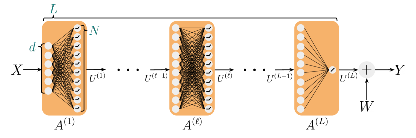
Figure 5: We depict our deep neural network data generating process above. It consists of input dimension $d$, width $N$, depth $L$, with output dimension $1$, and ReLU activation units. We denote the weights at layer $\ell$ by $A^{(\ell)}$ and the output of layer $\ell$ by $U^{(\ell)}$. We assume that the final output $Y$ is the sum of the final network output $U^{(L)}$ and independent Gaussian noise $Z$.

6.4.1 Data Generating Process

For a deep neural network, we are interested in estimating a collection of random matrices $(A^{(1)},\ldots,A^{(L)})$ which represent the weights of the network. We assume a known prior distribution $\mathbb{P}(A^{(1:L)}\in\cdot)$ to model our uncertainty over the network weights. For simplicity, we assume that the width of every hidden layer is identically set to a positive integer $N$ and that the network has input dimension $d$ and output dimension $1$. We further assume the following prior distribution on the weights of the network.

$$\mathbb{P}(A^{(\ell)})=\begin{cases}\mathcal{N}(0,\frac{I_{N\times d}}{d})&\text{ if }\ell=1\\ \mathcal{N}(0,\frac{I_{N\times N}}{N})&\text{ if }2\leq\ell\leq L-1\\ \mathcal{N}(0,\frac{I_{N}}{N})&\text{ if }\ell=L\end{cases}.$$

We further make the assumption that the weights across layers are independent. These Gaussian assumptions are again not necessary for the following results (only the specified covariance structure is required), but we provide the above instance for concreteness.

For all $t\in\mathbb{Z}_{+}$, inputs and outputs are generated according to a random vector $X_{t}\overset{iid}{\sim}\mathcal{N}(0,I_{d})$ and

$$U^{(0)}_{t} =X_{t}$$

$$U^{(\ell+1)}_{t} =\text{ReLU}\left(A^{(\ell+1)}U^{(\ell)}_{t}\right)$$

$$Y_{t+1} =U^{(L)}_{t}+W_{t+1},$$

where $W_{t}\overset{iid}{\sim}\mathcal{N}(0,\sigma^{2})$ for known variance $\sigma^{2}$.

6.4.2 Theoretical Building Blocks

In this section, we will cover several helpful lemmas which will allow us to streamline the error analysis for neural networks. Lemma 29 establishes an upper bound on the distortion function in the deep neural network setting. This result allows us to easily derive upper bounds for the rate-distortion function in Theorem 30. However, we begin with the following three Lemmas (26, 27, 28) which facilitate the derivation of distortion upper bound in Lemma 29. We begin with an initial result which decomposes the total distortion $\mathbb{I}(Y;A^{(1:L)}|\tilde{A}^{(1:L)},X)$ into a sum of simpler terms.

Lemma 26.

(distortion decomposition) If $(X,Y)$ are generated by the deep neural network process and $\tilde{A}_{1},\ldots,\tilde{A}_{L}$ are independent random variables such that, $Y\perp\tilde{A}^{(1:L)}|A^{(1:L)},X$, then

$$\mathbb{I}(Y;A^{(1:L)}|\tilde{A}^{(1:L)},X)\ =\ \sum_{\ell=1}^{L}\mathbb{I}(Y;A^{(\ell)}|A^{(\ell+1:L)},\tilde{A}^{(1:\ell)},X).$$

Proof.

$$\mathbb{I}(Y;A^{(1:L)}|\tilde{A}^{(1:L)},X) \overset{(a)}{=}\sum_{\ell=1}^{L}\mathbb{I}(Y;A^{(\ell)}|A^{(\ell+1:L)},\tilde{A}^{(1:L)},X)$$

$$\overset{(a)}{=}\sum_{\ell=1}^{L}\mathbb{I}(Y;A^{(\ell)}|A^{(\ell+1:L)},\tilde{A}^{(1:\ell)},X),$$

where $(a)$ follows from the chain rule and $(b)$ follows from conditional independence assumptions. ∎

With this decomposition in mind, we can derive a suitable upper bound for the total distortion by deriving an upper bound for each individual term of the decomposition. The following two results establish such an upper bound for the individual terms.

Lemma 27.

(more information with the true input) If $(X,Y)$ are generated by the deep neural network process and $\tilde{A}_{1},\ldots,\tilde{A}_{L}$ are independent random variables such that, $Y\perp\tilde{A}^{(1:L)}|A^{(1:L)},X$, then for all $\ell\in\{1,\ldots,L\}$,

$$\mathbb{I}(Y;A^{(\ell)}|A^{(\ell+1:L)},\tilde{A}^{(1:\ell)},X)\ \leq\ \mathbb{I}(Y;A^{(\ell)}|A^{(\ell+1:L)},\tilde{A}^{(\ell)},U^{(\ell-1)}).$$

Proof.

$$\mathbb{I}(Y;A^{(\ell)}|A^{(\ell+1:L)},\tilde{A}^{(1:\ell)},X) =\mathbb{I}(Y,X,\tilde{A}^{(1:\ell-1)};A^{(\ell)}|A^{(\ell+1:L)},\tilde{A}^{(\ell)})-\mathbb{I}(X,\tilde{A}^{(1:\ell-1)};A^{(\ell)}|A^{(\ell+1:L)},\tilde{A}^{(\ell)})$$

$$=\mathbb{I}(Y,X,\tilde{A}^{(\ell-1:1)};A^{(\ell)}|A^{(\ell+1:L)},\tilde{A}^{(\ell)})$$

$$=\mathbb{I}(Y;A^{(\ell)}|A^{(\ell+1:L)},\tilde{A}^{(\ell)})+\mathbb{I}(X,\tilde{A}^{(1:\ell-1)};A^{(\ell)}|Y,A^{(\ell+1:L)},\tilde{A}^{(\ell)})$$

$$\overset{(a)}{\leq}\mathbb{I}(Y;A^{(\ell)}|A^{(\ell+1:L)},\tilde{A}^{(\ell)})+\mathbb{I}(X,A^{(1:\ell-1)};A^{(\ell)}|Y,A^{(\ell+1:L)},\tilde{A}^{(\ell)})$$

$$=\mathbb{I}(Y,X,A^{(1:\ell-1)};A^{(\ell)}|A^{(\ell+1:L)},\tilde{A}^{(\ell)})$$

$$\overset{(b)}{=}\mathbb{I}(Y;A^{(\ell)}|X,A^{(1:\ell-1)},A^{(\ell+1:L)},\tilde{A}^{(\ell)})$$

$$\overset{(c)}{=}\mathbb{I}(Y;A^{(\ell)}|U^{(\ell-1)},A^{(\ell+1:L)},\tilde{A}^{(\ell)}),$$

where $(a)$ follows from the fact that $A^{(\ell)}\perp\tilde{A}^{(1:\ell-1)}|(X,Y,A^{(1:\ell-1)})$ and the data processing inequality, $(b)$ follows from the fact that $\mathbb{I}(A^{(\ell)};A^{(1:\ell-1)},X|A^{(\ell+1:L)},\tilde{A}^{(\ell)})=0$, and $(c)$ follows from the fact that $Y\perp(A^{(1:\ell-1)},X)|U^{(\ell-1)}$. ∎

This result states that more information is extracted about $A^{(\ell)}$ when we condition on the true input to layer $\ell$ $(U^{(\ell-1)})$ as opposed to the approximate input based on $(A^{(1:\ell-1)},X)$. This is a rather intuitive result as having access to the true input $U^{(\ell-1)}$ which generated label $Y$ should allow us to extract more information about the parameters $A^{(\ell)}$. This allows us to simplify our analysis since the RHS of Lemma 27 only consists of one approximate term $\tilde{A}^{(\ell)}$ as opposed to $\ell$ of them in the LHS. The following result leverages this simplified form to derive an upper bound for each individual term in the decomposition of Lemma 26.

Lemma 28.

For all $d,N,L\in\mathbb{Z}_{++},\sigma^{2}\in\Re_{++}$, if $(X,Y)$ are generated according to the deep neural network process and $\tilde{A}_{1},\ldots,\tilde{A}_{L}$ are independent random variables such that for all $Y\perp\tilde{A}^{(1:L)}|(A^{(1:L)},X)$, then for all $\ell\in[L]$,

$$\mathbb{I}(Y;A^{(\ell)}|A^{(\ell+1:L)},\tilde{A}^{(1:\ell)},X)\ \leq\ \frac{1}{2}\ln\left(1+\frac{\mathbb{E}\left[\left\|(A^{(\ell)}-\tilde{A}^{(\ell)})U^{(\ell-1)}\right\|^{2}_{2}\right]}{\sigma^{2}N}\right).$$

Proof.

In the proof below, we use the notation $f_{A^{(\ell:L)}}$ to denote the depth $L+1-\ell$ MLP with ReLU activation units and weights parameterized by $A^{(\ell:L)}$.

$$\mathbb{I}(Y;A^{(\ell)}|A^{(\ell+1:L)},\tilde{A}^{(1:\ell)},X) \overset{(a)}{\leq}\mathbb{I}(Y;A^{(\ell)}|A^{(\ell+1:L)},\tilde{A}^{(\ell)},U^{(\ell-1)})$$

$$=\mathbf{h}(Y|A^{(\ell+1:L)},\tilde{A}^{(\ell)},U^{(\ell-1)})-\mathbf{h}(Y|A^{(\ell+1:L)},U^{(\ell-1)})$$

$$=\mathbf{h}(Y|A^{(\ell+1:L)},\tilde{A}^{(\ell)},U^{(\ell-1)})-\frac{1}{2}\ln\left(2\pi e\sigma^{2}\right)$$

$$\overset{(b)}{\leq}\mathbb{E}\left[\frac{1}{2}\ln\left(\frac{\mathbb{E}\left[\left(Y-f_{\tilde{A}^{(\ell)},A^{(\ell+1:L)}}\left(U^{(\ell-1)}\right)\right)^{2}\Big{|}A^{(\ell+1:L)},\tilde{A}^{(\ell)},U^{(\ell-1)}\right]}{\sigma^{2}}\right)\right]$$

$$\leq\mathbb{E}\left[\frac{1}{2}\ln\left(1+\frac{\left(f_{A^{(\ell:L)}}\left(U^{(\ell-1)}\right)-f_{\tilde{A}^{(\ell)},A^{(\ell+1:L)}}\left(U^{(\ell-1)}\right)\right)^{2}}{\sigma^{2}}\right)\right]$$

$$\overset{(c)}{\leq}\mathbb{E}\left[\frac{1}{2}\ln\left(1+\frac{\left(A^{(L)}A^{(L-1)}\ldots A^{(\ell+1)}(A^{(\ell)}-\tilde{A}^{(\ell)})U^{(\ell-1)}\right)^{2}}{\sigma^{2}}\right)\right]$$

$$\overset{(d)}{\leq}\frac{1}{2}\ln\left(1+\frac{\mathbb{E}\left[\left(A^{(L)}A^{(L-1)}\ldots A^{(\ell+1)}(A^{(\ell)}-\tilde{A}^{(\ell)})U^{(\ell-1)}\right)^{2}\right]}{\sigma^{2}}\right)$$

$$\overset{(e)}{=}\frac{1}{2}\ln\left(1+\frac{\mathbb{E}\left[\left\|(A^{(\ell)}-\tilde{A}^{(\ell)})U^{(\ell-1)}\right\|^{2}_{2}\right]}{\sigma^{2}N}\right)$$

where $(a)$ follows from Lemma 27, $(b)$ follows from Lemma 11, $(c)$ comes from the fact that for all $n$ and $x,y\in\Re^{n}$, $\|x-y\|^{2}\geq\|\mathrm{ReLU}(x)-\mathrm{ReLU}(y)\|^{2}_{2}$, $(d)$ follows from Jensen’s inequality, and $(e)$ follows from the independence and variance assumptions of the deep neural network data generating process. ∎

With this upper bound in place, it becomes trivial to derive an upper bound for the total distortion. We present this result now whose proof follows as a direct application of the above established lemmas.

Lemma 29.

(distortion upper bound) For all $d,N,L\in\mathbb{Z}_{++},\sigma^{2}\in\Re_{++}$, if $(X,Y)$ are generated according to the deep neural network process and $\tilde{A}_{1},\ldots,\tilde{A}_{L}$ are independent random variables such that for all $Y\perp\tilde{A}^{(1:L)}|(A^{(1:L)},X)$, then

$$\mathbb{I}(Y;A^{(1:L)}|\tilde{A}^{(1:L)},X)\ \leq\ \sum_{\ell=1}^{L}\frac{1}{2}\ln\left(1+\frac{\mathbb{E}\left[\left\|\left(A^{(\ell)}-\tilde{A}^{(\ell)}\right)U^{(\ell-1)}\right\|^{2}_{2}\right]}{\sigma^{2}N}\right).$$

Proof.

$$\mathbb{I}(Y;A^{(1:L)}|\tilde{A}^{(1:L)},X) \overset{(a)}{=}\sum_{\ell=1}^{L}\mathbb{I}(Y;A^{(\ell)}|A^{(\ell+1:L)},\tilde{A}^{(1:\ell)},X)$$

$$\overset{(b)}{\leq}\sum_{\ell=1}^{L}\frac{1}{2}\ln\left(1+\frac{\mathbb{E}\left[\left\|\left(A^{(\ell)}-\tilde{A}^{(\ell)}\right)U^{(\ell-1)}\right\|^{2}_{2}\right]}{\sigma^{2}N}\right),$$

where $(a)$ follows from Lemma 26 and $(b)$ follows from Lemma 28. ∎

We note that remarkably, the error in each term of the sum in the RHS does not depend on $L$. This is a clear improvement upon the results based on VC dimension [Bartlett et al., 1998, 2019] for which the term within the log would contain the product of the operator norms of the matrices $A^{(\ell+1:L)}$. The average-case framework allows us to not incur such a penalty since for all $\ell$, $\mathbb{E}[A^{(\ell)\top}A^{(\ell)}]\propto I$. Therefore, the resulting rate-distortion bound will depend only linearly on the parameter count of the network (as opposed to linearly in the product of parameter count and depth). With an upper bound on the total distortion in place, we can easily derive an upper bound for the rate-distortion function for the deep neural network data generating process.

Theorem 30.

(deep neural network rate-distortion upper bound) For all $d,N,L\in\mathbb{Z}_{++},\sigma^{2},\epsilon\in\Re_{++}$, if $(X,Y)$ are generated according to the deep neural network process, then

$$\mathbb{H}_{\epsilon}(A^{(1:L)})\ \leq\ \left(\frac{(L-2)N^{2}+N+dN}{2}\right)\ln\left(1+\frac{1}{\sigma^{2}\left(e^{\frac{2\epsilon}{L}}-1\right)}\right).$$

Proof.

For all $\ell\in[L]$, let $\tilde{A}^{(\ell)}=A^{(\ell)}+Z^{(\ell)}$ where $Z^{(\ell)}\perp A^{(\ell)}$ and each element of $Z^{(\ell)}$ is $\overset{iid}{\sim}\mathcal{N}(0,\delta^{2})$, where $\delta^{2}=\sigma^{2}(e^{2\epsilon/L}-1)/d^{(\ell-1)}$ and $d^{(\ell-1)}$ denotes the dimension of $U^{(\ell-1)}$. Then,

$$\mathbb{I}(Y;A^{(1:L)}|\tilde{A}^{(1:L)},X) \leq\sum_{\ell=1}^{L}\frac{1}{2}\ln\left(1+\frac{\mathbb{E}\left[\left\|\left(A^{(\ell)}-\tilde{A}^{(\ell)}\right)U^{(\ell-1)}\right\|^{2}_{2}\right]}{\sigma^{2}N}\right)$$

$$=\sum_{\ell=1}^{L}\frac{1}{2}\ln\left(1+\frac{\mathbb{E}\left[\left\|Z^{(\ell)}U^{(\ell-1)}\right\|^{2}_{2}\right]}{\sigma^{2}N}\right)$$

$$=\sum_{\ell=1}^{L}\frac{1}{2}\ln\left(1+\frac{\sigma^{2}N(e^{\frac{2\epsilon}{L}}-1)\mathbb{E}\left[\|U^{(\ell-1)}\|^{2}_{2}\right]}{\sigma^{2}Nd^{(\ell-1)}}\right)$$

$$=\epsilon,$$

where $(a)$ follows from Lemma 29, and $(b)$ follows from the fact that $\mathbb{E}[Z^{(\ell)\top}Z^{(\ell)}]=\frac{\sigma^{2}N(e^{2\epsilon/L}-1)}{d^{(\ell-1)}}I_{d^{(\ell-1)}}$.

$$\mathbb{I}(A^{(1:L)};\tilde{A}^{(1:L)}) =\sum_{\ell=1}^{L}\ \mathbb{I}(A^{(\ell)};\tilde{A}^{(\ell)})$$

$$=\sum_{\ell=1}^{L}\ \mathbf{h}(\tilde{A}^{(\ell)})-\mathbf{h}(\tilde{A}^{(\ell)}|A^{(\ell)})$$

$$\overset{(a)}{\leq}\sum_{\ell=1}^{L}\frac{d^{(\ell-1)}d^{(\ell)}}{2}\ln\left(2\pi e\left(\delta^{2}+\frac{1}{d^{(\ell-1)}}\right)\right)-\frac{d^{(\ell-1)}d^{(\ell)}}{2}\ln\left(2\pi e\delta^{2}\right)$$

$$=\sum_{\ell=1}^{L}\frac{d^{(\ell-1)}d^{(\ell)}}{2}\ln\left(1+\frac{1}{\delta^{2}d^{(\ell-1)}}\right)$$

$$=\sum_{\ell=1}^{L}\frac{d^{(\ell-1)}d^{(\ell)}}{2}\ln\left(1+\frac{1}{\sigma^{2}(e^{\frac{2\epsilon}{L}}-1)}\right)$$

$$=\left(\frac{(L-2)N^{2}+N+dN}{2}\right)\ln\left(1+\frac{1}{\sigma^{2}\left(e^{\frac{2\epsilon}{L}}-1\right)}\right),$$

where $(a)$ follows from Lemma 11. The result follows from the definiton of the rate-distortion function. ∎

Note that the bound in Theorem 30 is only linear in the parameter count of the network. In a setting in which we assume an independent prior on the weights of the network, such a result is the best that one could expect. In the following subsection, we will leverage this rate-distortion upper bound and Theorem 15 to arrive at an upper bound for the estimation error for the deep neural network setting.

6.4.3 Main Result

With the theoretical tools developed in the previous section, we now establish the main result, which upper bounds the estimation error of an optimal agent learning from data generated by the deep neural network process.

Theorem 31.

(deep neural network estimation error upper bound) For all $d,N,L\in\mathbb{Z}_{++},\sigma^{2}\in\Re_{++}$, if for all $t$, $(X_{t},Y_{t+1})$ are generated according to the deep neural network process, then for all $T$,

$$\mathcal{L}_{T}\ \leq\ \frac{P}{2T}\left(1+\ln\left(1+\frac{2LT}{\sigma^{2}P}\right)\right),$$

where $P=(L-2)N^{2}+N+dN$ denotes the total parameter count of the network.

Proof.

$$\mathcal{L}_{T} \overset{(a)}{\leq}\inf_{\epsilon\geq 0}\ \frac{\mathbb{H}_{\epsilon}(A^{(1:L)})}{T}+\epsilon$$

$$\overset{(b)}{\leq}\inf_{\epsilon\geq 0}\ \frac{P\ln\left(1+\frac{1}{\sigma^{2}\left(e^{\frac{2\epsilon}{L}}-1\right)}\right)}{2T}+\epsilon$$

$$\overset{(c)}{\leq}\frac{P\left(1+\ln\left(1+\frac{1}{\sigma^{2}\left(e^{\frac{P}{2LT}}-1\right)}\right)\right)}{2T}$$

$$\overset{(d)}{\leq}\frac{P}{2T}\left(1+\ln\left(1+\frac{2LT}{\sigma^{2}P}\right)\right),$$

where $(a)$ follows from Theorem 15, $(b)$ follows from Theorem 30, $(c)$ follows by setting $\epsilon=P/2T$, and $(d)$ follows from the fact that for all $x\in\Re_{+}$,

$$\ln\left(1+\frac{1}{\sigma^{2}(e^{x}-1)}\right)\leq\ln\left(1+\frac{1}{\sigma^{2}x}\right).$$

∎

Notably, Theorem 31 establishes an upper bound which is only linear in the total parameter count of the network ($O(P)$). This notably improves upon existing results from the frequentist line of analysis [Bartlett et al., 1998, Harvey et al., 2017] which derive an upper bound which is $\tilde{O}(PL)$. As mentioned in the previous section, we are able to arrive at these stronger results by leveraging an expectation with respect to the prior distribution as opposed to a worst-case assumption over the hypotheses in a set.

Since we observe empirically that deep neural networks are able to effectively learn even in the presence of limited data, our error analysis in the Bayesian framework provides results which are closer to qualitative observations of empirical studies. However, the results of this section are not sufficient to explain how learning may be possible when the dataset size is smaller than the parameter count of the model which generated the data. Such results will require stronger assumptions surrounding the dependence between weights in the neural network. In the following section, we explore this phenomenon in a nonparametric setting in which the neural network which generated the data may consist of infinitely many parameters, but good performance can be obtained with relatively modest amounts of data.

6.5 Nonparametric Learning

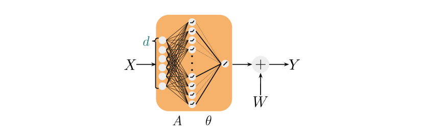
Figure 6: We depict our nonparametric data generating process above. It consists of input dimension $d$, an infinite number of hidden units with ReLU activations, and output dimension $1$. We denote the weights of the first layer via an infinite dimensional matrix $A$ and the weights of the output layer by an infinite dimensional vector $\theta$. To enforce structure which enables learning, we assume an appropriate prior distribution which results in a concentration of the weights of $\theta$ as depicted by the solid (as opposed to dotted) lines in the above diagram. We assume that the final output $Y$ is the sum of the final network output and independent Gaussian noise $Z$.

In this section, we study a nonparameteric data generating process which can be parameterized by a two-layer neural network of infinite width. While the results we present in this section are limited to a two-layer example, the techniques derived in this section are general enough to be applied to appropriate instances of nonparameteric deep neural networks as well.

6.5.1 Data Generating Process

For a nonparametric neural network, we are interested in estimating a function which can be uniquely identified by an infinite-dimensional matrix $A\in\Re^{\infty\times d}$ which represents the first-layer weights, and an infinite-dimensional vector $\theta\in\Re^{\infty}$ which denotes the output-layer weights. As in prior examples, we assume a known prior distribution $\mathbb{P}((A,\theta)\in\cdot)$. The neural network has input dimension $d$ and output dimension $1$. In this analysis, we restrict our attention to a particular prior distribution on the weights of the network. This prior distribution is describe by a Dirichlet process which detail next.

A Dirichlet process is a stochastic process whose realizations are probability mass functions over a countable (often infinite) support. The Dirichlet process takes as input a scale parameter $K$, and a base distribution $P$. Its realizations are hence probability mass functions with support on a countable subset of the set defined by the base distribution $P$. In our problem, we will take this base distribution to be $\text{Unif}(\mathbb{S}^{d-1})$, the uniform distribution over the unit sphere of dimension $d$. As a result, realizations of the Dirichlet process will be probability mass functions over a countable subset of $\mathbb{S}^{d-1}$.

As such, a realization of a Dirichlet process exhibits a parameterization via a vector in $\bar{\theta}\in\Re^{\infty}$ which denotes the frequencies of each outcome along with the collection of vectors in $A_{n}\in\mathbb{S}^{d-1}$ for $n\in\mathbb{Z}_{++}$, which comprise of the support. With this parameterization, we can construct the following data generating process. For all $t$, let $X_{t}\overset{iid}{\sim}\mathcal{N}(0,I_{d})$ and

$$Y_{t+1}=W_{t+1}+\sqrt{K}\cdot\sum_{n=1}^{\infty}\theta_{n}\mathrm{ReLU}(A_{n}^{\top}X_{t}),$$

$$\theta_{n}=\begin{cases}\bar{\theta}_{n}&\text{ w.p. }0.5\\ -\bar{\theta}_{n}&\text{ w.p. }0.5\\ \end{cases},$$

where $\bar{\theta}_{n}$ denotes the frequency associated with the outcome denoted by $A_{n}$ and for all $t$, $W_{t}\overset{iid}{\sim}\mathcal{N}(0,\sigma^{2})$ denotes independent additive Gaussian noise of known variance $\sigma^{2}$.

We now speak about the scale parameter $K$. Evidently, $\bar{\theta}$, though in $\Re^{\infty}$, is limited in complexity by the fact that for all $n$, $\bar{\theta}_{n}\geq 0$ and $\sum_{n=1}^{\infty}\bar{\theta}_{n}=1$. The scale parameter $K$ induces additional structure in the form of concentration. The Dirichlet process inherently assumes a degree of concentration from the fact that its realizations are in a countable subset of $\mathbb{S}^{d-1}$. However, the scale parameter induces further concentration to create a sparsity-like structure in the outcomes. Without such structure, effective learning in the presence of finite compute and memory may be infeasible. Therefore, despite the fact that this neural network is parameterized by an infinite number of parameters, the structure induced by Dirichlet prior and finite scale parameter $K$ will allow us to reason about the achievable performance of an optimal learning algorithm.

6.5.2 Theoretical Building Blocks

In prior sections, we often derived the appropriate rate-distortion result by simply devising a compression which adds independent Gaussian noise to the parameters. This will no longer suffice as the parameters of interest are infinite-dimensional and would hence result in an infinite rate. We introduce a proof technique derived from early results by Barron [1993] in his seminal work on the approximation rates of neural networks. The key insight is that if one samples $m$ times from the categorical distribution induced by $\bar{\theta},A$ and simply construct a function which averages the observed outcomes, the approximation error (in our case, distortion) would decay linearly in $m$. The following theoretical result concretely establishes this idea.

Lemma 32.

(approximation via multinomial) For all $K,m\in\mathbb{Z}_{++},$ let $(A,\bar{\theta})\sim\mathcal{D}\mathcal{P}(K,{\rm Unif}(\mathbb{S}^{d-1}))$ and for all $n\in\mathbb{Z}_{++}$,

$$\theta_{n}=\begin{cases}\bar{\theta}_{n}&\text{ w.p. }0.5\\ -\bar{\theta}_{n}&\text{ w.p. }0.5\\ \end{cases}.$$

If for all $i\in[m]$, $c_{i}\overset{iid}{\sim}{\rm Categorical}(\bar{\theta})$ and $\tilde{A}_{i}=A_{c_{i}}$, then

$$\mathbb{E}\left[\left(\underbrace{\sqrt{K}\cdot\sum_{n=1}^{\infty}\theta_{n}\mathrm{ReLU}(A_{n}^{\top}X_{t})}_{\rm true\ function}-\underbrace{\frac{\sqrt{K}}{m}\sum_{i=1}^{m}{\rm sign}(\theta_{c_{i}})\cdot\mathrm{ReLU}(\tilde{A}_{i}^{\top}X_{t})}_{\rm approximation}\right)^{2}\right]\ \leq\ \frac{K}{m}.$$

Proof.

$$\quad\mathbb{E}\left[\left(\sqrt{K}\cdot\sum_{n=1}^{\infty}\theta_{n}\mathrm{ReLU}(A_{n}^{\top}X_{t})-\frac{\sqrt{K}}{m}\sum_{i=1}^{m}{\rm sign}(\theta_{c_{i}})\cdot\mathrm{ReLU}(\tilde{A}_{i}^{\top}X_{t})\right)^{2}\right]$$

$$\overset{(a)}{=}\mathbb{E}\left[\left(\frac{\sqrt{K}}{m}\sum_{i=1}^{m}{\rm sign}(\theta_{c_{i}})\cdot\mathrm{ReLU}(\tilde{A}_{i}^{\top}X_{t})\right)^{2}-\left(\sqrt{K}\cdot\sum_{n=1}^{\infty}\theta_{n}\mathrm{ReLU}(A_{n}^{\top}X_{t})\right)^{2}\right]$$

$$\leq\mathbb{E}\left[\left(\frac{\sqrt{K}}{m}\sum_{i=1}^{m}{\rm sign}(\theta_{c_{i}})\cdot\mathrm{ReLU}(\tilde{A}_{i}^{\top}X_{t})\right)^{2}\right]$$

$$\overset{(b)}{=}\frac{K}{m^{2}}\sum_{i=1}^{m}\mathbb{E}\left[(\mathrm{ReLU}(\tilde{A}_{i}^{\top}X_{t}))^{2}\right]$$

$$\leq\frac{K}{m^{2}}\sum_{i=1}^{m}\mathbb{E}\left[(\tilde{A}_{i}^{\top}X_{t})^{2}\right]$$

$$=\frac{K}{m},$$

where $(a)$ follows from the fact that the two expressions in the difference have the same expectation and $(b)$ follows from the fact that the $c_{i}$’s are independent and $\mathbb{E}[{\rm sign}(\theta_{c_{i}})]=0$. ∎

This result establishes that despite the fact that this data generating process ostensibly has infinite complexity, there exist good approximations which only require finite information about the data generating process. The above result will allow us to establish bounds on the distortion of a suitable compression. The following result will allow us to establish favorable bounds on the rate of the compression.

Lemma 33.

(Dirichlet-multinomial concentration) For all $K,m\in\mathbb{Z}_{++}$, let $(A,\bar{\theta})\sim\mathcal{D}\mathcal{P}(K,{\rm Unif}(\mathbb{S}^{d-1}))$. If for all $i\in[m]$, $c_{i}\overset{iid}{\sim}{\rm Categorical}(\bar{\theta})$ and $N_{m}$ denotes the random variable which represents the number of unique categories draw in $(c_{1},\ldots,c_{m})$, then

$$\mathbb{E}\left[N_{m}\right]\ \leq\ K\ln\left(1+\frac{n}{K}\right).$$

Proof.

As the proof of this result requires significant mathematical machinery, we refer the reader to Appendix B for the result. ∎

Lemma 33 establishes that the approximation studied above also has favorable informational complexity. Suppose we construct a compression of $(\theta,A)$ as in the statement of Lemma 32, however, instead of setting $\tilde{A}_{i}=A_{c_{i}}$, we instead use a quantization of $\mathbb{S}^{d-1}$. Let $\mathcal{A}_{\epsilon}$ denote an $\epsilon$-cover of $\mathbb{S}^{d-1}$ with respect to $\|\cdot\|^{2}_{2}$. Furthermore, let

$$\bar{A}_{i,\epsilon}=\operatorname*{arg\,min}_{a\in\mathcal{A}_{\epsilon}}\ \|A_{i}-a\|^{2}_{2}.$$

Suppose we construct a compression for which $\tilde{A}_{i}=\bar{A}_{c_{i},\epsilon}$. Then, the collection $(\tilde{A}_{1},\ldots,\tilde{A}_{m})$ will have finite entropy since it consists of a finite collection of discrete random variables defined on the finite set $\mathcal{A}_{\epsilon}$. However, a naive calculation of the entropy will result in a sub-optimal bound on the rate. We arrive at a tighter bound by considering a loss-less compression of $(\tilde{A}_{1},\ldots,\tilde{A}_{m})$ and leveraging the insight of Theorem 3 that entropy is upper bounded by the average length of an optimal prefix-free code.

Theorem 34.

(Dirichlet process rate-distortion upper bound) For all $d,K\in\mathbb{Z}_{++}$ and $\sigma^{2},\epsilon\in\Re_{++}$, if $(X,Y)$ are generated according to the Dirichlet neural network process with parameters $\theta,A$, then

$$\mathbb{H}_{\epsilon}(\theta,A)\ \leq\ K\ln\left(1+\frac{2}{\sigma^{2}\epsilon}\right)\ln\left(\frac{2K}{\sigma^{2}\epsilon}\right)+2dK\ln\left(1+\frac{2}{\sigma^{2}\epsilon}\right)\ln\left(1+\frac{4}{\epsilon}\right).$$

Proof.

Suppose we set $\epsilon^{\prime}=m\sigma^{2}(e^{2K/(m\sigma^{2})}-1)/2K-1\geq 0$ and $m=\lceil\frac{K}{\sigma^{2}\epsilon}\rceil$. For all $i\in[m]$, let $c_{i}\overset{iid}{\sim}{\rm Categorical}(\bar{\theta})$. Let $\mathcal{A}_{\epsilon}$ denote an $\epsilon^{\prime}$-cover of $\mathbb{S}^{d-1}$ with respect to $\|\cdot\|^{2}_{2}$ and for all $i\in\mathbb{Z}_{++}$, let

$$\bar{A}_{i,\epsilon}=\operatorname*{arg\,min}_{a\in\mathcal{A}_{\epsilon}}\ \|A_{i}-a\|^{2}_{2}.$$

Recall that $N_{m}$ denotes the number of unique outcomes in $(c_{1},\ldots,c_{m})$. Let $\mathcal{I}=(I_{1},\ldots,I_{N_{m}})$ denote an ordered set which consists of the unique outcomes. Let $(\tilde{\theta},\tilde{A})=(\tilde{\theta}_{1},\tilde{A}_{1},\ldots,\tilde{\theta}_{N_{m}},\tilde{A}_{N_{m}})$ be a collection of random variable such that

$$\tilde{A}_{i}=\bar{A}_{I_{i},\epsilon};\quad\tilde{\theta}_{i}=\sum_{j=1}^{m}{\rm sign}(\theta_{I_{i}})\cdot\mathbbm{1}[c_{j}=I_{i}].$$

Therefore, $\tilde{\theta}$ consists of $N_{m}$ integers in $\pm[m]$ and $\tilde{A}$ consists of $N_{m}$ outcomes from the set $\mathcal{A}_{\epsilon}$. We begin by upper bounding the distortion of $(\tilde{\theta},\tilde{A})$.

$$\mathbb{I}(Y;\theta,A|\tilde{\theta},\tilde{A},X) =\mathbf{h}(Y|\tilde{\theta},\tilde{A},X)-\mathbf{h}(Y|\theta,A)$$

$$=\mathbf{h}\left(Y-\frac{\sqrt{K}}{m}\sum_{i\in\mathcal{I}}\tilde{\theta}_{i}\cdot\mathrm{ReLU}(\tilde{A}_{i}^{\top}X)\bigg{|}\tilde{\theta},\tilde{A}\right)-\mathbf{h}(W)$$

$$\overset{(a)}{\leq}\mathbb{E}\left[\frac{1}{2}\ln\left(\frac{\left(Y-\frac{\sqrt{K}}{m}\sum_{i\in\mathcal{I}}\tilde{\theta}_{i}\cdot\mathrm{ReLU}(\tilde{A}_{i}^{\top}X)\right)^{2}}{\sigma^{2}}\right)\right]$$

$$\overset{(b)}{\leq}\frac{1}{2}\ln\left(\frac{\mathbb{E}\left[\left(Y-\frac{\sqrt{K}}{m}\sum_{i\in\mathcal{I}}\tilde{\theta}_{i}\cdot\mathrm{ReLU}(\tilde{A}_{i}^{\top}X)\right)^{2}\right]}{\sigma^{2}}\right)$$

$$=\frac{1}{2}\ln\left(1+\frac{\left(\sqrt{K}\cdot\sum_{n=1}^{\infty}\theta_{n}\mathrm{ReLU}(A_{n}^{\top}X)-\frac{\sqrt{K}}{m}\sum_{i=1}^{m}{\rm sign}(\theta_{c_{i}})\cdot\mathrm{ReLU}(\tilde{A}_{i}^{\top}X)\right)^{2}}{\sigma^{2}}\right)$$

$$\overset{(c)}{\leq}\frac{1}{2}\ln\left(1+\frac{\frac{2K}{m}+\frac{2K}{m^{2}}\mathbb{E}\left[\left(\sum_{i=1}^{m}{\rm sign}(\theta_{c_{i}})\mathrm{ReLU}(A_{i}^{\top}X)-\sum_{i=1}^{m}{\rm sign}(\theta_{c_{i}})\cdot\mathrm{ReLU}(\tilde{A}_{i}^{\top}X)\right)^{2}\right]}{\sigma^{2}}\right)$$

$$=\frac{1}{2}\ln\left(1+\frac{\frac{2K}{m}+\frac{2K}{m^{2}}\sum_{i=1}^{m}\mathbb{E}\left[(\mathrm{ReLU}(A^{\top}_{i}X)-\mathrm{ReLU}(\tilde{A}_{i}^{\top}X))^{2}\right]}{\sigma^{2}}\right)$$

$$\overset{(d)}{\leq}\frac{1}{2}\ln\left(1+\frac{\frac{2K}{m}+\frac{2K}{m}\mathbb{E}\left[(A^{\top}_{i}X-\tilde{A}_{i}^{\top}X)^{2}\right]}{\sigma^{2}}\right)$$

$$\overset{(e)}{\leq}\frac{1}{2}\ln\left(1+\frac{2K(1+\epsilon^{\prime})}{\sigma^{2}m}\right)$$

$$=\frac{K}{\sigma^{2}m}$$

$$\leq\epsilon,$$

where $(a)$ follows from Theorem 11 and the fact that conditioning reduces differential entropy, $(b)$ follows from Jensen’s inequality, $(c)$ follows from Lemma 32 and the fact that for all $x,y,z\in\Re$, $(x-y)^{2}\leq 2(x-z)^{2}+2(z-y)^{2}$, $(d)$ follows from the fact that for all $x,y\in\Re,\ (x-y)^{2}\geq(\mathrm{ReLU}(x)-\mathrm{ReLU}(y))^{2}$, and $(e)$ follows from the fact that $\tilde{A}_{i}$ is the closest element in an $\epsilon^{\prime}$ cover of $\mathbb{S}^{d-1}$.

We now upper bound the rate of $(\tilde{\theta},\tilde{A})$

$$\mathbb{I}(\theta,A;\tilde{\theta},\tilde{A}) \leq\mathbb{H}(\tilde{\theta},\tilde{A})$$

$$\overset{(a)}{\leq}\mathbb{E}\left[N_{m}\cdot\left(\ln(2m)+\ln(|\mathcal{A}_{\epsilon^{\prime}}|)\right)\right]$$

$$\overset{(b)}{\leq}K\ln\left(1+\frac{m}{K}\right)\left(\ln 2m+d\ln\frac{3}{{\epsilon^{\prime}}^{2}}\right)$$

$$\overset{(c)}{\leq}K\ln\left(1+\frac{2}{\sigma^{2}\epsilon}\right)\left(\ln\frac{2K}{\sigma^{2}\epsilon}+2d\ln\left(\frac{\epsilon\sqrt{3}}{e^{\epsilon}-1-\epsilon}\right)\right)$$

$$\overset{(d)}{\leq}K\ln\left(1+\frac{2}{\sigma^{2}\epsilon}\right)\ln\left(\frac{2K}{\sigma^{2}\epsilon}\right)+2dK\ln\left(1+\frac{2}{\sigma^{2}\epsilon}\right)\ln\left(1+\frac{4}{\epsilon}\right),$$

where $(a)$ follows from Theorem 3 and the fact that a realization $(\tilde{\theta},\tilde{A})$ can be mapped to a codeword of length $N_{m}(\ln(2m)+\ln(|\mathcal{A}_{\epsilon^{\prime}}|))$ by using $\ln(2m)$ nats to encode each of $\tilde{\theta}_{1},\ldots,\tilde{\theta}_{N_{m}}$, and $\ln(|\mathcal{A}_{\epsilon^{\prime}}|)$ to encode each of $\tilde{A}_{1},\ldots,\tilde{A}_{N_{m}}$, $(b)$ follows from Lemma 33 and the fact that $|\mathcal{A}_{\epsilon^{\prime}}|\leq(3/{\epsilon^{\prime}}^{2})^{d}$, $(c)$ follows by upper bounding the quantity via $m=2K/(\sigma^{2}\epsilon)$ as opposed to $\lceil K/(\sigma^{2}\epsilon)\rceil$, and $(d)$ follows from the fact that for all $\epsilon\geq 0$, $\ln(\epsilon\sqrt{3}/(e^{\epsilon}-1-\epsilon))\leq\ln(1+4/\epsilon)$. ∎

6.5.3 Main Result

With the theoretical tools derived in the previous section, we now establish the following upper bound on the estimation error of an optimal agent learning from data generated by the Dirichlet process.

Theorem 35.

(Dirichlet process estimation error upper bound) For all $d,K\in\mathbb{Z}_{++}$, if for all $t$, $(X_{t},Y_{t+1})$ are generated according to the Dirichlet neural network process, then for all $T$,

$$\mathcal{L}_{T}\ \leq\ \frac{K}{T}\ln\left(1+\frac{T}{\sigma^{2}d}\right)\ln\left(\frac{T}{\sigma^{2}d}\right)+\frac{2dK}{T}\left(1+\ln\left(1+\frac{T}{\sigma^{2}d}\right)\ln\left(1+\frac{T}{dK}\right)\right).$$

Proof.

The result follows from Theorems 15 and 34 and setting $\epsilon=2dk/T$. ∎

Notably, this result is $\tilde{\mathcal{O}}(dK/T)$ despite the fact that the Dirichlet neural network process is described by a neural network with infinite width. The scale parameter $K$ determines the degree of concentration which occurs in the output-layer weights of the network and hence controls the difficult of learning. This example of learning under data generated by a nonparametric process further demonstrates the flexibility and ingenuity of proof techniques which are encompassed in our framework. We hope that the suite of examples provided in this section enables the reader to analyze whichever complex processes they may have in mind.

Summary

• (monotonicity of per-timestep estimation error) If for all $s\in\mathbb{Z}_{+}$, $(X_{s},Y_{s+1})$ is sampled iid from some distribution $\mathbb{P}(\cdot|\theta)$, then for all $t\in\mathbb{Z}_{+}$,

  $$\mathbb{I}(Y_{t+2};\theta|H_{t+1})\ \leq\ \mathbb{I}(Y_{t+1};\theta|H_{t}).$$

• For all $\epsilon\geq 0$, we let

  $$\mathbb{H}_{\epsilon}(\theta)=\inf_{\tilde{\theta}\in\tilde{\Theta}_{\epsilon}}\mathbb{I}(\theta;\tilde{\theta}),$$

  where

  $$\tilde{\Theta}_{\epsilon}=\{\tilde{\theta}:\tilde{\theta}\perp H_{\infty}|\theta,\ \mathbb{I}(Y_{1};\theta|\tilde{\theta},X_{0})\leq\epsilon\}.$$

  Note that in contrast to the general rate-distortion formulation of section 5, this modified rate-distortion does not depend on the time horizon $T$.

• (linear regression estimation error bounds) For all input dimensions $d\in\mathbb{Z}_{++}$ and noise variance $\sigma^{2}\geq 0$, if for all $t$, $(X_{t},Y_{t+1})$ are generated according to the linear regression processes, then for all $T$,

  $$\frac{d}{2T}W\left(\frac{2T}{d(8+\frac{d}{d-2}\sigma^{2})}\right)\ \leq\ \mathcal{L}_{T}\ \leq\ \left(\frac{d}{2T}\ln\left(\frac{T}{\sigma^{2}d}\right)\right)_{+}+\frac{1}{2T}\ln\left(1+\frac{d}{T}\right),$$

  where $W$ is the Lambert W function.

• (logistic regression estimation error upper bound) For all input dimensions $d\in\mathbb{Z}_{++}$, if for all $t$, $(X_{t},Y_{t+1})$ is generated according to the logistic regression process, then for all $T,$

  $$\mathcal{L}_{T}\ \leq\ \frac{d}{2T}\left(1+\ln\left(1+\frac{T}{4d}\right)\right).$$

• (deep neural network estimation error upper bound) For all input dimensions $d$, widths $N$, and depths $L$ each $\in\mathbb{Z}_{++}$, and noise variances $\sigma^{2}\in\Re_{++}$, if for all $t$, $(X_{t},Y_{t+1})$ are generated according to the deep neural network process, then for all $T$,

  $$\mathcal{L}_{T}\ \leq\ \frac{P}{2T}\left(1+\ln\left(1+\frac{2LT}{\sigma^{2}P}\right)\right),$$

  where $P=(L-2)N^{2}+N+dN$ denotes the total parameter count of the network.

• (Dirichlet process estimation error upper bound) For all input dimensions $d$, scale parameters $K$, each $\in\mathbb{Z}_{++}$, if for all $t$, $(X_{t},Y_{t+1})$ are generated according to the Dirichlet neural network process, then for all $T$,

  $$\mathcal{L}_{T}\ \leq\ \frac{K}{T}\ln\left(1+\frac{T}{\sigma^{2}d}\right)\ln\left(\frac{T}{\sigma^{2}d}\right)+\frac{2dK}{T}\left(1+\ln\left(1+\frac{T}{\sigma^{2}d}\right)\ln\left(1+\frac{T}{dK}\right)\right).$$

7 Learning from Sequences

In the previous section, we focused on the special case of learning from an (infintely) exchangeable sequence of data (iid when conditioned on $\theta$). However, in general, machine learning systems will have to reason about data which does not obey this rigid structure. For instance, suppose that $X_{0},X_{1},X_{2},\ldots$ describes a sequence of text tokens from a book. It’s clear that such a sequence would not exhibit exchangeability as the order of the tokens plays a critical role in deriving meaning. Existing frameworks for analyzing machine learning can only reason about learning from sequential data under rigid and contrived notions of mixing time for the data generating process. However, in our framework, Theorem 15 does not make any explicit assumptions on the structure of the data. In this section, we will demonstrate that Theorem 15 seamlessly extends to the analysis of learning from data generated by an auto-regressive process.

7.1 Data Generating Process

Let $X_{0},X_{1},X_{2},$ be a sequence of random variables representing observations. We assume that this sequence is generated by an autoregressive model which is parameterized by a random variable $\theta$. As a result, for all $t$, $X_{t+1}$ is drawn according to a probability distribution which depends on $\theta$ and the history $H_{t}=(X_{0},X_{1},\ldots,X_{t})$. In this section, we will analyze learning under two concrete autoregressive data generating processes. The first involves a binary AR(K) process and the second a transformer model with context length $K$.

7.2 Binary AR(K) Process

7.2.1 Data Generating Process

We begin with a simple AR(K) process over a binary alphabet. We aim to demonstrate that our framework can easily adapt to machine learning from sequential data. In this problem, we are interested in estimating random vectors $\theta_{1},\ldots,\theta_{K}\in\Re^{d}$ from data which is generated in the following way. Let $(X_{0},X_{1}\ldots,X_{K-1})\sim{\rm Unif}(\{0,1\}^{K})$. Furthermore, consider known vectors $\Phi_{0},\Phi_{1}\in\Re^{d}$ of $L2$ norm equal to $1$ which correspond to vector embedding of the binary outcomes $0$ and $1$ respectively. For brevity of notation, we use $\phi_{t}$ to denote $\Phi_{X_{t}}$.

For all $t\geq K$, let

$$X_{t+1}=\begin{cases}1&\text{ w.p. }\sigma\left(\sum_{k=1}^{K}\theta_{k}^{\top}\phi_{t-k+1}\right)\\ 0&\text{ otherwise}\end{cases},$$

where $\sigma$ denotes the sigmoid function. For all $k$, we assume the independent prior distributions $\mathbb{P}(\theta_{k})=\mathcal{N}(0,I_{d}/(K))$.

7.2.2 Preliminary Theoretical Results

As in all prior examples, our strategy is to leverage rate-distortion theory to arrive at an estimation error upper bound. We begin with the following result which upper bounds the rate-distortion function in the binary AR(K) problem setting.

Lemma 36.

(binary AR(K) rate-distortion upper bound) For all $d,K\in\mathbb{Z}_{++}$ and $\epsilon\in\Re_{++}$, if for all $t\in\mathbb{Z}_{+},X_{t}$ is generated according to the binary AR(K) process, then for all $T$,

$$\mathbb{H}_{\epsilon,T}(\theta_{1:K})\ \leq\ \frac{dK}{2}\ln\left(1+\frac{1}{8\epsilon}\right).$$

Proof.

For $k\in\{0,1,\ldots,K-1\}$, let $\tilde{\theta}_{k}=\theta_{k}+Z_{k}$ where $Z_{k}\perp\theta_{k}$ and $Z_{k}\sim\mathcal{N}(0,I_{d}\cdot 8\epsilon/K)$. For all $t$, let $H_{t}$ denote $(X_{0},X_{1},\ldots,X_{t})$. Then,

$$\frac{\mathbb{I}(H_{T};\theta_{1:K}|\tilde{\theta}_{1:K})}{T}$$

$$=\frac{1}{T}\sum_{t=0}^{T-1}\mathbb{I}(X_{t+1};\theta_{1:K}|\tilde{\theta}_{1:K},H_{t})$$

$$\leq\frac{1}{T}\sum_{t=0}^{T-1}\mathbb{I}(X_{t+1};\theta_{1:K}|\tilde{\theta}_{1:K},X_{t:t-K+1})$$

$$\leq\frac{1}{T}\sum_{t=0}^{T-1}\mathbb{E}\left[{\mathbf{d}}_{\rm KL}\left(\mathbb{P}(X_{t+1}\in\cdot|\theta_{1:K},X_{t:t-K+1})\ \|\ \mathbb{P}(X_{t+1}\in\cdot|\tilde{\theta}_{1:K},X_{t:t-K+1})\right)\right]$$

$$\overset{(a)}{\leq}\frac{1}{T}\sum_{t=0}^{T-1}\mathbb{E}\left[{\mathbf{d}}_{\rm KL}\left(\mathbb{P}(X_{t+1}\in\cdot|\theta_{1:K},X_{t:t-K+1})\ \|\ \mathbb{P}(X_{t+1}\in\cdot|\theta_{1:K}\leftarrow\tilde{\theta}_{1:K},X_{t:t-K+1})\right)\right]$$

$$=\frac{1}{T}\sum_{t=0}^{T-1}\mathbb{E}\left[\frac{\ln\left(\frac{1+e^{-\sum_{k=1}^{K}\theta_{k}^{\top}\phi_{t-k+1}}}{1+e^{-\sum_{k=1}^{K}\theta_{k}^{\top}\phi_{t-k+1}}}\right)}{1+e^{-\sum_{k=1}^{K}\theta_{k}^{\top}\phi_{t-k+1}}}+\frac{\ln\left(\frac{1+e^{\sum_{k=1}^{K}\theta_{k}^{\top}\phi_{t-k+1}}}{1+e^{\sum_{k=1}^{K}\theta_{k}^{\top}\phi_{t-k+1}}}\right)}{1+e^{\sum_{k=1}^{K}\theta_{k}^{\top}\phi_{t-k+1}}}\right]$$

$$\overset{(b)}{\leq}\frac{1}{T}\sum_{t=0}^{T-1}\frac{\mathbb{E}\left[\left(\sum_{k=1}^{K}\theta_{k}^{\top}\phi_{t-k+1}-\tilde{\theta}^{\top}_{k}\phi_{t-k+1}\right)^{2}\right]}{8}$$

$$=\frac{1}{T}\sum_{t=0}^{T-1}\frac{\mathbb{E}\left[\sum_{k=1}^{K}\phi_{t:t-K+1}^{\top}(\theta_{k}-\tilde{\theta}_{k})(\theta_{k}-\tilde{\theta}_{k})^{\top}\phi_{t:t-K+1}\right]}{8}$$

$$=\frac{\epsilon\cdot\mathbb{E}\left[\sum_{k=1}^{K}\phi^{\top}_{t-k}\phi_{t-k+1}\right]}{K}$$

$$=\epsilon,$$

where $(a)$ follows from Lemma 57 and $(b)$ follows from Lemma 23.

We now upper bound the rate.

$$\mathbb{I}(\theta_{1:K};\tilde{\theta}_{1:K}) =\mathbf{h}(\tilde{\theta}_{1:K})-\mathbf{h}(\tilde{\theta}_{1:K}|\theta_{1:K})$$

$$\overset{(a)}{\leq}\frac{dK}{2}\ln\left(2\pi e\left(\frac{1}{K}+\frac{8\epsilon}{K}\right)\right)-\frac{dK}{2}\ln\left(2\pi e\frac{8\epsilon}{K}\right)$$

$$=\frac{dK}{2}\ln\left(1+\frac{1}{8\epsilon}\right),$$

where $(a)$ follows from Lemma 11. The result follows. ∎

7.2.3 Main Result

We now present the main result of this section which upper bounds the estimation error of learning under the binary AR(K) data generating process. The result follows directly as a result of Lemma 36.

Theorem 37.

(binary AR(K) estimation error upper bound) For all $d,K\in\mathbb{Z}_{++}$, if for all $t\in\mathbb{Z}_{+},X_{t}$ is generated according to the binary AR(K) process, then for all $T$,

$$\mathcal{L}_{T}\ \leq\ \frac{dK}{2T}\left(1+\ln\left(1+\frac{T}{4dK}\right)\right).$$

Proof.

$$\mathcal{L}_{T} \overset{(a)}{\leq}\inf_{\epsilon\geq 0}\frac{\mathbb{H}_{\epsilon,T}(\theta_{1:K})}{T}+\epsilon$$

$$\overset{(b)}{\leq}\inf_{\epsilon\geq 0}\frac{dK\ln\left(1+\frac{1}{8\epsilon}\right)}{2T}+\epsilon$$

$$\overset{(c)}{\leq}\frac{dK}{2T}\left(1+\ln\left(1+\frac{T}{4dK}\right)\right),$$

where $(a)$ follows from Theorem 15, $(b)$ follows from Lemma 36, and $(c)$ follows by setting $\epsilon=(dK)/(2T)$. ∎

An interesting aspect of this result is that both the proof techniques and final result are hardly impacted by the fact that the sequence is not iid when conditioned on $\theta_{1:K}$. Existing tools for statistical analysis can struggle in the setting without the appropriate averages of iid quantities. However, our analytical tools involving rate-distortion theory allow us to handle such problem instances with relative ease and produce reasonable upper bounds on estimation error in learning settings involving sequences of data. In the following section, we extend these tools to analyze a more complex transformer data generating process.

7.3 Transformer Process

7.3.1 Data Generating Process

Let $X_{0},X_{2},\ldots$ be a sequence over a finite vocabulary $\{1,\ldots,d\}$. Each of the $d$ outcomes is associated with a known embedding vector denoted as $\Phi_{j}$ for $j\in\{1,\ldots,d\}$. We assume that for all $j$, $\|\Phi_{j}\|_{2}=1$. For brevity of notation, we let $\phi_{t}=\Phi_{X_{t}}$ i.e. the embedding associated with token $X_{t}$.

Let $K$ denote the context length of the transformer, $L$ denote it’s depth, and $r$ denote the attention dimension. We assume that the first token $X_{0}$ is sampled from an arbitrary pmf on $\{1,\ldots,d\}$ but subsequent tokens are sampled based on the previous $K$ tokens within the context window and the weights of a depth $L$ transformer model.

Just as in the deep neural networks section, we use $U_{t}^{(\ell)}$ to denote the output of layer $\ell$ at time $t$. As a result, for $\ell=0$, $U_{t,0}=\phi_{t-K+1:t}$ (the embeddings associated with the past $K$ tokens). For all $t\leq T,\ell<L$, let

$$\text{Attn}^{(\ell)}\left(U_{t}^{(\ell-1)}\right)={\rm Softmax}\left(\frac{U^{(\ell-1)\top}_{t}A^{(\ell)}U_{t}^{(\ell-1)}}{\sqrt{r}}\right)$$

denote the attention matrix of layer $(\ell)$ where ${\rm Softmax}$ denotes the softmax function applied elementwise along the columns. The matrix $A^{(\ell)}\in\Re^{r\times r}$ can be interpreted as the product of the key and query matrices and without loss of generality, we assume that the elements of the matrices $A^{(\ell)}$ are distributed iid $\mathcal{N}(0,1)$ (Gaussian assumption is not crucial but unit variance is).

Subsequently, we let

$$U_{t}^{(\ell)}=\text{Clip}\left(V^{(\ell)}U_{t}^{(\ell-1)}\text{Attn}^{(\ell)}\left(U_{t}^{(\ell-1)}\right)\right),$$

where Clip ensures that each column of the matrix input has $L_{2}$ norm at most $1$. The matrix $V^{(\ell)}$ resembles the value matrix and we assume that the rows of $V^{(\ell)}$ are distributed iid ${\rm Unif}(\mathbb{S}^{d-1})$. For $\ell<L$, we have that $V^{(\ell)}\in\Re^{r\times r}$, whereas $V^{(L)}\in\Re^{d\times r}$.

Finally, the next token is generated via sampling from the softmax of the final layer:

$$X_{t+1}\sim{\rm Softmax}\left(U_{t}^{(L)}[-1]\right),$$

where $U_{t}^{(L)}[-1]$ denotes the right-most column of $U_{t}^{(L)}$. At each layer $\ell$, the parameters $\theta^{(\ell)}$ consist of the matrices $A^{(\ell)},V^{(\ell)}$.

7.3.2 Theoretical Building Blocks

As with deep neural networks, our strategy is to drive a rate-distortion bound by deriving a suitable bound for the distortion function. Recall that by the chain rule, for all $t$,

$$\mathbb{I}(X_{t+1};\theta^{(1:L)}|\tilde{\theta}^{(1:L)},H_{t})\ =\ \sum_{\ell=1}^{L}\mathbb{I}(X_{t+1};\theta^{(\ell)}|\theta^{(\ell+1:L)},\tilde{\theta}^{(1:\ell)},H_{t}).$$

In the deep neural network setting, the above RHS could be further simplified via an upper bound which replaces the conditioning on $\tilde{\theta}^{(1:\ell)}$ to $(\tilde{\theta}^{(\ell)},\theta^{(1:\ell-1)})$. However, this result relied heavily on the iid structure of the data. In the sequential data setting, we have the following weaker result which still facilitates our analysis.

Lemma 38.

For all $t,L\in\mathbb{Z}_{++}$ and $\ell\in\{1,\ldots,L\}$, if $\theta^{(i)}\perp\theta^{(j)}$, $\tilde{\theta}^{(i)}\perp\tilde{\theta}^{(j)}$, and $\theta^{(i)}\perp\tilde{\theta}^{(j)}$ for $i\neq j$, then

$$\mathbb{I}(X_{t+1};\theta^{(\ell)}|\theta^{(\ell+1:L)},\tilde{\theta}^{(1:\ell)},H_{t})\ \leq\ \mathbb{I}(H_{t+1};\theta^{(\ell)}|\theta^{(\ell+1:L)},\theta^{(1:\ell-1)},\tilde{\theta}^{(\ell)},X_{0}).$$

Proof.

$$\mathbb{I}(X_{t+1};\theta^{(\ell)}|\theta^{(\ell+1:L)},\tilde{\theta}^{(1:\ell)},H_{t}) \overset{(a)}{=}\mathbb{I}(H_{t+1},\tilde{\theta}^{(1:\ell-1)};\theta^{(\ell)}|\theta^{(\ell+1:L)},\tilde{\theta}^{(\ell)})-\mathbb{I}(H_{t},\tilde{\theta}^{(1:\ell-1)};\theta^{(\ell)}|\theta^{(\ell+1:L)},\tilde{\theta}^{(\ell)})$$

$$\overset{(b)}{\leq}\mathbb{I}(H_{t+1},\tilde{\theta}^{(1:\ell-1)};\theta^{(\ell)}|\theta^{(\ell+1:L)},\tilde{\theta}^{(\ell)},X_{0})$$

$$\overset{(c)}{\leq}\mathbb{I}(H_{t+1},\theta^{(1:\ell-1)};\theta^{(\ell)}|\theta^{(\ell+1:L)},\tilde{\theta}^{(\ell)},X_{0})$$

$$\overset{(d)}{=}\mathbb{I}(H_{t+1},\theta^{(1:\ell-1)};\theta^{(\ell)}|\theta^{(\ell+1:L)},\tilde{\theta}^{(\ell)},X_{0})-\mathbb{I}(\theta^{(1:\ell-1)};\theta^{(\ell)}|\theta^{(\ell+1:L)},\tilde{\theta}^{(\ell)},X_{0})$$

$$\overset{(e)}{=}\mathbb{I}(H_{t+1};\theta^{(\ell)}|\theta^{(\ell+1:L)},\theta^{(1:\ell-1)},\tilde{\theta}^{(\ell)},X_{0})$$

where $(a)$ follows from the chain rule of mutual information, $(b)$ follows from the independence assumptions, $(c)$ follows from the data processing inequality applied to the markov chain $\theta_{i}\perp\tilde{\theta}^{(1:\ell-1)}|(H_{t+1},\theta^{(\ell+1:L)},\theta^{(1:\ell-1)},X_{0}^{K})$, $(d)$ follows from the fact that $\mathbb{I}(\theta^{(1:\ell-1)};\theta_{i}|\theta^{(\ell+1:L)},\tilde{\theta}_{i},X_{0})=0$, and $(e)$ follows from the chain rule of mutual information. ∎

Note that in the RHS of Lemma 38 is $H_{t+1}$ as opposed to $X_{t+1}$ which we would have desired. Nonetheless, this factor of $t$ will eventually only appear as a logarithmic factor in the final bound. To account for the influence of conditioning on the future layers $\theta^{(\ell+1:L)}$, we establish the following result on the squared Lipschitz constant. Note that we use $\|\cdot\|_{\sigma}$ to denote the operator norm of a matrix and $\|\cdot\|_{F}$ to denote the frobenius norm.

Lemma 39.

(transformer layer Lipschitz) For all $d,r,K,\ell\in\mathbb{Z}_{++}$, if

$$\tilde{U}^{(\ell)}={\rm Clip}\left(V^{(\ell)}\tilde{U}^{(\ell-1)}{\rm Attn}^{(\ell)}\left(\tilde{U}^{(\ell-1)}\right)\right),$$

then

$$\left\|U^{(\ell)}-\tilde{U}^{(\ell)}\right\|^{2}_{F}\ \leq\ 2K\|V^{(\ell)}\|^{2}_{\sigma}\left(1+\frac{4K\|A^{(\ell)}\|^{2}_{\sigma}}{r}\right)\cdot\left\|U^{(\ell-1)}-\tilde{U}^{(\ell-1)}\right\|^{2}_{F}.$$

Proof.

$$\ \left\|U^{(\ell)}-\tilde{U}^{(\ell)}\right\|^{2}_{F}$$

$$=\left\|\text{Clip}\left(V^{(\ell)}U^{(\ell-1)}\sigma\left(\frac{U^{(\ell-1)\top}A^{(\ell)}U^{(\ell-1)}}{\sqrt{r}}\right)\right)-\text{Clip}\left(V^{(\ell)}\tilde{U}^{(\ell-1)}\sigma\left(\frac{\tilde{U}^{(\ell-1)\top}A^{(\ell)}\tilde{U}^{(\ell-1)}}{\sqrt{r}}\right)\right)\right\|^{2}_{F}$$

$$\overset{(a)}{\leq}\left\|V^{(\ell)}U^{(\ell-1)}\sigma\left(\frac{U^{(\ell-1)\top}A^{(\ell)}U^{(\ell-1)}}{\sqrt{r}}\right)-V^{(\ell)}\tilde{U}^{(\ell-1)}\sigma\left(\frac{\tilde{U}^{(\ell-1)\top}A^{(\ell)}\tilde{U}^{(\ell-1)}}{\sqrt{r}}\right)\right\|^{2}_{F}$$

$$\overset{(b)}{=}\sum_{k=1}^{K}\|V^{(\ell)}\|^{2}_{\sigma}\left\|U^{(\ell-1)}\sigma\left(\frac{U^{(\ell-1)\top}A^{(\ell)}U^{(\ell-1)}_{k}}{\sqrt{r}}\right)-\tilde{U}^{(\ell-1)}\sigma\left(\frac{\tilde{U}^{(\ell-1)\top}A^{(\ell)}\tilde{U}^{(\ell-1)}_{k}}{\sqrt{r}}\right)\right\|^{2}_{2}$$

$$\leq\sum_{k=1}^{K}2\|V^{(\ell)}\|^{2}_{\sigma}\left\|U^{(\ell-1)}\sigma\left(\frac{U^{(\ell-1)\top}A^{(\ell)}U^{(\ell-1)}_{k}}{\sqrt{r}}\right)-\tilde{U}^{(\ell-1)}\sigma\left(\frac{U^{(\ell-1)\top}A^{(\ell)}U^{(\ell-1)}_{k}}{\sqrt{r}}\right)\right\|^{2}_{2}$$

$$\quad+\sum_{k=1}^{K}2\|V^{(\ell)}\|^{2}_{\sigma}\left\|\tilde{U}^{(\ell-1)}\sigma\left(\frac{U^{(\ell-1)\top}A^{(\ell)}U^{(\ell-1)}_{k}}{\sqrt{r}}\right)-\tilde{U}^{(\ell-1)}\sigma\left(\frac{\tilde{U}^{(\ell-1)\top}A^{(\ell)}\tilde{U}^{(\ell-1)}_{k}}{\sqrt{r}}\right)\right\|^{2}_{2}$$

$$\overset{(c)}{\leq}\sum_{k=1}^{K}2\|V^{(\ell)}\|^{2}_{\sigma}\|U^{(\ell-1)}-\tilde{U}^{(\ell-1)}\|^{2}_{F}$$

$$\quad+\sum_{k=1}^{K}\frac{2K}{r}\|V^{(\ell)}\|^{2}_{\sigma}\left\|U^{(\ell-1)\top}A^{(\ell)}U^{(\ell-1)}_{k}-\tilde{U}^{(\ell-1)\top}A^{(\ell)}\tilde{U}^{(\ell-1)}_{k}\right\|^{2}_{2}$$

$$\overset{(d)}{\leq}2K\|V^{(\ell)}\|^{2}_{\sigma}\left\|U^{(\ell-1)}-\tilde{U}^{(\ell-1)}\right\|^{2}_{F}+\frac{4K}{r}\sum_{k=1}^{K}\|V^{(\ell)}\|^{2}_{\sigma}\left\|U^{(\ell-1)\top}A^{(\ell)}U^{(\ell-1)}_{k}-U^{(\ell-1)\top}A^{(\ell)}\tilde{U}^{(\ell-1)}_{k}\right\|^{2}_{2}$$

$$\quad+\frac{4K}{r}\sum_{k=1}^{K}\|V^{(\ell)}\|^{2}_{\sigma}\left\|U^{(\ell-1)\top}A^{(\ell)}\tilde{U}^{(\ell-1)}_{k}-\tilde{U}^{(\ell-1)\top}A^{(\ell)}\tilde{U}^{(\ell-1)}_{k}\right\|^{2}_{2}$$

$$\overset{(e)}{\leq}2K\|V^{(\ell)}\|^{2}_{\sigma}\left\|U^{(\ell-1)}-\tilde{U}^{(\ell-1)}\right\|^{2}_{F}+\frac{4K^{2}}{r}\sum_{k=1}^{K}\|V^{(\ell)}\|^{2}_{\sigma}\|A^{(\ell)}\|^{2}_{\sigma}\left\|U^{(\ell-1)}_{k}-\tilde{U}^{(\ell-1)}_{k}\right\|^{2}_{2}$$

$$\quad+\frac{4K}{r}\sum_{k=1}^{K}\|V^{(\ell)}\|^{2}_{\sigma}\|A^{(\ell)}\|^{2}_{\sigma}\left\|U^{(\ell-1)}-\tilde{U}^{(\ell-1)}\right\|^{2}_{F}$$

$$=2K\|V^{(\ell)}\|^{2}_{\sigma}\left\|U^{(\ell-1)}-\tilde{U}^{(\ell-1)}\right\|^{2}_{F}+\frac{8K^{2}}{r}\|V^{(\ell)}\|^{2}_{\sigma}\|A^{(\ell)}\|^{2}_{\sigma}\left\|U^{(\ell-1)}-\tilde{U}^{(\ell-1)}\right\|^{2}_{F}$$

$$=2K\|V^{(\ell)}\|^{2}_{\sigma}\left(1+\frac{4K\|A^{(\ell)}\|^{2}_{\sigma}}{r}\right)\cdot\left\|U^{(\ell-1)}-\tilde{U}^{(\ell-1)}\right\|^{2}_{F},$$

where $(a)$ follows from the fact that Clip is a contraction mapping, where in $(b)$, $U^{(\ell-1)}_{k}$ denotes the $k$th column of $U^{(\ell-1)}\in\Re^{d\times K}$, $(c)$ follows from the fact $\|\tilde{U}^{(\ell-1)}\|^{2}_{\sigma}\leq K$ and the fact that softmax is $1$-Lipschitz, $(d)$ follows from the fact that $(x+z)^{2}\leq 2(x-y)^{2}+2(y+z)^{2}$, and $(e)$ follows from the fact that $\|U^{(\ell-1)}U^{(\ell-1)\top}\|_{\sigma}\leq K$. ∎

note that again, unlike the standard deep neural network setting, the Lipschitz constant is not $1$, but rather scales with $K$, the context length. The intricacies of the softmax self-attention mechanism complicate the process of arriving at a tight characterization. However, for the purposes of deriving an estimation error bound, this result will suffice.

With this result in place, we now upper bound the expected squared difference between an output generated by a transformer layer with the correct weights $A,V$ and an output generated by slightly perturbed weights $\tilde{A},\tilde{V}$.

Lemma 40.

For all $d,r,K\in\mathbb{Z}_{++}$ and $\epsilon\geq 0$, if $V\in\Re^{r\times r}$ consists of elements distributed iid $\mathcal{N}(0,1/r)$, $A\in\Re^{r\times r}$ consists of elements distributed $\mathcal{N}(0,1)$, for all $\ell\in[L]$,

$$\tilde{U}^{(\ell)}={\rm Clip}\left(\tilde{V}^{(\ell)}U^{(\ell-1)}\tilde{{\rm Attn}}^{(\ell)}\left(U^{(\ell-1)}\right)\right),$$

where for all $\ell<L$, $\mathbb{E}[\|V^{(\ell)}-\tilde{V}^{(\ell)}\|^{2}_{F}]\leq\epsilon,\ \mathbb{E}[\|A^{(\ell)}-\tilde{A}^{(\ell)}\|^{2}_{F}]\leq\epsilon$, and $\mathbb{E}[\|V^{(L)}-\tilde{V}^{(L)}\|^{2}_{F}]\leq\epsilon,\ \mathbb{E}[\|A^{(L)}-\tilde{A}^{(L)}\|^{2}_{F}]\leq r\epsilon/d$, then

$$\mathbb{E}\left[\|U^{(\ell)}-\tilde{U}^{(\ell)}\|^{2}_{F}\right]\leq\begin{cases}2K^{2}\left(1+K\right)\epsilon&\text{ if }\ell<L\\ 2K\left(1+K\right)\epsilon&\text{ if }\ell=L\\ \end{cases}.$$

Proof.

$$\ \mathbb{E}\left[\left\|U^{(\ell)}-\tilde{U}^{(\ell)}\right\|^{2}_{F}\right]$$

$$\leq\mathbb{E}\left[\sup_{u\in\mathcal{U}}\ \left\|V^{(\ell)}u{\rm Attn}^{(\ell)}(u)-\tilde{V}^{(\ell)}u\tilde{{\rm Attn}}^{(\ell)}(u)\right\|^{2}_{F}\right]$$

$$=\mathbb{E}\left[\sup_{u\in\mathcal{U}}\left\|Vu\sigma\left(\frac{u^{\top}Au}{\sqrt{r}}\right)-\tilde{V}u\sigma\left(\frac{u^{\top}\tilde{A}u}{\sqrt{r}}\right)\right\|^{2}_{F}\right]$$

$$\overset{(a)}{\leq}2\mathbb{E}\left[\sup_{u\in\mathcal{U}}\left\|\left(V-\tilde{V}\right)u\sigma\left(\frac{u^{\top}\tilde{A}u}{\sqrt{r}}\right)\right\|^{2}_{F}\right]+2\mathbb{E}\left[\sup_{u\in\mathcal{U}}\left\|Vu\left(\sigma\left(\frac{u^{\top}Au}{\sqrt{r}}\right)-\sigma\left(\frac{u^{\top}\tilde{A}u}{\sqrt{r}}\right)\right)\right\|^{2}_{F}\right]$$

$$\overset{(b)}{\leq}2\mathbb{E}\left[\sup_{u\in\mathcal{U}}\left\|V-\tilde{V}\right\|^{2}_{F}\left\|u\sigma\left(\frac{u^{\top}\tilde{A}u}{\sqrt{r}}\right)\right\|^{2}_{F}\right]+2\mathbb{E}\left[\sup_{u\in\mathcal{U}}\left\|V\right\|^{2}_{F}\left\|u\sigma\left(\frac{u^{\top}Au}{\sqrt{r}}\right)-u\sigma\left(\frac{u^{\top}\tilde{A}u}{\sqrt{r}}\right)\right\|^{2}_{F}\right]$$

$$\overset{(c)}{\leq}2\epsilon\cdot\sup_{u\in\mathcal{U}}\|u\|^{2}_{F}\cdot\left\|\sigma\left(\frac{u^{\top}\tilde{A}u}{\sqrt{r}}\right)\right\|^{2}_{F}+2\mathbb{E}\left[\|V\|^{2}_{F}\cdot\sup_{u\in\mathcal{U}}\|u\|^{2}_{F}\left\|\sigma\left(\frac{u^{\top}Au}{\sqrt{r}}\right)-\sigma\left(\frac{u^{\top}\tilde{A}u}{\sqrt{r}}\right)\right\|^{2}_{F}\right]$$

$$\overset{(d)}{\leq}2\epsilon K^{2}+2\mathbb{E}\left[Kr\cdot\sup_{u\in\mathcal{U}}\left\|\frac{u^{\top}Au}{\sqrt{r}}-\frac{u^{\top}\tilde{A}u}{\sqrt{r}}\right\|^{2}_{F}\right]$$

$$\overset{(e)}{=}2\epsilon K^{2}+2K\cdot\mathbb{E}\left[\sup_{u\in\mathcal{U}}\sum_{i=1}^{K}\sum_{j=1}^{K}\left(u_{i}^{\top}(A-\tilde{A})u_{j}\right)^{2}\right]$$

$$\leq 2\epsilon K^{2}+2K\cdot\mathbb{E}\left[\sum_{i=1}^{K}\sum_{j=1}^{K}\left\|A-\tilde{A}\right\|^{2}_{F}\right]$$

$$=2K^{2}\epsilon+2K^{3}\epsilon,$$

where $(a)$ follows from the fact that $\|a+b\|^{2}_{F}\leq 2\|a\|^{2}_{F}+2\|b\|^{2}_{F}$ for all matrices $a,b$, $(b)$ follows from the fact that $\|ab\|^{2}_{F}\leq\|a\|^{2}_{\sigma}\|b\|^{2}_{F}$ and $\|a\|^{2}_{\sigma}\leq\|a\|^{2}_{F}$ for all matrices $a,b$, $(c)$ follows from the fact that $\mathbb{E}\left[\|V-\tilde{V}\|^{2}_{F}\right]=\epsilon$, $(d)$ follows from the fact that $\mathbb{E}[\|V\|^{2}_{F}]=r$, and the fact that softmax is $1$-Lipschitz, and where in $(e)$, $x_{i}$ denotes the $i$th column of matrix $x$.

For $\ell=L$,

$$\ \mathbb{E}\left[\left\|U^{(L)}-\tilde{U}^{(L)}\right\|^{2}_{F}\right]$$

$$\leq\mathbb{E}\left[\sup_{u\in\mathcal{U}}\ \left\|V^{(L)}u{\rm Attn}^{(L)}(u)[-1]-\tilde{V}^{(L)}u\tilde{{\rm Attn}}^{(L)}(u)[-1]\right\|^{2}_{F}\right]$$

$$=\mathbb{E}\left[\sup_{u\in\mathcal{U}}\left\|V^{(L)}u\sigma\left(\frac{u^{\top}A^{(L)}u[-1]}{\sqrt{r}}\right)-\tilde{V}^{(L)}u\sigma\left(\frac{u^{\top}\tilde{A}^{(L)}u[-1]}{\sqrt{r}}\right)\right\|^{2}_{F}\right]$$

$$\overset{(a)}{\leq}2\mathbb{E}\left[\sup_{u\in\mathcal{U}}\left\|\left(V^{(L)}-\tilde{V}^{(L)}\right)u\sigma\left(\frac{u^{\top}\tilde{A}^{(L)}u[-1]}{\sqrt{r}}\right)\right\|^{2}_{F}\right]$$

$$\quad+2\mathbb{E}\left[\sup_{u\in\mathcal{U}}\left\|V^{(L)}u\left(\sigma\left(\frac{u^{\top}A^{(L)}u[-1]}{\sqrt{r}}\right)-\sigma\left(\frac{u^{\top}\tilde{A}^{(L)}u[-1]}{\sqrt{r}}\right)\right)\right\|^{2}_{F}\right]$$

$$\overset{(b)}{\leq}2\mathbb{E}\left[\sup_{u\in\mathcal{U}}\left\|V^{(L)}-\tilde{V}^{(L)}\right\|^{2}_{F}\left\|u\sigma\left(\frac{u^{\top}\tilde{A}^{(L)}u[-1]}{\sqrt{r}}\right)\right\|^{2}_{F}\right]$$

$$\ +2\mathbb{E}\left[\sup_{u\in\mathcal{U}}\left\|V^{(L)}\right\|^{2}_{F}\left\|u\sigma\left(\frac{u^{\top}A^{(L)}u[-1]}{\sqrt{r}}\right)-u\sigma\left(\frac{u^{\top}\tilde{A}^{(L)}u[-1]}{\sqrt{r}}\right)\right\|^{2}_{F}\right]$$

$$\overset{(c)}{\leq}2\epsilon\cdot\sup_{u\in\mathcal{U}}\|u\|^{2}_{F}\cdot\left\|\sigma\left(\frac{u^{\top}\tilde{A}^{(L)}u[-1]}{\sqrt{r}}\right)\right\|^{2}_{F}$$

$$\ +2\mathbb{E}\left[\|V^{(L)}\|^{2}_{F}\cdot\sup_{u\in\mathcal{U}}\|u\|^{2}_{F}\left\|\sigma\left(\frac{u^{\top}A^{(L)}u[-1]}{\sqrt{r}}\right)-\sigma\left(\frac{u^{\top}\tilde{A}^{(L)}u[-1]}{\sqrt{r}}\right)\right\|^{2}_{F}\right]$$

$$\overset{(d)}{\leq}2\epsilon K+2\mathbb{E}\left[Kd\cdot\sup_{u\in\mathcal{U}}\left\|\frac{u^{\top}A^{(L)}u[-1]}{\sqrt{r}}-\frac{u^{\top}\tilde{A}^{(L)}u[-1]}{\sqrt{r}}\right\|^{2}_{F}\right]$$

$$\overset{(e)}{=}2\epsilon K+\frac{2Kd}{r}\cdot\mathbb{E}\left[\sup_{u\in\mathcal{U}}\sum_{i=1}^{K}\left(u_{i}^{\top}(A^{(L)}-\tilde{A}^{(L)})u[-1]\right)^{2}\right]$$

$$\leq 2\epsilon K+\frac{2Kd}{r}\cdot\mathbb{E}\left[\sum_{i=1}^{K}\left\|A^{(L)}-\tilde{A}^{(L)}\right\|^{2}_{F}\right]$$

$$=2K\epsilon+2K^{2}\epsilon,$$

where $(a)$ follows from the fact that $\|a+b\|^{2}_{F}\leq 2\|a\|^{2}_{F}+2\|b\|^{2}_{F}$ for all matrices $a,b$, $(b)$ follows from the fact that $\|ab\|^{2}_{F}\leq\|a\|^{2}_{\sigma}\|b\|^{2}_{F}$ and $\|a\|^{2}_{\sigma}\leq\|a\|^{2}_{F}$ for all matrices $a,b$, $(c)$ follows from the fact that $\mathbb{E}\left[\|V-\tilde{V}\|^{2}_{F}\right]=\epsilon$, $(d)$ follows from the fact that $\mathbb{E}[\|V\|^{2}_{F}]=d$, and the fact that softmax is $1$-Lipschitz, and where in $(e)$, $u_{i}$ denotes the $i$th column of matrix $u$. ∎

With these preliminary results in place, we establish the following upper bound on the distortion of a single layer $\ell$ of our transformer.

Lemma 41.

(transformer layer distortion upper bound) For all $d,r,t,K,L\in\mathbb{Z}_{++}$, $0\leq\epsilon$, and $\ell\in[L]$, if

$$\tilde{\theta}^{(\ell)}\ =\ (\tilde{V}^{(\ell)},\tilde{A}^{(\ell)})=(V^{(\ell)}+Z^{(\ell)},A^{(\ell)}+B^{(\ell)}),$$

where

$$(Z^{(\ell)},B^{(\ell)})\perp(V^{(\ell)},A^{(\ell)}),\quad Z^{(\ell)}\overset{iid}{\sim}\begin{cases}\mathcal{N}(0,\epsilon/r^{2})&\text{ if }\ell<L\\ \mathcal{N}(0,\epsilon/(rd)&\text{ if }\ell=L\\ \end{cases};\quad B^{(\ell)}\overset{iid}{\sim}\mathcal{N}(0,\epsilon/r^{2}),$$

then

$$\mathbb{I}(H_{t+1};\theta^{(\ell)}|\theta^{(\ell+1:L)},\theta^{(1:\ell-1)},\tilde{\theta}^{(\ell)},X_{0})\ \leq\ \epsilon(t+1)K\left(8K(1+16K)\right)^{L-\ell+1}.$$

Proof.

We begin with the base cases $\ell=L$

$$\mathbb{I}(X_{t+1};\theta^{(L)}|\theta^{(1:L-1)},\tilde{\theta}^{(L)},H_{t}) =\mathbb{E}\left[{\mathbf{d}}_{\rm KL}\left(\mathbb{P}(X_{t+1}\in\cdot|\theta^{(1:L)},H_{t})\ \|\ \mathbb{P}(X_{t+1}\in\cdot|\theta^{(1:L-1)},\tilde{\theta}^{(L)},H_{t})\right)\right]$$

$$\leq\mathbb{E}\left[{\mathbf{d}}_{\rm KL}\left(\mathbb{P}(X_{t+1}\in\cdot|\theta^{(1:L)},H_{t})\ \|\ \mathbb{P}(X_{t+1}\in\cdot|\theta^{(1:L-1)},\theta^{(L)}\leftarrow\tilde{\theta}^{(L)},H_{t})\right)\right]$$

$$\leq\mathbb{E}\left[\left\|f_{\theta^{(1:L)}}(X_{t:t-K+1})-f_{\tilde{\theta}^{(L)}}\left(f_{\theta^{(1:L-1)}}(X_{t:t-K+1})\right)\right\|^{2}_{2}\right]$$

$$\leq 2K(1+K)\epsilon,$$

For $\ell<L$, we have:

$$\ \mathbb{I}(X_{t+1};\theta^{(\ell)}|\theta^{(1:\ell-1)},\theta^{(\ell+1:L)},\tilde{\theta}^{(\ell)},H_{t})$$

$$=\mathbb{E}\left[{\mathbf{d}}_{\rm KL}\left(\mathbb{P}\left(X_{t+1}\in\cdot|\theta^{(1:L)},H_{t}\right)\ \|\ \mathbb{P}\left(X_{t+1}\in\cdot|\theta^{(1:\ell-1)},\theta^{(\ell+1:L)},\tilde{\theta}^{(\ell)},H_{t}\right)\right)\right]$$

$$\overset{(a)}{\leq}\mathbb{E}\left[{\mathbf{d}}_{\rm KL}\left(\mathbb{P}\left(X_{t+1}\in\cdot|\theta^{(1:L)},H_{t}\right)\ \|\ \mathbb{P}\left(X_{t+1}\in\cdot|\theta^{(1:\ell-1)},\theta^{(\ell+1:L)},\theta^{(\ell)}\leftarrow\tilde{\theta}^{(\ell)},H_{t}\right)\right)\right]$$

$$\overset{(b)}{\leq}\mathbb{E}\left[\left\|f_{\theta^{(1:L)}}(X_{t:t-K+1})-\left(f_{\theta^{(\ell+1:L)}}\circ f_{\tilde{\theta}^{(\ell)}}\circ f_{\theta^{(1:\ell-1)}}\right)(X_{t:t-K+1})\right\|^{2}_{2}\right]$$

$$\overset{(c)}{\leq}\mathbb{E}\left[2K\|V^{(L)}\|^{2}_{\sigma}\left(1+\frac{4K\|A^{(L)}\|^{2}_{\sigma}}{r}\right)\cdot\left\|f_{\theta^{(1:L-1)}}(X_{t:t-K+1})-\left(f_{\theta^{(\ell+1:L-1)}}\circ f_{\tilde{\theta}^{(\ell)}}\circ f_{\theta^{(1:\ell-1)}}\right)(X_{t:t-K+1})\right\|^{2}_{2}\right]$$

$$\overset{(d)}{\leq}\mathbb{E}\left[\left(\prod_{l=\ell+1}^{L}2K\|V^{(l)}\|^{2}_{\sigma}\left(1+\frac{4K\|A^{(l)}\|^{2}_{\sigma}}{r}\right)\right)\cdot\left\|f_{\theta^{(1:\ell)}}(X_{t:t-K+1})-\left(f_{\tilde{\theta}^{(\ell)}}\circ f_{\theta^{(1:\ell-1)}}\right)(X_{t:t-K+1})\right\|^{2}_{2}\right]$$

$$\overset{(e)}{\leq}\mathbb{E}\left[\left(\prod_{l=\ell+1}^{L}2K\|V^{(l)}\|^{2}_{\sigma}\left(1+\frac{4K\|A^{(l)}\|^{2}_{\sigma}}{r}\right)\right)\cdot 2K^{2}(1+K)\epsilon\right]$$

$$\overset{(f)}{\leq}\left(8K(1+16K)\right)^{L-\ell}\cdot 2K^{2}(1+K)\epsilon$$

$$\leq\epsilon K\left(8K(1+16K)\right)^{L-\ell+1}$$

where $(a)$ follows from Lemma 57, $(b)$ follows from Lemma 23, $(c)$ and $(d)$ follow from Lemma 39, $(e)$ follows from Lemma 40 and the fact that $(V^{(i)},A^{(i)}\perp(V^{(j)},A^{(j)}))$ and $(V^{(i)},A^{(i)}\perp(\tilde{V}^{(j)},\tilde{A}^{(j)}))$ for $i\neq j$, and $(f)$ follows from the fact that $A^{(L)}\perp V^{(L)}$ and $\mathbb{E}\left[\|A^{(L)}\|^{2}_{\sigma}\right]\leq 4r$ and $\mathbb{E}\left[\|V^{(L)}\|^{2}_{\sigma}\right]\leq 4$.

With this inequality in place, we have the following.

$$\mathbb{I}(H_{t+1};\theta^{(\ell)}|\theta^{(\ell+1:L)},\theta^{(1:\ell-1)},\tilde{\theta}^{(\ell)},X_{0}) =\sum_{k=0}^{t}\mathbb{I}(X_{k+1};\theta^{(\ell)}|\theta^{(\ell+1:L)},\theta^{(1:\ell-1)},\tilde{\theta}^{(\ell)},H_{k})$$

$$\overset{(a)}{\leq}\sum_{k=0}^{t}\epsilon K\left(8K(1+16K)\right)^{L-\ell+1}$$

$$=\epsilon(t+1)K\left(8K(1+16K)\right)^{L-\ell+1},$$

where $(a)$ follows from the above result. ∎

With Lemma 41 in place, we establish the final upper bound on the distortion for the full deep transformer.

Lemma 42.

(transformer distortion upper bound) For all $d,r,t,K,L\in\mathbb{Z}_{++}$, and $\ell\in[L]$, if

$$\tilde{\theta}^{(\ell)}\ =\ (\tilde{V}^{(\ell)},\tilde{A}^{(\ell)})=(V^{(\ell)}+Z^{(\ell)},A^{(\ell)}+B^{(\ell)}),$$

where

$$(Z^{(\ell)},B^{(\ell)})\perp(V^{(\ell)},A^{(\ell)}),\quad Z^{(\ell)}\overset{iid}{\sim}\begin{cases}\mathcal{N}(0,\epsilon/r^{2})&\text{ if }\ell<L\\ \mathcal{N}(0,\epsilon/(rd)&\text{ if }\ell=L\\ \end{cases};\quad B^{(\ell)}\overset{iid}{\sim}\mathcal{N}(0,\epsilon/r^{2}),$$

then

$$\mathbb{I}(X_{t+1};\theta^{(1:L)}|\tilde{\theta}^{(1:L)},H_{t})\ \leq\ \epsilon KL(t+1)\left(8K(1+16K)\right)^{L}.$$

Proof.

$$\mathbb{I}(X_{t+1};\theta^{(1:L)}|\tilde{\theta}^{(1:L)},H_{t}) =\sum_{\ell=1}^{L}\ \mathbb{I}(X_{t+1};\theta^{(\ell)}|\tilde{\theta}^{(1:L)},\theta^{(\ell+1:L)}H_{t})$$

$$\overset{(a)}{\leq}\sum_{\ell=1}^{L}\ \mathbb{I}(H_{t+1};\theta^{(\ell)}|\theta^{(\ell+1:L)},\theta^{(1:\ell-1)},\tilde{\theta}^{(\ell)},X_{0})$$

$$\overset{(b)}{\leq}\epsilon KL(t+1)\left(8K(1+16K)\right)^{L},$$

where $(a)$ follows from Lemma 38, and $(b)$ follows from Lemma 41. ∎

Lemma 43.

(transformer rate-distortion upper bound) For all $d,r,t,K,L\in\mathbb{Z}_{++}$, if for all $t$, $X_{t}$ is generated by the transformer process, then

$$\mathbb{H}_{\epsilon,T}(\theta^{(1:L)})\ \leq\ r\cdot\max\{r,d\}L\ln\left(1+\frac{r\cdot\max\{r,d\}KLT(8K(1+16K))^{L}}{\epsilon}\right).$$

Proof.

For all $\ell\in[L]$, let

$$\tilde{\theta}^{(\ell)}\ =\ (\tilde{V}^{(\ell)},\tilde{A}^{(\ell)})=(V^{(\ell)}+Z^{(\ell)},A^{(\ell)}+B^{(\ell)}),$$

where

$$(Z^{(\ell)},B^{(\ell)})\perp(V^{(\ell)},A^{(\ell)}),\quad Z^{(\ell)}\overset{iid}{\sim}\begin{cases}\mathcal{N}(0,\epsilon^{\prime}/r^{2})&\text{ if }\ell<L\\ \mathcal{N}(0,\epsilon^{\prime}/(rd)&\text{ if }\ell=L\\ \end{cases};\quad B^{(\ell)}\overset{iid}{\sim}\mathcal{N}(0,\epsilon^{\prime}/r^{2}).$$

Let $\epsilon^{\prime}=\frac{\epsilon}{KLT(8K(1+16K))^{L}}$. Then,

$$\mathbb{I}(\theta^{(1:L)};\tilde{\theta}^{(1:L)}) =\mathbf{h}(\tilde{\theta}^{(1:L)})-\mathbf{h}(\tilde{\theta}^{(1:L)}|\theta^{(1:L)})$$

$$=\sum_{\ell=1}^{L}\mathbf{h}(\tilde{\theta}^{(\ell)})-\mathbf{h}(\tilde{\theta}^{(\ell)}|\theta^{(\ell)})$$

$$=\sum_{\ell=1}^{L}\left(\mathbf{h}(\tilde{V}^{(\ell)})-\mathbf{h}(\tilde{V}^{(\ell)}|V^{(\ell)})+\mathbf{h}(\tilde{A}^{(\ell)})-\mathbf{h}(\tilde{A}^{(\ell)}|A^{(\ell)})\right)$$

$$\leq\sum_{\ell=1}^{L-1}\left(\frac{r^{2}}{2}\ln\left(2\pi e\left(\frac{1}{r}+\frac{\epsilon^{\prime}}{r^{2}}\right)\right)-\frac{r^{2}}{2}\ln\left(2\pi e\left(\frac{\epsilon^{\prime}}{r^{2}}\right)\right)\right)$$

$$+\left(\frac{rd}{2}\ln\left(2\pi e\left(\frac{1}{r}+\frac{\epsilon^{\prime}}{rd}\right)\right)-\frac{rd}{2}\ln\left(2\pi e\left(\frac{\epsilon^{\prime}}{rd}\right)\right)\right)$$

$$+\sum_{\ell=1}^{L}\left(\frac{r^{2}}{2}\ln\left(2\pi e\left(1+\frac{\epsilon^{\prime}}{r^{2}}\right)\right)-\frac{r^{2}}{2}\ln\left(2\pi e\left(\frac{\epsilon^{\prime}}{r^{2}}\right)\right)\right)$$

$$\leq\frac{Lr\cdot\max\{r,d\}}{2}\ln\left(1+\frac{\max\{r,d\}KLT(8K(1+16K))^{L})}{\epsilon}\right)$$

$$\quad+\frac{Lr^{2}}{2}\ln\left(1+\frac{r^{2}KLT(8K(1+16K)))^{L}}{\epsilon}\right)$$

$$\leq Lr\cdot\max\{r,d\}\ln\left(1+\frac{r\cdot\max\{r,d\}KLT(8K(1+16K))^{L}}{\epsilon}\right),$$

We now verify that the distortion is $\leq\epsilon.$

$$\frac{\mathbb{I}(H_{T};\theta^{(1:L)}|\tilde{\theta}^{(1:L)})}{T} =\frac{1}{T}\sum_{t=0}^{T-1}\mathbb{I}(X_{t+1};\theta^{(1:L)}|\tilde{\theta}^{(1:L)},H_{t})$$

$$\leq\frac{1}{T}\sum_{t=0}^{T-1}\epsilon^{\prime}KL(t+1)\left(8K(1+16K)\right)^{L}$$

$$\leq\epsilon^{\prime}KLT\left(8K(1+16K)\right)^{L}$$

$$=\epsilon.$$

∎

7.3.3 Main Result

With the results established in the previous section, we now present the following result which upper bounds the estimation error of an optimal agent which learns from data generated by the transformer process.

Theorem 44.

(transformer estimation error upper bound) For all $d,r,L,K,T\in\mathbb{Z}_{++}$, if for all $t\in\mathbb{Z}_{+}$, $X_{t}$ is generated according to the transformer process, then

$$\mathcal{L}_{T}\ \leq\ \frac{r\cdot\max\{r,d\}L^{2}\ln(8eK(1+16K))}{T}+\frac{r\cdot\max\{r,d\}L\ln\left(\frac{2KT^{2}}{L}\right)}{T}.$$

Proof.

$$\mathcal{L}_{T} \overset{(a)}{\leq}\inf_{\epsilon\geq 0}\ \frac{\mathbb{H}_{\epsilon,T}(\theta^{(1:L)})}{T}+\epsilon$$

$$\overset{(b)}{\leq}\inf_{\epsilon\geq 0}\ \frac{r\cdot\max\{r,d\}L\ln\left(1+\frac{r\cdot\max\{r,d\}KLT(8K(1+16K))^{L}}{\epsilon}\right)}{T}+\epsilon$$

$$\overset{(c)}{\leq}\frac{r\cdot\max\{r,d\}L\ln\left(1+\frac{r\cdot\max\{r,d\}KLT(8K(1+16K))^{L}}{\frac{r\cdot\max\{r,d\}L^{2}}{T}}\right)}{T}+\frac{r\cdot\max\{r,d\}L^{2}}{T}$$

$$\leq\frac{r\cdot\max\{r,d\}L\ln\left(\frac{2KT^{2}(8K(1+16K))^{L}}{L}\right)}{T}+\frac{r\cdot\max\{r,d\}L^{2}}{T}$$

$$=\frac{r\cdot\max\{r,d\}L^{2}\ln\left(8eK(1+16K)\right)}{T}+\frac{r\cdot\max\{r,d\}L\ln\left(\frac{2KT^{2}}{L}\right)}{T},$$

where $(a)$ follows from Theorem 15, $(b)$ follows from Lemma 43, $(c)$ follows by setting $\epsilon=r\cdot\max\{r,d\}L^{2}/T$ ∎

Notably, the result scales linearly in the product of the parameter count of the transformer and the depth of the transformer. Unlike in the standard feed-forward network setting, we are unable to eliminate the quadratic depth dependence. This is due to fact that it is unknown whether softmax attention obeys the condition that the expected squared lipschitz constant is $\leq 1$. In this work we upper bounded this lipschitz value by $(2K+8K^{2})$ which results in the additional dependence on depth.

Summary

• In this section, we demonstrate that the analytic tools which we developed seamlessly transfer to the setting in which data is no longer iid under some unknown distribution. To demonstrate concrete use of our tools, we derive estimation error upper bounds for 2 settings involving learning from sequential data: 1) a simple binary AR(K) process, 2) a transformer process.

• (binary AR(K) estimation error upper bound) For all embedding dimensions $d$ and context lengths $K$, if for all $t\in\mathbb{Z}_{+},X_{t}$ is generated according to the binary AR(K) process, then for all $T$,

  $$\mathcal{L}_{T}\ \leq\ \frac{dK}{2T}\left(1+\ln\left(1+\frac{T}{4dK}\right)\right).$$

• Consider a sequence which is generated by a transformer with vocabulary size $d$, embedding dimension $r$, depth $L$, and context length $K$. The following result holds:

• (transformer estimation error upper bound) For all vocabulary sizes $d$, embedding dimensions $r$, depths $L$, and context lengths $K$, if for all $t\in\mathbb{Z}_{+}$, $X_{t}$ is generated according to the transformer process, then for all $T$,

  $$\mathcal{L}_{T}\ \leq\ \frac{r\cdot\max\{r,d\}L^{2}\ln(8eK(1+16K))}{T}+\frac{r\cdot\max\{r,d\}L\ln\left(\frac{2KT^{2}}{L}\right)}{T}.$$

8 Meta-Learning

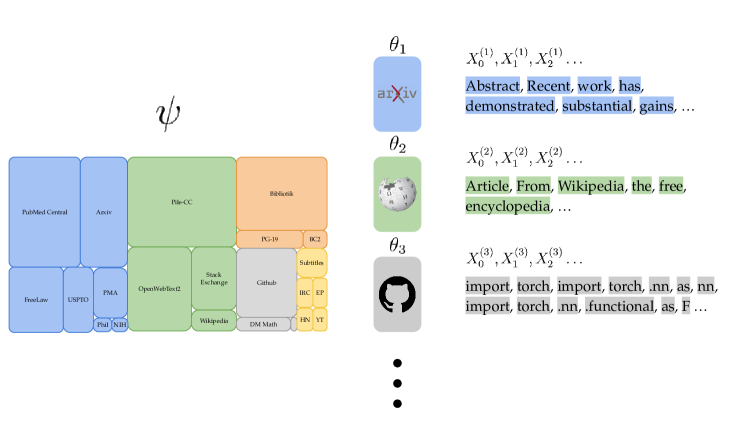
Figure 7: The above diagram depicts the pre-training of large language models as a meta-learning problem. The meta-parameters $\psi$ specify a distribution over document types (tasks). Each document type (task) $\theta_{m}$ specifies an autoregressive random process. Each document $(X^{(m)}_{0},X^{(m)}_{1},X^{(m)}_{2},\ldots)$, is represented by a sequence of tokens which is distributed according to the random process designated by the document type.

8.1 Data Generating Process

In meta-learning assume a further underlying structure in the data that we observe. Concretely, let the random process $(X_{t}^{(m)}:m,t\in\mathbb{Z}_{++})$ denote observations. For any fixed $m$, $(X_{0}^{(m)},X_{1}^{(m)},\ldots)$ represents the data associated with a particular task indexed by $m$. In meta-learning, we assume that there exists a shared structure across the tasks. Learning the structure will often accelerate learning on subsequent tasks. We assume that the sequence $(X_{0:\infty}^{(1)},X_{0:\infty}^{(2)},\ldots)$ is exchangeable i.e. any finite permutation of the sequence does not alter the joint distribution. De Finetti’s theorem then states that there exists a latent random variable, which we will denote by $\psi$ such that conditioned on $\psi$, the above sequence is iid. Note that this iid assumption does not pertain to the observations within a given task, but rather to the entire collections $X_{0:\infty}^{(m)}$ across tasks.

This latent variable $\psi$, which we refer to as the meta-parameters, represents the aforementioned information which is shared across tasks. However, typically in meta-learning, for any particular task, there exists information beyond $\psi$ which must be learned to produce accurate predictions. As a result, we let $(\theta_{1},\theta_{2},\ldots)$ be a sequence which is also iid when conditioned on $\psi$ and we assume that for all $m$, $X_{0:\infty}^{(m)}\perp\psi|\theta_{m}$. For each task $m$, $\theta_{m}$ may subsume the information contained in $\psi$ and contains all other relevant information which can be learned from the intra-task observations.

We again outline that, we do not make the assumption that the intra-task observations are iid when conditioned on $\theta_{m}$. This allows us to characterize more realistic data generating processes such as natural language for which the “tasks” may represent document types and the “observations” the sequence of tokens which comprise of a document of said type (Figure 7).

8.2 Meta-Learning Error

We define notions of error for meta-learning which directly parallel the definitions of section 3.3. For purposes of analysis, we consider learning under a setting for which there exist $M$ tasks and $T$ observations per task. A learning algorithm produces for each $(m,t)\in[M]\times[T]$, a predictive distribution $P_{m,t}$ of $X_{t+1}^{(m)}$ after observing the concatenated history which we denote by

$$H_{m,t}=\left(X^{(1)}_{0:T},X^{(2)}_{0:T},\ldots,X^{(m-1)}_{0:T},X^{(m)}_{0:t}\right).$$

$H_{m,t}$ consists of all observations from tasks $1,\ldots,m-1$ and up to the $t$-th observation of task $m$. We express our meta-learning algorithm in terms of a function $\pi$ for which $P_{m,t}=\pi(H_{m,t})$. For all $M,T\in\mathbb{Z}_{++}$, we measure the error realized by our predictions $P_{m,t}$ in terms of the average cumulative expected log-loss:

$$\mathbb{L}_{M,T,\pi}\ =\ \frac{1}{MT}\sum_{m=1}^{M}\sum_{t=0}^{T-1}\mathbb{E}_{\pi}\left[-\ln P_{m,t}\left(X_{t+1}^{(m)}\right)\right].$$

Since this error is not baselined at $0$, we elect to study the following estimation error:

$$\mathcal{L}_{M,T,\pi}\ =\ \mathbb{L}_{M,T,\pi}-\frac{\mathbb{H}\left(H_{M,T}|\psi,\theta_{1:M}\right)}{MT}.$$

Note that while we introduce this new notation to facilitate exposition of meta-learning, the above notions of error are subsumed by those established in section 3.3.

8.3 Achievable Error

We are again interested in characterizing the limits of performance via machine learning. As a result, it is prudent to answer: For all $(M,T)$, what $\pi$ minimizes $\mathcal{L}_{M,T,\pi}$? As one would expect, the optimal algorithm assigns for all $(m,t)$, $P_{m,t}=\mathbb{P}(X_{t+1}\in\cdot|H_{m,t})$. We will denote this Bayesian posterior which we will denote as $\hat{P}_{m,t}$.

Lemma 45.

(Bayesian posterior is optimal) For all $m,t\in\mathbb{Z}_{+}$,

$$\mathbb{E}\left[-\ln\hat{P}_{m,t}\left(X_{t+1}^{(m)}\right)\right]\ =\ \min_{\pi}\ \mathbb{E}_{\pi}\left[-\ln P_{m,t}\left(X_{t+1}^{(m)}\right)\right].$$

Proof.

$$\mathbb{E}\left[-\ln P_{m,t}\left(X^{(m)}_{t+1}\right)|H_{m,t}\right] \overset{a.s.}{=}\mathbb{E}\left[-\ln\hat{P}_{m,t}\left(X^{(m)}_{t+1}\right)+\ln\frac{\hat{P}_{m,t}\left(X^{(m)}_{t+1}\right)}{P_{m,t}(X^{(m)}_{t+1})}\bigg{|}H_{m,t}\right]$$

$$\overset{a.s.}{=}\mathbb{E}\left[-\ln\hat{P}_{m,t}(X^{(m)}_{t+1})|H_{m,t}\right]+{\mathbf{d}}_{\rm KL}\left(\hat{P}_{m,t}\|P_{m,t}\right).$$

The result follows from the fact that KL-divergence is non-negative and the tower property. ∎

Going forward, we will restrict our attention to the optimal achievable estimation error which we denote by:

$$\mathcal{L}_{M,T}\ =\ \frac{1}{MT}\sum_{t=0}^{T-1}\sum_{m=1}^{M}\ \mathbb{E}\left[-\ln\hat{P}_{m,t}\left(X^{(m)}_{t+1}\right)\right]-\frac{\mathbb{H}(H_{M,T}|\psi,\theta_{1},\ldots,\theta_{M})}{MT}.$$

The process of learning should result in $\mathcal{L}_{M,T}$ vanishing to $0$ as $MT$ increases to $\infty$. We are interested in characterizing the rate at which the estimation error decays to $0$. In previous sections, we established that even if the observations are not iid, we can observe error which decays linearly in the number of observations. In the following section, we will establish general results which bound the estimation error of meta-learning and facilitate the analysis of concrete problem instances.

8.4 General Theoretical Results

We begin with a general result which expresses the estimation error of meta-learning in terms of two very intuitive quantities:

Theorem 46.

(estimation error) For all $M,T\in\mathbb{Z}_{+}$,

$$\mathcal{L}_{M,T} \ =\ \underbrace{\frac{\mathbb{I}(H_{M,T};\psi)}{MT}}_{\begin{subarray}{c}\text{meta}\\ \text{estimation}\\ \text{error}\end{subarray}}\ +\ \sum_{m=1}^{M}\underbrace{\frac{\mathbb{I}(X^{(m)}_{0:T};\theta_{m}|\psi)}{MT}}_{\begin{subarray}{c}\text{intra-task}\\ \text{estimation}\\ \text{error}\end{subarray}}.$$

Proof.

$$\mathcal{L}_{M,T} =\frac{1}{MT}\sum_{m=1}^{M}\sum_{t=0}^{T-1}\ \mathbb{E}\left[-\ln\hat{P}_{m,t}(X^{(m)}_{t+1})\right]-\frac{\mathbb{H}(H_{M,T}|\psi,\theta_{1},\ldots,\theta_{M})}{MT}$$

$$=\frac{1}{MT}\sum_{m=1}^{M}\sum_{t=0}^{T-1}\ \mathbb{I}(X_{t+1}^{(m)};\psi,\theta_{m}|H_{m,t})$$

$$\overset{(a)}{=}\frac{1}{MT}\sum_{m=1}^{M}\mathbb{I}(X^{(m)}_{0:T};\psi,\theta_{m}|H_{m-1,T})$$

$$\overset{(b)}{=}\frac{1}{MT}\sum_{m=1}^{M}\mathbb{I}(X^{(m)}_{0:T};\psi|H_{m-1,T})+\frac{1}{MT}\sum_{m=1}^{M}\mathbb{I}(X^{(m)}_{0:T};\theta_{m}|\psi,H_{m-1,T})$$

$$\overset{(c)}{=}\frac{1}{MT}\sum_{m=1}^{M}\mathbb{I}(X^{(m)}_{0:T};\psi|H_{m-1,T})+\frac{1}{MT}\sum_{m=1}^{M}\mathbb{I}(X^{(m)}_{0:T};\theta_{m}|\psi)$$

$$\overset{(d)}{=}\frac{\mathbb{I}(H_{M,T};\psi)}{MT}+\sum_{m=1}^{M}\frac{\mathbb{I}(X^{(m)}_{0:T};\theta_{m}|\psi)}{MT},$$

where $(a),(b)$, and $(d)$ follow from the chain rule of mutual information, and $(c)$ follows from the meta-learning conditional independence assumptions. ∎

The meta-estimation error term refers to the error which is attributed to learning about the meta-parameters $\psi$. Since all of the observations contain information about $\psi$, it is intuitive that the numerator would include the mutual information between the full history $H_{M,T}$ and the meta-parameters $\psi$. Likewise, it is also to be expected that the error decays linearly in the product $MT$ since each observation contributes information about $\psi$. The second term consists of the error which is incurred from learning about the task specific parameters $\theta_{1},\ldots,\theta_{M}$ conditioned on $\psi$. Note that due to the conditional iid assumptions, this term simplifies to $\mathbb{I}(X_{0:T}^{(m)};\theta_{m}|\psi)/T$. Notably, this term decays linearly in $T$ but not $M$ since the data from other tasks is independent of $\theta^{(m)}$ when conditioned on $\psi$. Intuitively, this error captures the remaining information to be extracted for a particular task beyond what is present in the meta-parameters.

While this result is useful for conceptual understanding, we require further tools to streamline theoretical analysis. We again leverage rate-distortion theory to establish suitable upper and lower bounds for the estimation error of meta-learning. Concretely, we define two rate-distortion functions. The first characterizes the meta-parameters:

$$\mathbb{H}_{\epsilon,M,T}(\psi)\ =\ \inf_{\tilde{\psi}\in\tilde{\Psi}_{\epsilon,M,T}}\ \mathbb{I}(\psi;\tilde{\psi}),$$

where

$$\Psi_{\epsilon,M,T}\ =\ \left\{\tilde{\psi}:\tilde{\psi}\perp H_{M,T};\quad\frac{\mathbb{I}(H_{M,T};\psi|\tilde{\psi})}{MT}\leq\epsilon\right\}.$$

The second characterizes the intra-task parameters conditioned on $\psi$:

$$\mathbb{H}_{\epsilon,T}(\theta_{m}|\psi)\ =\ \inf_{\tilde{\theta}_{m}\in\tilde{\Theta}_{\epsilon,T}}\ \mathbb{I}(\theta_{m};\tilde{\theta}_{m}|\psi),$$

where

$$\tilde{\Theta}_{\epsilon,T}\ =\ \left\{\tilde{\theta}:\tilde{\theta}\perp H_{M,T}\Big{|}\theta_{m};\quad\frac{\mathbb{I}(X^{(m)}_{0:T};\theta_{m}|\tilde{\theta},\psi)}{T}\leq\epsilon\right\}.$$

With these definitions in place, we establish upper and lower bounds on the estimation error in terms of the above rate-distortion functions.

Theorem 47.

(rate-distortion estimation error bound) For all $M,T\in\mathbb{Z}_{+}$, and $m\in\{1,\ldots,M\}$,

$$\mathcal{L}_{M,T} \ \leq\ \inf_{\epsilon\geq 0}\ \frac{\mathbb{H}_{\epsilon,M,T}(\psi)}{MT}+\epsilon\quad+\quad\inf_{\epsilon^{\prime}\geq 0}\ \frac{\mathbb{H}_{\epsilon^{\prime},T}(\theta_{m}|\psi)}{T}+\epsilon^{\prime},$$

and

$$\mathcal{L}_{M,T} \ \geq\ \sup_{\epsilon\geq 0}\min\left\{\frac{\mathbb{H}_{\epsilon,M,T}(\psi)}{MT},\epsilon\right\}\quad+\quad\sup_{\epsilon^{\prime}\geq 0}\min\left\{\frac{\mathbb{H}_{\epsilon^{\prime},T}(\theta_{m}|\psi)}{T},\epsilon^{\prime}\right\}.$$

Proof.

We begin by showing the upper bound:

$$\mathcal{L}_{M,T} =\frac{\mathbb{I}(H_{M,T};\psi)}{MT}+\frac{\mathbb{I}(X^{(m)}_{0:T};\theta_{m}|\psi)}{T}$$

$$=\frac{\mathbb{I}(H_{M,T};\psi,\tilde{\psi})}{MT}+\frac{\mathbb{I}(X^{(m)}_{0:T};\theta_{m},\tilde{\theta}_{m}|\psi)}{T}$$

$$=\frac{\mathbb{I}(H_{M,T};\tilde{\psi})}{MT}+\frac{\mathbb{I}(H_{M,T};\psi|\tilde{\psi})}{MT}+\frac{\mathbb{I}(X^{(m)}_{0:T};\theta_{m},\tilde{\theta}_{m}|\psi)}{T}$$

$$\overset{(a)}{\leq}\frac{\mathbb{I}(\psi;\tilde{\psi})}{MT}+\frac{\mathbb{I}(H_{M,T};\psi|\tilde{\psi})}{MT}+\frac{\mathbb{I}(X^{(m)}_{0:T};\theta_{m},\tilde{\theta}_{m}|\psi)}{T}$$

$$=\frac{\mathbb{I}(\psi;\tilde{\psi})}{MT}+\frac{\mathbb{I}(H_{M,T};\psi|\tilde{\psi})}{MT}+\frac{\mathbb{I}(X^{(m)}_{0:T};\tilde{\theta}_{m}|\psi)}{T}+\frac{\mathbb{I}(X^{(m)}_{0:T};\theta_{m}|\tilde{\theta}_{m},\psi)}{T}$$

$$\overset{(b)}{\leq}\frac{\mathbb{I}(\psi;\tilde{\psi})}{MT}+\frac{\mathbb{I}(H_{M,T};\psi|\tilde{\psi})}{MT}+\frac{\mathbb{I}(\theta_{m};\tilde{\theta}_{m}|\psi)}{T}+\frac{\mathbb{I}(X^{(m)}_{0:T};\theta_{m}|\tilde{\theta}_{m},\psi)}{T}$$

$$\overset{(c)}{\leq}\frac{\mathbb{H}_{\epsilon,M,T}(\psi)}{MT}+\epsilon+\frac{\mathbb{H}_{\epsilon^{\prime},M,T}(\tilde{\theta}_{m}|\psi)}{T}+\epsilon^{\prime},$$

where $(a)$ and $(b)$ follow from the data processing inequality and $(c)$ follows from the definition of the rate-distortion functions. The upper bound follows from the fact that inequality $(c)$ holds for all $\epsilon\geq 0$.

We now prove the lower bound. Suppose that $\mathbb{I}(H_{M,T};\psi)<\mathbb{H}_{\epsilon,M,T}(\psi)$ Let $\tilde{\psi}=\tilde{H}_{M,T}\notin\tilde{\Psi}_{\epsilon,M,T}$ where $\tilde{H}_{M,T}$ is another history sampled in the same manner as $H_{M,T}$.

$$\mathbb{I}(H_{M,T};\psi) =\sum_{m=1}^{M}\sum_{t=0}^{T-1}\mathbb{I}(X^{(m)}_{t+1};\psi|H_{m,t})$$

$$\overset{(a)}{\geq}\sum_{m=1}^{M}\sum_{t=0}^{T-1}\mathbb{I}(X^{(m)}_{t+1};\psi|\tilde{H}_{M,T},H_{m,t})$$

$$=\sum_{m=1}^{M}\sum_{t=0}^{T-1}\mathbb{I}(X^{(m)}_{t+1};\psi|\tilde{\psi},X^{(m)}_{1},\ldots,X^{(m)}_{t})$$

$$\overset{(b)}{\geq}\epsilon MT,$$

where $(a)$ follows from the fact that conditioning reduces entropy and that $X^{(m)}_{t+1}\perp\tilde{H}_{M,T}|(\psi,H_{m,t})$ and $(b)$ follows from the fact that $\tilde{\psi}\notin\tilde{\Psi}_{\epsilon,M,T}$. Therefore, for all $\epsilon\geq 0$, $\mathbb{I}(H_{M,T};\psi)\geq\min\{H_{\epsilon,M,T}(\psi),\epsilon MT\}$.

Suppose that $\mathbb{I}(H_{T}^{(m)};\theta_{m}|\psi)<\mathbb{H}_{\epsilon,T}(\theta_{m}|\psi)$. Let $\tilde{\theta}_{m}=\tilde{D}_{m}\notin\tilde{\Theta}_{\epsilon,T}$ where $\tilde{D}_{m}$ is another history sampled in the same manner as $X^{(m)}_{0:T}$.

$$\mathbb{I}(X^{(m)}_{0:T};\theta_{m}|\psi) =\sum_{t=0}^{T-1}\mathbb{I}(X^{(m)}_{t+1};\theta_{m}|X^{(m)}_{1},\ldots,X^{(m)}_{t},\psi)$$

$$\overset{(a)}{\geq}\sum_{t=0}^{T-1}\mathbb{I}(X^{(m)}_{t+1};\theta_{m}|\tilde{D}_{m},X^{(m)}_{1},\ldots,X^{(m)}_{t},\psi)$$

$$=\sum_{t=0}^{T-1}\mathbb{I}(X^{(m)}_{t+1};\theta_{m}|\tilde{\theta}_{m},H_{m,t},\psi)$$

$$\overset{(b)}{\geq}\epsilon T,$$

where $(a)$ follows from the fact that conditioning reduces entropy and that $X^{(m)}_{t+1}\perp\tilde{D}_{m}|(\psi,X^{(m)}_{1},\ldots,X^{(m)}_{t})$ and $(b)$ follows from the fact that $\tilde{\theta}_{m}\notin\tilde{\Theta}_{\epsilon,T}$. Therefore, for all $\epsilon\geq 0$, $\mathbb{I}(X^{(m)}_{0:T};\theta_{m}|\psi)\geq\min\{H_{\epsilon,M,T}(\theta_{m}),\epsilon T\}$. The lower bound follows as a result. ∎

Theorem 47 establishes an intimate connection between the estimation error of meta learning and the aforementioned rate-distortion functions via upper and lower bounds. This result will allow us to streamline the analysis of learning under various meta-learning problems. In the subsequent sections, we will study two such instances. The first is a simple linear representation learning setting which is provided as exposition to acclimate the reader to the styles of analysis required for meta-learning. The second setting involves a mixture of transformers which resembles and provides insights about pre-training and in-context learning in LLMs.

8.5 Linear Representation Learning

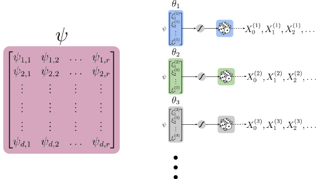
Figure 8: The above diagram depicts the linear representation learning problem. The matrix $\psi\in\Re^{d\times r}$ represents the information which is shared across the tasks. The intra-task information $\theta_{m}$ is the product $\psi\xi^{(m)}$, where $\xi^{(m)}\in\Re^{r}$. The resulting vector $\theta_{m}$ is passed through a softmax to produce a categorical distribution over $d$ classes. Each corresponding sequence $X^{(m)}_{0},X^{(m)}_{1},X^{(m)}_{2},\ldots$ is produce via iid sampling of the aforementioned categorical distribution.

8.5.1 Data Generating Process

We introduce a simple linear representation learning problem as a concrete example of meta-learning to demonstrate our method of analysis. In this example, the intra-task observations are iid, but we begin with such an example for simplicity and to demonstrate this as a special case of general meta-learning under our framework.

For all $d,r\in\mathbb{Z}_{++}$, we let $\psi:\Omega\mapsto\Re^{d\times r}$ be distributed uniformly over the set of $d\times r$ matrices with orthonormal columns. We assume that $d\gg r$. For all $m$, let $\xi^{(m)}:\Omega\mapsto\Re^{r}$ be distributed iid $\mathcal{N}(0,I_{r}/r)$. We let $\theta_{m}=\psi\xi^{(m)}$. As for the observable data, for each $(m,t)$, let $X_{t+1}^{(m)}$ be drawn as according to the following probability law:

$$X^{(m)}_{t+1}=\begin{cases}1&\text{w.p. }\sigma(\theta_{m})_{1}\\ 2&\text{w.p. }\sigma(\theta_{m})_{2}\\ \ldots&\\ d&\text{w.p. }\sigma(\theta_{m})_{d}\\ \end{cases},$$

where $\sigma(\theta_{m})_{j}=e^{\theta_{m,j}}/\sum_{k=1}^{d}e^{\theta_{m,k}}$. For each task $m$, the algorithm is tasked with estimating a vector $\theta_{m}$ from sampled observations $(X_{1}^{(m)},X_{2}^{(m)},\ldots)$. By reasoning about data from previous tasks, the algorithm can estimate $\psi$, which reduces the burden of estimating $\theta_{m}$ to just estimating $\xi^{(m)}$ for each task. This is significant given the assumption that $d\gg r$.

8.5.2 Theoretical Building Blocks

We begin by establishing several lemmas which streamline our analysis. We begin with the following upper bound on the meta-estimation error term:

Lemma 48.

(meta rate-distortion upper bound) For all $d,r,M,T\in\mathbb{Z}_{++}$, if for all $(m,t)\in[M]\times[T]$, $X_{t}^{(m)}$ is generated according to the linear representation learning process, then

$$\mathbb{H}_{M,T,\epsilon}(\psi)\ \leq\ \frac{dr}{2MT}\ln\left(1+\frac{d}{r\left(e^{\frac{2\epsilon T}{r}}-1\right)}\right).$$

Proof.

Let $\tilde{\psi}=\psi+Z$ where $Z\in\Re^{d\times r}$ is independent of $\psi$ and consists of elements which are distributed iid $\mathcal{N}(0,\epsilon^{\prime})$ where $\epsilon^{\prime}=(e^{\frac{2\epsilon T}{r}}-1)/d$ We begin by upper bounding the rate.

$$\frac{\mathbb{I}(\psi;\tilde{\psi})}{MT} =\frac{\mathbf{h}(\tilde{\psi})-\mathbf{h}(\tilde{\psi}|\psi)}{MT}$$

$$\overset{(a)}{\leq}\frac{\frac{dr}{2}\ln\left(2\pi e\left(\epsilon^{\prime}+\frac{1}{r}\right)\right)-\frac{dr}{2}\ln\left(2\pi e\epsilon^{\prime}\right)}{MT}$$

$$=\frac{dr\ln\left(1+\frac{1}{r\epsilon^{\prime}}\right)}{2MT}$$

$$=\frac{dr}{2MT}\ln\left(1+\frac{d}{r\left(e^{\frac{2\epsilon T}{r}}-1\right)}\right),$$

where $(a)$ follows from the maximum differential entropy of a random variable of fixed variance being upper bounded by a Gaussian random variable.

We now upper bound the distortion.

$$\frac{\mathbb{I}(H_{M,T};\psi|\tilde{\psi})}{MT} =\frac{\mathbb{H}(H_{M,T}|\tilde{\psi})-\mathbb{H}(H_{M,T}|\psi)}{MT}$$

$$=\frac{\sum_{m=1}^{M}\mathbb{H}(X_{0:T}^{(m)}|\tilde{\psi},H_{m-1,T})-\mathbb{H}(X_{0:T}^{(m)}|\psi,H_{m-1,T})}{MT}$$

$$\leq\frac{\mathbb{H}(X_{0:T}^{(1)}|\tilde{\psi})-\mathbb{H}(X_{0:T}^{(1)}|\psi)}{T}$$

$$=\frac{\mathbb{I}(X_{0:T}^{(1)};\psi|\tilde{\psi})}{T}$$

$$\leq\frac{\mathbb{I}(\theta_{1};\psi|\tilde{\psi})}{T}$$

$$=\frac{\mathbb{E}\left[{\mathbf{d}}_{\rm KL}(\mathbb{P}(\theta_{1}\in\cdot|\psi)\|\mathbb{P}(\theta_{1}\in\cdot|\tilde{\psi}))\right]}{n}$$

$$\overset{(a)}{\leq}\frac{\mathbb{E}\left[{\mathbf{d}}_{\rm KL}(\mathbb{P}(\theta_{1}\in\cdot|\psi)\|\mathbb{P}(\theta_{\in}\cdot|\psi\leftarrow\tilde{\psi}))\right]}{T}$$

$$\leq\frac{\mathbb{E}\left[{\mathbf{d}}_{\rm KL}(\lim_{\delta\to 0}\mathbb{P}(\theta_{\delta}\in\cdot|\psi)\|\lim_{\delta\to 0}\mathbb{P}(\theta_{\delta}|\psi\leftarrow\tilde{\psi}))\right]}{T}$$

$$\overset{(b)}{=}\frac{1}{T}\mathbb{E}\left[\lim_{\delta\to 0}\frac{1}{2}\ln\left(\frac{\left|\delta I_{d}+\frac{\tilde{\psi}\tilde{\psi}^{\top}}{r}\right|}{\left|\delta I_{d}+\frac{\psi\psi^{\top}}{r}\right|}\right)-d+{\rm Tr}\left(\left(\delta I_{d}+\frac{\tilde{\psi}\tilde{\psi}^{\top}}{r}\right)^{-1}\left(\delta I_{d}+\frac{\psi\psi^{\top}}{r}\right)\right)\right]$$

$$\overset{(c)}{\leq}\frac{1}{T}\mathbb{E}\left[\lim_{\delta\to 0}\frac{1}{2}\ln\left(\frac{\left|\delta I_{d}+\frac{\tilde{\pi}\tilde{\psi}^{\top}}{r}\right|}{\left|\delta I_{d}+\frac{\psi\psi^{\top}}{r}\right|}\right)\right]$$

$$\overset{(d)}{=}\frac{1}{T}\mathbb{E}\left[\lim_{\delta\to 0}\frac{1}{2}\ln\left(\frac{\left|\delta I_{d}\right|\cdot\left|I_{r}+\frac{\tilde{\psi}^{\top}\tilde{\psi}}{r\delta}\right|}{\left|\delta I_{d}\right|\cdot\left|I_{r}+\frac{\psi^{\top}\psi}{r\delta}\right|}\right)\right]$$

$$=\frac{1}{T}\mathbb{E}\left[\lim_{\delta\to 0}\frac{1}{2}\ln\left(\frac{\left|I_{r}+\frac{\tilde{\psi}^{\top}\tilde{\psi}}{r\delta}\right|}{\left|I_{r}+\frac{I_{r}}{r\delta}\right|}\right)\right]$$

$$\overset{(e)}{\leq}\lim_{\delta\to 0}\frac{1}{2T}\ln\left(\frac{\left|I_{r}+\frac{\mathbb{E}\left[\tilde{\psi}^{\top}\tilde{\psi}\right]}{r\delta}\right|}{\left|I_{r}+\frac{I_{r}}{r\delta}\right|}\right)$$

$$=\lim_{\delta\to 0}\frac{1}{2T}\ln\left(\frac{\left|I_{r}+\frac{\mathbb{E}\left[I_{r}+d\epsilon^{\prime}I_{r}\right]}{r\delta}\right|}{\left|I_{r}+\frac{I_{r}}{r\delta}\right|}\right)$$

$$=\lim_{\delta\to 0}\frac{r}{2T}\ln\left(\frac{1+\frac{1+d\epsilon^{\prime}}{r\delta}}{1+\frac{1}{r\delta}}\right)$$

$$=\frac{r}{2T}\ln\left(1+d\epsilon\right)$$

$$=\epsilon,$$

where $(a)$, $(b)$ follows from continuity of the KL-divergence between two multivariate normal distributions w.r.t the covariance matrix, $(c)$ follows from the fact that the trace term is upper bounded by $d$, $(d)$ follows from the matrix determinant lemma, $\epsilon=\frac{1}{m}$, and $(e)$ follows from Jensen’s inequality. The result follows. ∎

Recall that for meta-learning, the total estimation error is upper bounded by the sum of the meta rate-distortion function and the intra-task rate-distortion function. The following result establishes an upper bound on the intra-task rate-distortion function.

Lemma 49.

(intra-task rate-distortion upper bound) For all $r,T\in\mathbb{Z}_{++}$,

$$\mathbb{H}_{T,\epsilon}(\theta_{m}|\psi)\ \leq\ \frac{r}{2}\ln\left(1+\frac{1}{\epsilon}\right).$$

Proof.

Let $\tilde{\xi}=\xi^{(m)}+Z$ where $Z\perp\xi^{(m)}$ and $Z\sim\mathcal{N}(0,\epsilon I_{r}/r)$. Let $\tilde{\theta}=\psi\tilde{\xi}$. We begin by upper bounding the rate.

$$\mathbb{I}(\theta_{m};\tilde{\theta}|\psi) \leq\mathbb{I}(\xi;\tilde{\xi}|\psi)$$

$$=\mathbf{h}(\tilde{\xi}|\psi)-\mathbf{h}(\tilde{\xi}|\psi,\xi)$$

$$=\mathbf{h}(\tilde{\xi})-\mathbf{h}(\tilde{\xi}|\xi)$$

$$=\mathbf{h}(\tilde{\xi})-\mathbf{h}(Z)$$

$$=\frac{r}{2}\ln\left(2\pi e(\frac{\epsilon}{r}+\frac{1}{r})\right)-\frac{r}{2}\ln\left(\frac{2\pi e\epsilon}{r}\right)$$

$$=\frac{r}{2}\ln\left(1+\frac{1}{\epsilon}\right).$$

We now upper bound the distortion:

$$\frac{\mathbb{I}(X^{(m)}_{0:T};\theta_{m}|\tilde{\theta},\psi)}{T} \leq\frac{\mathbb{I}(X^{(m)}_{0:T};\theta_{m}|\tilde{\theta},\psi)}{T}$$

$$\leq\mathbb{I}(X_{1}^{(m)};\theta_{m}|\tilde{\theta})$$

$$=\mathbb{E}\left[{\mathbf{d}}_{\rm KL}\left(\mathbb{P}\left(X^{(m)}_{1}\in\cdot|\theta_{m}\right)\|\mathbb{P}\left(X^{(m)}_{1}\in\cdot|\tilde{\theta}\right)\right)\right]$$

$$\overset{(a)}{\leq}\mathbb{E}\left[{\mathbf{d}}_{\rm KL}\left(\mathbb{P}\left(X^{(m)}_{1}\in\cdot|\theta_{m}\right)\|\mathbb{P}\left(X^{(m)}_{1}\in\cdot|\theta_{m}\leftarrow\tilde{\theta}\right)\right)\right]$$

$$\overset{(b}{\leq}\mathbb{E}\left[\|\tilde{\theta}-\theta_{m}\|^{2}_{2}\right]$$

$$=\mathbb{E}\left[\left(\xi^{(m)}-\tilde{\xi}\right)^{\top}\psi^{\top}\psi\left(\xi^{(m)}-\tilde{\xi}\right)\right]$$

$$=\mathbb{E}\left[\left(\xi^{(m)}-\tilde{\xi}\right)^{\top}\left(\xi^{(m)}-\tilde{\xi}\right)\right]$$

$$=\mathbb{E}\left[Z^{\top}Z\right]$$

$$=\epsilon$$

where $(a)$ follows from Lemma 1, and $(b)$ follows from Lemma 23. ∎

With these two results in place, we present the main result which upper bounds the estimation error of linear representation learning.

8.5.3 Main Result

With the rate-distortion upper bounds established from the previous section, we present the following reslt which upper bounds the estimation error of linear representation learning.

Theorem 50.

(linear representation learning estimation error bound) For all $d,r,M,T\in\mathbb{Z}_{++}$, if for all $(m,t)$, $X^{(m)}_{t}$ is generated according to the linear representation learning process, then

$$\mathcal{L}_{M,T} \ \leq\ \frac{dr\ln\left(e\left(1+\frac{M}{r}\right)\right)}{2MT}+\frac{r\ln\left(e\left(1+\frac{2T}{r}\right)\right)}{2T}.$$

Proof.

$$\mathcal{L}_{M,T} \overset{(a)}{\leq}\inf_{\epsilon\geq 0}\ \frac{\mathbb{H}_{M,T\epsilon}(\psi)}{MT}+\epsilon+\inf_{\epsilon^{\prime}\geq 0}\ \frac{\mathbb{H}_{T,\epsilon^{\prime}}(\theta_{m}|\psi)}{T}+\epsilon^{\prime}$$

$$\overset{(b)}{\leq}\inf_{\epsilon\geq 0}\ \frac{dr}{2MT}\ln\left(1+\frac{d}{r\left(e^{\frac{2\epsilon T}{r}}-1\right)}\right)+\epsilon+\inf_{\epsilon^{\prime}\geq 0}\frac{r}{2n}\ln\left(1+\frac{1}{r\epsilon^{\prime}}\right)+\epsilon^{\prime}$$

$$\overset{(c)}{\leq}\frac{dr}{2MT}\ln\left(1+\frac{d}{r\left(e^{\frac{d\epsilon}{M}}-1\right)}\right)+\frac{dr}{2MT}+\frac{r\ln(1+\frac{2T}{r})}{2T}+\frac{r}{2T}$$

$$\leq\frac{dr\ln\left(1+\frac{M}{r}\right)}{2MT}+\frac{dr}{2MT}+\frac{r\ln(1+\frac{2T}{r})}{2T}+\frac{r}{2T}$$

$$=\frac{dr\ln\left(e\left(1+\frac{M}{r}\right)\right)}{2MT}+\frac{r\ln\left(e\left(1+\frac{2T}{r}\right)\right)}{2T},$$

where $(a)$ follows from Theorem 46, $(b)$ follows directly from Lemmas 48 and 49, and $(c)$ follows from setting $\epsilon=\frac{dr}{2MT}$ and $\epsilon^{\prime}=\frac{r}{2T}$. ∎

The first term describes the error which is incurred in the process of estimating the meta-parameters $\psi$. Notably, this term is linear in $dr$, the parameter count of $\psi$ and decays linearly in $MT$, the total number of observations. This is both intuitive and desirable since each observation ought to provide information about $\psi$. Meanwhile, the second term describes the error which is incurred in the process of estimating the intra-task parameters $\theta_{m}$ conditioned on $\psi$. In our problem instance, $\theta=\psi\xi$ for $\xi\in\Re^{r}$, so the remaining uncertainty in $\theta$ when conditioning on $\psi$ is simply $\xi$. Therefore, the intra-task error is linear in $r$, the parameter count of $\xi$ and decays linearly in $T$, the number of observations pertinent to task $m$.

In the following section, we will characterize the learning performance under a much more complex process which resembles pre-training and in-context learning in LLMs.

8.6 In-Context Learning

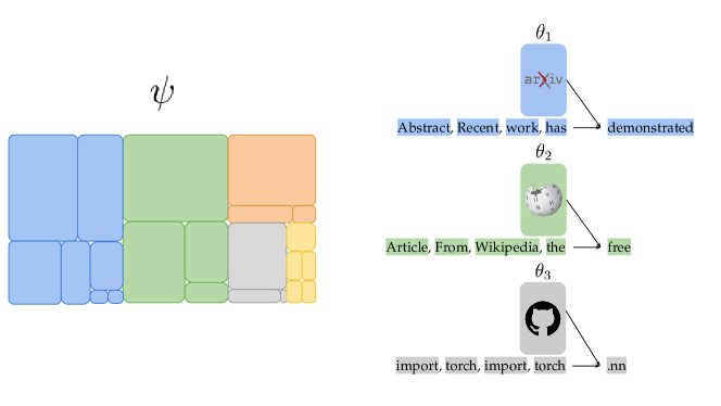
Figure 9: The above diagram depicts the in-context learning problem. $\psi$ designates a mixture of many transformer models, each which is responsible for producing documents of a particular type. Each document is generated by sampling a transformer model $\theta_{m}$ from the mixture $\psi$, and generating a sequence $(X_{0}^{(m)},X_{1}^{(m)},X_{2}^{(m)},\ldots)$ autoregressively.

8.6.1 Data Generating Process

In the ICL process, for all documents $m$, we let its tokens $(X^{(m)}_{1},X^{(m)}_{2},\ldots)$ be a sequence in $\{1,\ldots,d\}$, where $d$ denotes the size of the vocabulary. Each of the $d$ outcomes is associated with a known embedding vector which we denote as $\Phi_{j}$ for $j\in\{1,\ldots,d\}$. We assume that for all $j$, $\|\Phi_{j}\|_{2}=1$. For brevity of notation, we let $\phi_{t}^{(m)}=\Phi_{X^{(m)}_{t}}$ i.e. the embedding associated with token $X^{(m)}_{t}$.

Each document is generated by a transformer model which is sampled iid from a mixture. We assume that sampling is performed according to a categorical distribution parameterized by $\alpha$ with prior distribution $\mathbb{P}(\alpha\in\cdot)=\text{Dirichlet}(N,[R/N,\ldots,R/N])$ for a scale parameter $R\ll N$. Realizations of this prior distributions are hence probability mass function on the classes $\{1,2,\ldots,N\}$. If we sample $M$ times from this pmf, we recover a Dirichlet-multinomial for which the expected number of unique classes grows linearly in $R$ and only logarithmically in $M$. This may be representative of the documents which comprise of an internet corpus. The vast majority will belong to one of several prominent classes such as academic literature, articles, question-answer, etc. However, there may be several documents which are rather spurious in relation to the remainder of the corpus. Therefore, we permit the number of document types $N$ to potentially be exponentially large, but we assume that the scale parameter $R$ remains modest.

Each of the $N$ elements of the mixture corresponds to a transformer network as outlined in Section 7.3. Let $K$ denote the context lengths of the transformers, $L$ denote their depths, and $r$ their attention dimensions. Let $\psi_{1},\ldots,\psi_{N}$ denote the weights of the transformer mixture elements. As a result, the meta-parameters $\psi=(\alpha,\psi_{1},\ldots,\psi_{N})$ i.e. the mixture sampling weights and the mixture model weights.

For all $t$, the generation of token $X^{(m)}_{t+1}$ will depend on the sampled mixture index $i_{m}\in\{1,\ldots,N\}$, the corresponding transformer weights $\psi_{i_{m}}$ and the previous $K$ tokens $X^{(m)}_{t-K+1},\ldots,X^{(m)}_{t}$. We use $U^{(m)}_{t,\ell}$ to denote the output of layer $\ell$ at time $t$ for document $m$. For all $m,t$, we let $(U^{(m)}_{t,0}=\phi_{t-K+1:t})$ be the embeddings associated with the past $K$ tokens. For $\ell>0$, we let $U^{(m)}_{t,\ell}$ denote the output of layer $\ell$ of the transformer with input $U^{(m)}_{t,0}$. For all $t\leq T,i<L,m\leq M$, let

$$\text{Attn}^{(\ell)}\left(U^{(m)}_{t,\ell-1}\right)={\rm Softmax}\left(\frac{U^{(m)\top}_{t,\ell-1}A^{(m)}_{\ell}U^{(m)}_{t,\ell-1}}{\sqrt{r}}\right)$$

denote the attention matrix of layer $\ell$ for document $m$ where the softmax function is applied elementwise along the columns. The matrix $A^{(m)}_{\ell}\in\Re^{r\times r}$ can be interpreted as the product of the key and query matrices and we assume that the elements of the matrices $A^{(m)}_{\ell}$ are distributed iid $\mathcal{N}(0,1)$.

Subsequently, we let

$$U^{(m)}_{t,\ell}=\text{Clip}\left(V^{(m)}_{\ell}U^{(m)}_{t,\ell-1}\text{Attn}^{(\ell)}\left(U^{(m)}_{t,\ell-1}\right)\right),$$

where Clip ensures that each column of the matrix input has $L_{2}$ norm at most $1$. The matrix $V^{(m)}_{\ell}$ resembles the value matrix and we assume that the elements of $V^{(m)}_{\ell}$ are distributed iid $\mathcal{N}(0,1/d)$.

Finally, the next token is generated via sampling from the softmax of the final layer:

$$X^{(m)}_{t+1}\sim{\rm Softmax}\left(U^{(m)}_{t,L}[-1]\right),$$

where $U^{(m)}_{t,L}[-1]$ denotes the right-most column of $U^{(m)}_{t,L}$. At each layer $\ell$, the parameters consist of the matrices $A^{(m)}_{\ell},V^{(m)}_{\ell}$. As a result, the intra-task parameters consist of $\theta_{m}=(i_{m},\psi_{i_{m}})$ i.e. the mixture index and the weights of the corresponding transformer model.

8.6.2 Theoretical Building Blocks

To obtain the tightest bounds for this problem instance, instead of consider two separate rate-distortion functions as in Theorem 47, we must instead analyze the combined rate-distortion function defined below:

$$\mathbb{H}_{M,T,\epsilon}(\psi,\theta_{1:M})\ =\ \inf_{\tilde{\theta}\in\tilde{\Theta}_{M,T,\epsilon}}\ \mathbb{I}(\psi,\theta_{1:M};\tilde{\theta}),$$

where

$$\tilde{\Theta}_{M,T,\epsilon}\ =\ \left\{\tilde{\theta}:\tilde{\theta}\perp H_{M,T}|\theta_{1:M};\quad\frac{\mathbb{I}(H_{M,T};\psi,\theta_{1:M}|\tilde{\theta})}{MT}\leq\epsilon\right\}.$$

Under this rate-distortion function, we obtain the following bounds on estimation error:

Theorem 51.

(rate-distortion estimation error bound 2) For all $M,T\in\mathbb{Z}_{+}$,

$$\mathcal{L}_{M,T}\ \leq\ \inf_{\epsilon\geq 0}\ \frac{\mathbb{H}_{M,T,\epsilon}(\psi,\theta_{1:M})}{MT}+\epsilon,$$

and

$$\mathcal{L}_{M,T}\ \geq\ \sup_{\epsilon\geq 0}\ \min\left\{\frac{\mathbb{H}_{M,T,\epsilon}(\psi,\theta_{1:M})}{MT},\ \epsilon\right\}.$$

Proof.

We begin by establishing the upper bound.

$$\mathcal{L}_{M,T} =\frac{\mathbb{I}(H_{M,T};\psi,\theta_{1:M})}{MT}$$

$$=\inf_{\tilde{\theta}\in\tilde{\Theta}_{M,T,\epsilon}}\ \frac{\mathbb{I}(H_{M,T};\psi,\theta_{1:M},\tilde{\theta})}{MT}$$

$$=\inf_{\tilde{\theta}\in\tilde{\Theta}_{M,T,\epsilon}}\ \frac{\mathbb{I}(H_{M,T};\tilde{\theta})}{MT}+\frac{\mathbb{I}(H_{M,T};\theta_{1:M}|\tilde{\theta})}{MT}$$

$$\leq\frac{\mathbb{H}_{M,T,\epsilon}(\psi,\theta_{1:M})}{MT}+\epsilon.$$

We now establish the lower bound. Suppose that $\mathbb{I}(H_{M,T};\psi,\theta_{1:M})<\mathbb{H}_{M,T,\epsilon}(\psi,\theta_{1:M})$. Let $\tilde{\theta}=\tilde{H}_{M,T}\notin\tilde{\Theta}_{M,T,\epsilon}$ where $\tilde{H}_{M,T}$ is another independent history sampled in the same manner as $H_{M,T}$.

$$\mathbb{I}(H_{M,T};\psi,\theta_{1:M}) =\mathbb{H}(H_{M,T})-\mathbb{H}(H_{M,T}|\psi,\theta_{1:M})$$

$$\overset{(a)}{=}\mathbb{H}(H_{M,T})-\mathbb{H}(H_{M,T}|\psi,\theta_{1:M},\tilde{\theta})$$

$$\overset{(b)}{\geq}\mathbb{H}(H_{M,T}|\tilde{\theta})-\mathbb{H}(H_{M,T}|\psi,\theta_{1:M},\tilde{\theta})$$

$$=\mathbb{I}(H_{M,T};\psi,\theta_{1:M}|\tilde{\theta})$$

$$\overset{(c)}{\geq}\epsilon MT$$

where $(a)$ follows from conditional independence assumptions, $(b)$ follows from the fact that conditioning reduces entropy, and $c)$ follows from the fact that $\tilde{\theta}\notin\tilde{\Theta}_{M,T,\epsilon}$. Therefore, for all $\epsilon\geq 0,\ \mathbb{I}(H_{M,T};\psi,\theta_{1:M})\geq\min\{\mathbb{H}_{M,T,\epsilon}(\psi,\theta_{1:M}),\epsilon MT\}$. The result follows. ∎

With this rate-distortion bound in place, we established that in order to bound the estimation error of ICL, we simply must bound the rate-distortion function. In the following result, we establish an upper bound on the rate-distortion function for the ICL problem.

Lemma 52.

(in-context learning rate-distortion upper bound) For all $d,r,K,L,M,T$, if for all $(m,t)\in[M]\times[T]$, $X^{(m)}_{t}$ is generated by the ICL process, then

$$\mathbb{H}_{M,T,\epsilon}(\psi,\theta_{1:M})\ \leq\ M\ln(N)+R\ln\left(1+\frac{M}{R}\right)\cdot r\cdot\max\{r,d\}L\ln\left(1+\frac{r\cdot\max\{r,d\}KLT(8K(1+16K))^{L}}{\epsilon}\right).$$

Proof.

For the ICL data generating process, we will construct a compression which incrementally builds up elements of the mixture. Concretely, let $\tilde{\theta}=(i_{1},i_{2},\ldots,i_{M},\tilde{\psi})$ where $\psi=\{\tilde{\psi}_{j}:j\in\{i_{1},i_{2},\ldots,i_{M}\}\}$ and $\tilde{\psi}_{j}$ represents a noisy version of $\psi_{j}$. We will use $\mathcal{I}_{M}$ to denote the set of unique indices from $\{i_{1},i_{2},\ldots,i_{M}\}$.

Let $\tilde{\psi}_{j}=(\tilde{V}_{j,\ell},\tilde{A}_{j,\ell}:\ell\in[L])$ where

$$\left(\tilde{V}_{j,\ell},\tilde{A}_{j,\ell}\right)=\left(V_{j,\ell}+Z_{j,\ell},\ A_{j,\ell}+B_{j,\ell}\right)$$

$$(Z_{j,\ell},B_{j,\ell})\perp(V_{j,\ell},A_{j,\ell}),\quad Z_{j,\ell}\overset{iid}{\sim}\begin{cases}\mathcal{N}(0,\epsilon^{\prime}/r^{2})&\text{ if }\ell<L\\ \mathcal{N}(0,\epsilon^{\prime}/(rd)&\text{ if }\ell=L\\ \end{cases};\quad B_{j,\ell}\overset{iid}{\sim}\mathcal{N}(0,\epsilon^{\prime}/r^{2}),$$

and $\epsilon^{\prime}=\frac{\epsilon}{KLT(8K(1+16K))^{L}}$.

We begin by upper bounding the rate.

$$\mathbb{I}(\psi,\theta_{1:M};\tilde{\theta}) =\mathbb{I}(\psi,\theta_{1:M};(i_{1},\ldots,i_{M}),\tilde{\psi})$$

$$=\mathbb{I}(\psi,(i_{1},\ldots,i_{M});(i_{1},\ldots,i_{M}),\tilde{\psi})$$

$$=\mathbb{H}(i_{1},\ldots,i_{M})+\mathbb{I}(\psi;\tilde{\psi}|(i_{1},\ldots,i_{M}))$$

$$\leq M\ln(N)+\mathbb{E}\left[\sum_{i=1}^{N}\mathbbm{1}_{[i\in\mathcal{I}_{M}]}\cdot\mathbb{I}(\psi_{i};\tilde{\psi}_{i})\right]$$

$$\overset{(a)}{\leq}M\ln(N)+R\ln\left(1+\frac{M}{R}\right)\cdot r\cdot\max\{r,d\}L\ln\left(1+\frac{r\cdot\max\{r,d\}KLT(8K(1+16K))^{L}}{\epsilon}\right),$$

where $(a)$ follows from Lemmas 33 and 43.

We now upper bound the distortion:

$$\frac{\mathbb{I}(H_{M,T};\psi,\theta_{1:M}|\tilde{\theta})}{MT} =\frac{\mathbb{I}(H_{M,T};\theta_{1:M}|\tilde{\theta})}{MT}$$

$$=\sum_{m=1}^{M}\frac{\mathbb{I}(X^{(m)}_{0:T};\theta_{1:M}|\tilde{\theta},H_{m-1,T})}{MT}$$

$$\leq\frac{\mathbb{I}(X^{(1)}_{0:T};\theta_{1:M}|\tilde{\theta})}{T}$$

$$=\frac{\mathbb{I}(X^{(1)}_{0:T};\theta_{1}|\tilde{\psi}_{i_{1}})}{T}$$

$$\overset{(a)}{\leq}\epsilon,$$

where $(a)$ follows from Lemma 43. ∎

8.6.3 Main Result

With the rate-distortion results established from the previous section, we establish the following upper bound on the estimation error of in-context learning.

Theorem 53.

(in-context learning estimation error upper bound) For all $d,r,L,K,R,N,M,T\in\mathbb{Z}_{++}$, if for all $(m,t)\in[M]\times[T]$, $X^{(m)}_{t}$ is generated according to the ICL process, then

$$\mathcal{L}_{M,T}\ \leq\ \frac{r\max\{r,d\}RL^{2}\ln\left(1+\frac{M}{R}\right)\ln\left(8Ke(1+16K)\right)}{MT}+\frac{r\max\{r,d\}RL\ln\left(1+\frac{M}{R}\right)\ln\left(\frac{2KMT^{2}}{L}\right)}{MT}+\frac{\ln(N)}{T}.$$

Proof.

$$\mathcal{L}_{M,T} \leq\inf_{\epsilon\geq 0}\frac{\mathbb{H}_{M,T,\epsilon}(\psi,\theta_{1:M})}{MT}+\epsilon$$

$$\leq\inf_{\epsilon\geq 0}\frac{\ln(N)}{T}+\frac{r\max\{r,d\}RL\ln\left(1+\frac{M}{R}\right)\ln\left(1+\frac{r\max\{r,d\}KLT(8K(1+16K))^{L}}{\epsilon}\right)}{MT}+\epsilon$$

$$\leq\frac{\ln(N)}{T}+\frac{r\max\{r,d\}RL\ln\left(1+\frac{M}{R}\right)\ln\left(1+\frac{KMT^{2}(8K(1+16K))^{L}}{L}\right)}{MT}+\frac{r\max\{r,d\}RL^{2}}{MT}$$

$$\leq\frac{\ln(N)}{T}+\frac{r\max\{r,d\}RL\ln\left(1+\frac{M}{R}\right)\ln\left(\frac{2KMT^{2}(8K(1+16K))^{L}}{L}\right)}{MT}+\frac{r\max\{r,d\}RL^{2}}{MT}$$

$$\leq\frac{\ln(N)}{T}+\frac{r\max\{r,d\}RL^{2}\ln\left(1+\frac{M}{R}\right)\ln\left(8Ke(1+16K)\right)}{MT}+\frac{r\max\{r,d\}RL\ln\left(1+\frac{M}{R}\right)\ln\left(\frac{2KMT^{2}}{L}\right)}{MT}$$

∎

Notably, the term which decays linearly in $T$ indicates that once the mixture is learned, the only information which must be deduced from each document is its mixture index. As a result, the error grows logarithmically in $N$ (the size of the mixture) and decays linearly in $T$ (the length of the intra-task sequence). Notably, the first term scales linearly in the product of the parameter count and depth of the transformer model. Furthermore it also scales linearly in $R\ln(1+M/R)$, the expected number of unique mixture elements from $M$ documents. Notably, this component of the error decays linearly in $MT$, so it will decay both as the number of documents and the number of tokens per document grow. As a result, for a pre-training dataset with sufficiently large $M$, this portion of the error could become negligible, which would indicate that the loss incurred by ICL would eventually be $\approx\ln(N)/T$. This is intuitive as once the relevant mixture elements have been learned, the algorithm just has to disambiguate which index the next document belongs to.

Summary

• Meta-learning consists of a random process $(X_{t}^{(m)}:m,t\in\mathbb{Z}_{++})$ of observations. For any fixed $m$, $(X_{0}^{(m)},X_{1}^{(m)},\ldots)$ represents the data associated with a particular task indexed by $m$.

• The meta-parameters $\psi$, represent information which is shared across tasks.

• The intra-task parameters $(\theta_{1},\theta_{2},\ldots)$ are iid when conditioned on $\psi$ and for all $m$, $X_{0:\infty}^{(m)}\perp\psi|\theta_{m}$.

• A meta-learning algorithm produces for each $(m,t)\in[M]\times[T]$, a predictive distribution $P_{m,t}$ of $X_{t+1}^{(m)}$ after observing the concatenated history which we denote by

  $$H_{m,t}=\left(X^{(1)}_{0:T},X^{(2)}_{0:T},\ldots,X^{(m-1)}_{0:T},X^{(m)}_{0:t}\right).$$

• For all $M,T\in\mathbb{Z}_{++}$, we measure the error realized by our predictions $P_{m,t}$ in terms of the average cumulative expected log-loss:

  $$\mathbb{L}_{M,T,\pi}\ =\ \frac{1}{MT}\sum_{m=1}^{M}\sum_{t=0}^{T-1}\mathbb{E}_{\pi}\left[-\ln P_{m,t}\left(X_{t+1}^{(m)}\right)\right].$$

  Since this error is not baselined at $0$, we elect to study the following estimation error:

  $$\mathcal{L}_{M,T,\pi}\ =\ \mathbb{L}_{M,T,\pi}-\frac{\mathbb{H}\left(H_{M,T}|\psi,\theta_{1:M}\right)}{MT}.$$

• (Bayesian posterior is optimal) For all $m,t\in\mathbb{Z}_{+}$,

  $$\mathbb{E}\left[-\ln\hat{P}_{m,t}\left(X_{t+1}^{(m)}\right)\right]\ =\ \min_{\pi}\ \mathbb{E}_{\pi}\left[-\ln P_{m,t}\left(X_{t+1}^{(m)}\right)\right].$$

• (estimation error) For all $M,T\in\mathbb{Z}_{+}$,

  $$\mathcal{L}_{M,T} \ =\ \underbrace{\frac{\mathbb{I}(H_{M,T};\psi)}{MT}}_{\begin{subarray}{c}\text{meta}\\ \text{estimation}\\ \text{error}\end{subarray}}\ +\ \sum_{m=1}^{M}\underbrace{\frac{\mathbb{I}(X^{(m)}_{0:T};\theta_{m}|\psi)}{MT}}_{\begin{subarray}{c}\text{intra-task}\\ \text{estimation}\\ \text{error}\end{subarray}}.$$

• We define the rate-distortion function for meta-parameters $\psi$ as

  $$\mathbb{H}_{\epsilon,M,T}(\psi)\ =\ \inf_{\tilde{\psi}\in\tilde{\Psi}_{\epsilon,M,T}}\ \mathbb{I}(\psi;\tilde{\psi}),$$

  where

  $$\Psi_{\epsilon,M,T}\ =\ \left\{\tilde{\psi}:\tilde{\psi}\perp H_{M,T};\quad\frac{\mathbb{I}(H_{M,T};\psi|\tilde{\psi})}{MT}\leq\epsilon\right\}.$$

• We define the rate-distortion function for intra-task parameters $\theta_{m}$ conditioned on $\psi$ as

  $$\mathbb{H}_{\epsilon,T}(\theta_{m}|\psi)\ =\ \inf_{\tilde{\theta}_{m}\in\tilde{\Theta}_{\epsilon,T}}\ \mathbb{I}(\theta_{m};\tilde{\theta}_{m}|\psi),$$

  where

  $$\tilde{\Theta}_{\epsilon,T}\ =\ \left\{\tilde{\theta}:\tilde{\theta}\perp H_{M,T}\Big{|}\theta_{m};\quad\frac{\mathbb{I}(X^{(m)}_{0:T};\theta_{m}|\tilde{\theta},\psi)}{T}\leq\epsilon\right\}.$$

• (rate-distortion estimation error bound) For all $M,T\in\mathbb{Z}_{+}$, and $m\in\{1,\ldots,M\}$,

  $$\mathcal{L}_{M,T} \ \leq\ \inf_{\epsilon\geq 0}\ \frac{\mathbb{H}_{\epsilon,M,T}(\psi)}{MT}+\epsilon\quad+\quad\inf_{\epsilon^{\prime}\geq 0}\ \frac{\mathbb{H}_{\epsilon^{\prime},T}(\theta_{m}|\psi)}{T}+\epsilon^{\prime},$$

  and

  $$\mathcal{L}_{M,T} \ \geq\ \sup_{\epsilon\geq 0}\min\left\{\frac{\mathbb{H}_{\epsilon,M,T}(\psi)}{MT},\epsilon\right\}\quad+\quad\sup_{\epsilon^{\prime}\geq 0}\min\left\{\frac{\mathbb{H}_{\epsilon^{\prime},T}(\theta_{m}|\psi)}{T},\epsilon^{\prime}\right\}.$$

• (linear representation learning estimation error bound) For all $d,r,M,T\in\mathbb{Z}_{++}$, if for all $(m,t)$, $X^{(m)}_{t}$ is generated according to the linear representation learning process, then

  $$\mathcal{L}_{M,T} \ \leq\ \frac{dr\ln\left(e\left(1+\frac{M}{r}\right)\right)}{2MT}+\frac{r\ln\left(e\left(1+\frac{2T}{r}\right)\right)}{2T}.$$

• We define the combined rate-distortion function of $(\phi,\theta_{1:M})$ as

  $$\mathbb{H}_{M,T,\epsilon}(\psi,\theta_{1:M})\ =\ \inf_{\tilde{\theta}\in\tilde{\Theta}_{M,T,\epsilon}}\ \mathbb{I}(\psi,\theta_{1:M};\tilde{\theta}),$$

  where

  $$\tilde{\Theta}_{M,T,\epsilon}\ =\ \left\{\tilde{\theta}:\tilde{\theta}\perp H_{M,T}|\theta_{1:M};\quad\frac{\mathbb{I}(H_{M,T};\psi,\theta_{1:M}|\tilde{\theta})}{MT}\leq\epsilon\right\}.$$

• (rate-distortion estimation error bound) For all $M,T\in\mathbb{Z}_{+}$,

  $$\mathcal{L}_{M,T}\ \leq\ \inf_{\epsilon\geq 0}\ \frac{\mathbb{H}_{M,T,\epsilon}(\psi,\theta_{1:M})}{MT}+\epsilon,$$

  and

  $$\mathcal{L}_{M,T}\ \geq\ \sup_{\epsilon\geq 0}\ \min\left\{\frac{\mathbb{H}_{M,T,\epsilon}(\psi,\theta_{1:M})}{MT},\ \epsilon\right\}.$$

• (in-context learning estimation error upper bound) For all vocabulary sizes $d$, embedding dimensions $r$, depths $L$, context lengths $K$, scale parameters $R$, mixture size $N$, and $M,T\in\mathbb{Z}_{++}$, if for all $(m,t)\in[M]\times[T]$, $X^{(m)}_{t}$ is generated according to the ICL process, then

  $$\mathcal{L}_{M,T} \leq\frac{r\max\{r,d\}RL^{2}\ln\left(1+\frac{M}{R}\right)\ln\left(8Ke(1+16K)\right)}{MT}$$

  $$\quad+\frac{r\max\{r,d\}RL\ln\left(1+\frac{M}{R}\right)\ln\left(\frac{2KMT^{2}}{L}\right)}{MT}+\frac{\ln(N)}{T}.$$

9 Misspecification

All of the results presented in this text have involved bounding the estimation error of an optimal agent with a correctly specified prior distribution. While in general little can be said about the performance of an arbitrarily suboptimal agent, in this section, we first provide some general theoretical results which may allow one to study the error of a suboptimal agent under certain problem settings. Afterwards, we apply the results to study the impact of misspecification in the Bayesian linear regression setting.

9.1 General Theoretical Results

We begin with the following general result which exactly characterizes the loss incurred by an arbitrary prediction $\tilde{P}_{t}$ which may depend on the previous data $H_{t}$. Recall that $P^{*}_{t}(\cdot)$ denotes $\mathbb{P}(Y_{t+1}\in\cdot|\theta,H_{t})$ and $\hat{P}_{t}(\cdot)$ denotes $\mathbb{P}(Y_{t+1}\in\cdot|H_{t})$.

Theorem 54.

(loss of an arbitrary algorithm) For all $T\in\mathbb{Z}_{+}$, if for all $t\in[T]$, $\tilde{P}_{t}$ is a predictive distribution which may depend on the previous data $H_{t}$, then

$$\frac{1}{T}\sum_{t=0}^{T-1}\mathbb{E}\left[{\mathbf{d}}_{\rm KL}\left(P^{*}_{t}(\cdot)\|\tilde{P}_{t}(\cdot)\right)\right]\ =\ \frac{\mathbb{I}(H_{T};\theta)}{T}+\underbrace{\frac{1}{T}\sum_{t=0}^{T-1}\mathbb{E}\left[{\mathbf{d}}_{\rm KL}\left(\hat{P}_{t}(\cdot)\big{\|}\tilde{P}_{t}(\cdot)\right)\right]}_{\rm misspecification\ error}.$$

Proof.

$$\frac{1}{T}\sum_{t=0}^{T-1}\mathbb{E}\left[{\mathbf{d}}_{\rm KL}\left(P^{*}_{t}(\cdot)\|\tilde{P}_{t}(\cdot)\right)\right] =\frac{1}{T}\sum_{t=0}^{T-1}\mathbb{E}\left[\ln\frac{P^{*}_{t}(Y_{t+1})}{\tilde{P}_{t}(Y_{t+1})}\right]$$

$$=\frac{1}{T}\sum_{t=0}^{T-1}\mathbb{E}\left[\ln\frac{P^{*}_{t}(Y_{t+1})}{\hat{P}_{t}(Y_{t+1})}\right]+\mathbb{E}\left[\ln\frac{\hat{P}_{t}(Y_{t+1})}{\tilde{P}_{t}(Y_{t+1})}\right]$$

$$=\frac{\mathbb{I}(H_{T};\theta)}{T}+\frac{1}{T}\sum_{t=0}^{T-1}\mathbb{E}\left[{\mathbf{d}}_{\rm KL}\left(\hat{P}_{t}(\cdot)\big{\|}\tilde{P}_{t}(\cdot)\right)\right].$$

∎

This result states that for a suboptimal prediction $\tilde{P}_{t}$, the additional error incurred (misspecification error) is characterized by the KL divergence between the optimal prediction $\tilde{P}_{t}=\mathbb{P}(Y_{t+1}\in\cdot|H_{t})$ and $\tilde{P}_{t}$. We note that under many circumstances, this KL divergence may be difficult to study. However, if we restrict our attention to predictions which are suboptimal due to a misspecified prior distribution $\tilde{P}(\theta\in\cdot)$, we have the following upper bound:

Theorem 55.

(misspecified prior error bound) For all $T\in\mathbb{Z}_{++}$, if for all $t\in[T]$, $\tilde{P}_{t}(\cdot)$ is the Bayesian posterior of $Y_{t+1}$ conditioned on $H_{t}$ under the prior $\tilde{P}(\theta\in\cdot)$, then

$$\frac{1}{T}\sum_{t=0}^{T-1}\mathbb{E}\left[{\mathbf{d}}_{\rm KL}\left(\hat{P}_{t}(\cdot)\ \big{\|}\ \tilde{P}_{t}(\cdot)\right)\right]\ \leq\ \frac{{\mathbf{d}}_{\rm KL}\left(\mathbb{P}(\theta\in\cdot)\|\tilde{P}(\theta\in\cdot)\right)}{T}.$$

Proof.

$$\frac{1}{T}\sum_{t=0}^{T-1}\mathbb{E}\left[{\mathbf{d}}_{\rm KL}\left(\hat{P}_{t}(\cdot)\ \big{\|}\ \tilde{P}_{t}(\cdot)\right)\right] \overset{(a)}{=}\frac{1}{T}{\mathbf{d}}_{\rm KL}\left(\mathbb{P}(H_{T}\in\cdot)\ \big{\|}\ \tilde{P}\left(H_{T}\in\cdot\right)\right)$$

$$\overset{(b)}{\leq}\frac{{\mathbf{d}}_{\rm KL}\left(\mathbb{P}(\theta\in\cdot)\ \|\ \tilde{P}(\theta\in\cdot)\right)}{T},$$

where $(a)$ follows from the chain rule of KL divergence and $(b)$ follows from the data processing inequality of KL Divergence. ∎

We note that in instances for which the numerator of the RHS is finite, this provides strong guarantees. This stipulates that if $\tilde{P}$ never assigns probability $0$ to an event $A$ for which $\mathbb{P}(\theta\in A)>0$, then the misspecification error will decay linearly in $T$. However, it may often be the case $\tilde{P}(\theta\in\cdot)$ may only have support on a subset of the support of $\mathbb{P}(\theta\in\cdot)$. In such instances, our upper bound is vacuous as the KL divergence will be $\infty$.

For such instances with mismatched supports, it is prudent to reframe the behavior of the agent as learning and making inferences with respect to a misspecified learning target. Such agents learn about a random variable $\tilde{\theta}:\Omega\mapsto\tilde{\Theta}$ for which $\tilde{\Theta}\subseteq\Theta$ and behave as if $\theta=\tilde{\theta}$. This may reflect machine learning algorithms in the non-realizable setting which is becoming more and more relevant with the increasing complexity of problems (natural language, robotics, etc). Concretely, for all $t$, we assume that this agent produces a prediction

$$\tilde{P}_{t}(\cdot)\ =\ \sum_{\nu\in\tilde{\Theta}}\ \mathbb{P}\left(\tilde{\theta}=\nu|H_{t}\right)\cdot\mathbb{P}\left(Y_{t+1}\in\cdot|\theta=\nu,H_{t}\right).$$

Note that this prediction integrates over realizations of $\tilde{\theta}$ and posits a predictive distribution for $Y_{t+1}$ as if $\theta$ were the realization. While we present the above for discrete random variable $\tilde{\theta}$, natural extensions exist by replacing the sum with an integral and the probability measures with their Radon-Nikodymn derivatives w.r.t the Lebesgue measure. If $\tilde{\Theta}\subset\Theta$, then it’s evident that the error incurred by $\tilde{P}_{t}$ will not vanish to $0$ if $\mathbb{P}(\theta\in\Theta\setminus\tilde{\Theta})>0$. The following result provides a very intuitive upper bound on the error incurred by $\tilde{P}_{t}$.

Theorem 56.

(misspecified learner error bound) For all $T\in\mathbb{Z}_{++}$ and random variables $\tilde{\theta}:\Omega\mapsto\tilde{\Theta}$ for which $\tilde{\Theta}\subseteq\Theta$, if

$$\tilde{P}_{t}(\cdot)\ =\ \sum_{\nu\in\tilde{\Theta}}\ \mathbb{P}\left(\tilde{\theta}=\nu|H_{t}\right)\cdot\mathbb{P}\left(Y_{t+1}\in\cdot|\theta=\nu,H_{t}\right),$$

then

$$\frac{1}{T}\sum_{t=0}^{T-1}\ \mathbb{E}\left[{\mathbf{d}}_{\rm KL}\left(P^{*}_{t}(\cdot)\|\tilde{P}_{t}(\cdot)\right)\right]\ \leq\ \underbrace{\frac{\mathbb{I}(H_{T};\tilde{\theta})}{T}}_{\rm estimation\ error}+\underbrace{\frac{1}{T}\sum_{t=0}^{T-1}\ \mathbb{E}\left[{\mathbf{d}}_{\rm KL}\left(P^{*}_{t}(\cdot)\|\mathbb{P}\left(Y_{t+1}\in\cdot|\theta\leftarrow\tilde{\theta},H_{t}\right)\right)\right]}_{\rm misspecification\ error}.$$

Proof.

$$\frac{1}{T}\sum_{t=0}^{T-1}\mathbb{E}\left[{\mathbf{d}}_{\rm KL}\left(P^{*}_{t}(\cdot)\|\tilde{P}_{t}(\cdot)\right)\right]$$

$$=\frac{1}{T}\sum_{t=0}^{T}\mathbb{E}\left[{\mathbf{d}}_{\rm KL}\left(P^{*}_{t}(\cdot)\bigg{\|}\sum_{\nu\in\tilde{\Theta}}\mathbb{P}(Y_{t+1}\in\cdot|\theta=\nu,H_{t})\cdot\mathbb{P}(\tilde{\theta}=\nu|H_{t})\right)\right]$$

$$=\frac{1}{T}\sum_{t=0}^{T-1}\mathbb{I}(X_{t+1};\theta|H_{t})+\mathbb{E}\left[{\mathbf{d}}_{\rm KL}\left(\mathbb{P}(Y_{t+1}\in\cdot|H_{t})\bigg{\|}\sum_{\nu\in\tilde{\Theta}}\mathbb{P}(Y_{t+1}\in\cdot|\theta=\nu,H_{t})\cdot\mathbb{P}(\tilde{\theta}=\nu|H_{t})\right)\right]$$

$$=\frac{1}{T}\sum_{t=0}^{T-1}\mathbb{I}(X_{t+1};\theta|H_{t})$$

$$\ +\frac{1}{T}\sum_{t=0}^{T-1}\mathbb{E}\left[\sum_{\nu\in\tilde{\Theta}}\sum_{y\in\mathcal{Y}}\mathbb{P}(Y_{t+1}=y|H_{t})\cdot\mathbb{P}(\tilde{\theta}=\nu|Y_{t+1}=y,H_{t})\ln\frac{\mathbb{P}(Y_{t+1}=y|H_{t})}{\sum_{\nu\in\tilde{\Theta}}\mathbb{P}(Y_{t+1}=y|\theta=\nu,H_{t})\cdot\mathbb{P}(\tilde{\theta}=\nu|H_{t})}\right]$$

$$=\frac{1}{T}\sum_{t=0}^{T-1}\mathbb{I}(X_{t+1};\theta|H_{t})$$

$$\ +\frac{1}{T}\sum_{t=0}^{T-1}\mathbb{E}\left[\sum_{\nu\in\tilde{\Theta}}\sum_{y\in\mathcal{Y}}\mathbb{P}(Y_{t+1}=y|H_{t})\cdot\mathbb{P}(\tilde{\theta}=\nu|Y_{t+1}=y,H_{t})\ln\frac{\sum_{\nu\in\tilde{\Theta}}\mathbb{P}(Y_{t+1}=y|H_{t})\cdot\mathbb{P}(\tilde{\theta}=\nu|Y_{t+1}=y,H_{t})}{\sum_{\nu\in\tilde{\Theta}}\mathbb{P}(Y_{t+1}=y|\theta=\nu,H_{t})\cdot\mathbb{P}(\tilde{\theta}=\nu|H_{t})}\right]$$

$$\overset{(a)}{\leq}\frac{1}{T}\sum_{t=0}^{T-1}\mathbb{I}(X_{t+1};\theta|H_{t})$$

$$\ +\frac{1}{T}\sum_{t=0}^{T-1}\mathbb{E}\left[\sum_{y\in\mathcal{Y}}\sum_{\nu\in\tilde{\Theta}}\mathbb{P}(Y_{t+1}=y|H_{t})\cdot\mathbb{P}(\tilde{\theta}=\nu|Y_{t+1}=y,H_{t})\ln\frac{\mathbb{P}(Y_{t+1}=y|H_{t})\cdot\mathbb{P}(\tilde{\theta}=\nu|Y_{t+1}=y,H_{t})}{\mathbb{P}(Y_{t+1}=y|\theta=\nu,H_{t})\cdot\mathbb{P}(\tilde{\theta}=\nu|H_{t})}\right]$$

$$=\frac{1}{T}\sum_{t=0}^{T-1}\mathbb{I}(X_{t+1};\theta|H_{t})$$

$$\ +\frac{1}{T}\sum_{t=0}^{T-1}\mathbb{E}\left[{\mathbf{d}}_{\rm KL}\left(\mathbb{P}(\tilde{\theta}\in\cdot|Y_{t+1},H_{t})\|\mathbb{P}(\tilde{\theta}\in\cdot|H_{t})\right)\right]+\mathbb{E}\left[{\mathbf{d}}_{\rm KL}\left(\mathbb{P}(Y_{t+1}\in\cdot|H_{t})\|\mathbb{P}(Y_{t+1}\in\cdot|\theta\leftarrow\tilde{\theta},H_{t})\right)\right]$$

$$=\frac{1}{T}\sum_{t=0}^{T-1}\mathbb{E}\left[{\mathbf{d}}_{\rm KL}\left(\mathbb{P}(Y_{t+1}\in\cdot|\theta,H_{t})\|\mathbb{P}(Y_{t+1}\in\cdot|H_{t})\right)\right]$$

$$+\frac{1}{T}\sum_{t=0}^{T-1}\mathbb{I}(Y_{t+1};\tilde{\theta}|H_{t})+\mathbb{E}\left[{\mathbf{d}}_{\rm KL}\left(\mathbb{P}(Y_{t+1}\in\cdot|H_{t})\|\mathbb{P}(Y_{t+1}\in\cdot|\theta\leftarrow\tilde{\theta},H_{t})\right)\right]$$

$$=\frac{1}{T}\sum_{t=0}^{T-1}\mathbb{I}(Y_{t+1};\tilde{\theta}|H_{t})+\mathbb{E}\left[{\mathbf{d}}_{\rm KL}\left(\mathbb{P}(Y_{t+1}\in\cdot|\theta,H_{t})\|\mathbb{P}(Y_{t+1}\in\cdot|\theta\leftarrow\tilde{\theta},H_{t})\right)\right]$$

$$=\frac{\mathbb{I}(H_{T};\tilde{\theta})}{T}+\frac{1}{T}\sum_{t=0}^{T-1}\mathbb{E}\left[{\mathbf{d}}_{\rm KL}\left(\mathbb{P}(Y_{t+1}\in\cdot|\theta,H_{t})\|\mathbb{P}(Y_{t+1}\in\cdot|\theta\leftarrow\tilde{\theta},H_{t})\right)\right],$$

where $(a)$ follows from the log-sum inequality. ∎

This result is rather intuitive as it involves an estimation error term which grows with the number of nats that $\tilde{\theta}$ contains about $H_{T}$. Note that the estimation error will always decay to $0$ as $T\to\infty$ so long as $\mathbb{I}(H_{T};\theta)/T$ also decays to $0$ as $T\to\infty$. Meanwhile, the misspecification error signifies the error which persists even with access to infinite data. Note that when $((X_{t},Y_{t+1}):t\in\mathbb{Z}_{+})$ is an iid process conditioned on $\theta$, each term in the sum will be equal and hence reduce to $\mathbb{E}[{\mathbf{d}}_{\rm KL}(\mathbb{P}(Y_{t+1}\in\cdot|\theta,X_{t})\|\mathbb{P}(Y_{t+1}\in\cdot|\theta\leftarrow\tilde{\theta},X_{t}))]$. We note that often this quantity can be simple to bound for concrete problem instances and was used as an intermediate step in the derivation of many earlier proofs in this paper.

In regards to this quantity, we note the following result which states that the prediction $\mathbb{P}(Y_{t+1}\in\cdot|\tilde{\theta},H_{t})$ experiences less error than the prediction which results from the change of measure: $\mathbb{P}(Y_{t+1}\in\cdot|\theta\leftarrow\tilde{\theta},H_{t})$.

Lemma 57.

If $\tilde{\theta}:\Omega\mapsto\tilde{\Theta}$ is a random variable such that for all $t\in\mathbb{Z}_{+}$, $Y_{t+1}\perp\tilde{\theta}|\theta,H_{t}$ and $\tilde{\Theta}\subseteq\Theta$, then

$$\mathbb{E}\left[{\mathbf{d}}_{\rm KL}(\mathbb{P}(Y_{t+1}\in\cdot|\theta,H_{t})\|\mathbb{P}(Y_{t+1}\in\cdot|\tilde{\theta},H_{t}))\right]\ \leq\ \mathbb{E}\left[{\mathbf{d}}_{\rm KL}(\mathbb{P}(Y_{t+1}\in\cdot|\theta,H_{t})\|\mathbb{P}(Y_{t+1}\in\cdot|\theta\leftarrow\tilde{\theta},H_{t}))\right].$$

Proof.

$$\mathbb{E}\left[{\mathbf{d}}_{\rm KL}(\mathbb{P}(Y_{t+1}\in\cdot|\theta,H_{t})\|\mathbb{P}(Y_{t+1}\in\cdot|\theta\leftarrow\tilde{\theta},H_{t}))\right]$$

$$=\mathbb{E}\left[\ln\frac{\mathbb{P}(Y_{t+1}|\theta,H_{t})}{\mathbb{P}(Y_{t+1}|\theta\leftarrow\tilde{\theta},H_{t})}\right]$$

$$=\mathbb{E}\left[\ln\frac{\mathbb{P}(Y_{t+1}|\theta,H_{t})}{\mathbb{P}(Y_{t+1}|\tilde{\theta},H_{t})}\right]+\mathbb{E}\left[\ln\frac{\mathbb{P}(Y_{t+1}|\tilde{\theta},H_{t})}{\mathbb{P}(Y_{t+1}|\theta\leftarrow\tilde{\theta},H_{t})}\right]$$

$$=\mathbb{E}\left[{\mathbf{d}}_{\rm KL}(\mathbb{P}(Y_{t+1}\in\cdot|\theta,H_{t})\|\mathbb{P}(Y_{t+1}\in\cdot|\tilde{\theta},H_{t}))\right]+\mathbb{E}\left[\mathbb{E}\left[\ln\frac{\mathbb{P}(Y_{t+1}|\tilde{\theta},H_{t})}{\mathbb{P}(Y_{t+1}|\theta\leftarrow\tilde{\theta},H_{t})}\bigg{|}\tilde{\theta},H_{t}\right]\right]$$

$$=\mathbb{E}\left[{\mathbf{d}}_{\rm KL}(\mathbb{P}(Y_{t+1}\in\cdot|\theta,H_{t})\|\mathbb{P}(Y_{t+1}\in\cdot|\tilde{\theta},H_{t}))\right]+\mathbb{E}\left[{\mathbf{d}}_{\rm KL}\left(\mathbb{P}(Y_{t+1}\in\cdot|\tilde{\theta},H_{t})\|\mathbb{P}(Y_{t+1}\in\cdot|\theta\leftarrow\tilde{\theta},H_{t})\right)\right]$$

$$\overset{(a)}{\geq}\mathbb{E}\left[{\mathbf{d}}_{\rm KL}(\mathbb{P}(Y_{t+1}\in\cdot|\theta,H_{t})\|\mathbb{P}(Y_{t+1}\in\cdot|\tilde{\theta},H_{t}))\right],$$

where $(a)$ follows from the fact that KL-divergence is non-negative. ∎

In the section to follow, we run through two concrete examples in the linear regression setting which demonstrate use of Theorems 55 and 56.

9.2 Linear Regression with Misspecification

In this section, we will apply Theorems 54 and 55 to study the impact of misspecification in the linear regression setting from earlier in the text. We select this setting as the existence of a conjugate prior allows us to draw additional insights about the misspecification error.

9.2.1 Data Generating Process

We restate the linear regression setting here for the reader’s convenience. In linear regression, the variable that we are interested in estimating is a random vector $\theta\in\Re^{d}$. We assume a prior distribution $\mathbb{P}(\theta\in\cdot)=\mathcal{N}(0,I_{d}/d)$. For all $t\in\mathbb{Z}_{+}$, inputs and outputs are generated according to a random vector $X_{t}\overset{iid}{\sim}\mathcal{N}(0,I_{d})$ and

$$Y_{t+1}=\theta^{\top}X_{t}+W_{t+1},$$

where $W_{t}\overset{iid}{\sim}\mathcal{N}(0,\sigma^{2})$ for known variance $\sigma^{2}$.

9.2.2 Misspecified Algorithms

In this section, we will study the estimation error of two misspecified linear regression algorithms. The first algorithm will be misspecified in that it will assume a prior distribution $\tilde{P}(\theta\in\cdot)=\mathcal{N}(\mu,I_{d})$, where $\mu\neq 0$. The second algorithm will make predictions while failing to model the impact of one of the features.

The following result upper bounds the misspecification error incurred by an algorithm which performs Bayesian inference with respect to a misspecified prior distribution $\tilde{P}(\theta\in\cdot)=\mathcal{N}(\mu,I_{d})$.

Theorem 58.

(mean misspecification error upper bound) For all $d,T\in\mathbb{Z}_{++}$, if for all $t\in[T]$, $\tilde{P}_{t}$ returns a predictive distribution of $Y_{t+1}$ conditioned on $H_{t}$ under prior distribution $\tilde{P}(\theta\in\cdot)=\mathcal{N}(\mu,I)$, then

$$\frac{1}{T}\sum_{t=0}^{T}\mathbb{E}\left[{\mathbf{d}}_{\rm KL}\left(\hat{P}_{t}\|\tilde{P}_{t}\right)\right]\ \leq\ \frac{\|\mu\|^{2}_{2}}{2T}$$

Proof.

$$\frac{1}{T}\sum_{t=0}^{T}\mathbb{E}\left[{\mathbf{d}}_{\rm KL}\left(\hat{P}_{t}\|\tilde{P}_{t}\right)\right] \overset{(a)}{\leq}\frac{{\mathbf{d}}_{\rm KL}\left(\mathbb{P}(\theta\in\cdot)\ \|\ \tilde{P}(\theta\in\cdot)\right)}{T}$$

$$\overset{(b)}{=}\frac{\|\mu\|^{2}_{2}}{2T},$$

where $(a)$ follows from Theorem 55 and $(b)$ follows from the formula of KL divergence between two multivariate normal distributions. ∎

We notice that in this setting, the misspecification error decays to $0$ as $T\to\infty$. This is intuitive as in this setting, the algorithm, though suboptimal, does not assign $0$ probability mass to any events with truly have non-zero probability. In the following example, we will study what occurs when this is not the case and rather the algorithm is blind to certain aspects of the underlying data generating process.

We now study the misspecification error of an algorithm which ignores the influence of the final dimension of $\theta$. Conceretely, if $\theta_{i}$ denotes the $i$th dimension of $\theta\in\Re^{d}$, then $\tilde{\theta}=(\theta_{1},\theta_{2},\ldots,\theta_{d-1},0)$. We assume that for all $t$, the algorithm produces a prediction

$$\tilde{P}_{t}\left(\cdot\right)=\int_{\nu\in\Re^{d-1}}\mathbb{P}(Y_{t+1}\in\cdot|\theta=\nu,X_{t})\cdot p_{\tilde{\theta}}(\nu|H_{t})\ d\mu(\nu),$$

where $p_{\tilde{\theta}}(\cdot|H_{t})$ is the Radon-Nikodym derivative of $\mathbb{P}(\tilde{\theta}\in\cdot|H_{t})$ w.r.t. the Lebesgue measure $\mu$. We now derive an upper bound for the error incurred by this algorithm.

Theorem 59.

(misspecification error of missing feature agent) For all $d,T\in\mathbb{Z}_{++}$, if for all $t\in\{0,1,\ldots,T-1\}$, $(X_{t},Y_{t+1})$ is generated by the linear regression process and

$$\tilde{P}_{t}(\cdot)\ =\ \int_{\nu\in\Re^{d-1}}\mathbb{P}(Y_{t+1}\in\cdot|\theta=\nu,X_{t})\cdot p_{\tilde{\theta}}(\nu|H_{t})\ d\mu(\nu),$$

then,

$$\frac{1}{T}\sum_{t=0}^{T-1}\ \mathbb{E}\left[{\mathbf{d}}_{\rm KL}\left(P^{*}_{t}(\cdot)\|\tilde{P}_{t}(\cdot)\right)\right]\ \leq\ \frac{d-1}{2T}\left(\frac{1}{\sigma^{2}}+\ln\left(1+\frac{T}{d}\right)\right)+\frac{1}{d\sigma^{2}}.$$

Proof.

Let $\bar{\theta}=\tilde{\theta}+Z$ where $Z\perp\tilde{\theta}$ and $Z_{1:d-1}\sim\mathcal{N}(0,\epsilon I_{d-1})$, $Z_{d}=0$ for $\epsilon=1/T$. Then,

$$\frac{\mathbb{I}(H_{T};\tilde{\theta})}{T} =\frac{1}{T}\sum_{t=0}^{T-1}\ \mathbb{I}(Y_{t+1};\tilde{\theta}|H_{t})$$

$$=\frac{1}{T}\sum_{t=0}^{T-1}\ \mathbb{I}(Y_{t+1};\bar{\theta}|H_{t})+\mathbb{I}(Y_{t+1};\tilde{\theta}|\bar{\theta},H_{t})$$

$$\overset{(a)}{\leq}\frac{1}{T}\sum_{t=0}^{T-1}\ \mathbb{I}(Y_{t+1};\bar{\theta}|H_{t})+\mathbb{I}(Y_{t+1};\theta|\bar{\theta},H_{t})$$

$$=\frac{\mathbb{I}(\bar{\theta};H_{T})}{T}+\frac{1}{T}\sum_{t=0}^{T-1}\mathbb{I}(Y_{t+1};\theta|\bar{\theta},H_{t})$$

$$\leq\frac{\mathbb{I}(\bar{\theta};\theta)}{T}+\frac{1}{2}\mathbb{E}\left[\ln\left(1+\frac{\left(\theta^{\top}X_{t}-\bar{\theta}^{\top}X_{t}\right)^{2}}{\sigma^{2}}\right)\right]$$

$$\overset{(b)}{\leq}\frac{d-1}{2T}\ln\left(1+\frac{1}{d\epsilon}\right)+\frac{1}{2}\ln\left(1+\frac{\mathbb{E}\left[\left(Z^{\top}X_{t,1:d-1}\right)^{2}\right]+\frac{1}{d}}{\sigma^{2}}\right)$$

$$=\frac{d-1}{2T}\ln\left(1+\frac{1}{d\epsilon}\right)+\frac{1}{2}\ln\left(1+\frac{(d-1)\epsilon+\frac{1}{d}}{\sigma^{2}}\right)$$

$$=\frac{d-1}{2T}\ln\left(1+\frac{T}{d}\right)+\frac{1}{2}\ln\left(1+\frac{\frac{(d-1)}{T}+\frac{1}{d}}{\sigma^{2}}\right)$$

$$\leq\frac{d-1}{2T}\ln\left(1+\frac{T}{d}\right)+\frac{d-1}{2T\sigma^{2}}+\frac{1}{2d\sigma^{2}},$$

where $(a)$ follows from the data processing inequality and $(b)$ follows from Jensen’s inequality.

$$\frac{1}{T}\sum_{t=0}^{T-1}\ \mathbb{E}\left[{\mathbf{d}}_{\rm KL}\left(P^{*}_{t}(\cdot)\|\mathbb{P}\left(Y_{t+1}\in\cdot|\theta\leftarrow\tilde{\theta},H_{t}\right)\right)\right] =\mathbb{E}\left[{\mathbf{d}}_{\rm KL}\left(P^{*}_{t}(\cdot)\|\mathbb{P}\left(Y_{t+1}\in\cdot|\theta\leftarrow\tilde{\theta},X_{t}\right)\right)\right]$$

$$=\frac{\left(\theta^{\top}X_{t}-\tilde{\theta}^{\top}X_{t}\right)^{2}}{2\sigma^{2}}$$

$$=\frac{1}{2d\sigma^{2}}.$$

Therefore, the result follows:

$$\frac{1}{T}\sum_{t=0}^{T-1}\ \mathbb{E}\left[{\mathbf{d}}_{\rm KL}\left(P^{*}_{t}(\cdot)\|\tilde{P}_{t}(\cdot)\right)\right] \leq\frac{\mathbb{I}(H_{T};\tilde{\theta})}{T}+\frac{1}{T}\sum_{t=0}^{T-1}\ \mathbb{E}\left[{\mathbf{d}}_{\rm KL}\left(P^{*}_{t}(\cdot)\|\mathbb{P}\left(Y_{t+1}\in\cdot|\theta\leftarrow\tilde{\theta},H_{t}\right)\right)\right]$$

$$\leq\frac{d-1}{2T}\ln\left(1+\frac{T}{d}\right)+\frac{d-1}{2T\sigma^{2}}+\frac{1}{2d\sigma^{2}}+\frac{1}{2d\sigma^{2}}$$

$$=\frac{d-1}{2T}\left(\frac{1}{\sigma^{2}}+\ln\left(1+\frac{T}{d}\right)\right)+\frac{1}{d\sigma^{2}},$$

where $(a)$ follows from Theorem 56. ∎

Note that the first term describes the error which reduces to $0$ as $T\to\infty$. Meanwhile, the second term represents irreducible error which comes from the fact that $\tilde{\theta}$ ignores the influence of the final feature.

9.3 Neural Scaling Laws

More broadly, results such as Theorem 56 can allow us to more carefully consider the trade-offs which occur in the process of machine learning. This is already becoming apparent in the phenomenon of neural scaling laws [Hoffmann et al., 2022, Kaplan et al., 2020] which aim to optimally balance the error due to misspecification and estimation for a fixed FLOP budget. The FLOP count is roughly the product of the parameter count of the trained model and the size of the training dataset. Evidently, increasing the parameter count would reduce misspecification error, potentially at the cost of greater estimation error. Meanwhile, increasing the dataset will reduce the estimation error. As a result, for a fixed FLOP count, it is not immediately clear how much should be allocated to parameter count vs dataset size to achieve the smallest loss. Jeon and Roy [2024] provide a theoretical study of how compute-bound algorithms ought to effectively trade-off these two sources of error in learning by leveraging the tools in this section. We hope that this work provides the foundational groundwork for future mathematical analyses of neural scaling laws.

Summary

• Recall that $P^{*}_{t}(\cdot)=\mathbb{P}(Y_{t+1}\in\cdot|\theta,H_{t}),\ \hat{P}_{t}(\cdot)=\mathbb{P}(Y_{t+1}\in\cdot|H_{t})$.

• (loss of an arbitrary algorithm) For all $T\in\mathbb{Z}_{+}$, if for all $t\in[T]$, $\tilde{P}_{t}$ is a predictive distribution which may depend on the previous data $H_{t}$, then

  $$\frac{1}{T}\sum_{t=0}^{T-1}\mathbb{E}\left[{\mathbf{d}}_{\rm KL}\left(P^{*}_{t}(\cdot)\|\tilde{P}_{t}(\cdot)\right)\right]\ =\ \frac{\mathbb{I}(H_{T};\theta)}{T}+\underbrace{\frac{1}{T}\sum_{t=0}^{T-1}\mathbb{E}\left[{\mathbf{d}}_{\rm KL}\left(\hat{P}_{t}(\cdot)\big{\|}\tilde{P}_{t}(\cdot)\right)\right]}_{\rm misspecification\ error}.$$

• (misspecified prior error bound) For all $T\in\mathbb{Z}_{++}$, if for all $t\in[T]$, $\tilde{P}_{t}(\cdot)$ is the Bayesian posterior of $Y_{t+1}$ conditioned on $H_{t}$ under the prior $\tilde{P}(\theta\in\cdot)$, then

  $$\frac{1}{T}\sum_{t=0}^{T-1}\mathbb{E}\left[{\mathbf{d}}_{\rm KL}\left(\hat{P}_{t}(\cdot)\ \big{\|}\ \tilde{P}_{t}(\cdot)\right)\right]\ \leq\ \frac{{\mathbf{d}}_{\rm KL}\left(\mathbb{P}(\theta\in\cdot)\|\tilde{P}(\theta\in\cdot)\right)}{T}.$$

• For instances in which $\tilde{P}(\theta\in\cdot)$ assigns $0$ probability mass to a set $A$ for which $\mathbb{P}(\theta\in A)>0$, the above bound is vacuous.

• In such instances, it is prudent to instead consider the result of the following learner which performs inference on a separate learning target $\tilde{\theta}$ and performs predictions as if $\theta=\tilde{\theta}$:

• (misspecified learner error bound) For all $T\in\mathbb{Z}_{++}$ and random variables $\tilde{\theta}:\Omega\mapsto\tilde{\Theta}$ for which $\tilde{\Theta}\subseteq\Theta$, if

  $$\tilde{P}_{t}(\cdot)\ =\ \sum_{\nu\in\tilde{\Theta}}\ \mathbb{P}\left(\tilde{\theta}=\nu|H_{t}\right)\cdot\mathbb{P}\left(Y_{t+1}\in\cdot|\theta=\nu,H_{t}\right),$$

  then

  $$\frac{1}{T}\sum_{t=0}^{T-1}\ \mathbb{E}\left[{\mathbf{d}}_{\rm KL}\left(P^{*}_{t}(\cdot)\|\tilde{P}_{t}(\cdot)\right)\right]\ \leq\ \underbrace{\frac{\mathbb{I}(H_{T};\tilde{\theta})}{T}}_{\rm estimation\ error}+\underbrace{\frac{1}{T}\sum_{t=0}^{T-1}\ \mathbb{E}\left[{\mathbf{d}}_{\rm KL}\left(P^{*}_{t}(\cdot)\|\mathbb{P}\left(Y_{t+1}\in\cdot|\theta\leftarrow\tilde{\theta},H_{t}\right)\right)\right]}_{\rm misspecification\ error}.$$

• Results like the one above can provide theoretical insights into how estimation error and misspecification error ought to be traded off with access to limited data or compute.

10 Conclusion

Summary. In this paper, we provided a rigorous mathematical framework to analyze achievable performance in machine learning. By taking a Bayesian framing, we were able to discover and leverage connections to Shannon’s information theory. In doing so, we established the intimate connection between learning and optimal lossy compression via rate-distortion theory, providing a streamlined process for deriving error bounds for a plethora of settings ranging from simple to complex. Regardless of whether the data is iid under an unknown distribution, exhibits sequential structure, or even hierarchical structure, our general results apply and provide accurate insights. We concluded with a section which extends our framework to the study of misspecified algorithms.

Future Research. Our framework leaves open many directions of future research. One exciting direction involves expanding upon the neural scaling laws developed by Jeon and Roy [2024] to provide actionable insights to practitioners. Rate-distortion lower bounds are also another interesting topic as we largely ignore the lower bounds in this work outside of linear regression. To what extent tools such as the Donsker-Varadhan lower bound can be leveraged to derive general rate-distortion lower bounds is left as future work. As new puzzling and complex phenomena continue to emerge in the field of machine learning, we hope that the reader can leverage the tools of this monograph to achieve clarity.

Appendix

Appendix A Lower Bounds for Linear Regression

We now introduce a lemma relating expected KL divergence to mean-squared error, a distortion measure that is prevalent in the literature. This relation will allow us to derive a lower bound for the rate-distortion function in the Gaussian linear regression setting.

Lemma 60.

For all $d\in\mathbb{Z}_{++}$ and $\sigma^{2}\geq 0$, if $\theta:\Omega\mapsto\Re^{d}$ has iid components that are each $\nu^{2}$-subgaussian and symmetric, $X\sim\mathcal{N}(0,I_{d})$, and $Y\sim\mathcal{N}(\theta^{\top}X,\sigma^{2})$, then for all proxies $\tilde{\theta}\in\tilde{\Theta}$, $Y-\mathbb{E}[Y|\tilde{\theta},X]$ is $4\nu^{2}\|X\|^{2}_{2}+\sigma^{2}$-subgaussian conditioned on $X$.

Proof.

$$\mathbb{E}\left[e^{\lambda(Y-\mathbb{E}[Y|\tilde{\theta},X])}\big{|}X\right] \overset{(a)}{=}\mathbb{E}\left[e^{\lambda\left(Y-\mathbb{E}[Y|\theta,X]\right)}\big{|}X\right]\cdot\mathbb{E}\left[e^{\lambda\left(\mathbb{E}[Y|\theta,X]-\mathbb{E}[Y|\tilde{\theta},X]\right)}\big{|}X\right]$$

$$=e^{\frac{\lambda^{2}\sigma^{2}}{2}}\cdot\mathbb{E}\left[e^{\lambda\left((\theta-\mathbb{E}[\theta|\tilde{\theta}])^{\top}X\right)}\big{|}X\right]$$

$$\overset{(b)}{\leq}e^{\frac{\lambda^{2}\sigma^{2}}{2}}\cdot\mathbb{E}\left[e^{-\lambda(\theta^{\top}X)}\cdot\mathbb{E}\left[e^{-\lambda(\theta^{\top}X)}|\tilde{\theta},X\right]\big{|}X\right]$$

$$\overset{(c)}{\leq}e^{\frac{\lambda^{2}\sigma^{2}}{2}}\mathbb{E}\left[\mathbb{E}[e^{-\lambda(\theta^{\top}X)}|\tilde{\theta},X]^{2}\big{|}X\right]$$

$$\leq e^{\frac{\lambda^{2}\sigma^{2}}{2}}\mathbb{E}\left[\mathbb{E}[e^{-2\lambda(\theta^{\top}X)}|\tilde{\theta},X]\big{|}X\right]$$

$$=e^{\frac{\lambda^{2}\sigma^{2}}{2}}\mathbb{E}\left[e^{-2\lambda(\theta^{\top}X)}\big{|}X\right]$$

$$\overset{(d)}{=}e^{\frac{\lambda^{2}\sigma^{2}}{2}}e^{2\lambda^{2}\nu^{2}\|X\|^{2}_{2}}$$

$$=e^{\frac{\lambda^{2}\left(\sigma^{2}+4\nu^{2}\|X\|^{2}_{2}\right)}{2}},$$

where $(a)$ follows from $Y-\mathbb{E}[Y|\theta,X]=W$ which is independent from $\mathbb{E}[Y|\theta,X]-\mathbb{E}[Y|\tilde{\theta},X]$, $(b)$ follows from the fact that $\theta^{\top}X$ is symmetric conditioned on $X$ and Jensen’s inequality, $(c)$ follows from the fact that $e^{\theta^{\top}X}=\mathbb{E}[e^{\theta^{\top}X}|\theta,\tilde{\theta},X]$, and $(d)$ follows from the fact that the components of $\theta$ are $\nu^{2}$-subgaussian. ∎

Lemma 61.

If $Y-\mathbb{E}[Y|\tilde{\theta},X]$ is $\nu^{2}$-subgaussian conditional on $X$, then for all $\alpha>1$, $Y-\mathbb{E}[Y|\tilde{\theta},X]$ is $\alpha\nu^{2}$-subgaussian conditional on $(\tilde{\theta},X)$.

Proof.

Assume that for some $\alpha>1$, there exists an event $\mathcal{S}$ s.t. $\mathbb{P}(\tilde{\theta}\in\mathcal{S})>0$ and $\tilde{\theta}\in\mathcal{S}$ implies that $Y-\mathbb{E}[Y|\tilde{\theta},X]$ is not $\alpha\nu^{2}$-subgaussian conditioned on $(\tilde{\theta},X)$. We have that

$$\mathbb{E}\left[e^{\lambda(Y-\mathbb{E}[Y|\tilde{\theta},X])}\big{|}X\right] \geq\mathbb{P}(\tilde{\theta}\in\mathcal{S})\cdot\mathbb{E}\left[e^{\lambda(Y-\mathbb{E}[Y|\tilde{\theta},X])}|\tilde{\theta}\in\mathcal{S},X\right]$$

$$\overset{(a)}{>}e^{\ln\mathbb{P}(\tilde{\theta}\in\mathcal{S})}\cdot e^{\frac{\alpha\lambda^{2}\nu^{2}}{2}}$$

$$=e^{\frac{\lambda^{2}\left(\alpha\nu^{2}+\frac{2}{\lambda^{2}}\ln\mathbb{P}(\tilde{\theta}\in\mathcal{S})\right)}{2}}$$

$$=e^{\frac{\lambda^{2}\left(\nu^{2}+(\alpha-1)\nu^{2}+\frac{2}{\lambda^{2}}\ln\mathbb{P}(\tilde{\theta}\in\mathcal{S})\right)}{2}},$$

where $(a)$ holds for all $\lambda$ s.t. $|\lambda|\geq|\lambda^{*}|$ for some $\lambda^{*}$. Such $\lambda^{*}$ exists because of the fact that $\tilde{\theta}\in\mathcal{S}$ implies that $Y-\mathbb{E}[Y|\tilde{\theta},X]$ is not $\alpha\nu^{2}$-subgaussian conditioned on $(\tilde{\theta},X)$. As a result, for $\lambda$ such that $\lambda^{2}>\max\left\{\frac{2\ln\mathbb{P}(\tilde{\theta}\in\mathcal{S})}{(1-\alpha)\nu^{2}},\lambda_{*}^{2}\right\}$, we have that

$$\mathbb{E}\left[e^{\lambda(Y-\mathbb{E}[Y|\tilde{\theta},X])}\big{|}X\right]>e^{\frac{\lambda^{2}\nu^{2}}{2}},$$

which is a contradiction since $Y-\mathbb{E}[Y|\tilde{\theta},X]$ is $\nu^{2}$-subgaussian conditional on $X$. Therefore the assumption that there exists $\alpha>1$ and $\tilde{\theta}$ s.t. is not $\alpha\nu^{2}$-subgaussian conditional on $(X,\tilde{\theta})$ cannot be true. The result follows. ∎

Lemma 62.

If $Y-\mathbb{E}[Y|\tilde{\theta},X]$ is $\nu^{2}$-subgaussian conditioned on $(\tilde{\theta},X)$, then

$$\mathbb{E}\left[\frac{\left(\mathbb{E}[Y|\theta,X]-\mathbb{E}[Y|\tilde{\theta},X]\right)^{2}}{2\nu^{2}}\right]\leq\mathbb{E}\left[{\mathbf{d}}_{\rm KL}(\mathbb{P}(Y\in\cdot|\theta,X)\|\mathbb{P}(Y\in\cdot|\tilde{\theta},X))\right].$$

Proof.

We begin by stating the Donsker-Varadhan variational form of the KL-divergence. For all probability distributions $P(\cdot)$ and $Q(\cdot)$ over $\Re$ such that $P$ is absolutely continuous with respect to $Q$, for densities $dP,dQ$ w.r.t the Lebesgue measure,

$${\mathbf{d}}_{\rm KL}(P(\cdot)\|Q(\cdot))=\sup_{g:\Re\rightarrow\Re}\left(\int_{y\in\Re}g(y)dP(y)-\ln\int_{y\in\Re}e^{g(y)}dQ(y)\right),$$

where the supremum is taken over measurable functions for which $\int_{y\in\Re}g(y)dP(y)$ is well-defined and the expression on the right $\int_{y\in\Re}e^{g(y)}dQ(y)$ is finite.

Let $P(\cdot)=\mathbb{P}(Y\in\cdot|\theta,X_{t}),Q(\cdot)=\mathbb{P}(Y\in\cdot|\tilde{\theta},X),$ and $Z=Y-\mathbb{E}[Y|\tilde{\theta},X]$. Then, for arbitrary $\lambda\in\mathbb{R}$, applying the variational form of KL-divergence with $g(Y)=\lambda Z$ gives us

$${\mathbf{d}}_{\rm KL}(\mathbb{P}(Y\in\cdot|\theta,X)\|\mathbb{P}(Y\in\cdot|\tilde{\theta},X)) \overset{(a)}{=}{\mathbf{d}}_{\rm KL}(\mathbb{P}(Y\in\cdot|\theta,\tilde{\theta},X)\|\mathbb{P}(Y\in\cdot|\tilde{\theta},X))$$

$$\geq\lambda\mathbb{E}\left[Z|\theta,\tilde{\theta},X\right]-\ln\mathbb{E}\left[e^{\lambda Z}|\tilde{\theta},X\right]$$

$$\overset{(b)}{\geq}\lambda\left(\mathbb{E}[Y|\theta,X]-\mathbb{E}[Y|\tilde{\theta},X]\right)-\frac{\lambda^{2}\nu^{2}}{2},$$

where $(a)$ follows from $Y\perp\tilde{\theta}|(\theta,X)$ and $(b)$ follows from $Z$ being $\nu^{2}$-subgaussian conditioned on $(\tilde{\theta},X)$. Since the above holds for arbitrary $\lambda$, maximizing the RHS w.r.t $\lambda$ give us:

$${\mathbf{d}}_{\rm KL}(\mathbb{P}(Y\in\cdot|\theta,X)\|\mathbb{P}(Y\in\cdot|\tilde{\theta},X))\geq\frac{\left(\mathbb{E}[Y|\theta,X]-\mathbb{E}[Y|\tilde{\theta},X]\right)^{2}}{2\nu^{2}}.$$

The result follows from taking an expectation on both sides. ∎

We establish a lower bound by first finding a suitable lower bound for the distortion function. For subgaussian random vectors, the following lemma allows us to lower bound the expected KL-divergence distortion by a multiple of the mean squared error.

Lemma 63.

For all $\tilde{\theta}\in\tilde{\Theta}$, $d\in\mathbb{Z}_{++}$ and $\sigma^{2}\in\Re_{++}$, if $\theta:\Omega\mapsto\Re^{d}$ consists of iid components each of which are $1/d$-subgaussian and symmetric, $\mathbb{P}(X\in\cdot)\sim\mathcal{N}(0,I_{d})$, and if $Y\sim\mathcal{N}(\theta^{\top}X,\sigma^{2})$, then

$$\mathbb{E}\left[\frac{\|X\|^{2}_{2}}{2(4\|X\|_{2}^{2}+d\sigma^{2})}\right]\mathbb{E}\left[\|\theta-\mathbb{E}[\theta|\tilde{\theta}]\|^{2}_{2}\right]\leq\mathbb{I}(Y;\theta|\tilde{\theta},X).$$

Proof.

$\theta^{\top}X$ is $\|X\|_{2}^{2}/d$-subgaussian conditioned on $X$ and by Lemma 60, $Y-\mathbb{E}[Y|\tilde{\theta},X]$ is $4\|X\|_{2}^{2}/d+\sigma^{2}$-subgaussian conditioned on $\|X\|_{2}^{2}$. Lemma 61 then states that $Y-\mathbb{E}[Y|\tilde{\theta},X]$ is is $\alpha(4\|X\|_{2}^{2}/d+\sigma^{2})$-subgaussian conditioned on $(\tilde{\theta},X)$ for all $\alpha>1$. Therefore,

$$\mathbb{E}\left[{\mathbf{d}}_{\rm KL}(\mathbb{P}(Y\in\cdot|\theta,X)\|\mathbb{P}(Y\in\cdot|\tilde{\theta},X))\right] \overset{(a)}{\geq}\lim_{\alpha\downarrow 1}\mathbb{E}\left[\frac{\left((\theta-\mathbb{E}[\theta|\tilde{\theta}])^{\top}X\right)^{2}}{2\alpha\left(\frac{4\|X\|_{2}^{2}}{d}+\sigma^{2}\right)}\right]$$

$$=\mathbb{E}\left[\frac{\left((\theta-\mathbb{E}[\theta|\tilde{\theta}])^{\top}X\right)^{2}}{2\left(\frac{4\|X\|_{2}^{2}}{d}+\sigma^{2}\right)}\right]$$

$$=\mathbb{E}\left[\mathbb{E}\left[\frac{\left((\theta-\mathbb{E}[\theta|\tilde{\theta}])^{\top}X\right)^{2}}{2\left(\frac{4\|X\|_{2}^{2}}{d}+\sigma^{2}\right)}\Bigg{|}\|X\|^{2}_{2}\right]\right]$$

$$=\mathbb{E}\left[\frac{\frac{\|X\|^{2}_{2}}{d}\mathbb{E}\left[\|(\theta-\mathbb{E}[\theta|\tilde{\theta}]\|^{2}_{2}\right]}{2\left(\frac{4\|X\|_{2}^{2}}{d}+\sigma^{2}\right)}\right]$$

$$\overset{(b)}{=}\mathbb{E}\left[\frac{\|X\|^{2}_{2}}{2(4\|X\|_{2}^{2}+d\sigma^{2})}\right]\mathbb{E}\left[\|\theta-\mathbb{E}[\theta|\tilde{\theta}]\|^{2}_{2}\right]$$

where $(a)$ follows from Lemma 62 and $(b)$ follows from the fact that $X\sim\mathcal{N}(0,I_{d})$. ∎

Appendix B Theoretical Results for Dirichlet-Multinomial

B.1 General Combinatorics Results

We begin with the folloiwing general combinatorics results that we will eventually apply to bound the estimation error of the finite $N$ Dirichlet-Multinomial process.

Lemma 64.

For all $m,j,n,K,N\in\mathbb{Z}_{++}$ s.t. $j<n$, if

$$C_{m}(j)=\underbrace{\sum_{i=j}^{n-1}\frac{\frac{K}{N}}{K+i}\cdot\sum_{i=j+1}^{n-1}\frac{\frac{K}{N}}{K+i}\cdot\ldots\cdot\sum_{i>j+m-1}^{n-1}\frac{\frac{K}{N}}{K+i}}_{m},$$

then

$$\frac{1}{m!}\frac{K^{m}}{N^{m}}\ln^{m}\left(\frac{K+n}{K+m-1+j}\right)\leq C_{m}(j)\leq\frac{1}{m!}\frac{K^{m}}{N^{m}}\ln^{m}\left(\frac{K+n}{K-1+j}\right).$$

Proof.

We first prove the upper bound via induction. Base Case: $n=1$

$$C_{1}(j) =\sum_{i=j}^{n-1}\frac{\frac{K}{N}}{K+i}$$

$$\leq\frac{K}{N}\int_{j-1}^{n}\frac{1}{K+x}dx$$

$$=\frac{K}{N}\ln\left(\frac{K+n}{K-1+j}\right)$$

Assume inductive hypothesis is true for $m=k$.

$$C_{k+1}(j) =\sum_{i=j}^{n-1}\frac{\frac{K}{N}}{K+i}\cdot C_{k}(i+1)$$

$$\leq\frac{K}{N}\int_{j-1}^{n}\frac{1}{K+x}\cdot C_{k}(x+1)$$

$$\leq\frac{K^{k+1}}{N^{k+1}}\frac{1}{k!}\int_{j-1}^{n}\frac{1}{K+x}\cdot\ln^{k}\left(\frac{K+n}{K+x}\right)dx$$

$$\leq-\frac{K^{k+1}}{N^{k+1}}\frac{1}{(k+1)!}\cdot\ln^{k+1}\left(\frac{K+n}{K+x}\right)\bigg{|}^{n}_{j-1}$$

$$=\frac{K^{k+1}}{N^{k+1}}\frac{1}{(k+1)!}\ln^{k+1}\left(\frac{K+n}{K-1+j}\right).$$

We now prove the lower bound also via induction. Base Case: $m=1$

$$C_{1}(j) =\sum_{i=j}^{n-1}\frac{\frac{K}{N}}{K+i}$$

$$\geq\frac{K}{N}\int_{j}^{n}\frac{1}{K+x}dx$$

$$=\frac{K}{N}\ln\left(\frac{K+n}{K+j}\right)$$

Assume inductive hypothesis is true for $m=k$.

$$C_{k+1}(j) =\sum_{i=j}^{n-1}\frac{\frac{K}{N}}{K+i}\cdot C_{k}(i+1)$$

$$\geq\frac{K}{N}\int_{j}^{n}\frac{1}{K+x}\cdot C_{k}(x+1)$$

$$\geq\frac{K^{k+1}}{N^{k+1}}\frac{1}{k!}\int_{j}^{n}\frac{1}{K+x}\cdot\ln^{k}\left(\frac{K+n}{K+k+x}\right)dx$$

$$\geq-\frac{K^{k+1}}{N^{k+1}}\frac{1}{(k+1)!}\cdot\ln^{k+1}\left(\frac{K+n}{K+k+x}\right)\bigg{|}^{n}_{j}$$

$$=\frac{K^{k+1}}{N^{k+1}}\frac{1}{(k+1)!}\ln^{k+1}\left(\frac{K+k+n}{K+k+j}\right)$$

$$\geq\frac{K^{k+1}}{N^{k+1}}\frac{1}{(k+1)!}\ln^{k+1}\left(\frac{K+n}{K+k+j}\right).$$

The result follows. ∎

Lemma 65.

For all $i,n,K,N\in\mathbb{Z}_{++}$, if $2\leq K\leq\sqrt{N}$ and $n\leq N$, then

$$\frac{1}{(2i)!}\frac{K^{2i}}{N^{2i}}\ln^{2i}\left(\frac{K+n}{K-1}\right)-\frac{1}{(2i+1)!}\frac{K^{2i+1}}{N^{2i+1}}\ln^{2i+1}\left(\frac{K+n}{K+2i}\right)\geq 0.$$

Proof.

$$0 \overset{(a)}{\leq}1-\frac{1}{2i+1}\frac{K}{N}\ln\left(\frac{K+n}{K-1}\right)$$

$$=\ln^{2i}\left(\frac{K+n}{K-1}\right)-\frac{1}{2i+1}\frac{K}{N}\ln^{2i+1}\left(\frac{K+n}{K-1}\right)$$

$$\leq\ln^{2i}\left(\frac{K+n}{K-1}\right)-\frac{1}{2i+1}\frac{K}{N}\ln^{2i+1}\left(\frac{K+n}{K+2i}\right)$$

$$=\frac{1}{(2i)!}\frac{K^{2i}}{N^{2i}}\ln^{2i}\left(\frac{K+n}{K-1}\right)-\frac{1}{(2i+1)!}\frac{K^{2i+1}}{N^{2i+1}}\ln^{2i+1}\left(\frac{K+n}{K+2i}\right)$$

where $(a)$ follows for all $n\leq\left(K-1\right)e^{\frac{3N}{K}}-K$ which is implied by $n\leq N$ for $K\geq 2$. ∎

Lemma 66.

For all $n,K,N\in\mathbb{Z}_{++}$, if $2\leq K\leq\sqrt{N}$ and $n\leq N$, then

$$\prod_{i=0}^{n-1}\left(1-\frac{\frac{K}{N}}{K+i}\right)\geq 1-\frac{K}{N}\ln\left(1+\frac{n}{K}\right).$$

Proof.

$$\prod_{i=0}^{n-1}\left(1-\frac{\frac{K}{N}}{K+i}\right) \overset{(a)}{\geq}1-\sum_{i=0}^{\lfloor\frac{n-1}{2}\rfloor}\frac{1}{(2i+1)!}\frac{K^{2i+1}}{N^{2i+1}}\ln^{2i+1}\left(\frac{K+r}{K+2i}\right)$$

$$\quad+\sum_{i=1}^{\lceil\frac{n-1}{2}\rceil}\frac{1}{(2i)!}\frac{K^{2i}}{N^{2i}}\ln^{2i}\left(\frac{K+r}{K-1}\right)$$

$$\overset{(b)}{\geq}1-\frac{K}{N}\ln\left(1+\frac{n}{K}\right)$$

$$\quad+\sum_{i=1}^{\lfloor\frac{n-1}{2}\rfloor}\frac{1}{(2i)!}\frac{K^{2i}}{N^{2i}}\ln^{2i}\left(\frac{K+n}{K-1}\right)-\frac{1}{(2i+1)!}\frac{K^{2i+1}}{N^{2i+1}}\ln^{2i+1}\left(\frac{K+n}{K+2i}\right)$$

$$\overset{(c)}{\geq}1-\frac{K}{N}\ln\left(1+\frac{n}{K}\right),$$

where $(a)$ follows from Lemma 64, and $(b)$ follows from Lemma 65 ∎

B.2 Lemmas pertaining to Dirichlet Multinomial

The following result upper bounds the expected number of unique classes drawn from a Dirichlet-multinomial distribution with $n$ draws and $\alpha=[K/N,\ldots,K/N]\in\Re^{N}$.

Lemma 67.

For all $n,K,N\in\mathbb{Z}_{++}$ s.t. $K\leq\sqrt{N}$ and $n\leq N$, if $\tilde{\theta}^{\prime}\sim{\rm DirMult}(n,\alpha)$ for $\alpha=\left[K/N,\ldots,K/N\right]\in\Re^{N}$, then

$$\mathbb{E}\left[\sum_{i=1}^{N}\mathbbm{1}_{[\tilde{\theta}^{\prime}_{i}>0]}\right]\leq K\ln\left(1+\frac{n}{K}\right).$$

Proof.

$$\mathbb{E}\left[\sum_{i=1}^{N}\mathbbm{1}_{[\tilde{\theta}^{\prime}_{i}>0]}\right] =N\cdot\mathbb{P}(\tilde{\theta}^{\prime}_{i}>0)$$

$$\overset{(a)}{=}N\cdot\left(1-\mathbb{P}(\tilde{\theta}^{\prime}_{1}=0,\tilde{\theta}^{\prime}_{2}+\cdots+\tilde{\theta}^{\prime}_{N}=n)\right)$$

$$=N\cdot\left(1-\frac{\Gamma(K)\Gamma(n+1)}{\Gamma(n+K)}\cdot\frac{\Gamma\left(\frac{K}{N}\right)}{\Gamma\left(\frac{K}{N}\right)\Gamma\left(1\right)}\cdot\frac{\Gamma\left(n+\frac{K}{N}(N-1)\right)}{\Gamma\left(\frac{K}{N}(N-1)\right)\Gamma\left(n+1\right)}\right)$$

$$=N\cdot\left(1-\frac{\Gamma(K)}{\Gamma(n+K)}\cdot\frac{\Gamma\left(n+K-\frac{K}{N}\right)}{\Gamma\left(K-\frac{K}{N}\right)}\right)$$

$$=N\cdot\left(1-\frac{\prod_{i=0}^{n-1}\left(K-\frac{K}{N}+i\right)}{\prod_{i=0}^{n-1}K+i}\right)$$

$$=N\cdot\left(1-\prod_{i=0}^{n-1}\left(1-\frac{\frac{K}{N}}{K+i}\right)\right)$$

$$\overset{(b)}{\leq}N\cdot\left(1-\left(1-\frac{K}{N}\ln\left(1+\frac{n}{K}\right)\right)\right)$$

$$=K\ln\left(1+\frac{n}{K}\right).$$

where $(a)$ follows from the aggregation property of the Dirichlet-multinomial distribution and $(b)$ follows from Lemma 66. ∎

Note that this upper bound is independent of $N$. In the next section, we will apply the dominated convegence theorem to bound the number of unique basis functions drawn by our learning model.

The extention to a Dirichlet Process $(N\to\infty)$ follows trivially.

Lemma 68.

For all $n,K\in\mathbb{Z}_{++}$, if $\theta$ is distributed according to a Dirichlet process with base distribution ${\rm Uniform}(\mathbb{S}^{d-1})$ with scale parameter $K$ and $\tilde{\theta}\sim{\rm Multinomial}(\theta)$, then

$$\mathbb{E}\left[\sum_{w\in\mathcal{W}}\mathbbm{1}_{[\tilde{\theta}_{w}>0]}\right]\leq K\ln\left(1+\frac{n}{K}\right).$$

Proof.

$$\mathbb{E}\left[\sum_{w\in\mathcal{W}}\mathbbm{1}_{[\tilde{\theta}_{w}>0]}\right] =\mathbb{E}\left[\mathbb{E}\left[\sum_{w\in\mathcal{W}}\mathbbm{1}_{[\tilde{\theta}_{w}>0]}\bigg{|}\mathcal{W}\right]\right]$$

$$\overset{(a)}{=}\mathbb{E}\left[\mathbb{E}\left[\lim_{N\rightarrow\infty}\sum_{w\in\tilde{\mathcal{W}}}\mathbbm{1}_{[\tilde{\theta}_{w}^{\prime}>0]}\bigg{|}\mathcal{W}\right]\right]$$

$$\overset{(b)}{=}\lim_{N\rightarrow\infty}\mathbb{E}\left[\mathbb{E}\left[\sum_{w\in\tilde{\mathcal{W}}}\mathbbm{1}_{[\tilde{\theta}_{w}^{\prime}>0]}\bigg{|}\mathcal{W}\right]\right]$$

$$\overset{(c)}{\leq}\lim_{N\rightarrow\infty}K\ln\left(1+\frac{n}{K}\right)$$

$$=K\ln\left(1+\frac{n}{K}\right),$$

where in $(a)$, $\mathcal{W}_{N}$ is a subset of the first $N$ elements of $\mathcal{W}$ and $\tilde{X}_{N}$ is ${\rm DirMult}(n,\alpha_{N})$ where $\alpha_{N}=[K/N,\ldots,K/N]\in\Re^{N}$ and $\mathcal{W}_{N}$ is the set of classes, $(b)$ follows from the dominated convergence theorem since $|\sum_{w\in\tilde{\mathcal{W}}}\mathbbm{1}_{[\tilde{\theta}_{w}^{\prime}>0]}|\leq n$, and $(c)$ follows from Lemma 67. ∎

References

• Achiam et al. [2023] Josh Achiam, Steven Adler, Sandhini Agarwal, Lama Ahmad, Ilge Akkaya, Florencia Leoni Aleman, Diogo Almeida, Janko Altenschmidt, Sam Altman, Shyamal Anadkat, et al. GPT-4 technical report. arXiv preprint arXiv:2303.08774, 2023.
• Barron [1993] Andrew R Barron. Universal approximation bounds for superpositions of a sigmoidal function. IEEE Transactions on Information Theory, 39(3):930–945, 1993.
• Bartlett and Mendelson [2002] Peter L Bartlett and Shahar Mendelson. Rademacher and gaussian complexities: Risk bounds and structural results. Journal of Machine Learning Research, 3(Nov):463–482, 2002.
• Bartlett et al. [1998] Peter L Bartlett, Vitaly Maiorov, and Ron Meir. Almost linear VC-dimension bounds for piecewise polynomial networks. Neural computation, 10(8):2159–2173, 1998.
• Bartlett et al. [2019] Peter L Bartlett, Nick Harvey, Christopher Liaw, and Abbas Mehrabian. Nearly-tight vc-dimension and pseudodimension bounds for piecewise linear neural networks. Journal of Machine Learning Research, 20(63):1–17, 2019.
• Cover and Thomas [2006] Thomas M. Cover and Joy A. Thomas. Elements of Information Theory (Wiley Series in Telecommunications and Signal Processing). Wiley-Interscience, USA, 2006. ISBN 0471241954.
• Cover and Thomas [2012] Thomas M Cover and Joy A Thomas. Elements of Information Theory. John Wiley & Sons, 2012.
• Deletang et al. [2024] Gregoire Deletang, Anian Ruoss, Paul-Ambroise Duquenne, Elliot Catt, Tim Genewein, Christopher Mattern, Jordi Grau-Moya, Li Kevin Wenliang, Matthew Aitchison, Laurent Orseau, Marcus Hutter, and Joel Veness. Language modeling is compression. In The Twelfth International Conference on Learning Representations, 2024. URL https://openreview.net/forum?id=jznbgiynus.
• Dziugaite and Roy [2017] Gintare Karolina Dziugaite and Daniel M Roy. Computing nonvacuous generalization bounds for deep (stochastic) neural networks with many more parameters than training data. arXiv preprint arXiv:1703.11008, 2017.
• Harvey et al. [2017] Nick Harvey, Christopher Liaw, and Abbas Mehrabian. Nearly-tight VC-dimension bounds for piecewise linear neural networks. In Satyen Kale and Ohad Shamir, editors, Proceedings of the 2017 Conference on Learning Theory, volume 65 of Proceedings of Machine Learning Research, pages 1064–1068. PMLR, 07–10 Jul 2017. URL https://proceedings.mlr.press/v65/harvey17a.html.
• Hoffmann et al. [2022] Jordan Hoffmann, Sebastian Borgeaud, Arthur Mensch, Elena Buchatskaya, Trevor Cai, Eliza Rutherford, Diego de Las Casas, Lisa Anne Hendricks, Johannes Welbl, Aidan Clark, Tom Hennigan, Eric Noland, Katie Millican, George van den Driessche, Bogdan Damoc, Aurelia Guy, Simon Osindero, Karen Simonyan, Erich Elsen, Jack W. Rae, Oriol Vinyals, and Laurent Sifre. Training compute-optimal large language models, 2022.
• Jaynes and Kempthorne [1976] Edwin T Jaynes and Oscar Kempthorne. Confidence intervals vs Bayesian intervals. In Foundations of Probability Theory, Statistical Inference, and Statistical Theories of Science: Proceedings of an International Research Colloquium held at the University of Western Ontario, London, Canada, 10–13 May 1973 Volume II Foundations and Philosophy of Statistical Inference, pages 175–257. Springer, 1976.
• Jeon and Roy [2024] Hong Jun Jeon and Benjamin Van Roy. Information-theoretic foundations for neural scaling laws, 2024. URL https://arxiv.org/abs/2407.01456.
• Jeon et al. [2024] Hong Jun Jeon, Jason D. Lee, Qi Lei, and Benjamin Van Roy. An information-theoretic analysis of in-context learning, 2024.
• Kaplan et al. [2020] Jared Kaplan, Sam McCandlish, Tom Henighan, Tom B Brown, Benjamin Chess, Rewon Child, Scott Gray, Alec Radford, Jeffrey Wu, and Dario Amodei. Scaling laws for neural language models. arXiv preprint arXiv:2001.08361, 2020.
• McAllester [1998] David A McAllester. Some PAC-Bayesian theorems. In Proceedings of the eleventh annual conference on Computational learning theory, pages 230–234, 1998.
• Russo and Zou [2019] Daniel Russo and James Zou. How much does your data exploration overfit? controlling bias via information usage. IEEE Transactions on Information Theory, 66(1):302–323, 2019.
• Savage [1972] Leonard J Savage. The foundations of statistics. Courier Corporation, 1972.
• Shannon [1948] Claude E Shannon. A mathematical theory of communication. The Bell system technical journal, 27(3):379–423, 1948.
• Silver et al. [2016] David Silver, Aja Huang, Chris J Maddison, Arthur Guez, Laurent Sifre, George Van Den Driessche, Julian Schrittwieser, Ioannis Antonoglou, Veda Panneershelvam, Marc Lanctot, et al. Mastering the game of go with deep neural networks and tree search. Nature, 529(7587):484–489, 2016.
• Tishby and Zaslavsky [2015] Naftali Tishby and Noga Zaslavsky. Deep learning and the information bottleneck principle. In 2015 ieee information theory workshop (itw), pages 1–5. IEEE, 2015.
• Tishby et al. [2000] Naftali Tishby, Fernando C Pereira, and William Bialek. The information bottleneck method. arXiv preprint physics/0004057, 2000.
• Valiant [1984] Leslie G Valiant. A theory of the learnable. Communications of the ACM, 27(11):1134–1142, 1984.
• Vapnik [2013] Vladimir Vapnik. The nature of statistical learning theory. Springer science & business media, 2013.
• Vaswani et al. [2017] Ashish Vaswani, Noam Shazeer, Niki Parmar, Jakob Uszkoreit, Llion Jones, Aidan N Gomez, Lukasz Kaiser, and Illia Polosukhin. Attention is all you need. Advances in neural information processing systems, 30, 2017.
• Xu and Raginsky [2017] Aolin Xu and Maxim Raginsky. Information-theoretic analysis of generalization capability of learning algorithms. Advances in neural information processing systems, 30, 2017.
• Zhang et al. [2021] Chiyuan Zhang, Samy Bengio, Moritz Hardt, Benjamin Recht, and Oriol Vinyals. Understanding deep learning (still) requires rethinking generalization. Communications of the ACM, 64(3):107–115, 2021.
• Zhu et al. [2022] Yifan Zhu, Hong Jun Jeon, and Benjamin Van Roy. Is stochastic gradient descent near optimal?, 2022.