Chip Placement with Diffusion

Abstract

Macro placement is a vital step in digital circuit design that defines the physical location of large collections of components, known as macros, on a 2-dimensional chip. The physical layout obtained during placement determines key performance metrics of the chip, such as power consumption, area, and performance. Existing learning-based methods typically fall short because of their reliance on reinforcement learning, which is slow and limits the flexibility of the agent by casting placement as a sequential process. Instead, we use a powerful diffusion model to place all components simultaneously. To enable such models to train at scale, we propose a novel architecture for the denoising model, as well as an algorithm to generate large synthetic datasets for pre-training. We empirically show that our model can tackle the placement task, and achieve competitive performance on placement benchmarks compared to state-of-the-art methods.

1 Introduction

Placement is an important step of digital hardware design where components such as logic gates (standard cells), or large collections of components (macros) have to be placed on a 2-dimensional physical chip based on a connectivity graph (netlist) of the components. Because the physical layout of objects determines the length of wires (and where they can be routed), this step has a significant impact on key metrics, such as power, area, and performance, of the produced chip. In particular, the placement of macros, which is the focus of our work, is especially important because of their large size and high connectivity relative to standard cells.

Traditionally, macro placement is done with commercial tools such as Innovus from Cadence, which requires input from human experts. The process is also time-consuming and expensive. The use of ML techniques on this task shows promise in automating this process, as well as creating better-optimized placements than commercial tools, which rely heavily on heuristics. Existing works mostly use reinforcement learning (RL) [1, 2], an approach with several key limitations. First, RL is challenging to scale — it is sample inefficient, and has difficulty generalizing to new problems. Despite efforts to incorporate offline training, RL-based methods still require a significant amount of additional training for each new netlist [1, 2]. Second, by casting placement as a Markov Decision Process (MDP), these works require agents to learn a sequential placement of objects (standard cells or macros), which creates challenges when suboptimal choices near the start of the trajectory cannot be reversed.

To circumvent these issues, we instead adopt a different approach, leveraging powerful generative models, in particular diffusion models, to produce near-optimal chip placements for a given netlist. Diffusion models address the weaknesses with RL approaches because they can be trained offline at scale, then used zero-shot on new netlists, and because such models simultaneously place all objects, as shown in Figure 1. Moreover, our approach takes advantage of the great strides in training and sampling techniques (such as guided sampling [3]) to achieve better results.

Training a large and generalizable diffusion model, however, comes with its own challenges. First, the vast majority of circuit designs and netlists of interest are proprietary, severely limiting the quality and quantity of available training data. Secondly, many of these circuits are also large, containing hundreds of thousands of macros and cells. The denoising model used must therefore be computationally efficient and scalable, in addition to working well within the noise-prediction framework.

Figure 1: Denoising process for generating placements. In contrast to RL approaches, our method places all objects simultaneously. The middle 4 panels show the predicted output $\hat{x}_{0}$ at intervals of $200$ steps, while the first and last panels are $x_{T}$ (Gaussian noise) and $x_{0}$ (generated placement).

Our work addresses these challenges, and we summarize our main contributions as follows:

Model Architecture

We propose a novel neural network model with interleaved graph convolutions and multi-headed attention layers to obtain a model that is both computationally efficient and expressive. We show empirically that our model performs and scales well, even when applied zero-shot to out-of-distribution netlists.

Synthetic Data Generation

We present a method for easily generating large amounts of synthetic netlist and placement data. Our insight is that the inverse problem — producing a plausible netlist such that a given placement is near-optimal — is much simpler to solve. This allows us to produce data without the need for commercial tools or higher-level design specifications like RTL or Verilog.

When combined, our method allows us to generate placements for netlists in a zero-shot manner, achieving competitive results on the IBM [4, 5] and Adaptec [6] benchmarks. Remarkably, our model accomplishes this without ever having trained on realistic circuit data.

2 Related Work

Several techniques have been applied to macro placement. We consider two categories, reinforcement learning and generative approaches.

An RL approach from Google named CircuitTraining [7, 8] employs a Graph Neural Network to provide a netlist embedding to several RL agents. Although Google’s technique successfully optimized on their heuristic, their success failed to translate to optimal power, performance, and area [9]. In addition, [9] showed the volatility of their techniques. On complex benchmarks, shuffling macro order could increase the final wirelength by up to 30% and total runtime by 20%. Several RL approaches follow to iterate on runtime [10, 11, 12], macro ordering [13], and proxy cost predictions [14, 15, 16, 17]. While ChiPFormer [2] improves on generalization abilities by combining offline and online RL, their method still trains on in-distribution examples, and requires hours of online training on each new netlist for best results.

In contrast, Flora [18] and GraphPlanner [19] pull away from a sequential placement formulation, instead using a VAE [20] model to generate placements. Flora also proposes a synthetic data generation scheme, but does not vary object sizes. Moreover, their method connects objects only to their nearest neighbors, which our experiments indicate is detrimental when applying models to realistic circuits (see Section 5.2.2). The models in these works also struggle with learning the underlying distribution of legal placements, producing mostly overlapping outputs.

All related works except MaskPlace rely on the optimizer DREAMPlace[21] to legalize macro placements and obtain their final results.

3 Background

3.1 Problem Statement

Our goal is to learn a diffusion model to sample from $f(x|c)$, where the placement $x$ is a set of 2D coordinates for each object and the netlist $c$ describes how the objects are connected in a graph, as well as the size of each object. We normalize the coordinates to the chip boundaries, so that they are within $[-1,1]$.

We represent the netlist as a graph $(V,E)$ with node and edge attributes $\{p_{i}\}_{i\in V}$ and $\{q_{ij}\}_{(i,j)\in E}$. We define $p_{i}$ to be a 2D vector describing the normalized height and width of the object, while $q_{ij}$ is a 4D vector containing the positions of the source and destination pins, relative to the center of their parent object. We convert the netlist hypergraph into this representation by connecting the driving pin of each netlist to the others with undirected edges. This compact representation contains all the geometric information needed for placement, and allows us to leverage the rich body of existing Graph Neural Network (GNN) methods.

3.2 Evaluation Metrics

To evaluate generated placements, we use legality, which measures how easily the placement can be used for downstream tasks (eg. routing); and half-perimeter wire length (HPWL), which serves as a proxy for chip performance.

While a legal placement has to satisfy other criteria, in this work we focus on a simpler, commonly used constraint [1, 2]: the objects cannot overlap one another, and must be within the bounds of the canvas. We can therefore define legality score as $A_{u}/A_{s}$, where $A_{u}$ is the area of the union of all placed objects that lie entirely within bounds, and $A_{s}$ is the sum of areas of all individual objects. Note that legality of 1 indicates that all constraints are satisfied.

Routed wirelength influences critical metrics because long wires create delay between components, influencing the timing and power consumption. HPWL works as an approximation to evaluate placements prior to routing [22, 23]. Because the scale of HPWL varies greatly between circuits, for our experiments we report the HPWL ratio, defined for a given netlist as $l_{\text{gen}}/l_{\text{data}}$, where $l_{\text{gen}}$ is the HPWL for the model-generated placement, while $l_{\text{data}}$ is the HPWL of the placement in the dataset.

Our objective is therefore to generate legal placements with minimal HPWL.

3.3 Diffusion Models

Diffusion models [24, 25] are a class of generative models whose outputs are produced by iteratively denoising samples using a process known as Langevin Dynamics. In this work we use the Denoising Diffusion Probabilistic Model (DDPM) formulation [25], where starting with Gaussian noise $x_{T}$, we perform $T$ denoising steps to obtain $x_{T-1},x_{T-2},\ldots,x_{0}$, with the fully denoised output $x_{0}$ as our generated sample. In DDPMs, each denoising step is performed according to

$$x_{t-1}=\alpha_{t}\cdot x_{t}+\beta_{t}\cdot\hat{\epsilon}_{\theta}(x_{t},t,c)+\sigma_{t}\cdot z$$ (1)

Where $\alpha_{t},\beta_{t},\sigma_{t}$ are constants defined by the noise schedule, $z\sim\mathcal{N}(0,I)$ is injected noise, and $\hat{\epsilon}_{\theta}$ is the learned denoising model taking $x_{t}$, $t$ and context $c$ as inputs. By training $\hat{\epsilon}_{\theta}$ to predict the noise added to samples from the dataset, DDPMs are able to model arbitrarily complex data distributions.

4 Methods

4.1 Model Architecture

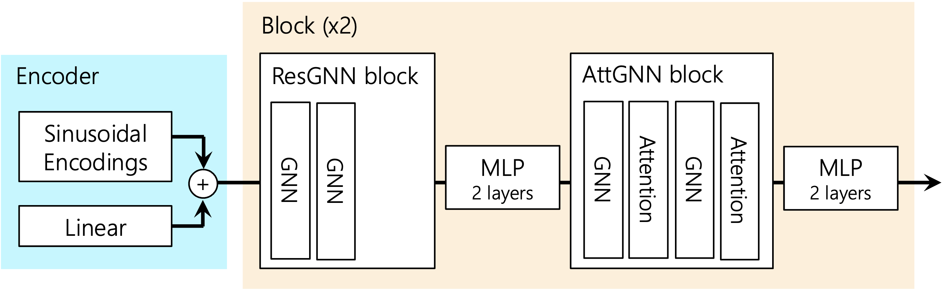
Figure 2: Diagram of our denoising model. Residual connections, edge feature inputs, nonlinearities, and normalization layers have been ommitted for clarity.

We developed a novel architecture for the denoising model, shown in Figure 2. We highlight below several key elements of our design that we found to be important for the placement task:

Interleaved GNN and Attention Layers

We use the message-passing GNN layers for their computational efficiency in capturing node neighborhood information, while the interleaved attention [26] layers address the oversmoothing problem in GNNs by allowing information transfer between nodes that are distant in the netlist graph, but close on the 2D canvas. We find that combining the two types of layers is critical, and significantly outperforms using either type alone.

MLP Blocks

We found (see Section 5.5) that inserting residual 2-layer MLP blocks between each GNN and Attention block improved performance significantly for a negligible increase in computation time.

Sinusoidal 2D Encodings

The model receives 2D sinusoidal position encodings, in addition to the original $(x,y)$ coordinates, as input. We find (see Section 5.5) that this improves the precision with which the model places small objects.

In this work, we use 3 sizes of models: Small, Med, and Big, with 233k, 1.23M, and 4.60M parameters respectively. Model hyperparameters can be found in Appendix A.

4.2 Guided Sampling

One of the key advantages of using diffusion models is the ability to optimize for downstream objectives through guided sampling. We use universal guidance [3] with easily computed potential functions to improve the HPWL and legality of generated samples without training additional models. The guidance potential $\varphi(x)$ is defined as the weighted sum $w_{\text{legality}}\cdot\varphi_{\text{legality}}+w_{\text{hpwl}}\cdot\varphi_{\text{hpwl}}$ of potentials for each of our optimization objectives.

The legality potential $\varphi_{\text{legality}}(x)$ for a netlist with objects $V$ is given by:

$$\varphi_{\text{legality}}(x)=\sum_{i,j\in V}\text{min}(0,{d_{ij}(x)})^{2}$$ (2)

where $d_{i}j$ is the signed distance between objects $i$ and $j$, which we can compute easily for rectangular objects. Note that the summand is $0$ for any pair of non-overlapping objects, and increases as overlap increases.

We define $\varphi_{\text{hpwl}}(x)$ simply as the HPWL of the placement $x$. We compute this in a parallelized, differentiable manner by casting HPWL computation in terms of the message-passing framework used in GNNs [27] and implementing a custom GNN layer with no learnable parameters in PyG [28].

Instead of gradients from a classifier [29], we follow Bansal et al. [3] in using $g(x_{t})=\nabla_{x_{t}}\varphi(\hat{x}_{0})$, where $\hat{x}_{0}$ is the prediction of $x_{0}$ based on the denoising model’s output at time step $t$. The combined diffusion score is then given by $f_{\theta}(x_{t})+g(x_{t})$.

4.3 Datasets

We obtain datasets (Table 1) consisting of tuples $(x,c)$ using different two methods, outlined below.

4.3.1 Generated dataset

We utilize ArtNetGen [30] to produce an artificial netlist and map the nodes to an open-source ASAP7 PDK [31], then we adapt it to include realistic SRAM macros. The Cadence EDA tool then performs concurrent placement of the macros and standard cells. This produces realistic, legal, and near-optimal placements, but is slow. To combat this, the netlist generation and placement occur in parallel and the clock optimization, routing, and power cell placement steps are removed from the Cadence flow. Although these steps can affect final component placements, their optimizations are to be performed in evaluation after we initialize the placement. Currently, the flow still takes 15 minutes to generate a single sample of around 100 macros and 15k instances. Thus, to further improve the number of realistic samples, we augment the final placements by performing legal transformations.

4.3.2 Synthetic dataset

To generate larger datasets, we randomly generate objects (sizes sampled from uniform distribution), and place them at random, ensuring legality by retrying if objects overlap. Following Rent’s Rule [32], we then sample a number of pins for each object using a power law. Next, we generate edges between pins by sampling independently from $\text{Bernoulli}(p)$ for each pair of pins on different objects. To approximate the structure of real circuits, we have $p$ decay exponentially with L1 distance between the pins connected by the edge. This method, depicted in Figure 3 allows us to generate ~100k “circuits” each containing ~200 objects in a day using 32 CPUs.

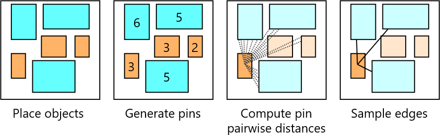
Figure 3: Visualization of the steps involved in generating synthetic data.

We vary $p$, as well as several other parameters, to generate synthetic datasets SynthM and SynthM-Short with different levels of wirelength optimality. Notice that the wires in SynthM are, on average, much longer than those in SynthM-Short, corresponding to placements that are less HPWL-optimal. A detailed list of data generation parameters can be found in Appendix A.

Table 1: Parameters of datasets used.

Name	#Train	#Validation	Objects	Edges	HPWL
SynthM	95000	5000	230	1400	132
SynthM-Short	95000	5000	230	1000	34
SynthL	12000	600	1000	5500	330

4.4 Implementation

We evaluate the performance of our model on circuits presented in two sets of public benchmarks, ISPD2005 [33] and ICCAD04 [34]. Our models are implemented using Pytorch [35] and Pytorch-Geometric [28], and train on machines with 8 Intel Xeon Gold 6330 CPU cores, using a single Nvidia RTX A5000 GPU. We pre-train our models using the Adam optimizer [36] for 3M steps, with 100k steps of fine-tuning where applicable.

5 Results

5.1 Model Performance

Table 2: Results for models trained on various datasets. Values are averages over 128 samples.

	SynthM			SynthL
Model	Small	Med	Big	Small	Med	Big
#Params	0.23M	1.23M	4.60M	0.23M	1.23M	4.60M
Legality	0.936	0.961	0.966	0.901	0.914	0.942
HPWL Ratio	1.026	1.016	1.020	1.075	1.037	1.014

Table 2 shows evaluation results on SynthM and SynthL datasets. In all cases, the model achieves legality better than $0.9$, with HPWL ratio (of diffusion-sampled to original placements) very close to 1. This validates our model design, and shows that our model is capable of learning approximately-correct, near-optimal placements in both realistic and synthetic circuits. Examples of generated samples are shown in Table 3

More importantly, our experiments with different model sizes on SynthM show significant increases in performance as model size increases over a modest range, with HPWL ratio decreasing and legality increasing with bigger models. This is an encouraging result, suggesting that not only does our model obtain lower loss with increasing size, but that evaluation metrics, such as legality, improve too.

It is also worth noting that performance deteriorates with larger circuits, as shown in Table 2. This is likely due to the precision required to place many small objects without overlaps, and suggests that larger models are needed to tackle larger circuits (benchmark circuits have thousands of objects). The data and compute required to train such models on large examples presents a significant challenge, which we address in Section 5.2.

Table 3: Selection of SynthM placements generated by Med Model.

Legality	0.976	0.964	0.942
HPWL Ratio	1.031	1.043	1.021

5.2 Unsupervised Pre-training

Because of the difficulty in generating realistic netlists and placements with many objects, we propose the following approach, inspired by LLM training: we first train on a large set of small-circuit synthetic data (which is easily generated), then fine-tune on a much smaller set of large-circuit examples, which can be either synthetic or real. In this section we investigate the usefulness of this approach, examining the performance of models pre-trained on SynthM when deployed on SynthL in the zero-shot and fine-tuned settings.

5.2.1 Zero-shot and Fine-tuned Performance

We see from our results in Table 4 that models of all sizes exhibit decent zero-shot performance on SynthL, despite only training on netlists with far fewer objects. With only a small amount of fine-tuning, performance improves dramatically, with the Big model achieving $>0.95$ legality and HPWL close to the training distribution. Moreover, we observe that the favorable scaling properties of our models apply to the zero-shot and fine-tuned settings as well, with performance increasing substantially with increased model size.

Table 4: Evaluation on SynthL of models pre-trained on SynthM in zero-shot and fine-tuned settings. HPWL ratio and legality are averages over 128 samples.

	Zero-shot			Fine-tuned
Model	Small	Med	Big	Small	Med	Big
Legality	0.867	0.878	0.898	0.917	0.935	0.951
HPWL Ratio	1.302	1.241	1.176	1.057	1.047	1.018

5.2.2 Impact of Pre-training Dataset

We also investigated the relative effectiveness of pre-training on different datasets.

Table 5: Zero-shot evaluation on SynthL of Med-size model, pre-trained on various datasets.

Pre-training Dataset	SynthM			SynthM-Short
Model	Small	Med	Big	Small	Med	Big
Legality	0.867	0.878	0.898	0.798	0.810	0.796
HPWL Ratio	1.302	1.241	1.176	1.065	1.104	0.993

Running zero-shot evaluations on SynthL, we find in Table 5 that pre-training on the more-optimized SynthM-Short does lead to significantly better zero-shot HPWL than SynthM. However, the improved HPWL comes at the expense of legality, where SynthM-Short performs almost $10\%$ worse. Note that HPWL tends to improve as legality degrades, since overlapping objects minimize wirelengths better than non-overlapping ones. This indicates that pre-training on synthetic datasets with shorter wirelengths (and therefore more optimal placements) do not produce significantly better models than datasets with longer wirelengths. One possible reason for this is that because of the increased decay of $p$ over distance in SynthM-Short, objects have to be much closer to each other than in SynthM to have a reasonable chance of being connected. While this can allow the model to better optimize HPWL, it also restricts the flow of information within the GNN layers and could result in poorer representations being learned. This effect could be especially detrimental when attempting zero-shot transfer to other datasets or real circuits that contain edges between distant objects due to functional requirements.

Our finding stands in contrast to prior work on generating synthetic data [18], which proposes generating data that is optimal with respect to swaps between objects.

5.3 Guided Sampling

As shown in Table 6, guidance significantly improves legality and HPWL during zero-shot sampling, with up to a $14\%$ improvement in legality for models pre-trained on SynthM-Short. Moreover, we find that adding HPWL guidance improves wirelength significantly without deteriorating legality. This result shows that our guidance method is effective in optimizing generated samples without requiring additional training.

Table 6: Zero-shot evaluations on SynthL of Med-size models in 3 sampling modes: no guidance; only legality guidance; both legality and HPWL. Values are averages over 32 samples.

Pre-training dataset	SynthM			SynthM-Short
Guidance	None	Legality Only	Both	None	Legality Only	Both
Legality	0.883	0.965	0.970	0.812	0.948	0.950
HPWL Ratio	1.239	1.317	1.211	1.119	1.217	1.151

5.4 Placing Real-World Circuits

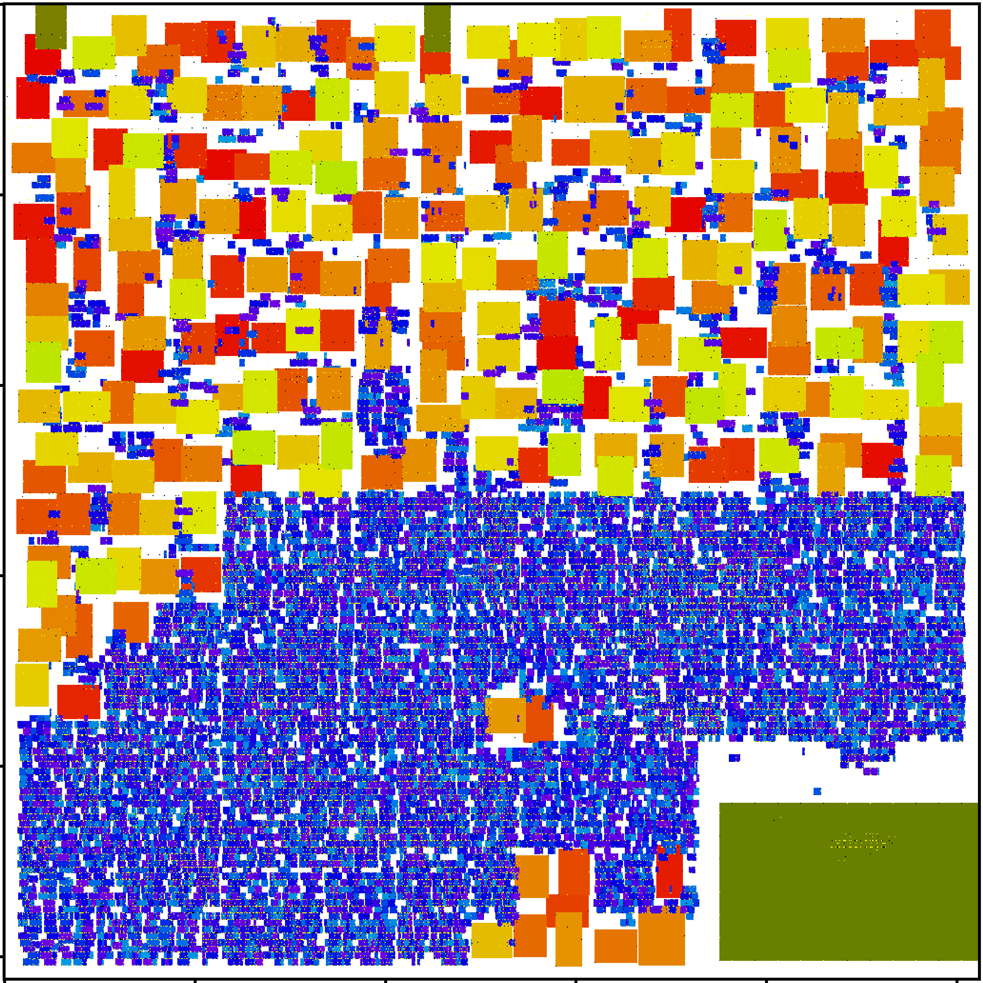
(a) Original Circuit

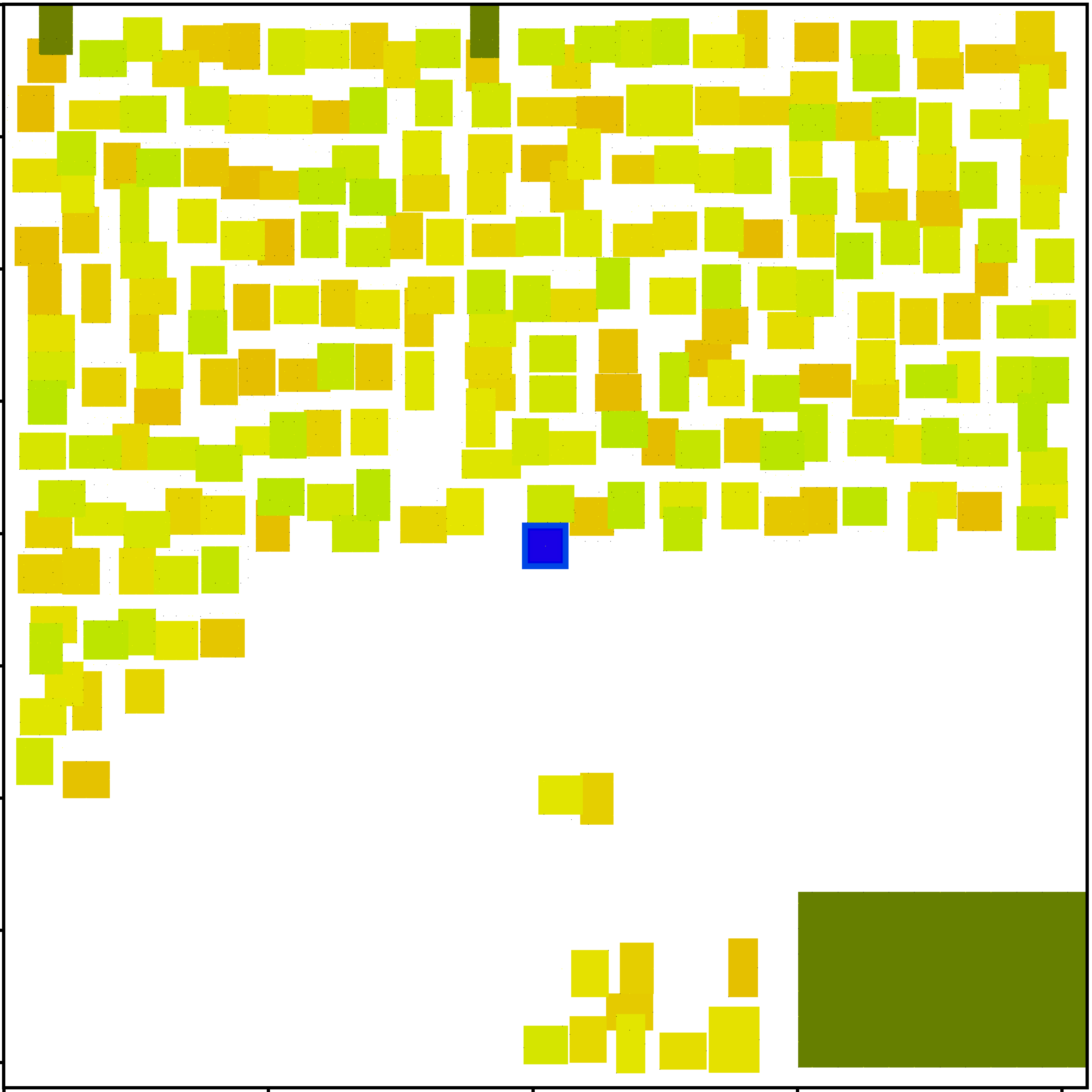
(b) After Clustering

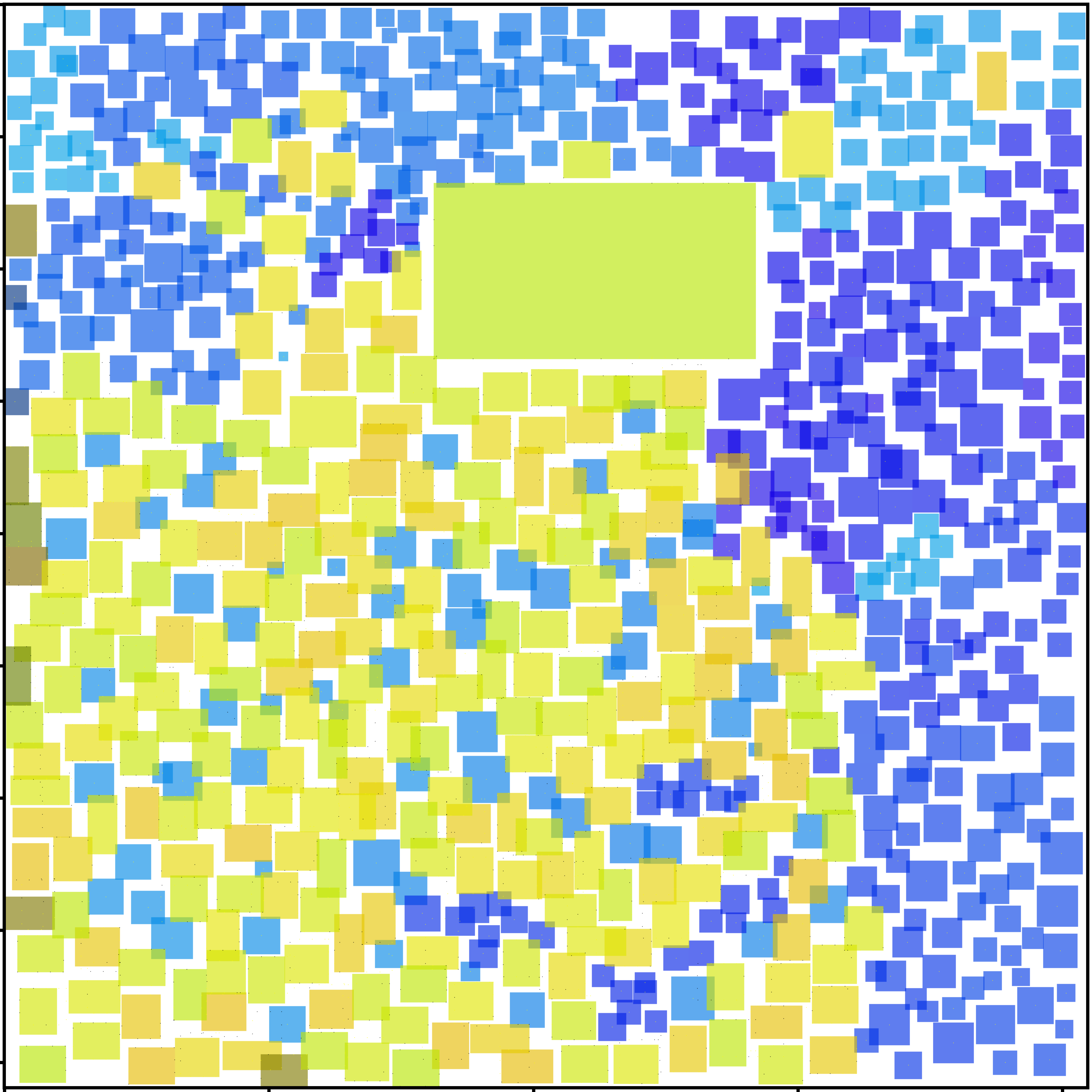
(c) Diffusion-based Placement

Figure 4: We perform mixed-size placement on a circuit in the IBM Mixed Size benchmark. Note that the placement information from (a) is for visualization only, and not used by the model when sampling.

(a) Phase 1

(b) Phase 2

(c) DREAMPlace

Figure 5: Comparison between our placements and DREAMPlace on Adaptec3

Our experiments with synthetic datasets show that diffusion models have great potential for tackling the placement problem. We focus in particular on the mixed-size placement problem, which requires us to place several hundred large macros, as well as many (potentially hundreds of thousands) small standard cells. This is an incredibly challenging problem, and would require prohibitively large computational resources to solve with a diffusion model alone. Therefore, we follow Mirhoseini et al. [1] in first clustering the standard cells to reduce their number to a manageable level, and then use the diffusion model to generate a near-optimal placement for the macros and the clusters. For the following, we use a Med model pre-trained on SynthM with no fine-tuning, and with both legality and HPWL guidance.

We find that our model, which has been entirely trained on synthetic data, shows reasonable zero-shot transfer to real-world circuits. As seen in Figure 4(c), it is able to place the densely-connected standard cell clusters (blue) and macros (yellow) together, with cell clusters on the top and right edges of the canvas, while placing the large rectangular macro along the interface between the two groups.

To enable mixed-sized placements, we employ a simplified 2-stage workflow, comparable to previous works [2, 1]. Step 1 of the simplified workflow calls the diffusion model to place each one of the macros and clusters, unclustering the standard cells to be in the center of their respective clusters. Step 2 runs global placement using DREAMPlace initialized on positions laid out in step 1, obtaining the final mixed-sized placement result.

We present our evaluation results in Table 8, and show that in most cases we improve the placement quality of DREAMPlace while saving runtime. We observe that DREAMPlace is extremely sensitive to initialization and that the placement quality varies from run to run. We therefore ran our evaluation on the seed 1000, and report the average over 5 runs. As shown in Figure 5(b), we observe that while DREAMPlace concurrently moves the macros and standard cells, the relative bias of the initialization is preserved after phase 2. This shows the efficacy of our initialization in that it does impact the final placement quality. Furthermore, for certain samples in the ICCAD2004 benchmark (ibm02, ibm03, ibm04), DREAMPlace sometimes fails to converge to the density requirement, causing high iteration counts. We find that our workflow avoids this behavior, stabilizing the runtime.

Table 7: Mixed Placement Workflow

Phase	Operation	Description
1	Cluster Placement	Places macros and standard cells with diffusion
2	GP (with DREAMPlace)	Run global placement with initialization

Table 8: Mixed Placement Results

	HPWL x $10^{6}$		Iterations
Benchmark	DREAMPlace	Ours	DREAMPlace	Ours
Adaptec1	68.4	67.3 $\pm 0.1$ -1.61%	740	646 $\pm 2$ -12.8%
Adaptec2	86.5	78.6 $\pm 1.2$ -9.92%	863	698 $\pm 2$ -19.2%
Adaptec3	139.3	134 $\pm 0.12$ -3.81%	955	$663$ $\pm 1$ -33.8%
Adaptec4	139.0	133.4 $\pm 0.32$ -4.03%	913	663$\pm 1$ -27.3%
ibm01	2.56	2.55 $\pm 0.2$-0.04%	702	560 $\pm 4$ -20.3%
ibm02	5.25	5.11 $\pm 0.7$ -2.66%	1076	534 $\pm 4$ -50.4%
ibm03	8.37	8.16 $\pm 0.2$ -2.51%	1449	548 $\pm 2$ -62.2%
ibm04	105.3	94.5 $\pm 3.2$-10.3%	1123	594 $\pm 4$ -47.2%
ibm06	5.94	5.77 $\pm 0.02$ -2.87%	676	523 $\pm 7$ -22.7%

5.5 Ablations

Table 9: Ablations of Med model on SynthM. Values are averages over 32 samples.

	Complete Model	No Input Encoding	No MLP Blocks	No Att Layers
Legality	0.960	0.943	0.938	0.890
HPWL Ratio	1.021	1.025	1.026	1.013

Ablations over several elements of our model architecture are shown in Table 9. When either the sinusoidal encodings or MLP blocks are removed, the model performs substantially worse in both legality and HPWL. Removing attention layers also causes sample quality to plummet, as evidenced by poor legality scores. This demonstrates the importance of these components to model performance.

6 Limitations

While we found that synthetic datasets with shorter wirelengths can cause models to transfer more poorly to out-of-distribution circuits, we believe more work can be done to investigate the effects of other parameters such as the distribution of object sizes.

Another limitation lies in the reliance on guidance to optimize generated samples. While guidance is effective and flexible, it functions by biasing the model to sample from a subset of the training distribution. This fundamentally limits the HPWL that can be achieved. Exploring other optimization methods that involve fine-tuning the model, such as reward-weighted regression or DDPO [37], is a promising area for future work.

Like previous methods, our model relies on a final optimizer to complete mixed-sized placements of millions of cells. The quality of this optimizer will inevitably influence the final quality of placement.

7 Conclusion

In this work, we explored an approach that departs from many existing methods for tackling macro placement: using diffusion models to generate placements. To train and apply such models at scale, we developed a novel neural network architecture, as well as a synthetic data generation algorithm. We show that our models generalize to new circuits, and when combined with guided sampling, can generate optimized placements even on large, real-world circuit benchmarks.

Despite the success of our guidance method, we believe significant improvements can be made in optimizing the generated samples through further training with DDPO, or fine-tuning on realistic circuit datasets.

In conclusion, we find that pre-training diffusion models on synthetic data is a promising approach, with our models generating competitive placements despite never having trained on realistic circuit data. We hope that our results inspire further work in this area.

Appendix A Implementation Details

Hyperparameters for our model are listed in Table 10. We used the linear noise schedule and DDPM formulation found in Ho et al. [25]. We also list parameters for generating our synthetic datasets in Table 11.

Table 10: Hyperparameters for our models. We refer the reader to our code for more details.

	Small	Med	Big
Model Dimensions
Model size	64	128	256
Blocks	2
Layers per block	2	2	3
AttGNN size	32	32	256
ResGNN size	64	256	256
MLP size factor	4
MLP layers per block	2
Input Encodings
Timestep encoding dimension	32
Input encoding dimension	32
GNN Layers
Type	GATv2[38]
Heads	4
Guidance Parameters
Legality weight	2.0
HPWL weight	0.0005

Table 11: Parameters for generating our synthetic data. Unless otherwise stated, SynthM-Short and SynthL use the same parameters as SynthM. We refer the reader to our code for more details. Note that sizes and distances are normalized so that a value of $2$ corresponds to the width of the canvas.

	SynthM	SynthM-Short	SynthL
Stop Density Distribution
Distribution type	Uniform
Low	0.75
High	0.9
Aspect Ratio Distribution
Distribution type	Uniform
Low	0.25		0.2
High	1.0
Object Size Distribution
Distribution type	Clipped Exponential
Scale	0.08		0.04
Max	1.0		0.8
Min	0.02		0.025
Edge Distribution
Distribution type	Bernoulli, $p$ decays exp.
Scale	0.15	$0.2\cdot(\text{Instance size})$	0.1
Max $p$	0.216	0.9	0.216
Multiplier	0.27	1.2	0.27

Appendix B Additional Details of Benchmarks

We show the statistical distribution of our mixed placement workload in Table 12. We have removed the ibm05 benchmark as it contains only standard cells.

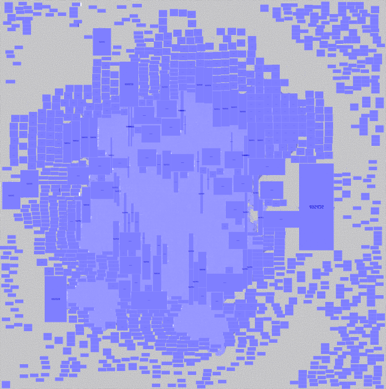
(a) Phase 2

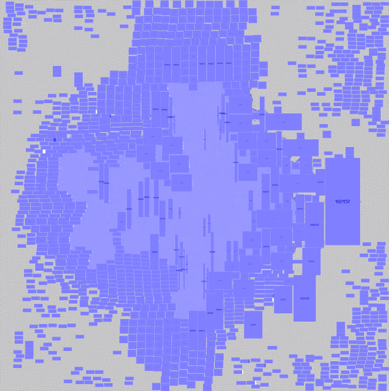
(b) DREAMPlace

Figure 6: Comparison between our placements and DREAMPlace on Adaptec4

Table 12: Statistics of different chip benchmarks.

Benchmark	Hard Macros	Standard Cells	Nets	Pins	Ports	Util(%)
adaptec1	63	210,904	3,709	4,768	0	55.62
adaptec2	190	254,457	4,346	10,663	0	74.46
adaptec3	201	450,927	6,252	11,521	0	61.51
adaptec4	92	494,716	5,939	13,720	0	48.62
ibm01	246	12,506	908	1,928	246	61.94
ibm02	272	19,321	602	1,466	259	64.63
ibm03	290	22,846	614	1,237	283	57.97
ibm04	296	26,899	1,512	3,167	287	54.88
ibm06	178	32,320	83	175	166	54.77

References

- Mirhoseini et al. [2020] Azalia Mirhoseini, Anna Goldie, Mustafa Yazgan, Joe W. J. Jiang, Ebrahim M. Songhori, Shen Wang, Young-Joon Lee, Eric Johnson, Omkar Pathak, Sungmin Bae, Azade Nazi, Jiwoo Pak, Andy Tong, Kavya Srinivasa, William Hang, Emre Tuncer, Anand Babu, Quoc V. Le, James Laudon, Richard Ho, Roger Carpenter, and Jeff Dean. Chip placement with deep reinforcement learning. CoRR, abs/2004.10746, 2020. URL https://arxiv.org/abs/2004.10746.
- Lai et al. [2023] Yao Lai, Jinxin Liu, Zhentao Tang, Bin Wang, Jianye Hao, and Ping Luo. Chipformer: Transferable chip placement via offline decision transformer. In International Conference on Machine Learning, ICML 2023, 23-29 July 2023, Honolulu, Hawaii, USA, volume 202 of Proceedings of Machine Learning Research, pages 18346–18364. PMLR, 2023. URL https://proceedings.mlr.press/v202/lai23c.html.
- Bansal et al. [2023] Arpit Bansal, Hong-Min Chu, Avi Schwarzschild, Soumyadip Sengupta, Micah Goldblum, Jonas Geiping, and Tom Goldstein. Universal guidance for diffusion models, 2023.
- Adya et al. [2004] S.N. Adya, S. Chaturvedi, J.A. Roy, D.A. Papa, and I.L. Markov. Unification of partitioning, placement and floorplanning. In IEEE/ACM International Conference on Computer Aided Design, 2004. ICCAD-2004., pages 550–557, 2004. doi: 10.1109/ICCAD.2004.1382639.
- Adya and Markov [2002] Saurabh N. Adya and Igor L. Markov. Consistent placement of macro-blocks using floorplanning and standard-cell placement. In Proceedings of the 2002 International Symposium on Physical Design, ISPD ’02, page 12–17, New York, NY, USA, 2002. Association for Computing Machinery. ISBN 1581134606. doi: 10.1145/505388.505392. URL https://doi.org/10.1145/505388.505392.
- Nam et al. [2005a] Gi-Joon Nam, Charles J. Alpert, Paul Villarrubia, Bruce Winter, and Mehmet Yildiz. The ispd2005 placement contest and benchmark suite. In Proceedings of the 2005 International Symposium on Physical Design, ISPD ’05, page 216–220, New York, NY, USA, 2005a. Association for Computing Machinery. ISBN 1595930213. doi: 10.1145/1055137.1055182. URL https://doi.org/10.1145/1055137.1055182.
- Mirhoseini et al. [2021] Azalia Mirhoseini, Anna Goldie, Mustafa Yazgan, Joe Wenjie Jiang, Ebrahim Songhori, Shen Wang, Young-Joon Lee, Eric Johnson, Omkar Pathak, Azade Nazi, et al. A graph placement methodology for fast chip design. Nature, 594(7862):207–212, 2021.
- Yue et al. [2022] Summer Yue, Ebrahim M. Songhori, Joe Wenjie Jiang, Toby Boyd, Anna Goldie, Azalia Mirhoseini, and Sergio Guadarrama. Scalability and generalization of circuit training for chip floorplanning. In Proceedings of the 2022 International Symposium on Physical Design, ISPD ’22, page 65–70, New York, NY, USA, 2022. Association for Computing Machinery. ISBN 9781450392105. doi: 10.1145/3505170.3511478. URL https://doi.org/10.1145/3505170.3511478.
- Cheng et al. [2023] Chung-Kuan Cheng, Andrew B. Kahng, Sayak Kundu, Yucheng Wang, and Zhiang Wang. Assessment of reinforcement learning for macro placement. In Proceedings of the 2023 International Symposium on Physical Design, ISPD ’23, page 158–166, New York, NY, USA, 2023. Association for Computing Machinery. ISBN 9781450399784. doi: 10.1145/3569052.3578926. URL https://doi.org/10.1145/3569052.3578926.
- Cheng and Yan [2021] Ruoyu Cheng and Junchi Yan. On joint learning for solving placement and routing in chip design, 2021.
- Lai et al. [2022] Yao Lai, Yao Mu, and Ping Luo. Maskplace: Fast chip placement via reinforced visual representation learning. In S. Koyejo, S. Mohamed, A. Agarwal, D. Belgrave, K. Cho, and A. Oh, editors, Advances in Neural Information Processing Systems, volume 35, pages 24019–24030. Curran Associates, Inc., 2022. URL https://proceedings.neurips.cc/paper_files/paper/2022/file/97c8a8eb0e5231d107d0da51b79e09cb-Paper-Conference.pdf.
- Gu et al. [2024] Hao Gu, Jian Gu, Keyu Peng, Ziran Zhu, Ning Xu, Xin Geng, and Jun Yang. Lamplace: Legalization-aided reinforcement learning based macro placement for mixed-size designs with preplaced blocks. IEEE Transactions on Circuits and Systems II: Express Briefs, pages 1–1, 2024. doi: 10.1109/TCSII.2024.3375068.
- Chen et al. [2023] Yifan Chen, Jing Mai, Xiaohan Gao, Muhan Zhang, and Yibo Lin. Macrorank: Ranking macro placement solutions leveraging translation equivariancy. In Proceedings of the 28th Asia and South Pacific Design Automation Conference, ASPDAC ’23, page 258–263, New York, NY, USA, 2023. Association for Computing Machinery. ISBN 9781450397834. doi: 10.1145/3566097.3567899. URL https://doi.org/10.1145/3566097.3567899.
- Zheng et al. [2023a] Su Zheng, Lancheng Zou, Siting Liu, Yibo Lin, Bei Yu, and Martin Wong. Mitigating distribution shift for congestion optimization in global placement. In 2023 60th ACM/IEEE Design Automation Conference (DAC), pages 1–6, 2023a. doi: 10.1109/DAC56929.2023.10247660.
- Zheng et al. [2023b] Su Zheng, Lancheng Zou, Peng Xu, Siting Liu, Bei Yu, and Martin Wong. Lay-net: Grafting netlist knowledge on layout-based congestion prediction. In 2023 IEEE/ACM International Conference on Computer Aided Design (ICCAD), pages 1–9. IEEE, 2023b.
- Wang et al. [2022] Bowen Wang, Guibao Shen, Dong Li, Jianye Hao, Wulong Liu, Yu Huang, Hongzhong Wu, Yibo Lin, Guangyong Chen, and Pheng Ann Heng. Lhnn: Lattice hypergraph neural network for vlsi congestion prediction. In Proceedings of the 59th ACM/IEEE Design Automation Conference, pages 1297–1302, 2022.
- Ghose et al. [2021] Amur Ghose, Vincent Zhang, Yingxue Zhang, Dong Li, Wulong Liu, and Mark Coates. Generalizable cross-graph embedding for gnn-based congestion prediction. In 2021 IEEE/ACM International Conference On Computer Aided Design (ICCAD), pages 1–9. IEEE, 2021.
- Liu et al. [2022a] Yiting Liu, Ziyi Ju, Zhengming Li, Mingzhi Dong, Hai Zhou, Jia Wang, Fan Yang, Xuan Zeng, and Li Shang. Floorplanning with graph attention. In Proceedings of the 59th ACM/IEEE Design Automation Conference, DAC ’22, page 1303–1308, New York, NY, USA, 2022a. Association for Computing Machinery. ISBN 9781450391429. doi: 10.1145/3489517.3530484. URL https://doi.org/10.1145/3489517.3530484.
- Liu et al. [2022b] Yiting Liu, Ziyi Ju, Zhengming Li, Mingzhi Dong, Hai Zhou, Jia Wang, Fan Yang, Xuan Zeng, and Li Shang. Graphplanner: Floorplanning with graph neural network. ACM Trans. Des. Autom. Electron. Syst., 28(2), dec 2022b. ISSN 1084-4309. doi: 10.1145/3555804. URL https://doi.org/10.1145/3555804.
- Kingma and Welling [2022] Diederik P Kingma and Max Welling. Auto-encoding variational bayes, 2022.
- Lin et al. [2019] Yibo Lin, Shounak Dhar, Wuxi Li, Haoxing Ren, Brucek Khailany, and David Z. Pan. Dreampiace: Deep learning toolkit-enabled gpu acceleration for modern vlsi placement. In 2019 56th ACM/IEEE Design Automation Conference (DAC), pages 1–6, 2019.
- Chen et al. [2006] Tung-chieh Chen, Zhe-wei Jiang, Tien-chang Hsu, Hsin-chen Chen, and Yao-wen Chang. A high-quality mixed-size analytical placer considering preplaced blocks and density constraints. In 2006 IEEE/ACM International Conference on Computer Aided Design, pages 187–192, 2006. doi: 10.1109/ICCAD.2006.320084.
- Kahng and Reda [2006] Andrew B Kahng and Sherief Reda. A tale of two nets: Studies of wirelength progression in physical design. In Proceedings of the 2006 international workshop on System-level interconnect prediction, pages 17–24, 2006.
- Song et al. [2021] Yang Song, Jascha Sohl-Dickstein, Diederik P. Kingma, Abhishek Kumar, Stefano Ermon, and Ben Poole. Score-based generative modeling through stochastic differential equations, 2021.
- Ho et al. [2020] Jonathan Ho, Ajay Jain, and Pieter Abbeel. Denoising diffusion probabilistic models, 2020.
- Vaswani et al. [2017] Ashish Vaswani, Noam Shazeer, Niki Parmar, Jakob Uszkoreit, Llion Jones, Aidan N Gomez, Łukasz Kaiser, and Illia Polosukhin. Attention is all you need. Advances in neural information processing systems, 30, 2017.
- Gilmer et al. [2017] Justin Gilmer, Samuel S. Schoenholz, Patrick F. Riley, Oriol Vinyals, and George E. Dahl. Neural message passing for quantum chemistry, 2017.
- Fey and Lenssen [2019] Matthias Fey and Jan E. Lenssen. Fast graph representation learning with PyTorch Geometric. In ICLR Workshop on Representation Learning on Graphs and Manifolds, 2019.
- Dhariwal and Nichol [2021] Prafulla Dhariwal and Alex Nichol. Diffusion models beat gans on image synthesis. CoRR, abs/2105.05233, 2021. URL https://arxiv.org/abs/2105.05233.
- Kim et al. [2023] Daeyeon Kim, Sung-Yun Lee, Kyungjun Min, and Seokhyeong Kang. Construction of realistic place-and-route benchmarks for machine learning applications. IEEE Transactions on Computer-Aided Design of Integrated Circuits and Systems, 42(6):2030–2042, 2023. doi: 10.1109/TCAD.2022.3209530.
- Clark et al. [2016] Lawrence T. Clark, Vinay Vashishtha, Lucian Shifren, Aditya Gujja, Saurabh Sinha, Brian Cline, Chandarasekaran Ramamurthy, and Greg Yeric. Asap7: A 7-nm finfet predictive process design kit. Microelectronics Journal, 53:105–115, 2016. ISSN 0026-2692. doi: https://doi.org/10.1016/j.mejo.2016.04.006. URL https://www.sciencedirect.com/science/article/pii/S002626921630026X.
- Lanzerotti et al. [2005] M. Y. Lanzerotti, G. Fiorenza, and R. A. Rand. Microminiature packaging and integrated circuitry: The work of e. f. rent, with an application to on-chip interconnection requirements. IBM Journal of Research and Development, 49(4.5):777–803, 2005. doi: 10.1147/rd.494.0777.
- Nam et al. [2005b] Gi-Joon Nam, C.J. Alpert, Paul Villarrubia, Bruce Winter, and Mehmet Yildiz. The ispd2005 placement contest and benchmark suite. pages 216–220, 04 2005b. doi: 10.1145/1055137.1055182.
- icc [2004] Iccad 2004. international conference on computer aided design (ieee cat. no.04ch37606). In IEEE/ACM International Conference on Computer Aided Design, 2004. ICCAD-2004., pages 0, 1–, 2004. doi: 10.1109/ICCAD.2004.1382513.
- Paszke et al. [2019] Adam Paszke, Sam Gross, Francisco Massa, Adam Lerer, James Bradbury, Gregory Chanan, Trevor Killeen, Zeming Lin, Natalia Gimelshein, Luca Antiga, et al. Pytorch: An imperative style, high-performance deep learning library. Advances in neural information processing systems, 32, 2019.
- Kingma and Ba [2014] Diederik P Kingma and Jimmy Ba. Adam: A method for stochastic optimization. arXiv preprint arXiv:1412.6980, 2014.
- Black et al. [2024] Kevin Black, Michael Janner, Yilun Du, Ilya Kostrikov, and Sergey Levine. Training diffusion models with reinforcement learning, 2024.
- Brody et al. [2022] Shaked Brody, Uri Alon, and Eran Yahav. How attentive are graph attention networks?, 2022.