In-Context Probing Approximates Influence Function for Data Valuation

Abstract

Data valuation quantifies the value of training data, and is used for data attribution (i.e., determining the contribution of training data towards model predictions), and data selection; both of which are important for curating high-quality datasets to train large language models. In our paper, we show that data valuation through in-context probing (i.e., prompting a LLM) approximates influence functions for selecting training data. We provide a theoretical sketch on this connection based on transformer models performing “implicit" gradient descent on its in-context inputs. Our empirical findings show that in-context probing and gradient-based influence frameworks are similar in how they rank training data. Furthermore, fine-tuning experiments on data selected by either method reveal similar model performance.

In-Context Probing Approximates Influence Function for Data Valuation

Cathy Jiao¹  Gary Gao²  Chenyan Xiong^{1 1} Language Technologies Institute, Carnegie Mellon University ² School of Computer Science, Carnegie Mellon University {cljiao, wgao2, cx}@cs.cmu.edu

1 Introduction

Data valuation using in-context probing (ICP) – prompting a LLM to determine the quality of a training data sample – has become an important avenue for curating high-quality training data Rubin et al. (2022); Nguyen and Wong (2023); Wettig et al. (2024). However, it is unclear why in-context probing is effective at training data valuation since there are multiple factors to consider for evaluating the quality of training data: for instance, mixtures, utility, and the quantity of data Lee et al. (2022); Xie et al. (2023); Goyal et al. (2024).

In our paper, we offer an explanation to this phenomena by drawing connections between ICP and influence functions Koh and Liang (2017). Theoretically, we connect these two frameworks by showing that they both approximate change in loss on a test task; with ICP taking an “implicit" gradient descent step on a training sample Von Oswald et al. (2023); Dai et al. (2023). Empirically, we observe that in-context probing and gradient-based data valuation methods correlate in their rankings of training data for instruction-following tasks. Furthermore, fine-tuning on smaller subsets of highly-ranked data scored by either method resulted in better model performance compared to fine-tuning on larger amounts of data. Finally, fine-tuning on data placed by either method in the same data rank resulted in similar model performance in general.

Overall, our findings suggest that ICP may serve as a proxy for influence function data valuation under certain settings (i.e., data selection for fine-tuning). While future work can explore different settings, this direction has some useful implications. Data valuation through ICP is cost effective, and can even be done through API calls. In contrast, gradient-based data valuation methods – such as influence functions – require access to model parameters, and are computationally expensive.

2 Related Work

Obtaining high-quality training data is important for improving model learning and reducing training costs Lee et al. (2022); Sorscher et al. (2023); Ye et al. (2024); Albalak et al. (2024). One avenue for training data valuation is influence functions Koh and Liang (2017), which estimates the influence of a training sample on model predictions upon adding/removing it from the train set. Despite being computationally expensive in LLM settings Grosse et al. (2023), these methods are effective for curating subsets of high-quality training data Pruthi et al. (2020); Park et al. (2023); Han et al. (2023); Xia et al. (2024); Engstrom et al. (2024).

Simultaneously, recent works have also leveraged ICP for training data valuation Rubin et al. (2022); Nguyen and Wong (2023); Iter et al. (2023); Wettig et al. (2024). These methods involve measuring the model output likelihoods of task given an in-context train sample, or prompting an LLM with questions to identity high-quality training samples.

Since both influence function methods and ICP methods may be used for data valuation, a key component to connecting these ideas lies in a recent body of work which suggest that in-context learning implicitly performs gradient descent by constructing meta-gradients Von Oswald et al. (2023); Dai et al. (2023). Other frameworks exist for understanding in-context learning mechanisms exist. For instance, Xie et al. (2021) states that in-context learning arises from implicit Bayesian inference due to latent concepts learned during pretraining, and Olsson et al. (2022) attributes in-context learning to induction heads. In our work, focus our attention on the first framework in order to draw connections between ICP and influence functions.

3 Preliminaries

In this section, we introduce and formalize frameworks for data valuation through in-context probing and influence functions.

3.1 In-Context Data Valuation

While multiple works have examined data selection using in-context learning abilities of LLMs Nguyen and Wong (2023); Wettig et al. (2024); Chen et al. (2024); Li et al. (2024a), the method we focus on is the an one-shot ICP quality score introduced in Li et al. (2024b), which was used to curate high-quality instruction-tuning data. Given a dataset of tasks $\mathcal{D}=\{x_{1},...,x_{n}\}$, each task $x_{i}=[x_{i}^{q};x_{i}^{a}]$ is composed of a query, $x_{i}^{q}$, and an answer, $x_{i}^{a}$. Let $\theta$ be the parameters of the LLM used for scoring. Then the zero-shot score of task $x_{i}$ is:

$$\text{s}_{\text{zs}}(x_{i};\theta)=\frac{1}{L}\sum_{j=1}^{L}\log p_{\theta}(x_{i,j}^{a}|x^{q},x_{i,<j-1}^{a})$$ (1)

where $x_{i,j}^{a}$ is the $j$ token in $x_{i}^{a}$ and $L$ is the length of $x_{i}^{a}$. Given a candidate instruction $z=[z^{q};z^{a}]$, we use the one-shot score to determine if including $z$ improves the model’s probability of the answer:

$$\text{s}_{\text{os}}(x_{i},z;\theta)=\frac{1}{L}\sum_{j=1}^{L}\log p_{\theta}(x_{j}^{a}|z,x^{q},x_{i,<{j-1}}^{a})$$ (2)

The quality score achieve through ICP reflects the contribution of $z$ for one-shot inference across all tasks in $\mathcal{D}$:

$$\text{ICP}(z,\mathcal{D})=\frac{1}{N}\sum_{i=1}^{N}\mathbbm{1}[s_{os}(x_{i},z;\theta)>s_{zs}(x_{i};\theta)]$$ (3)

3.2 Influence Functions

Influence functions Koh and Liang (2017) approximate changes in model predictions when adding/removing samples from the training data. Given a train sample $z$ from training set $\mathcal{T}$, its influence on a test task $x$ is:

$$\text{Infl}(z,x)=\nabla\mathcal{L}(\theta,x)H^{-1}\nabla\mathcal{L}(\theta,z)$$ (4)

where $H=\frac{1}{N}\sum_{z_{i}\in\mathcal{T}\mathrel{\mathop{\mathchar 58\relax}}i={1,...,N}}\nabla_{\theta}^{2}\mathcal{L}(\theta,z_{i})$ is the Hessian (see Appendix A for full details). However, computing $H^{-1}$ expensive and unstable in non-convex loss function settings, such as for large deep learning models Basu et al. (2021). A simpler and more cost effective alternative is to drop the Hessian and only keep the inner product:

$$\text{Infl}_{\text{IP}}(z,x)=\nabla\mathcal{L}(\theta,x)\cdot\nabla\mathcal{L}(\theta,z)$$ (5)

In particular, Yang et al. (2024) showed that despite dropping the Hessian, $\text{Infl}_{\text{IP}}$ exhibited good order-consistency with Inf. Furthermore, $\text{Infl}_{\text{IP}}$ can also capture the change in loss on a test task $x$ upon training on $z$, as highlighted below:

Lemma 1.

Suppose we have a LLM with parameters $\theta_{t}$. At training iteration $t$, and we perform a stochastic gradient descent with training sample $z$ such that $\theta_{t+1}=\theta_{t}-\eta_{t}\nabla\mathcal{L}(\theta_{t},z)$. Then,

$$\textnormal{Infl}_{\textnormal{IP}}(z,x) =\nabla\mathcal{L}(\theta_{t},x)\cdot\nabla\mathcal{L}(\theta_{t},z)$$

$$\approx\frac{1}{\eta_{t}}\left(\mathcal{L}(x,\theta_{t})-\mathcal{L}(x,\theta_{t+1})\right)$$ (6)

$$\approx\mathcal{L}(x,\theta_{t})-\mathcal{L}(x,\theta_{t+1})$$ (7)

Equation 6 results from a first-order approximation, and holds when $\eta_{t}$ is small: for instance, in fine-tuning settings (see Appendix C for details). If we are interested in $\text{Infl}_{\text{IP}}$ for comparisons (i.e., $\text{Infl}_{\text{IP}}(z_{1},x)$ vs $\text{Infl}_{\text{IP}}(z_{2},x)$), then equation 7 holds assuming that $\eta_{t}$ is consistent across comparisons.

4 Theoretical Analysis

Given the preliminary notes in the previous section, we show how ICP is an approximation of $\text{Infl}_{\text{IP}}$. First, we draw a connection between gradient descent and ICP.

Proposition 1.

Given a LLM with parameters $\theta_{t}$, a stochastic gradient descent step is taken with training sample $z$ at iteration $t$ such that: $\theta_{t+1}=\theta_{t}-\eta_{t}\nabla\mathcal{L}(\theta_{t},z)$. Then for a test point $x$ we have:

$$s_{os}(x;z,\theta_{t})\approx s_{zs}(x;\theta_{t+1})$$ (8)

In other words, one-shot inference for task $x$ using training sample $z$ is similar to zero-shot inference for task $x$ after training step has been taken on training sample $z$. This follows recent works which suggest that the transformer attention head implicitly perform a gradient descent update (i.e, produce meta-gradients) on its in-context inputs Von Oswald et al. (2023); Dai et al. (2023); Li et al. (2024b). See Appendix B for details.

Finally, given train sample $z$ and a test sample $x$, we connect $ICP$ to $\text{Infl}_{\text{IP}}$ by noting the following for $\text{Infl}_{\text{IP}}$:

$$\text{Infl}_{\text{IP}}(z,x)$$

$$\quad\approx\mathcal{L}(x,\theta_{t})-\mathcal{L}(x,\theta_{t+1})\;\;$$ Lem. 1

$$\quad=s_{zs}(x;\theta_{t+1})-s_{zs}(x;\theta_{t})\;\;$$ Lem. 2 (appx. C)

$$\quad\approx s_{os}(x,z;\theta_{t})-s_{zs}(x;\theta_{t})\;\;$$ Prop. 1

Applying an indicator function to signify the difference in $s_{os}(x,z;\theta_{t})-s_{zs}(x;\theta_{t})$ gives the ICP score: $\text{ICP}(z,x)=\mathbbm{1}[s_{os}(x_{i},z;\theta)>s_{zs}(x_{i};\theta)]$. Intuitively, the connection between ICP and $\text{Infl}_{\text{IP}}$ lies with $\mathcal{L}(x,\theta_{t})-\mathcal{L}(x,\theta_{t+1})$. ICP approximates this change in loss by assuming implicit gradient descent, while $\text{Infl}_{\text{IP}}$ estimates this via a first-order approximation as previously mentioned.

5 Experiments

Given our theoretical connection, we conducted experiments and compared ICP and $\text{Infl}_{\text{IP}}$ as data valuation methods for data selection. We used both methods to rank a pool of candidate training data samples. Following the setup in Li et al. (2024b), we then finetuned a Pythia-1b (deduped) model Biderman et al. (2023) on different rankings of data and evaluated its performance.

Datasets: We used the Alpaca dataset Taori et al. (2023), which contains  52K instruction demonstrations as our fine-tune data. Furthermore, we used the K-Means-100 dataset from Li et al. (2024b) as an anchor task set used to compute the influence of the demonstrations. The K-Means dataset contains 100 instructions, optimized for distinctiveness, from Alpaca dataset.

Data Selection: The ICP score for a training sample (i.e., an instruction demonstration) from the Alpaca dataset was calculated for each test sample in the anchor dataset, and averaged across all test samples to get the final ICP score. The same was also done to get the $\text{Infl}_{\text{IP}}$ scores for all training samples. Model likelihoods for ICP and gradients for $\text{Infl}_{\text{IP}}$ were obtained from Pythia-1b-deduped.

After obtaining ICP scores (reminder: ICP $\in[0,1]$) for the Alpaca dataset, we created ICP score bins of $\leq 0.5,>0.5,>0.8,>0.85,>0.9$. We used the number of samples in each score bin as threshold cutoffs for $\text{Infl}_{\text{IP}}$. For example, if the $>0.9$ ICP score bin had k training samples, then we also treated the top k samples from $\text{Infl}_{\text{IP}}$ as the same ranking category.

Training: We used the adam optimizer with a learning rate of $2e-7$ and a batch size of 64 to fine-tune Pythia-1b-deduped for 3 epochs. This was done separately for ICP and $\text{Infl}_{\text{IP}}$) for each score bin.

Evaluation: We use the Alpaca Eval dataset Li et al. (2023); Dubois et al. (2024b), which has 805 instruction demostrations (details in Appendix D). The evaluation metric for the Alpaca Eval dataset is winrate Li et al. (2023), which is the expected preference of a human (or LLM) annotator for a model’s response compared to a baseline model’s response. We followed the same setup as Li et al. (2024b), and used GPT-4 Turbo as the annotator. Our winrates were calculated by comparing our fine-tuned models to Pythia-1b deduped.

6 Results and Discussion

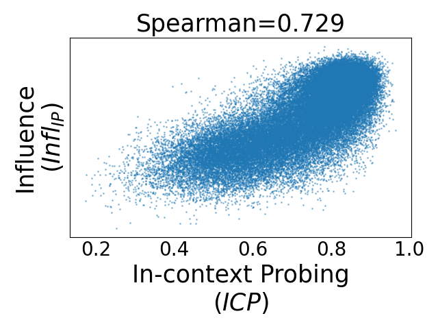
1a Spearman corr. ICP and $\text{Infl}_{\text{IF}}$.

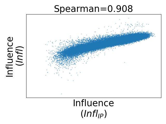
1b Spearman corr. Infl and $\text{Infl}_{\text{IP}}$.

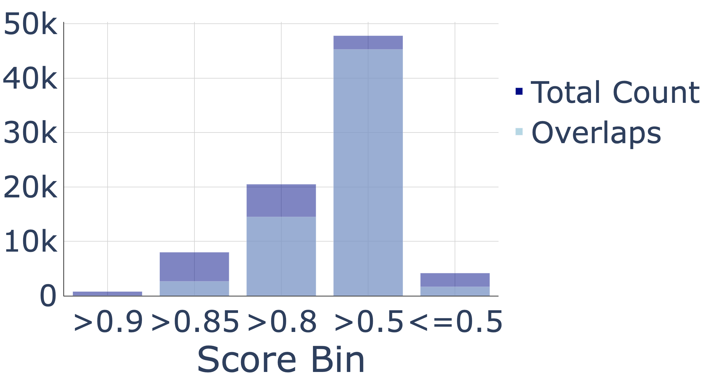
1c ICP and $\text{Infl}_{\text{IF}}$ ranking overlaps.

Figure 1: Correlation analysis between rankings on the instructions from the Alpaca dataset assigned by in-context probing and influence function approximations: $\text{Infl}_{\text{IF}}$ and Infl. Note: Infl was calculated with EK-FAC Grosse et al. (2023), as described in Section 6).

Table 1: Results (winrates) evaluated on the Alpaca Eval dataset after being finetuned on data selected by ICP and $\text{Infl}_{\text{IP}}$. The highest winrate in each column is marked with $*$ for ICP and $\dagger$ for $\text{Infl}_{\text{IP}}$.

Score Bin	Samples	Method	Helpful Base	Koala	Self Instruct	Oasst	Vicunna	Overall
$\leq 0.5$	$4186$	ICP	$47.65$	$58.17$	$59.2$	$55.61$	$61.25$	$56.51$
		$\text{Infl}_{\text{IP}}$	$49.21$	$57.79$	$56.97$	$59.89$	$54.43$	$56.31$
$>0.5$	$47816$	ICP	$57.03$	$\mathbf{71.61^{*}}$	$\mathbf{66.67^{*}}$	$56.99$	$61.53$	$64.75$
		$\text{Infl}_{\text{IP}}$	$54.33$	$54.33$	$\mathbf{66.67\dagger}$	$54.33$	$61.25$	$58.88$
$>0.8$	$20513$	ICP	$\mathbf{66.41^{*}}$	$69.07$	$62.15$	$\mathbf{67.57^{*}}$	$63.75$	$\mathbf{65.60^{*}}$
		$\text{Infl}_{\text{IP}}$	$53.9$	$\mathbf{70.39\dagger}$	$63.2$	$\mathbf{65.96\dagger}$	$67.5$	$\mathbf{64.17\dagger}$
$>0.85$	$8012$	ICP	$63.57$	$67.94$	$63.2$	$63.98$	$\mathbf{67.09^{*}}$	$64.75$
		$\text{Infl}_{\text{IP}}$	$\mathbf{61.42\dagger}$	$68.18$	$60.56$	$63.83$	$\mathbf{68.75\dagger}$	$63.75$
$>0.9$	$792$	ICP	$46.51$	$56.49$	$52.77$	$55.38$	$56.96$	$53.51$
		$\text{Infl}_{\text{IP}}$	$53.91$	$55.26$	$54.58$	$55.32$	$48.75$	$54.2$

We first compared the ranking of instructions scored by ICP and $\text{Infl}_{\text{IP}}$ on the Alpaca dataset. As shown in Figure 1a, the rankings are well-correlated (spearman=0.729, p<.05). Furthermore, Table 1 shows that fine-tuning on instruction data selected by ICP and $\text{Infl}_{\text{IP}}$ resulted in similar model performance among different score ranking bins. An exception can be observed in the Koala task in Table 1, where fine-tuning on data selected by ICP peaked the $>0.5$ score bin compared to $\text{Infl}_{\text{IP}}$ which peaked at the $>0.8$ score bin.

In addition, the overall performance for ICP and $\text{Infl}_{\text{IP}}$ both peaked at the $>0.8$ score bin, which followed the trend observed in Li et al. (2024b). Since Figure 1c also shows high overlap between instructions selected by both methods in the $>0.8$ score bin (overlap = $71\%$), this suggests that ICP and $\text{Infl}_{\text{IP}}$ have high agreement on instruction quality and valuation. Examples of top-ranked instructions selected by ICP and $\text{Infl}_{\text{IP}}$ are shown in Table D, and exhibit semantic similarities.

While our empirical results showed agreement between $\text{Infl}_{\text{IP}}$ for data valuation, a question can be raised on whether ICP and $\text{Infl}_{\text{IP}}$ both pick out inherently “good" training samples independently, or if they are actually connected through our theoretical analysis. In order to answer this question, we conducted experiments to empirically verify the middle steps of our theoretical analysis, which we describe in the following sections.

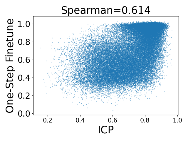
2a Spearman corr. between ICP and one-step finetune scores.

2b Spearman corr. between $\text{Infl}_{\text{IP}}$ and one-step finetune scores.

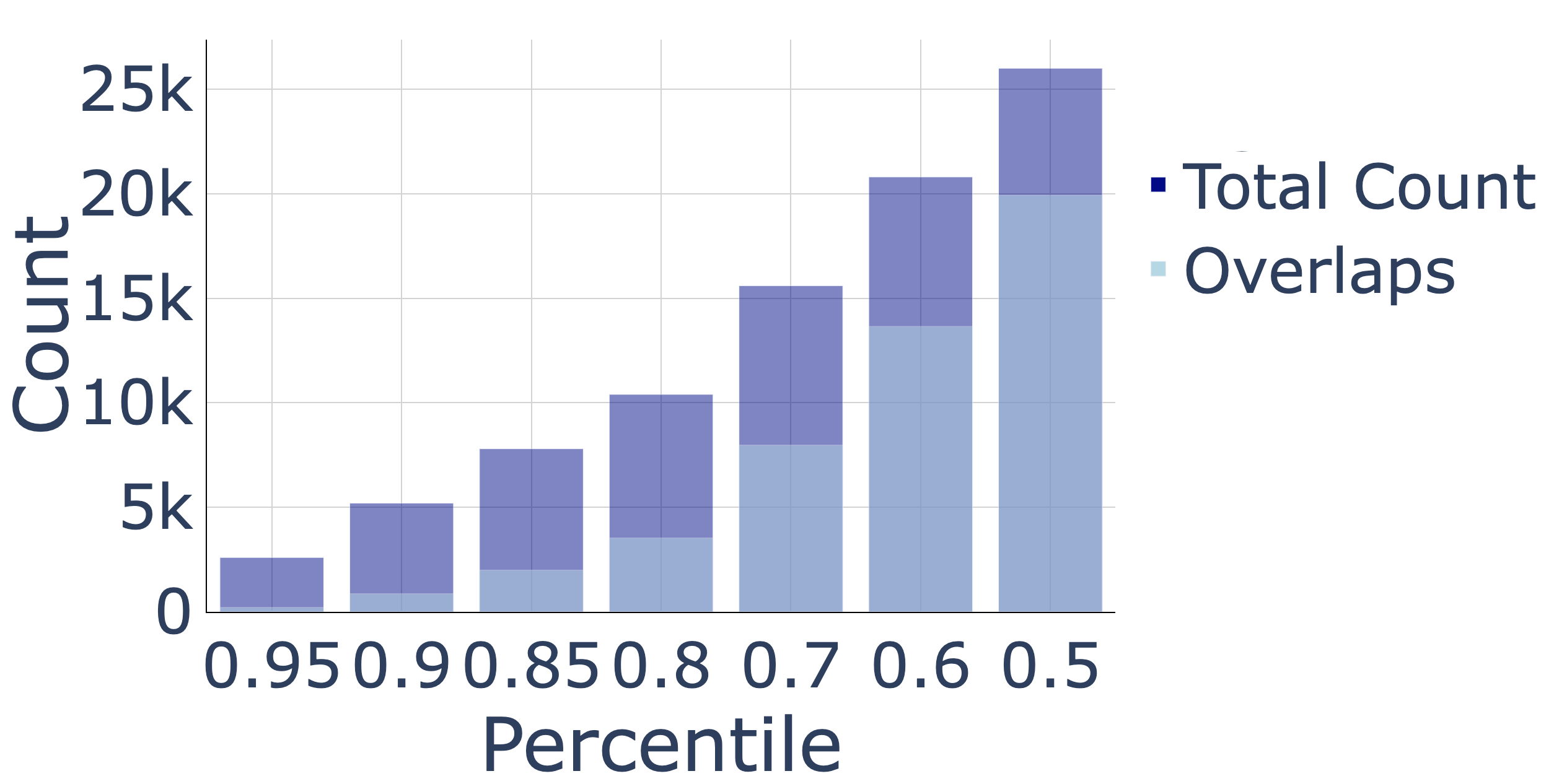
2c ICP and one-step finetune overlaps in score ranking percentiles.

Figure 2: Correlation analysis between rankings on the instructions from the Alpaca dataset assigned by in-context probing, $\text{Infl}_{\text{IP}}$, and one-step finetuning.

ICP vs. One-Step Fine-tuning: We first note that the key assumption in our analysis was: $s_{os}(x;z,\theta_{t})\approx s_{zs}(x;\theta_{t+1})$, which serves an important middle step between ICP and $\text{Infl}_{\text{IP}}$. To analyze this assumption empirically, we compared the ICP scores against a one-step fine-tune setup. In this setup, we took each instruction demonstration from the Alpaca Dataset and fine-tuned it for a single small step (lr=2e-5) on Pythia 1b-deduped. Each instruction demonstration was fine-tuned separately (i.e., no two instructions were fine-tuned on the same model), and model likelihoods where obtained for each example in the K-Means-100 dataset. Formally, for an instruction demonstration $z$ from the Alpaca Dataset, its one-step fine-tune score is:

$$\text{FT}(z,\mathcal{D})=\frac{1}{N}\sum_{i=1}^{N}\mathbbm{1}[s_{zs}(x_{i},\theta_{t+1})>s_{zs}(x_{i};\theta_{t})]$$

where $\theta_{t+1}=\theta_{t}-\eta_{t}\nabla\mathcal{L}(\theta_{t},z)$ denotes the parameters of the one-step fine-tuned model, and $\mathcal{D}$ denotes the K-Means-100 dataset for this setup.

We observed decent correlation (spearman=0.607, p<.05) and overlap between the ICP and one-step fine-tune score rankings as shown in figures 2a and 2c, respectively, which supports $s_{os}(x;z,\theta_{t})\approx s_{zs}(x;\theta_{t+1})$ in our setup.

Previous works have also shown that ICP and fine-tuning generate similar attention weights, and pay attention to similar training tokens Dai et al. (2023). However, these similarity scores have also been observed in models without in-context ability, Deutch et al. (2024), and may be weakened when considering order sensitivity Shen et al. (2024). Cases where the connection between ICP and one-step fine-tuning are strengthen or weakened can be left for future research.

One-Step Fine-tuning vs Influence: Given the empirical connection between ICP and one-step fine-tuning in the previous section, we also examined the empirical connection between one-step fine-tuning and $\text{Infl}_{\text{IP}}$ (i.e., $\text{Infl}_{\text{IP}}\approx s_{zs}(x;\theta_{t+1})-s_{zs}(x;\theta_{t})$) in order fully connect ICP to $\text{Infl}_{\text{IP}}$. We compared one-step fine-tuning scores from the previous section with the $\text{Infl}_{\text{IP}}$ scores on the Alpaca Dataset, and observed good correlation (spearman=0.772 p<.05) as shown in figure 2b. Given the theoretical and empirical ties from ICP to one-step fine-tuning to $\text{Infl}_{\text{IP}}$, our results suggests that ICP may serve as a proxy for $\text{Infl}_{\text{IP}}$ in this realm.

One observation from figures 2a and 2b to note is that some one-step fine-tune scores are top-heavy (i.e., closer to 1). There are a few possible explanations for this. For instance, performing a gradient descent step on a training sample involves updating model parameters as opposed to passing the training sample in-context. Consequently, the learning rate, optimization method, and model size are factors to take into account when performing one-step fine-tuning.

Hessian vs. Hessian-free Influence: Finally, we also compared data valuation ranking similarities between $\text{Infl}_{\text{IP}}$ and Infl. Following the same procedure as Section 5, we used $\text{Infl}_{\text{IP}}$ and Infl to rank training samples in the Alpaca dataset (Figure 1b), and observed strong correlation (spearman=0.91, p<.05) between the rankings. Note that for Infl, we use the EK-FAC Grosse et al. (2023) approximation for computing the inverse-Hessian product. Our results support previous works which suggested that dropping the Hessian can make $\text{Infl}_{\text{IP}}$ a suitable approximation for Infl Yang et al. (2024).

7 Conclusion

In this paper we provided both theoretical and empirical connections between in-context probing and influence functions. In turn, this offered a possible explanation for why in-context probing is effective for training data valuation. There are several lines of work that can further explore this phenomena. For instance, there may be stages of model training where the in-context probing is more beneficial than using influence functions for data selection, and vise versa. In addition, how these two data selection methods compare when selecting groups of training samples is another problem to consider.

8 Ethics and Limitations

First, we highlight limitations to our work. Our experiments were only conducted on Pythia-1b deduped. As model sizes change, the question of whether one data selection method triumphs over the other is an area for exploration. Furthermore, we note that we our experiments are in the realm of instruction-following tasks, and other types of tasks (e.g., question-answering, summarization) and training settings (e.g, pretraining) should be explored. We also note our evaluation metric (winrate) for instruction-following rely on LLM annotation, and may be subject to LLM bias as mentioned in Dubois et al. (2024a).

Since our work involves understanding data valuation in language models, we cannot foresee any immediate potential risks. However, we note that language models themselves can be susceptible to biases. We hope that this work can lead to future work in understanding the mechanisms of LLMs. Further insight in that realm may be beneficial in understanding model predictions, especially when considering LLM safety, toxicity, and biases.

Appendix

The appendix covers supporting information for our study. In Section A we provide a brief overview of influence functions. In Section B we discuss a framework introduced by Dai et al. (2023) which casts one-shot learning as implicit fine-tuning. In Section C we provide additional computations for the theoretical sketch we introduced in the paper. Finally, in Section D we show examples on top instructions selected by our different data valuation methods as noted in Section 5. We also provide a breakdown of the on the Alpaca Eval Dataset Li et al. (2023); Dubois et al. (2024b).

Appendix A Influence Functions

Given a dataset of training data $\mathcal{T}=\{z_{i}\}_{i}^{N}$, assume that model parameters $\theta$ fit the empirical risk minimization:

$$\theta^{*}=\operatorname*{arg\,min}_{\theta\in\mathbb{R}^{D}}\frac{1}{N}\sum_{i=1}^{N}\mathcal{L}(z_{i},\theta)$$ (9)

Now suppose we up-weight training example $z_{m}$ by a small value $\epsilon$. Then, the optimal solution to the empirical risk minimization becomes:

$$\theta^{*}(\epsilon)=\operatorname*{arg\,min}_{\theta\in\mathbb{R}^{D}}\frac{1}{N}\sum_{i=1}^{N}\mathcal{L}(z_{i},\theta)+\epsilon\mathcal{L}(z_{m},\theta)$$ (10)

Which is also called the response function. We wish to find the change in parameters $\Delta\theta=\theta^{*}(\epsilon)-\theta^{*}$, which can be done via a first-order Taylor approximation to the response function at $\epsilon=0$:

$$\theta^{*}(\epsilon)-\theta^{*}\approx\epsilon\dfrac{\operatorname{d\!}{}\theta^{*}(\epsilon)}{\operatorname{d\!}{\epsilon}}\bigg{\rvert}_{\epsilon=0}$$ (11)

Moreover, using the Implicit Function theorem, we get the influence of $z_{m}$ on $\theta^{*}$. ‹

$$I_{\theta^{*}}(z_{m})=\dfrac{\operatorname{d\!}{}\theta^{*}(\epsilon)}{\operatorname{d\!}{\epsilon}}\bigg{\rvert}_{\epsilon=0}=-H^{-1}\nabla_{\theta}\mathcal{L}(z_{m},\theta^{*})$$ (12)

where $H=\frac{1}{N}\sum_{i=1}^{N}\nabla_{\theta}^{2}\mathcal{L}(\theta^{*},\mathcal{T})$ is the Hessian. As mentioned in Grosse et al. (2023), since we often want to ground influence on something more concrete (e.g., a task), we can used a measurement $f(\theta)$, which results in:

$$I_{\theta^{*}}(z_{m})=-\nabla_{\theta}f(\theta^{*})^{T}H^{-1}\nabla_{\theta}\mathcal{L}(z_{m},\theta^{*})$$ (13)

For instance, if want measure how $z_{m}$ can increase a model’s likelihood probabilities on a test task $x=[x^{q};x^{a}]$, the we set $f(\theta)=\log p(x^{a}|x^{q};\theta)=-\mathcal{L}(\theta,x)$ and obtain:

$$I_{f}(z_{m})=\mathcal{L}(\theta,x)H^{-1}\nabla_{\theta}\mathcal{L}(z_{m},\theta^{*})$$ (14)

Appendix B One-Shot Learning as Implicit Fine-tuning

This section details the construction in Dai et al. (2023), which connects the transformer attention head to an implicit update step on the in-context demonstration. First, let $X_{train},X_{test}\in\mathbb{R}^{d}_{in}$ be the input representations of the train and test samples. Furthermore, we have the attention query vector $Q=W_{q}X^{T}_{test}$, the attention key vector $K=W_{k}[X_{train},X_{test}]$, and the attention value vector $V=W_{v}[X_{train},X_{test}]$ where $W_{k},W_{v},W_{q}\in\mathbb{R}^{d_{out}\times d_{in}}$. Then self-attention can be expressed as

$$Attention(K,V,Q) =W_{v}[X_{train},X_{test}]Softmax\left(\frac{W_{k}[X_{train},X_{test}]^{T}Q}{\sqrt{d_{in}}}\right)$$

$$\approx W_{v}[X_{train},X{x}]W_{k}[X_{train},X_{test}]^{T}Q$$

$$=W_{v}X_{test}(W_{k}X_{test})^{T}Q+W_{v}X_{train}(W_{k}X_{train})^{T}Q$$

$$=(W_{ZSL}+\Delta W_{ICL})Q$$ (15)

As seen above, the softmax is replaced with linear attention and the scaling factor $\sqrt{d_{in}}$ is removed. Furthermore, $W_{ZSL}$ is the zero-shot “attention head" weights and $\Delta W_{ICL}$ is the in-context demonstration update applied to $W_{ZSL}$.

Appendix C Proofs

Lemma 1.

Suppose we have a LLM with parameters $\theta_{t}$. At training iteration $t$, and we perform a stochastic gradient descent with training sample $z$ such that $\theta_{t+1}=\theta_{t}-\eta_{t}\nabla\mathcal{L}(\theta_{t},z)$. Then,

$$\text{Infl}_{\text{IP}}(z,x) =\nabla\mathcal{L}(\theta_{t},z)\cdot\nabla\mathcal{L}(\theta_{t},x)$$

$$\approx\frac{1}{\eta_{t}}\left(\mathcal{L}(x,\theta_{t})-\mathcal{L}(x,\theta_{t+1})\right)$$ (16)

Proof: This result above is discussed in Pruthi et al. (2020) and Iter et al. (2023). First, we consider the change in loss of $x$ using a first-order approximation:

$$\mathcal{L}(x,\theta_{t+1}) =\mathcal{L}(x,\theta_{t})+\nabla\mathcal{L}(\theta_{t},x)\dot{(}\theta_{t+1}-\theta_{t})+\mathcal{O}(||\theta_{t+1}-\theta_{t}||^{2})$$ (17)

Then, the change of loss is

$$\mathcal{L}(x,\theta_{t})-\mathcal{L}(x,\theta_{t+1}) =-\nabla\mathcal{L}(\theta_{t},x)\dot{(}\theta_{t+1}-\theta_{t})+\mathcal{O}(||\theta_{t+1}-\theta_{t}||^{2})$$

Next, suppose we take a stochastic gradient descent step on training sample $z$. Then, the model parameters are updated as: $\theta_{t+1}=\theta_{t}-\eta_{t}\nabla\mathcal{L}(\theta_{t},z)$. Thus, we have $\theta_{t+1}-\theta_{t}=-\eta_{t}\nabla\mathcal{L}(\theta_{t},z)$. Then, the above equation can be written as

$$\mathcal{L}(x,\theta_{t})-\mathcal{L}(x,\theta_{t+1}) \approx\eta_{t}\nabla\mathcal{L}(\theta_{t},x)\cdot\nabla\mathcal{L}(\theta_{t},z)$$ (19)

Given that $\eta_{t}$ is small (and thus $||\theta_{t+1}-\theta_{t}||^{2}$ is small).

Lemma 2.

Let $\mathcal{L}(x,\theta)$ be the conditional cross-entropy loss for a task $x=[x^{q};x^{a}]$. Then,

$$\mathcal{L}(x,\theta)=-s_{zs}(x,\theta_{t})$$

Proof:

$$\mathcal{L}(x,\theta) =-\frac{1}{L}\sum_{j=1}^{L}\log p_{\theta}(x_{i,j}^{a}|x_{i}^{q},x_{i,<j-1}^{a})$$

$$=-s_{zs}(x,\theta)$$

Appendix D Additional Tables and Figures

$ICP$	$\text{Infl}_{\text{IP}}$
⬇ Instruction: Create an array containing the first 10 prime numbers. ⬇ Response: Here is an array containing the first 10 prime numbers: [2, 3, 5, 7, 11, 13, 17, 19, 23, 29]	⬇ Instruction: Create an array containing the first 10 prime numbers. ⬇ Response: Here is an array containing the first 10 prime numbers: [2, 3, 5, 7, 11, 13, 17, 19, 23, 29]
⬇ Instruction: Write an algorithm for printing all prime numbers between 0 and 100. ⬇ Response: Here is an algorithm for printing all prime numbers between 0 and 100: 1. Start with a variable ‘n‘ at 2, since 2 is the first prime number. 2. Create a loop that will iterate until ‘n‘ is greater than 100. 3. At each iteration of the loop, check if ‘n‘ is prime ...	⬇ Instruction: Given an array of integers and a target number, find a triplet which adds up to the target number. Input: Array: [2, 5, 3, 6, 9], Target: 12 ⬇ Response: One possible solution is to sort the array and then use two pointers to check for possible triplets. Here is the step-by-step process: 1. Sort the array in ascending order. In this case, it will be [2, 3, 5, 6, 9]. 2. Initialize a pointer ‘i‘ to the first element ...
⬇ Instruction: Generate a random string of 5 lowercase letters. ⬇ Response: Here is a randomly generated string of 5 lowercase letters: "kdjyr"	⬇ Instruction: Create an algorithm to sort a given array of numbers. Input: [7, 1, 3, 5, 9] ⬇ Response: There are many algorithms to sort a given array of numbers. Below is one such algorithm using the Bubble Sort method: 1. Begin by comparing the first two elements of the array ...
⬇ Instruction: Generate a random password with 8 characters, consisting of lower and upper-case letters and numbers. ⬇ Response: Here is a randomly generated password with 8 characters, consisting of lower and upper-case letters and numbers: "aB3dE6fG"	⬇ Instruction: Create an algorithm in pseudocode that sorts an array of numbers using the selection sort method. Input: Array: [3, 1, 4, 7, 8, 2] ⬇ Response: Here is a pseudocode that sorts an array of numbers using the selection sort method: Procedure selection_sort(Array: list of sortable items) BEGIN Declare index_min, temporary ...
⬇ Instruction: Create an algorithm to find the maximum value in an array of numbers. Input: [3, 5, 7, 2] ⬇ Response: Here is an algorithm to find the maximum value in an array of numbers: 1. Initialize the first element of the array as the maximum value. 2. Loop through the rest of the array, comparing each element with the current maximum value. 3. If the current element is ...	⬇ Instruction: Create a PHP script to detect whether a string contains a number. ⬇ Response: Here is one way to create a PHP script to detect whether a string contains a number: ‘‘‘ <?php function containsNumber($str) { // check if the input string contains any digits if (preg_match(’/\d/’, $str)) { return true; } else { return false; } } // test ...

Table 2: The top-5 demonstrations selected by ICP and $\text{Infl}_{\text{IP}}$ for the test task: Instruction: Create an array containing the first 10 prime numbers.

Subset	Number of Examples
Helpful Base Bai et al. (2022)	129
Koala Geng et al. (2023)	156
Self-Instruct Wang et al. (2023)	252
Oasst	188
Vicuna Chiang et al. (2023)	80

Table 3: Breakdown of the subsets in the Alpaca Eval Li et al. (2023); Dubois et al. (2024b) dataset.

References

- Albalak et al. (2024) Alon Albalak, Yanai Elazar, Sang Michael Xie, Shayne Longpre, Nathan Lambert, Xinyi Wang, Niklas Muennighoff, Bairu Hou, Liangming Pan, Haewon Jeong, Colin Raffel, Shiyu Chang, Tatsunori Hashimoto, and William Yang Wang. 2024. A survey on data selection for language models. Preprint, arXiv:2402.16827.
- Bai et al. (2022) Yuntao Bai, Andy Jones, Kamal Ndousse, Amanda Askell, Anna Chen, Nova DasSarma, Dawn Drain, Stanislav Fort, Deep Ganguli, Tom Henighan, Nicholas Joseph, Saurav Kadavath, Jackson Kernion, Tom Conerly, Sheer El-Showk, Nelson Elhage, Zac Hatfield-Dodds, Danny Hernandez, Tristan Hume, Scott Johnston, Shauna Kravec, Liane Lovitt, Neel Nanda, Catherine Olsson, Dario Amodei, Tom Brown, Jack Clark, Sam McCandlish, Chris Olah, Ben Mann, and Jared Kaplan. 2022. Training a helpful and harmless assistant with reinforcement learning from human feedback. Preprint, arXiv:2204.05862.
- Basu et al. (2021) Samyadeep Basu, Philip Pope, and Soheil Feizi. 2021. Influence functions in deep learning are fragile. Preprint, arXiv:2006.14651.
- Biderman et al. (2023) Stella Biderman, Hailey Schoelkopf, Quentin Anthony, Herbie Bradley, Kyle O’Brien, Eric Hallahan, Mohammad Aflah Khan, Shivanshu Purohit, USVSN Sai Prashanth, Edward Raff, Aviya Skowron, Lintang Sutawika, and Oskar van der Wal. 2023. Pythia: A suite for analyzing large language models across training and scaling. Preprint, arXiv:2304.01373.
- Chen et al. (2024) Lichang Chen, Shiyang Li, Jun Yan, Hai Wang, Kalpa Gunaratna, Vikas Yadav, Zheng Tang, Vijay Srinivasan, Tianyi Zhou, Heng Huang, and Hongxia Jin. 2024. Alpagasus: Training a better alpaca with fewer data. Preprint, arXiv:2307.08701.
- Chiang et al. (2023) Wei-Lin Chiang, Zhuohan Li, Zi Lin, Ying Sheng, Zhanghao Wu, Hao Zhang, Lianmin Zheng, Siyuan Zhuang, Yonghao Zhuang, Joseph E Gonzalez, et al. 2023. Vicuna: An open-source chatbot impressing gpt-4 with 90%* chatgpt quality. See https://vicuna. lmsys. org (accessed 14 April 2023), 2(3):6.
- Dai et al. (2023) Damai Dai, Yutao Sun, Li Dong, Yaru Hao, Shuming Ma, Zhifang Sui, and Furu Wei. 2023. Why can GPT learn in-context? language models secretly perform gradient descent as meta-optimizers. In Findings of the Association for Computational Linguistics: ACL 2023, pages 4005–4019, Toronto, Canada. Association for Computational Linguistics.
- Deutch et al. (2024) Gilad Deutch, Nadav Magar, Tomer Bar Natan, and Guy Dar. 2024. In-context learning and gradient descent revisited. Preprint, arXiv:2311.07772.
- Dubois et al. (2024a) Yann Dubois, Balázs Galambosi, Percy Liang, and Tatsunori B. Hashimoto. 2024a. Length-controlled alpacaeval: A simple way to debias automatic evaluators. Preprint, arXiv:2404.04475.
- Dubois et al. (2024b) Yann Dubois, Xuechen Li, Rohan Taori, Tianyi Zhang, Ishaan Gulrajani, Jimmy Ba, Carlos Guestrin, Percy Liang, and Tatsunori B. Hashimoto. 2024b. Alpacafarm: A simulation framework for methods that learn from human feedback. Preprint, arXiv:2305.14387.
- Engstrom et al. (2024) Logan Engstrom, Axel Feldmann, and Aleksander Madry. 2024. Dsdm: Model-aware dataset selection with datamodels. arXiv preprint arXiv:2401.12926.
- Geng et al. (2023) Xinyang Geng, Arnav Gudibande, Hao Liu, Eric Wallace, Pieter Abbeel, Sergey Levine, and Dawn Song. 2023. Koala: A dialogue model for academic research.
- Goyal et al. (2024) Sachin Goyal, Pratyush Maini, Zachary C. Lipton, Aditi Raghunathan, and J. Zico Kolter. 2024. Scaling laws for data filtering – data curation cannot be compute agnostic. Preprint, arXiv:2404.07177.
- Grosse et al. (2023) Roger Grosse, Juhan Bae, Cem Anil, Nelson Elhage, Alex Tamkin, Amirhossein Tajdini, Benoit Steiner, Dustin Li, Esin Durmus, Ethan Perez, Evan Hubinger, Kamilė Lukošiūtė, Karina Nguyen, Nicholas Joseph, Sam McCandlish, Jared Kaplan, and Samuel R. Bowman. 2023. Studying large language model generalization with influence functions. Preprint, arXiv:2308.03296.
- Han et al. (2023) Xiaochuang Han, Daniel Simig, Todor Mihaylov, Yulia Tsvetkov, Asli Celikyilmaz, and Tianlu Wang. 2023. Understanding in-context learning via supportive pretraining data. In Proceedings of the 61st Annual Meeting of the Association for Computational Linguistics (Volume 1: Long Papers), pages 12660–12673, Toronto, Canada. Association for Computational Linguistics.
- Iter et al. (2023) Dan Iter, Reid Pryzant, Ruochen Xu, Shuohang Wang, Yang Liu, Yichong Xu, and Chenguang Zhu. 2023. In-context demonstration selection with cross entropy difference. In Findings of the Association for Computational Linguistics: EMNLP 2023, pages 1150–1162, Singapore. Association for Computational Linguistics.
- Koh and Liang (2017) Pang Wei Koh and Percy Liang. 2017. Understanding black-box predictions via influence functions. In International conference on machine learning, pages 1885–1894. PMLR.
- Lee et al. (2022) Katherine Lee, Daphne Ippolito, Andrew Nystrom, Chiyuan Zhang, Douglas Eck, Chris Callison-Burch, and Nicholas Carlini. 2022. Deduplicating training data makes language models better. Preprint, arXiv:2107.06499.
- Li et al. (2024a) Ming Li, Yong Zhang, Zhitao Li, Jiuhai Chen, Lichang Chen, Ning Cheng, Jianzong Wang, Tianyi Zhou, and Jing Xiao. 2024a. From quantity to quality: Boosting llm performance with self-guided data selection for instruction tuning. Preprint, arXiv:2308.12032.
- Li et al. (2023) Xuechen Li, Tianyi Zhang, Yann Dubois, Rohan Taori, Ishaan Gulrajani, Carlos Guestrin, Percy Liang, and Tatsunori B Hashimoto. 2023. Alpacaeval: An automatic evaluator of instruction-following models.
- Li et al. (2024b) Yunshui Li, Binyuan Hui, Xiaobo Xia, Jiaxi Yang, Min Yang, Lei Zhang, Shuzheng Si, Junhao Liu, Tongliang Liu, Fei Huang, and Yongbin Li. 2024b. One shot learning as instruction data prospector for large language models. Preprint, arXiv:2312.10302.
- Nguyen and Wong (2023) Tai Nguyen and Eric Wong. 2023. In-context example selection with influences. Preprint, arXiv:2302.11042.
- Olsson et al. (2022) Catherine Olsson, Nelson Elhage, Neel Nanda, Nicholas Joseph, Nova DasSarma, Tom Henighan, Ben Mann, Amanda Askell, Yuntao Bai, Anna Chen, et al. 2022. In-context learning and induction heads. arXiv preprint arXiv:2209.11895.
- Park et al. (2023) Sung Min Park, Kristian Georgiev, Andrew Ilyas, Guillaume Leclerc, and Aleksander Mądry. 2023. Trak: attributing model behavior at scale. In Proceedings of the 40th International Conference on Machine Learning, ICML’23. JMLR.org.
- Pruthi et al. (2020) Garima Pruthi, Frederick Liu, Mukund Sundararajan, and Satyen Kale. 2020. Estimating training data influence by tracing gradient descent. Preprint, arXiv:2002.08484.
- Rubin et al. (2022) Ohad Rubin, Jonathan Herzig, and Jonathan Berant. 2022. Learning to retrieve prompts for in-context learning. Preprint, arXiv:2112.08633.
- Shen et al. (2024) Lingfeng Shen, Aayush Mishra, and Daniel Khashabi. 2024. Do pretrained transformers learn in-context by gradient descent? Preprint, arXiv:2310.08540.
- Sorscher et al. (2023) Ben Sorscher, Robert Geirhos, Shashank Shekhar, Surya Ganguli, and Ari S. Morcos. 2023. Beyond neural scaling laws: beating power law scaling via data pruning. Preprint, arXiv:2206.14486.
- Taori et al. (2023) Rohan Taori, Ishaan Gulrajani, Tianyi Zhang, Yann Dubois, Xuechen Li, Carlos Guestrin, Percy Liang, and Tatsunori B Hashimoto. 2023. Stanford alpaca: An instruction-following llama model.
- Von Oswald et al. (2023) Johannes Von Oswald, Eyvind Niklasson, Ettore Randazzo, João Sacramento, Alexander Mordvintsev, Andrey Zhmoginov, and Max Vladymyrov. 2023. Transformers learn in-context by gradient descent. In International Conference on Machine Learning, pages 35151–35174. PMLR.
- Wang et al. (2023) Yizhong Wang, Yeganeh Kordi, Swaroop Mishra, Alisa Liu, Noah A. Smith, Daniel Khashabi, and Hannaneh Hajishirzi. 2023. Self-instruct: Aligning language models with self-generated instructions. In Proceedings of the 61st Annual Meeting of the Association for Computational Linguistics (Volume 1: Long Papers), pages 13484–13508, Toronto, Canada. Association for Computational Linguistics.
- Wettig et al. (2024) Alexander Wettig, Aatmik Gupta, Saumya Malik, and Danqi Chen. 2024. Qurating: Selecting high-quality data for training language models. arXiv preprint arXiv:2402.09739.
- Xia et al. (2024) Mengzhou Xia, Sadhika Malladi, Suchin Gururangan, Sanjeev Arora, and Danqi Chen. 2024. Less: Selecting influential data for targeted instruction tuning. Preprint, arXiv:2402.04333.
- Xie et al. (2023) Sang Michael Xie, Hieu Pham, Xuanyi Dong, Nan Du, Hanxiao Liu, Yifeng Lu, Percy Liang, Quoc V. Le, Tengyu Ma, and Adams Wei Yu. 2023. Doremi: Optimizing data mixtures speeds up language model pretraining. Preprint, arXiv:2305.10429.
- Xie et al. (2021) Sang Michael Xie, Aditi Raghunathan, Percy Liang, and Tengyu Ma. 2021. An explanation of in-context learning as implicit bayesian inference. arXiv preprint arXiv:2111.02080.
- Yang et al. (2024) Ziao Yang, Han Yue, Jian Chen, and Hongfu Liu. 2024. Revisit, extend, and enhance hessian-free influence functions. Preprint, arXiv:2405.17490.
- Ye et al. (2024) Jiasheng Ye, Peiju Liu, Tianxiang Sun, Yunhua Zhou, Jun Zhan, and Xipeng Qiu. 2024. Data mixing laws: Optimizing data mixtures by predicting language modeling performance. Preprint, arXiv:2403.16952.