COKE: Causal Discovery with Chronological Order and Expert Knowledge in High Proportion of Missing Manufacturing Data

Abstract.

Understanding causal relationships between machines is crucial for fault diagnosis and optimization in manufacturing processes. Real-world datasets frequently exhibit up to 90% missing data and high dimensionality from hundreds of sensors. These datasets also include domain-specific expert knowledge and chronological order information, reflecting the recording order across different machines, which is pivotal for discerning causal relationships within the manufacturing data. However, previous methods for handling missing data in scenarios akin to real-world conditions have not been able to effectively utilize expert knowledge. Conversely, prior methods that can incorporate expert knowledge struggle with datasets that exhibit missing values. Therefore, we propose COKE to construct causal graphs in manufacturing datasets by leveraging expert knowledge and chronological order among sensors without imputing missing data. Utilizing the characteristics of the recipe, we maximize the use of samples with missing values, derive embeddings from intersections with an initial graph that incorporates expert knowledge and chronological order, and create a sensor ordering graph. The graph-generating process has been optimized by an actor-critic architecture to obtain a final graph that has a maximum reward. Experimental evaluations in diverse settings of sensor quantities and missing proportions demonstrate that our approach compared with the benchmark methods shows an average improvement of 39.9% in the F1-score. Moreover, the F1-score improvement can reach 62.6% when considering the configuration similar to real-world datasets, and 85.0% in real-world semiconductor datasets. The source code is available at https://github.com/OuTingYun/COKE.

1. Introduction

Figure 1. Manufacturing process workflow. Products sequentially interact with sensors across various machines, with an established order that ensures each sensor influences only subsequent sensors on the same or next machines.

The manufacturing industry is increasingly transitioning towards automation and complexity to enhance product quality and variety (Liang et al., 2004; Colledani et al., 2014). For instance, semiconductor (Yang et al., 2023a) and fluid catalytic cracking processes (Gharahbagheri et al., 2015) involve hundreds of machines. This complexity poses challenges in understanding the underlying causal mechanisms of production lines and identifying the root causes of system failures and product defects. In this scenario, understanding the causal relationships between machines is crucial. It enhances engineers’ understanding of the system and enables the tracking of the root causes of failure events, thereby facilitating real-time error correction even in the absence of on-site engineers (Ezukwoke et al., 2024; Ikram et al., 2022; Qin et al., 2022). Furthermore, understanding the causal relationships between components can offer preemptive alerts for prospective errors to reduce assembly line downtime (Huegle et al., 2020; Hagedorn et al., 2022). Therefore, employing causal discovery methods in manufacturing data is important in the recent evolution of manufacturing (Marazopoulou et al., 2016).

In the manufacturing process, the datasets include domain-specific expert knowledge to modify or retain certain edges and chronological order capturing the sequence of data recordings across various machines. The expert knowledge and chronological order reflect true interactions and dependencies influenced by the manufacturing process (Marazopoulou et al., 2016). Expert knowledge distinguishes between causal relationships from mere correlations, while chronological data captures the sequence of events, aiding in identifying how changes or errors propagate through the system. Therefore, it is essential to leverage information when accurately identifying causal relationships within the manufacturing data. Recent research (Yang et al., 2023b) inspired by Bühlmann et al. (2013), divided causal discovery into two stages: ordering graph generation and neighbor variables selection. This approach allows the design of a model that can utilize a prior knowledge graph for constructing the causal graph. However, in manufacturing data, the recipes result in datasets with a high proportion of missing values, as shown in Figure 1. The recipes determine which machines and sensors are involved in the production process, and the sequence of machines used in it. The variability in recipes across different product configurations can lead to the occurrence of missing values in the dataset (Kwak and Kim, 2012). For example, consider a manufacturing facility that produces semiconductors with varying specifications. Certain product configurations may bypass certain machines or sensors, resulting in missing data for those particular sensors (Yang et al., 2023a). As a result, the dataset may exhibit a high missing rate, particularly for sensors associated with less frequently used product configurations. Consequently, before applying a method (Yang et al., 2023b) that could effectively leverage expert knowledge and chronological order in manufacturing data, it is essential to impute missing data, potentially compromising the optimal efficacy of the solution.

With missing rates in manufacturing data reaching up to 90%, imputed data significantly impact the dataset’s distribution and affect the performance of results. To avoid bias from imputed data, some previous approaches will pre-define the types of missing data. According to (Rubin, 1976), based on the different types of missingness, the underlying missing mechanism can be divided into three basic types: missing at random (MAR), missing completely at random (MCAR), and missing not at random (MNAR). However, the missingness in manufacturing data stems from variations in recipes, leading to unsuitable accurate definitions of the types of missing data. This obstacle complicates the selection of appropriate methods for causal discovery and the optimization of their utilization in data processing. Other methods that do not specify missing data types struggle with incorporating expert knowledge and chronological order information among sensors (Morales-Alvarez et al., 2022; Tu et al., 2018), and are inefficient in processing datasets with hundreds of variables (Gao et al., 2022).

When constructing a causal graph from manufacturing data, expert knowledge and chronological order information are crucial as they impact the causal relationships between sensors. However, existing methods struggle to address the challenge posed by high proportions of missing values in data with varied recipes. Additionally, methods capable of handling missing data fail to effectively leverage expert knowledge and chronological order information. To address these challenges, we propose COKE, which leverages Chronological Order and expert KnowledgE using a graph attention network. This approach optimizes the utilization of samples with missing values by recipes in manufacturing data, thereby avoiding the need for data imputation and achieving accurate variable embeddings. Upon obtaining embeddings for each variable (sensor), we use a decoder to sequence the variables by causal order. We then remove edges from the ordering graph based on these sequenced variables using the initial graph. We employ an actor-critic architecture to optimize our graph generation model, aiming to maximize the reward by minimizing the Bayesian Information Criterion (BIC) score. Throughout the training, we record the graph in each iteration, ultimately selecting the graph with the highest reward as the final causal graph for the manufacturing dataset.

Our contributions can be summarized as follows: 1) We introduce COKE, a novel deep learning approach designed to address the challenge of effectively utilizing expert knowledge and chronological order in datasets with up to 90% of missing values. 2) We utilize recipes in the manufacturing process to generate embeddings that comprehensively represent variables without imputing missing values. 3) In the scenarios involving diverse quantities and missing rates on synthetic data simulating the real-world dataset distributions, our approach demonstrates enhancing the F1-score by 39.9% compared to the benchmark. Additionally, on real-world data, it achieves an improvement above 85.0%. Furthermore, through ablation studies, we demonstrate the impact of expert knowledge and chronological order in the graph-constructing process from manufacturing data.

2. Related Work

2.1. Causal Discovery with Incomplete Data

Causal graph construction in the presence of missing data requires considering the impact of missing values on causal discovery. Tu et al. (2018) extended the constraint-based PC algorithm by analyzing observed data to identify potential errors or inconsistencies in causal relationships between variables. They also proposed corrective measures to achieve a more accurate representation of the true causal graph. Qiao et al. (2024) utilized additive noise models, expanding the identifiability results of causal discovery methods, including the recognition of causal skeletons and weakly self-concealing missingness. However, these constraint-based methods based on the PC algorithm result in ineffectively constructing graphs for data with hundreds of variables because of the exponential growth of conditional sets (Le et al., 2019). MissDAG (Gao et al., 2022) employs the Monte Carlo EM framework. In the E-step, the model estimates the data distribution from the observed available data, taking into account the missing values. The M-step then utilizes the causal discovery model to estimate the data and identify the causal graph among variables. However, this method is time-consuming for hundreds of variables and cannot utilize expert knowledge and chronological order in the graph-constructing process. Several methods use machine learning techniques to address the missing values in the dataset. (Morales-Alvarez et al., 2022; Wang et al., 2020; Gao and Cai, 2023; Huang et al., 2020) obtained the precise characteristics of data distributions, enabling the identification of causal relationships by uncovering the correct distribution from the data. These methods perform end-to-end training on generative adversarial network-based imputation models and causal structure learning models. However, they are unsuitable for manufacturing datasets since they do not account for expert knowledge and chronological order.

2.2. Causal Discovery in Manufacturing Data

Advancements in manufacturing processes, automated measurement tools, and real-time data collection have improved data quality, facilitating accurate representation of product conditions (Clavijo et al., 2021). As a result, there has been significant progress in applying causal discovery techniques within the manufacturing data. Yang et al. (2023a) proposed a causal structure learning method for wafer manufacturing data, which utilizes a hierarchical structure to decompose complex causal discovery into smaller substructures. It integrates learning multiple causal discovery algorithms to improve the robustness and accuracy of the learned structure. However, this work assumes that sensors on the same machine lack causal relationships, thereby limiting its ability to accurately identify the causal-effect relationships between sensors within the same machine. Marazopoulou et al. (2016) applied data mining and knowledge discovery to root cause analysis in the manufacturing and interconnected industries, while (Abu-Samah et al., 2015) constructs a causal graph taking the minimum description length (MDL) constructed the scoring function, followed by subsequent root cause analysis and application to process reactors. However, these methods only consider a few machines in the dataset, as does the work in multi-stage PCB manufacturing (Sim et al., 2014). While there are many methods for constructing causal graphs from manufacturing data, they face challenges with datasets in high proportions of missing values or limited dimensions, affecting improper application for our problem.

Despite the high proportion of missing values in the dataset, we can obtain complete datasets through imputation for causal discovery. Notears (Zheng et al., 2018), a widely-used method, reformulates causal discovery as a continuous function optimization problem from a combination problem. This method inspired (Bühlmann et al., 2013; Wang et al., 2021; Yang et al., 2023b; Morales-Alvarez et al., 2022) to integrate machine learning techniques for causal discovery problems. ICA-LiNGAM (Shimizu et al., 2006) addresses linear non-Gaussian models with continuous-valued data, while GARL(Yang et al., 2023b) trains the graph-generating process by optimizing the score function using an actor-critic architecture. However, imputation bias with up to 90% missing values leads to inaccurate results of causal discovery.

3. Preliminary

3.1. Problem Formulation

In the manufacturing dataset, the recorded process follows the description in Figure 1. The dataset is represented as $D=(X,d,k,\Gamma)$, where $X=[X_{1},\dots,X_{d}]^{T}\in\mathbb{R}^{N\times d}$, with $N$ samples and $d$ sensors. $k$ denotes the number of machines and $k_{d}$ means the corresponding machine for sensor $d$. In the graph generated from observational data, each variable $x_{i}$ corresponds to sensor $i$ in the manufacturing process. $\Gamma=\{r_{1},\ldots,r_{s}\}$ represents a set of $s$ recipes within $X$, where each $r_{i}$ comprises a different number of samples denoted as $n_{i}$, resulting in a total of $N=\sum_{i=1}^{s}n_{i}$. Then we can partition the dataset into $X=[X^{r_{1}},\ldots,X^{r_{s}}]$ and each $X^{r_{i}}\in\mathbb{R}^{n_{i}\times d}$ contains $d$ variables. The dataset $X$ is divided by recipes into subsets $X^{r_{i}}$, each containing observed data $X^{r_{i}}_{o(r_{i})}$ and missing data $X^{r_{i}}_{m(r_{i})}$. Here, $m(r_{i})$ denotes the set of variables (sensors) that are missing due to bypass in the recipe $r_{i}$, while $o(r_{i})$ represents the set of variables that are observed. As shown in Figure 1, $o(r_{3})$ is $\{x_{1},x_{2},\dots\}$, and $X^{r_{3}}_{o(r_{3})}$ denotes a complete dataset in $r_{3}$. We also define the specific recipe as $r_{full}$ where $|o(r_{full})|=d$ and the corresponding subset $X^{r_{full}}$ is completed. Hence, there are $(s-1)$ subsets that are incomplete, denoted as $X^{r_{miss}}=\{X^{r_{i}}\>|\>r_{i}\in\Gamma\>\text{and}\>|o(r_{i})|<d\}$. Example of $X^{r_{full}}$ and $X^{r_{miss}}$ are shown in Figure 1.

3.2. Model Definition

In this work, we represent the causal graph as ${G}=({V,E})$ , where $V=\{1,...,d\}$ is a set containing $d$ variables, and $E=\{(i,j)\>|\>i,j=1,\ldots d\}$ is a set of directed edges from variable $i$ to variable $j$. Each variable in the causal graph is denoted as $x_{i}$, where $i\in V$. The assumption of the data generation process is followed by

$$\small x_{i}=f_{i}(x_{Pa(i)})+\eta_{i},\>i=1,\ldots,d,$$

where $x_{Pa(i)}=\{k\>|\>(k,i)\in E\}$ is the set of parent variables for $x_{i}$, and $f_{i}(\cdot)$ represents the causal relationship between $x_{i}$ and $x_{Pa(i)}$. We follow the assumption of (Wang et al., 2021) that assumes the noise $\eta_{i}\sim\mathcal{N}(0,\sigma^{2})$ is jointly independent with variables in ${x_{Pa(i)}}$ and the causal minimality for each function $f_{i}(\cdot)$ is not constant. Additionally, we assume that all variables are measurable (causally sufficient) and there are no confounders, which are latent causes of the observed variables in the dataset. Given the observational data $X={[X_{1},..X_{d}]}^{T}\in\mathbb{R}^{N\times d}$ the goal of causal discovery is to find hidden cause-effect relationships between variables from the observational data.

3.3. Ordering Variable Definition

In previous work, the task of identifying a direct acyclic graph can be defined as determining a variable ordering (Bühlmann et al., 2013; Wang et al., 2021; Teyssier and Koller, 2005). Let $\Pi$ be a set of ordering variable (sensors) for $V$ and $|\Pi|=d$, if the $q$-th variable in $\Pi$ is $x_{i}$ then $\Pi(q)=x_{i}$. We denote a direct acyclic graph (DAG) as $\mathcal{G}$. For any ordering variable set $\Pi$, we can construct a DAG $\mathcal{G}^{\Pi}$ which has directed edges from $\Pi(i)$ to $\Pi(j)$ for any $i<j$, as shown in Figure 4. A $\mathcal{G}$ can consist of more than one ordering variable set, denoted as:

$$\small\Phi(\mathcal{G})=\{\Pi:\mathcal{G}^{\Pi}\>\text{is a super-DAG of}\>\>\mathcal{G}\},$$

where a super-DAG of $\mathcal{G}$ is a DAG whose edge set is a superset of $\mathcal{G}$. To find true DAG $\mathcal{G}^{*}$, Bühlmann et al. (2013) separated the causal discovery problem to find the ordering variable sets of the true DAG $\Phi(\mathcal{G^{*}})$ and variables selection in each $\Pi\in\Phi(\mathcal{G^{*}})$. We constructed an initial graph $g_{init}$ with $d$ variables to assist the variables selection in each ordering variable set in $\Phi(\mathcal{G^{*}})$. To ensure comprehensive consideration of information between variables, the graph contains all potential causal relationships; thus, all variables are fully connected in the initial graph $g_{init}$.

4. Method

Figure 2. The overview framework of COKE. In this framework: 1) the actor obtains a causal graph from the ordering graph, which is generated by the dataset and the initial graph with expert knowledge and chronological order information; 2) the reward function evaluates the graph produced by the actor using the complete dataset; 3) the critic network assesses the current state’s value, guiding the actor network’s update through gradients derived from the reward and value.

In our task, we aim to derive the true DAG $\mathcal{G}^{*}$ from the observed dataset $X$, which contains a high proportion of missing values. To address this challenge, we break down the causal discovery task into two main components: ordering graph generation and variables selection. Firstly, in Section 4.1, we modify an initial graph by incorporating expert knowledge and chronological ordering. In Section 4.2, we generate the ordering without imputation by leveraging the characteristics of recipes in the manufacturing dataset and utilizing the initial graph. Then, in Section 4.3, we determine the ordering variable $\Pi^{*}$ that maximizes the reward function through variables selection based on the initial graph. The framework of our proposed method is illustrated in Figure 2.

4.1. Initial Graph Construction with Expert Knowledge and Chronological Order

In manufacturing data, since products pass through machines sequentially, chronological order occurs between the machines. Therefore, we reduce the space of $\Phi(\mathcal{G^{*}})$ by permuting the machines in the manufacturing data:

(1) $$\small\bar{\Phi}(\mathcal{G^{*}})=\{\Pi\>|\>for\>i<j,\>\>k_{\Pi(i)}\leq k_{\Pi(j)}\}\subset\Phi(\mathcal{G^{*}}),$$

where $k_{\Pi(i)}$ represents the corresponding machine of sensor ${\Pi(i)}$. For true DAG, $\bar{\Phi}(\mathcal{G^{*}})$ contains ordering variable sets that conform to chronological order information. We refine the initial graph $g_{init}$ by removing the edges that are not in the union of all $\Pi\in\bar{\Phi}(\mathcal{G^{*}})$. Then, we define $g_{k}$ as the initial graph that accounts for the chronological order among machines. We apply preliminary neighbor selection (PNS) to the initial graph $g_{k}$ by the assumption that the result of PNS on $g_{k}$ contains all correct edges (Bühlmann et al., 2013). Subsequently, we modify the edges based on expert knowledge by removing or adding them accordingly. Therefore, the initial graph $g_{k}$ includes expert knowledge and chronological order information, making it ready for ordering graph generation and variables selection.

4.2. Enhancing Ordering Graph Generation with Recipe Characteristics

In each training iteration, $n$ samples are randomly selected for each $X^{r_{i}}$ to ensure uniform subset sizes. If the number of samples in $X^{r_{i}}$ is less than $n$, then $r_{i}$ is excluded from the training process. It is assumed in the subsequent section that all subsets contain more samples than $n$.

Complete Data Process.

We start the process by using batch normalization on $X^{r_{full}}$ to get initial embeddings for each variable and then apply graph attention networks (GAT) to update the embeddings by considering its parent variables in the $g_{k}$:

(2) $$z_{Pa(j)}=\{BatchNorm(X^{r_{full}}_{i})\mid i\in x_{Pa_{g_{k}}}(j)\},$$

(3) $$z^{r_{full}}_{j}=GAT(z_{Pa(j)}),$$

where $z^{r_{full}}$ represents an embedding that includes expert knowledge and chronological order information from the complete data.

Incomplete Data Process.

Since 90% of samples with missing values are not utilized, we use the characteristics of recipes in $X^{r_{miss}}$ to obtain more accurate embeddings. For each $r_{i}\in r_{miss}$, the corresponding subset $X^{r_{i}}_{o(r_{i})}$ is individually processed by batch normalization, producing initial embedding for the observation variables. Subsequently, initial embedding is passed through the GAT used in the complete data process for taking into account the embedding of parent variables in $g_{k}$to update each embedding:

(4) $$z^{r_{i}}_{Pa(j)}=\{BatchNorm(X^{r_{i}}_{l})|\>l\in\{x_{Pa_{g_{k}}}(j)\cap o(r_{i})\}\},$$

(5) $$z^{(r_{i},\>g_{k})}_{j}=GAT(z^{r_{i}}_{Pa(j)}),$$

where we derive embedding $z^{(r_{i},\>g_{k})}$ from the intersection of the $g_{k}$ and the observed variables in $o(r_{i})$. In Equation (4), for each variable $x_{j}\in o(r_{i})$ in $g_{k}$, if there exists a parent variable $x_{l}$ that is not observed in $r_{i}$, that is $x_{l}\in x_{Pa_{g_{k}}(j)}$ and $x_{l}\in m(r_{i})$, we exclude $x_{l}$ from consideration when updating the initial embedding of $x^{r_{i}}_{j}$ in $r_{i}$. Each variable has a distinct number of embeddings as each recipe contains varying observed variables, leading to differing observation frequencies in different variables. Therefore, we average all embeddings that consider knowledge from the initial graph for each variable:

(6) $$\small z^{r_{miss}}_{j}=Mean(\{z^{(r_{i},\>g_{k})}_{j}\>|\>r_{i}\in r_{miss}\>\text{and}\>j\in o(r_{i})\}),$$

where $z^{r_{miss}}$ is an embedding from the incomplete data process.

After obtaining the embeddings from the complete and incomplete data processes, we use trainable parameters $\theta_{full}$ and $\theta_{miss}$ to control the influence of $z^{r_{full}}$ and $z^{r_{miss}}$ on the variables utilized for ordering generation:

(7) $$z^{\Gamma}=\theta_{full}\cdot z^{r_{full}}+\theta_{miss}\cdot z^{r_{miss}},$$

where $z^{\Gamma}$ is the final embedding of the variable. The model will autonomously adapt the proportion of $z^{r_{full}}$ and $z^{r_{miss}}$ based on the reward of the final graph.

Generating Ordering.

We derive the ordering variable $\Pi$ from a decoder. During each generative iteration as shown in Figure 3, we produce one variable until all variables have been generated, and the resulting sequence is defined as the ordering variable set.

Figure 3. Generation of the ordering variable $\Pi$.

To prevent the embeddings of previously generated variables from affecting subsequent variable selection, we mask embeddings that have been generated. We get the embedding in the $t$-th generative iteration by masking previous variables in $\Pi$:

(8) $$\small\text{Mask}(z^{\Gamma},t)=\{z^{\Gamma}_{i}\},\quad\text{where}\quad z^{\Gamma}_{i}=\begin{cases}0&\text{if }x_{i}\in\{\Pi(p)\mid 1\leq p\leq t\}\\ z^{\Gamma}_{i}&\text{otherwise}\end{cases},$$

and then we generate the next variable by:

(9) $$\small\Pi(t+1)=Decoder(Mask(z^{\Gamma},t)).$$

Generative iteration is repeated $d$ times to obtain the ordering variable set. We denote $\Pi_{t}$ as the $t$-th ordering variable set generated by the training process. In the manufacturing data, the $\mathcal{G}^{\Pi}_{g_{k}}$ obtained by multiplying $g_{k}$ and $\mathcal{G}^{\Pi}$ for each training iteration considering the knowledge in $g_{k}$ is shown in Figure 4.

Figure 4. The transformation from $\mathcal{G}^{\Pi}$ to $\mathcal{G}^{\Pi}_{g_{k}}$

Upon completing the whole training process, we obtain the graph $\mathcal{G}^{*}\in\{\>\mathcal{G}^{\Pi_{i}}_{g_{k}}\>|\>i=0\dots,t\>\}$ that maximizes the reward function as the causal graph from the observational dataset.

4.3. Reinforcement Learning Architecture

We utilize an actor-critic framework to train the ordering graph generation process, conceptualizing it as a multi-step decision-making process (Wang et al., 2021). During each training iteration, embeddings are obtained by resampling both complete and incomplete data, followed by the generation of the ordering variable set $\Pi$ through $d$ generative iterations. Upon transforming $\mathcal{G}^{\Pi}$ to $\mathcal{G}^{\Pi}_{g_{k}}$ as depicted in Figure 4, we calculate rewards and subsequently update the actor and critic networks. After sufficient iterations, the process yields $\mathcal{G}^{*}$, the optimal directed acyclic graph, with the highest reward for the manufacturing data.

States.

Preprocessing data using neural networks can enhance the ability to identify better orderings (Wang et al., 2021). Consequently, we define embedding $z^{\Gamma}$ generated by the incomplete and the complete data process as a state. The state space consists of embeddings from all variables, that is, $s_{t}=\{z_{1},\dots,z_{d}\}$. The initial state $s_{0}$ is obtained by concatenating all the embeddings without masking and using $s_{t}$ to represent the state at the $t$-th generative iteration of the variable selection. We need $d$ generative iterations to complete the ordering of variables; thus, the state transition in ($d-1$) times for each training process.

Actions.

We consider the selection of variables as action; thus, we define the action space as $A=\{x_{1},\dots,x_{d}\}$. Getting $\Pi$ necessitates $d$ generative iterations, and each generative iteration affects the next state.

State Transition.

The evolution of the state changes throughout the iterations of the selection of variables. In the $t$-th generative iteration, the decoder generates variable $x_{j}$ from $s_{t}$. Then in a subsequent iteration $(t+1)$, we get the next state by masking the embedding $z_{j}$ from $s_{t}$, resulting in $s_{t+1}=Mask(s_{t},t)$ which is the same as the process in Equation (8).

Reward and Optimization.

After getting $\mathcal{G}^{\Pi}_{g_{k}}$ by Section 4.2, we utilize the Bayesian Information Criterion (BIC) score to evaluate the $\mathcal{G}^{\Pi}_{g_{k}}$. In causal graph construction, we determine a better graph that minimizes the BIC score which considers the noise variances to be equal (Yang et al., 2023b); therefore, we define the reward function as $-BIC$. The reward function we use is :

(10) $$\small\begin{split}R(g)&=-BIC(g)-D(g)\\ &=\log(\sum_{i=1}^{d}(X^{r_{full}}_{i}-\hat{X}^{r_{full}}_{i}))-\log(n)-|E(g)|\frac{\log(n)}{n}-D(g)\end{split}$$

where $n$ is the number of samples that are randomly chosen in each training iteration, and $|E(g)|$ is the number of edges in $g$. The penalty function $D(g)$ penalizes the absence of edges in the causal graph $g$, which must exist from expert knowledge. We replace $g$ with $\mathcal{G}^{\Pi}_{g_{k}}$ for evaluating the graph from each training iteration. The optimization objective is to maximize the expected $J(\theta)=\mathbb{E}_{a\sim\pi_{\theta}(\cdot)}R$. In the $J(\theta)$, $\pi_{\theta}(\cdot)$ is the ordering graph generator model parameterized by $\theta$ which we use in Section 4.2 for the ordering graph generation process. We then update the actor for optimizing the policy gradient:

(11) $$\nabla J(\theta)=\nabla\mathbb{E}_{\pi_{\theta}}\{\nabla_{\theta}\log\pi_{\theta}(\cdot)[R-b-V^{\pi_{\theta}}(s)]\}.$$

In Equation (11), the baseline $b$ is obtained by $b=\gamma\cdot b+(1-\gamma)\cdot mean(R)$, where $\gamma$ is a discount rate to remove the bias of reward. $V^{\pi_{\theta}}(s)$ is the value of state $s$ when following a policy $\pi_{\theta}$ calculated by the critic network.

5. Experiments

Table 1. Overall performance evaluated by F1-score on synthetic data with different missing rates (MR) and the number of variables. The best result is highlighted in Bold, while the second best is underlined.

	Dataset	$p50\_k20$				$p100\_k30$				$p180\_k60$
Model	MR	50%	78%	82%	91%	50%	71%	83%	90%	50%	73%	83%	90%
Notears	Drop.	0.4186	0.4186	0.4186	0.4186	0.2066	0.2066	0.2066	0.2066	0.0961	0.0961	0.0961	0.0961
	Imp.	0.4808	0.4272	0.3761	0.3359	0.4135	0.3594	0.3043	0.2632	0.3405	0.3231	0.2810	0.2420
ICA-LiNGAM	Drop.	0.1351	0.1351	0.1351	0.1351	-	-	-	-	-	-	-	-
	Imp.	0.0833	0	0	0.0270	0.0671	0.0299	0.0286	0	0.0672	0.0453	0.0408	0.0310
GARL	Drop.	0.3553	0.3553	0.3553	0.3553	0.3553	0.3553	0.3553	0.3553	0.3291	0.3291	0.3291	0.3291
	Imp.	0.5258	0.4510	0.4084	0.3860	0.4648	0.4444	0.3955	0.2755	0.4256	0.4590	0.3296	0.2960
MissDAG		0.6880	0.3571	0.2524	0.2069	0.5294	0.5191	0.2186	0.1744	0.4688	0.4397	0.3362	0.2006
COKE		0.6241	0.6012	0.5976	0.6194	0.5350	0.5437	0.5338	0.5214	0.4821	0.4870	0.5214	0.5352

5.1. Experimental Setting

Synthetic Data.

We generate data similar to manufacturing data, following the process used in (Yang et al., 2023a) for semiconductor wafer data. The data generation is the same as the chronological order of manufacturing, with directional influence between sensors across different machines, as shown in Figure 1. Data for each variable is generated following (Lee and Hastie, 2015), focusing on continuous data and sampled from a Gaussian graphical model: $X_{i}\sim\mathcal{N}({\mu}_{i},{\Sigma}_{i})$. In our setting, each variable has a different mean value but shares the same covariance matrix, averaging the data of its parent variables as its mean. We set the number of sensors $p$ to $\{50,100,180\}$ and the number of machines $k$ to $\{20,30,60\}$, generating $N=10,000$ samples for each dataset. We conduct experiments on three datasets: $p50\_k20$, $p100\_k30$, and $p180\_k60$ to examine the effect of different numbers of variables on the corresponding missing rates. Additionally, we simulate expert knowledge by randomly selecting 10 edges as mandatory existing edges in the datasets.

To simulate product movement across machines according to specified recipes, we randomly select machines to represent scenarios where a product does not pass through a machine, resulting in missing values for all sensors in those selected machines. Moreover, to reflect the ratios of complete data typically found in real-world datasets, we ensure that the entire dataset contains approximately 1% of $X^{r_{full}}$ and 99% of $X^{r_{miss}}$. With real-world data often showing missing proportions as high as 90%, we establish a range of missing proportions for the three datasets, varying from 50% to 90%. Achieving precise missing proportions at the machine level is challenging. Therefore, we demonstrate four representative missing proportions for each dataset, such as 50%, 73%, 83%, and 90% in the $p180\_k60$.

Real-World Data.

Our real-world dataset records values following in Figure 1, for the semiconductor wafer manufacturing process. The dataset consists of 18 machines, 175 sensors, and 75 recipes. All values are continuous, with an average missing rate of 89.5%.

Baselines.

Many existing causal discovery methods require complete datasets as input. Therefore, before applying these to incomplete datasets, we use two approaches: imputing missing values with MissForest (Stekhoven and Bühlmann, 2012) and discarding samples with missing values, using only $X^{r_{full}}$. In Table 1, these methods are denoted as Imp. and Drop., respectively. Due to the unsuitability of constraint-based methods for high-dimensional datasets, we employ score-based methods such as Notears (Zheng et al., 2018) and functional-based methods such as ICA-LiNGAM (Shimizu et al., 2006). We compare the recent method GARL (Yang et al., 2023b), incorporating expert knowledge and chronological order. Since MissDAG (Gao et al., 2022) and COKE are designed for causal discovery with missing data, we do not impute or drop samples with missing values, as they leverage incomplete and complete data. For baseline methods, we increase the number of training iterations to ensure convergence, keeping other parameters at their default settings.

Evaluation Metric.

In causal graph construction, excessive edge predictions yield higher recall scores but lower precision scores, whereas models predicting fewer edges exhibit better precision but lower recall. Both scenarios can lead to inefficiencies in manual edge selection for engineers. Therefore, we choose the harmonic mean of recall and precision, which is the F1-score, as the final evaluation metric for comparison of the baselines and COKE.

5.2. Quantitative Results.

Table 2. Performance on a real-world dataset.

Model	Precision	Recall	F1
Notears	0.0822	0.0405	0.0543
ICA-LiNGAM	0.0111	0.1284	0.0205
GARL	0.0124	0.0473	0.0194
MissDAG	0.2222	0.0135	0.0255
COKE	0.0778	0.1419	0.1005

Table 3. Model ablation F1-score performance on synthetic data with different MR and number of variables.

			$p50\_k20$				$p100\_k30$				$p180\_k60$
CO	EK	Incomp.	50%	78%	82%	91%	50%	71%	83%	90%	50%	73%	83%	90%
	✓	✓	0.4293	0.4372	0.4579	0.4585	0.3750	0.3750	0.3814	0.3577	0.3741	0.3647	0.3869	0.3717
✓		✓	0.5972	0.5714	0.5818	0.5972	0.5016	0.5321	0.5204	0.5118	0.4717	0.4809	0.5143	0.5297
✓	✓		0.5960	0.5976	0.5765	0.5935	0.5016	0.5163	0.5243	0.5152	0.4455	0.4708	0.4573	0.4750
✓	✓	✓	0.6241	0.6012	0.5976	0.6194	0.5350	0.5437	0.5338	0.5214	0.4821	0.4870	0.5214	0.5352

Results for Synthetic Data.

We evaluated our approach across three datasets: $p50\_k20$, $p100\_k30$, and $p180\_k60$. Across each dataset, we examined four missing rate settings from approximately 50% to 90%. In total, our evaluation covered twelve datasets, with results presented in Table 1. All the experiments were conducted on an Intel Core i7 12700 with an NVIDIA RTX 3060. We made the following observations: 1) COKE exhibits low sensitivity to increasing missingness. We compared the F1-score decrement with missing ratios of 50% and 90% for variable counts of $p50$, $p100$, and $p180$. MissDAG showed decreases of 69.9%, 67.4%, and 57.2%, and GARL(Imp.) showed 26.5%, 40.7%, and 30.4%, respectively. COKE showed minimal performance drops of 0.7%, 2.5%, and -11.0%. In contrast, MissDAG and GARL experienced significantly greater declines when increasing missing ratios. 2) COKE had a significant advantage in handling high proportions of missing values. We evaluated GARL(Imp.) and MissDAG under missing rates of 50%, 75%, 83%, and 90%. Compared to GARL, COKE exhibited average F1-score improvements of 15.6%, 20.5%, 46.4%, and 76.8%, respectively. Similarly, compared to MissDAG, COKE showed improvements of -1.7%, 27.9%, 66.5%, and 189.5%, respectively. COKE’s performance enhancement was significantly higher for high missing rates compared to low missing rates, indicating its effectiveness in leveraging incomplete data for constructing causal graphs by incomplete data process. Hence, COKE is suitable for scenarios with high proportions of missing values. 3) Leveraging expert knowledge and chronological order with RL-based methods is insensitive to increasing variable numbers. Notears(Imp.) and MissDAG experienced significant F1-score drops as the variable count increased: 13.9% and 23.0% when increasing from $p50$ to $p100$, and 29.1% and 31.8% when increasing from $p50$ to $p180$. In contrast, as the variable count increased from $p50$ to $p100$ and $p50$ to $p180$, the F1-score decreased for COKE and GARL(Imp.), averaging 12.9% and 20.8%, respectively. COKE and GARL use expert knowledge and chronological order within an RL architecture, demonstrating robust performance even as the number of variables increases. 4) The impact of inductive bias introduced by imputation was reduced by leveraging expert knowledge and chronological order. Some experiments showed that dropping missing values yields better results than imputation. For instance, Notears(Drop) outperformed Notears(Imp) in the $p50\_k20$ dataset with 90% missing values. Compared to GARL, which incorporates expert knowledge and chronological order, Notears and ICA-LiNGAM exhibited significant differences with or without imputation, highlighting the importance of reducing inductive bias by incorporating information.

ICA-LiNGAM struggles with synthetic data under varied generation settings, leading to an F1-score of zero. It also requires more samples than variables and fails in settings like $p100$ and $p180$ with dropped missing values. Different missing proportions at the same variable count were generated by introducing missing values while keeping a small proportion of complete data at 1%. Consequently, dataset variations with different missing ratios resulted in similar datasets. In experiments using Notears(Drop.), ICA-LiNGAM(Drop.), and GARL(Drop.), F1-score differences were attributed solely to variations in the variable count across datasets.

Results for Real-World Data.

Assuming nonlinear relationships between variables, Table 2 indicates that COKE has the best performance on the F1-score. Our method may not meet precision expectations as MissDAG predicts only nine edges, while our model predicts hundreds, resulting in lower precision. Predicting more edges in manufacturing dataset graph construction helps alleviate engineers’ workload. Thus, despite MissDAG’s superior precision, it is impractical for real-world use.

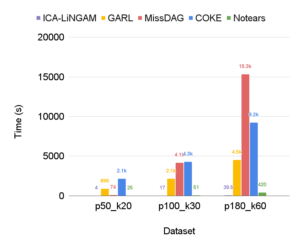
(a) Time complexity.

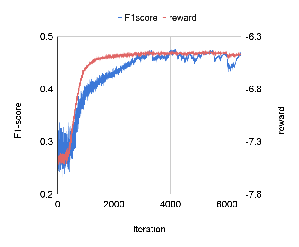
(b) Training process.

Figure 5. Training information in COKE and other baselines.

Execution Time.

Figure 5 (a) shows the training times for each model. MissDAG exhibited a longer training time for numerous variables, indicating inefficiency in high-dimensional causal discovery. In contrast, GARL’s training time increased less with more variables, demonstrating the efficiency of its RL-based architecture. While COKE requires more time in datasets with fewer variables, it significantly reduces processing time compared to MissDAG in datasets with more variables. COKE benefits from RL-based techniques, demonstrating consistent time efficiency up to $p180$.

Visualizations of the Optimization Process.

The designed reward function proves beneficial for causal graph construction, as evidenced by the positive correlation between the F1 score and the reward. In Figure 5 (b), the iteration status between the F1-score and reward during COKE’s training process illustrates this correlation. Despite incorporating an incomplete data process, our model consistently enhances the F1-score and achieves convergence.

5.3. Ablation Study

To evaluate the importance of chronological order (CO), expert knowledge (EK), and the incomplete data process (Incomp.) in our model, we conducted experiments in Table 3. Chronological ordering information is crucial for accurate causal graph construction, as indicated by the significant performance drop observed when this aspect is neglected. This results in inferior performance across all 12 settings, failing to achieve even the second-best result in any of them. The impact of the incomplete data process is significant as the number of variables increases. Specifically, results show a marked decrease in performance when the incomplete data process is not applied to datasets with $p180$ variables. These experiments show the essential roles that chronological order, expert knowledge, and the incomplete data process play in our model, demonstrating their importance in achieving robust results.

6. Conclusion

In this paper, we introduce COKE, a method designed to construct causal graphs by leveraging expert knowledge and chronological order in datasets with high missing values. COKE utilizes manufacturing recipes to maximize the utility of samples with missing values, enabling graph construction without data imputation. By employing the graph attention network, COKE integrates expert knowledge and chronological order into the actor-critic training process. It utilizes the BIC score as a reward function to optimize the graph generation model, eliciting the final causal graph with the maximum reward. Experimental results show that in synthetic data with multiple representative missing proportions and variable counts, COKE outperformed several strong baselines across various settings showcasing the effectiveness of our framework. We believe COKE could flexibly construct causal graphs not only in manufacturing datasets but also in other domains where leveraging knowledge is crucial for establishing accurate causal relationships. In the future, how to build causal graphs using only samples with missing values will be further investigated within this framework, as real-world data often lack complete datasets.

References

- (1)
- Abu-Samah et al. (2015) A Abu-Samah, MK Shahzad, E Zamai, and A Ben Said. 2015. Failure prediction methodology for improved proactive maintenance using Bayesian approach. IFAC-PapersOnLine 48, 21 (2015), 844–851.
- Bühlmann et al. (2013) Peter Bühlmann, Jonas Peters, and Jan Ernest. 2013. CAM: Causal Additive Models, high-dimensional order search and penalized regression. CoRR abs/1310.1533 (2013).
- Clavijo et al. (2021) Nayher Clavijo, Afrânio Melo, Rafael M Soares, Luiz Felipe de O Campos, Tiago Lemos, Maurício M Câmara, Thiago K Anzai, Fabio C Diehl, Pedro H Thompson, and José Carlos Pinto. 2021. Variable selection for fault detection based on causal discovery methods: Analysis of an actual industrial case. Processes 9, 3 (2021), 544.
- Colledani et al. (2014) Marcello Colledani, Tullio Tolio, Anath Fischer, Benoit Iung, Gisela Lanza, Robert Schmitt, and József Váncza. 2014. Design and management of manufacturing systems for production quality. Cirp Annals 63, 2 (2014), 773–796.
- Ezukwoke et al. (2024) Kenneth Ezukwoke, Anis Hoayek, Mireille Batton-Hubert, Xavier Boucher, Pascal Gounet, and Jérôme Adrian. 2024. Big GCVAE: decision-making with adaptive transformer model for failure root cause analysis in semiconductor industry. Journal of Intelligent Manufacturing (2024), 1–16.
- Gao et al. (2022) Erdun Gao, Ignavier Ng, Mingming Gong, Li Shen, Wei Huang, Tongliang Liu, Kun Zhang, and Howard D. Bondell. 2022. MissDAG: Causal Discovery in the Presence of Missing Data with Continuous Additive Noise Models. In NeurIPS.
- Gao and Cai (2023) Yanyang Gao and Qingsong Cai. 2023. A WGAN-based Missing Data Causal Discovery Method. In 2023 4th International Conference on Big Data, Artificial Intelligence and Internet of Things Engineering (ICBAIE). IEEE, 136–139.
- Gharahbagheri et al. (2015) H Gharahbagheri, S Imtiaz, Faisal Khan, and S Ahmed. 2015. Causality analysis for root cause diagnosis in Fluid Catalytic Cracking unit. IFAC-PapersOnLine 48, 21 (2015), 838–843.
- Hagedorn et al. (2022) Christopher Hagedorn, Johannes Huegle, and Rainer Schlosser. 2022. Understanding unforeseen production downtimes in manufacturing processes using log data-driven causal reasoning. J. Intell. Manuf. 33, 7 (2022), 2027–2043.
- Huang et al. (2020) Xiaoshui Huang, Fujin Zhu, Lois Holloway, and Ali Haidar. 2020. Causal discovery from incomplete data using an encoder and reinforcement learning. arXiv preprint arXiv:2006.05554 (2020).
- Huegle et al. (2020) Johannes Huegle, Christopher Hagedorn, and Matthias Uflacker. 2020. How Causal Structural Knowledge Adds Decision-Support in Monitoring of Automotive Body Shop Assembly Lines. In IJCAI. ijcai.org, 5246–5248.
- Ikram et al. (2022) Azam Ikram, Sarthak Chakraborty, Subrata Mitra, Shiv Kumar Saini, Saurabh Bagchi, and Murat Kocaoglu. 2022. Root Cause Analysis of Failures in Microservices through Causal Discovery. In NeurIPS.
- Kwak and Kim (2012) Doh-Soon Kwak and Kwang-Jae Kim. 2012. A data mining approach considering missing values for the optimization of semiconductor-manufacturing processes. Expert Syst. Appl. 39, 3 (2012), 2590–2596.
- Le et al. (2019) Thuc Duy Le, Tao Hoang, Jiuyong Li, Lin Liu, Huawen Liu, and Shu Hu. 2019. A Fast PC Algorithm for High Dimensional Causal Discovery with Multi-Core PCs. IEEE ACM Trans. Comput. Biol. Bioinform. 16, 5 (2019), 1483–1495.
- Lee and Hastie (2015) Jason D Lee and Trevor J Hastie. 2015. Learning the structure of mixed graphical models. Journal of Computational and Graphical Statistics 24, 1 (2015), 230–253.
- Liang et al. (2004) Steven Y Liang, Rogelio L Hecker, and Robert G Landers. 2004. Machining process monitoring and control: the state-of-the-art. J. Manuf. Sci. Eng. 126, 2 (2004), 297–310.
- Marazopoulou et al. (2016) Katerina Marazopoulou, Rumi Ghosh, Prasanth Lade, and David D. Jensen. 2016. Causal Discovery for Manufacturing Domains. CoRR abs/1605.04056 (2016).
- Morales-Alvarez et al. (2022) Pablo Morales-Alvarez, Wenbo Gong, Angus Lamb, Simon Woodhead, Simon Peyton Jones, Nick Pawlowski, Miltiadis Allamanis, and Cheng Zhang. 2022. Simultaneous Missing Value Imputation and Structure Learning with Groups. In NeurIPS.
- Qiao et al. (2024) Jie Qiao, Zhengming Chen, Jianhua Yu, Ruichu Cai, and Zhifeng Hao. 2024. Identification of Causal Structure in the Presence of Missing Data with Additive Noise Model. In AAAI. 20516–20523.
- Qin et al. (2022) Kai Qin, Lei Chen, Jintao Shi, Zhenxing Li, and Kuangrong Hao. 2022. Root cause analysis of industrial faults based on binary extreme gradient boosting and temporal causal discovery network. Chemometrics and Intelligent Laboratory Systems 225 (2022), 104559.
- Rubin (1976) Donald B Rubin. 1976. Inference and missing data. Biometrika 63, 3 (1976), 581–592.
- Shimizu et al. (2006) Shohei Shimizu, Patrik O. Hoyer, Aapo Hyvärinen, and Antti J. Kerminen. 2006. A Linear Non-Gaussian Acyclic Model for Causal Discovery. J. Mach. Learn. Res. 7 (2006), 2003–2030.
- Sim et al. (2014) Hyunsik Sim, Doowon Choi, and Chang Ouk Kim. 2014. A data mining approach to the causal analysis of product faults in multi-stage PCB manufacturing. International journal of precision engineering and manufacturing 15 (2014), 1563–1573.
- Stekhoven and Bühlmann (2012) Daniel J. Stekhoven and Peter Bühlmann. 2012. MissForest - non-parametric missing value imputation for mixed-type data. Bioinform. 28, 1 (2012), 112–118.
- Teyssier and Koller (2005) Marc Teyssier and Daphne Koller. 2005. Ordering-Based Search: A Simple and Effective Algorithm for Learning Bayesian Networks. In UAI ’05, Proceedings of the 21st Conference in Uncertainty in Artificial Intelligence, Edinburgh, Scotland, July 26-29, 2005. AUAI Press, 548–549.
- Tu et al. (2018) Ruibo Tu, Cheng Zhang, Paul Ackermann, Hedvig Kjellström, and Kun Zhang. 2018. Causal discovery in the presence of missing data. CoRR abs/1807.04010 (2018).
- Wang et al. (2021) Xiaoqiang Wang, Yali Du, Shengyu Zhu, Liangjun Ke, Zhitang Chen, Jianye Hao, and Jun Wang. 2021. Ordering-Based Causal Discovery with Reinforcement Learning, Zhi-Hua Zhou (Ed.). ijcai.org, 3566–3573.
- Wang et al. (2020) Yuhao Wang, Vlado Menkovski, Hao Wang, Xin Du, and Mykola Pechenizkiy. 2020. Causal Discovery from Incomplete Data: A Deep Learning Approach. CoRR abs/2001.05343 (2020).
- Yang et al. (2023b) Dezhi Yang, Guoxian Yu, Jun Wang, Zhongmin Yan, and Maozu Guo. 2023b. Causal Discovery by Graph Attention Reinforcement Learning. In Proceedings of the 2023 SIAM International Conference on Data Mining, SDM 2023, Minneapolis-St. Paul Twin Cities, MN, USA, April 27-29, 2023. SIAM, 28–36.
- Yang et al. (2023a) Yu Yang, Sthitie Bom, and Xiaotong Shen. 2023a. A hierarchical ensemble causal structure learning approach for wafer manufacturing. Journal of Intelligent Manufacturing (2023), 1–18.
- Zheng et al. (2018) Xun Zheng, Bryon Aragam, Pradeep Ravikumar, and Eric P. Xing. 2018. DAGs with NO TEARS: Continuous Optimization for Structure Learning. In NeurIPS. 9492–9503.