Testing the cosmic distance duality relation with Type Ia supernova and transverse BAO measurements
Abstract
In this work, we test the cosmic distance duality relation (CDDR) by comparing the angular diameter distance (ADD) derived from the transverse Baryon Acoustic Oscillations (BAO) data with the luminosity distance (LD) from the Pantheon type Ia supernova (SNIa) sample. The binning method and Gaussian process are employed to match ADD data with LD data at the same redshift. First, we use nonparametric and parametric methods to investigate the impact of the specific prior values of the absolute magnitude from SNIa observations and the sound horizon scale from transverse BAO measurements on the CDDR tests. The results obtained from the parametric and non-parametric methods indicate that specific prior values of and lead to significant biases on the CDDR test. Then, to avoid these biases, we propose a method independent of and to test CDDR by considering the fiducial value of as a nuisance parameter and then marginalizing its influence with a flat prior in the analysis. No violation of the CDDR is found, and the transverse BAO measurement can be used as a powerful tool to verify the validity of CDDR in the cosmological-model-independent method.
Cosmic distance duality relation, Parametrization, Cosmological-model-independent method
pacs:
98.80.Es, 95.36.+x, 98.80.-kI Introduction
The cosmic distance duality relation (CDDR) is the most fundamental relationship in modern cosmology, which states that the luminosity distance (LD) and the angular diameter distance (ADD) follow the following relation,
| (1) |
Here, is the redshift of the observed source. This relation is first proved by Etherington Etherington1993 , and it is based on two fundamental hypotheses: (a) the photon always travels along null geodesics in Riemannian geometry; (b) the number of photons is conserved ellis1971 ; ellis2007 . As a fundamental and crucial relation independent of Einstein field equations and the nature of matter, CDDR is widely used to observe the large-scale distribution of galaxies and the near uniformity of the Cosmic Microwave Background (CMB) radiation temperature Aghanim2020 , determine the gas mass density distribution and temperature distribution of galaxy clusters Cao20112 ; Cao2016 , test the geometric shape of galaxy clusters Holanda2011 , and measure the curvature of the universe using strong gravitational lensing systems Liu2020 ; Xia2017 ; Qi2019 . In astronomical observations, any violation of the CDDR implies the existence of new physics or the presence of unexplained errors in the observations. Therefore, it is necessary to test the validity of CDDR through various astronomical observations.
One can in principle check the validity of the CDDR with astronomical observations by comparing the LD with ADD of some objects at the same redshift. In the early stage, due to the lack of observational data, the CDDR test was performed by comparing the observed values with the corresponding theoretical values in the assumed cosmological model. De Bernardis et al. DeBernardis2006 and Uzan et al. Uzan2004 tested CDDR using galaxy cluster samples with the LD from the cosmological constant cold dark matter (CDM) model Reese2002 ; Bonamenteet2006 , and found no violation from the CDDR. Using galaxy cluster data and the conventional CDM model constrained from WMAP (7 years) results, Holanda et al. validated the CDDR with the elliptical and spherical models at and confidence level (CL) Holanda2011 , respectively. Then, Lazkoz et al. verified the effectiveness of CDDR at CL by comparing the dark energy model constraints from the CMB and baryon acoustic oscillation (BAO) with those obtained from the latest type Ia supernova (SNIa) standard candle data at that time Lazkoz2008 . However, any hypothetical cosmological model will bring bias to the testing of CDDR.
With the development of astronomic observations, CDDR can be tested directly by comparing the LD of Type Ia supernovae with the ADD of other astronomical observations in the cosmological-model-independent method. With the galaxy cluster samples Bonamenteet2006 ; DeFilippis05 and SNIa data, Holanda et al. holanda20103 and Li et al. Li2011 performed the CDDR test with adoption of a criterion () and chose the closest one. To avoid the larger statistical errors caused by using only one SNIa data point from all those available that meet the selection criterion, Meng et al. Meng2012 did not use the nearest point from SNIa compilation, they binned the available data (hereafter referred to as binning method) to obtain LD that matches the corresponding ADD sample. They concluded that the marked triaxial ellipsoidal model can better describe the geometrical structure of galaxy cluster than the spherical model if the CDDR is valid. Then, Wu et al. tested CDDR by comparing the Union 2.1 compilation with the five ADD data points from the BAO measurements, and found that the BAO measurement is a very powerful tool to test the CDDR due to the precision of the BAO measurements Wu2015 . Still some other tests, involving the ADD of galaxy clusters, current CMB observations Ellis2013 , Hubble parameter data from cosmic chronometers, gas mass fraction (GMF) measurements in galaxy clusters Goncalves2012 ; Goncalves2015 , strong gravitational lensing (SGL) Cao2012 ; Cao2015 , South Pole Telescope (SPT) Sunyaev–Zel’dovich (SZ) clusters and X-ray Multi-mirror Mission (XMM)-Newton measurements Bocquet2015 ; Bora2021 ; Benson2013 ; Bulbul2019 ; Liu2021 ; McDonald2016 ; Stalder2013 , the x-ray surface brightness observations of galaxy clusters jointly with type Ia supernovae and CMB temperature Holanda201711 ; Luzzi2009 , and time delay lenses Balmes , are performed to investigate the validity of the CDDR by assuming a deformed CDDR, such as , in different redshift range, and the results show that CDDR is consistent with astronomic observations at certain CLs avtidisgous ; Holanda2012a ; Santos2015 ; Stern2010 ; Holanda2012 ; Liao2011 ; Holanda20171 ; Liao2016 ; fuxiangyun ; Fu2017 ; Liang2013 ; Rana ; Ruan ; Xu2022 ; Holanda2017 ; Zheng2020 .
SNIa observations and BAO measurements, as standard candles and standard rulers in astronomical observations, play important roles in the CDDR test. It is worth noting that LD obtained from SNIa observation depends on its peak absolute magnitude , which is considered to be a fixed value that does not vary with other factors. Recently, using the Hubble measurements from the cosmic chronometers, Kumar et al. probed the variability of SNIa along with its correlation with spatial curvature and CDDR Kumar2022 , and they found no evolution of within CL. There have been some other attempts to derive the value of from the cosmological perspective Camarena2020 ; Dinda2023 , and different values of are obtained from the SNIa data with other combinations of datasets, such as CMB observations, the cosmic chronometers data for the Hubble parameter, and BAO observations. It was also found there was a mismatch between the SNIa absolute magnitude calibrated by Cepheids at and Camarena2021 ; Camarena20201 . Recently, hints of possible weak evolution of were also pointed out in Refs. Kazantzidis2021 ; Kazantzidis2020 . In addition, the so-called fitting problem remains a challenge for BAO peak location as a standard ruler Ellis1987 , although BAO measurements are employed to analyze various cosmological parameters. In particular, Roukema et al. recently detected the environmental dependence of BAO location Roukema2015 ; Roukema2016 . Moreover, Ding et al. and Zheng et al. pointed out a noticeable systematic difference between Hubble measurements based on BAO and those obtained with differential aging techniques Ding2015 ; Zheng2016 . Different values of sound horizon scales and the present Hubble parameter are obtained from various observational data, such as CMB observations Ade2016 ; Bennett2013 , the Sloan Digital Sky Survey (SDSS) data release 11 galaxies Carvalho2020 , and BAO measurements Verde2017 . Therefore, any CDDR tests completed by the priors of and are not absolutely independent of cosmological model, as the LD and ADD derived from of SNIa observation and of BAO measurements are dependent on the cosmological model to some extent. In addition, any priors of and may lead to biases in the CDDR tests. Therefore, it is meaningful to investigate the impacts of and on the CDDR tests, and explore new methods that are independent of and to test CDDR, which is the main motivation of this work.
In this work, we perform the CDDR test by comparing LD from Pantheon SNIa data with ADD from transverse BAO data. The function is used to verify possible deviation at any redshift. Using the Gaussian process, we obtain the smoothing LD of SNIa data and the smoothing ADD from the transverse BAO data with priors of the absolute magnitude and the sound horizon scale . We first investigate the impacts of and on CDDR tests by comparing the smoothing LD function with the ADD function in the nonparametric method. Then, with three parametrization for the function , we test CDDR by using the binning method to match the SNIa data with the BAO measurements at the same redshift in the parametric method. The results obtained from the nonparametric and parametric methods show that the priors of and may cause significant biases in the CDDR test. To avoid these bias, we consider variables and as nuisance parameters to determine the LD and ADD, and then adopt a new variable to analytically marginalize its influence with a flat prior in the analysis. We show that CDDR is consistent with the observed data, and the parametric method for testing CDDR is independent of cosmological models.
II Data and Methodology
II.1 Data
To validate CDDR, two types of cosmological distances are usually required, i.e., LD and ADD . In this work, LD data are obtained from the Pantheon SNIa observations, which consists of 1048 data points from the Pan-STARRS1 Deep Survey with the redshift range of Scolnic2018 . The distance modulus of the Pantheon compilation is calibrated from the SALT2 light-curve fitter through applying the Bayesian Estimation Applied to Multiple Species with Bias Corrections method to determine the nuisance parameters and taking account of the distance bias corrections, namely, . Here denotes the peak apparent magnitude observed in the rest-frame B-band, and represents the absolute magnitude. The observational constraints on the cosmological parameters, such as the deceleration parameter, the matter-energy density parameter, and the dark energy density parameter, etc. are estimated based on the value of and Linden2009 ; Camarena2020 . SNIa observations firstly revealed the late time cosmic acceleration Riess1998 ; Perlmutter1999 ; Scolnic2018 , where the observations are based on the fact that SNIa can be considered as a standard candle and its peak absolute magnitude, , is uniform. However the constancy of absolute magnitude of SNIa has often been questioned as an immediate retort to the tension.
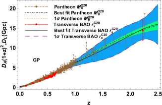
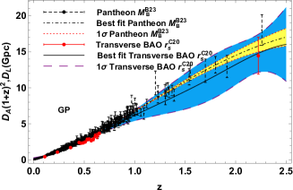
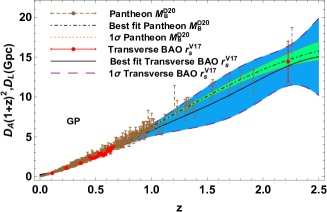
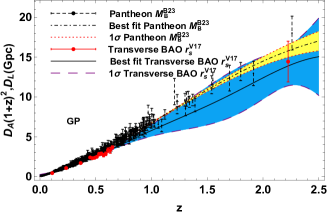
In recent years, several studies have raised the question of whether or not might evolve with redshift. With an inverse distance ladder, the CMB constraint on the sound horizon predicts , while the estimate from SH0ES corresponds to . Hence, we first focus on whether the difference in would affect the CDDR test. In this work, we consider two specific priors of derived from different observational data sets within various redshift ranges, namely, (a) , which was derived from Supercal supernovae in the relative low redshift range by Camarena and Marra Camarena2020 in CDM through a de-marginalization of the SH0ES determination Reid2019 (hereinafter referred to as ); (b) obtained by combining SNIa observations with BAO observations Dinda2023 (hereinafter referred to as ). Considering the observational uncertainty of , the error bar of can be written as . The relation between LD Zhou2019 and distance modulus can be expressed as
| (2) |
and the uncertainty of can be obtained from the following formula /5.
The measurement of the BAO scale is usually obtained by applying the two-point correlation function (2PCF) to a large number of galaxy distributions, where the BAO feature appears as a bump at the corresponding scale. This type of analysis may bias cosmological parameter constraints, since it assumes a fiducial cosmology in order to convert measured angular positions and redshifts into comoving distances. The astronomic observation of the transverse BAO scale can be obtained by using the 2-point angular correlation function (2PACF), which involves only the angular separation between pairs Carvalho2020 . This yields the ADD information almost model-independently, provided that the comoving sound horizon is known Carvalho2020 ; Nunes2020 . The 15 transverse BAO data points in this work are taken from Table I in Ref. Nunes2020 , which were released publicly from the SDSS York2000 . The transverse BAO data set was also employed to test the cosmological principle Arjona2021 ; Bengaly2022 ; Wang2023 . The ADD can be obtained from the transverse BAO data,
| (3) |
Here, is the sound horizon scale at the drag epoch, and corresponds to the comoving observed angle from the transverse BAO measurements.
However, the value of sound horizon scale is dependent on the Hubble constant (as a local anchor of the cosmic distance scale), and different values of are obtained from various astronomic observations. Recently, the sound horizon scale was calibrated from CMB observations in the high redshift region , i.e., and from the most recent Planck Ade2016 and WMAP9 Bennett2013 measurements, respectively. In addition, using the SDSS data release 11 galaxies and the prior of the matter density parameter given by the SNIa data, Carvalho et al. obtained constraint on (hereafter referred to as ) at the relatively low redshift Carvalho2020 ,
| (4) |
Here, is the Hubble constant in units of . Verde et al. also obtained the sound horizon (referred to as ) with SNIa and BAO measurements Verde2017 ,
| (5) |
We adopt the prior values of the sound horizon and , which are obtained from different astronomic observations at the relatively low redshifts, to further investigate the impact of on the CDDR test. In fact, the value of is also related to the observed value of the Hubble constant . However, there are differences in the measurements of the Hubble constant from astronomic observations, known as the Hubble tension (the discrepancy between the local measurements based on cepheid variables and SNIa and CMB analysis within the context of the CDM model). For simplicity and the consistency of observational SNIa data, we use the Hubble constant , which was obtained from a Cepheid-only calibration of SNIa data points with good quality Riess2022 , to investigate the impacts of and on the CDDR tests.
II.2 Gaussian process and Binning method
To test the validity of CDDR, the direct method is to make the comparison between ADD and LD from various observations at the same redshift. Due to the lack of the astronomic observational data, different methods are employed to match ADD with LD at the same redshift. Here, we employ two cosmological model-independent methods, namely the Gaussian process and the binning method, to perform this task.
We reconstruct the LD or ADD as a smoothing function from SNIa observations or transverse BAO measurements with the Gaussian process Seikel2012 ; Carlos2020 ; Shafieloo2012 . Gaussian process can be used for reconstructing a function given function values under the assumption of probability distribution, assuming a probability distribution for finite-dimensional random variables. It also employs a kernel function and covariance function . Different choices for kernels may lead to slightly more degenerate reconstruction, thereby reducing the statistical significance of these deviations Bengaly2022 . More recently, Bayes factors were used to evaluate the differences between different kernels with the cosmic chronometer data, SNIa, and gamma ray burst, and it showed that Bayes factors indicate no significant dependence of the data on the kernels Zhang2023 . Here, we ignore the influences of different kernels and choose the general covariance kernel, namely, the squared exponential Seikel2012 ,
| (6) |
and are the hyper-parameters in the fit. represents a measure of the correlation length of the correlation that provides the width of the reconstructed curve, denotes the typical variation in function values, and and represent two different points in space Seikel2012 . GP has been widely applied in cosmology, such as for tests on cosmological constants with supernovae Yahya2014 , constraints on the dark energy equation of state Seikel2012 and cosmological mixing parameters Mukherjee2021 ; Holanda2013 , tests on the Cosmological Principle Wang2023 , and inference of the Hubble constant Li2016 ; Verde2014 ; Busti2014 . The reconstructed results derived from different priors of are shown in Fig. 1.
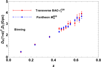
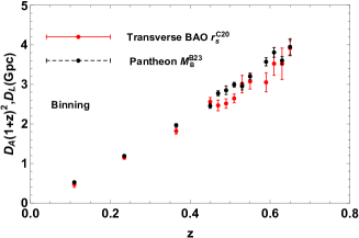
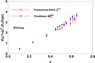
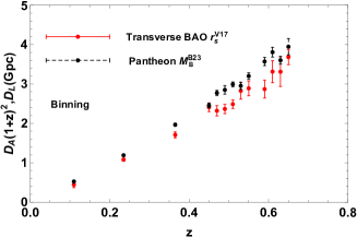
To verify the validity of CDDR, instead of choosing the nearest SNIa data to match SNIa observation with ADD measurements at the same redshift with a selection criterion proposed in Refs. holanda20103 ; Li2011 ; Liao2016 , we bin the available data from SNIa data points that meet the selection criterion. This method, named the binning method, may be used to avoid the statistical errors resulting from merely one SNIa data point with all those available that meet the selection criterion, and has been used to discuss the CDDR tests in Refs. Wu2015 ; Meng2012 . Here, we adopt an inverse variance weighted average of all the selected data, and select the LD data points from SNIa observation through a procedure. Once the data points have been matched with the BAO sample, they will no longer be used to avoid the SNIa-to-SNIa correlations between individual CDDR test. The weighted mean LD and its uncertainty can be obtained with conventional data reduction techniques in Chapter.() of the Ref. Bevington ,
| (7) |
| (8) |
Here, denotes the th appropriate luminosity distance data points, and corresponds its observational uncertainty.
In this work, we choose Pantheon SNIa data points and match them with the transverse BAO data points, as the number of Pantheon SNIa far exceeds the number of BAO measurements. Only 13 data points in BAO measurements meet the selection criteria. Data points at and are discarded. The distribution of the transverse BAO data and SNIa data is shown in Fig. 2.
II.3 Methodology
We adopt the function to verify the possible deviations from CDDR at any redshifts by comparing the from SNIa with the from transverse BAO measurements. can be obtained with the following expression,
| (9) |
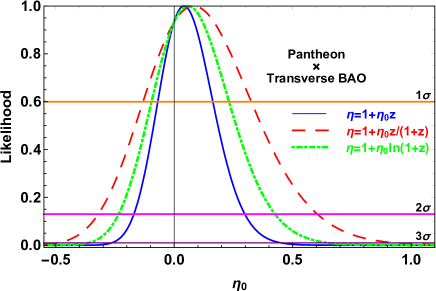
At any redshift, implies a discrepancy between CDDR and the astronomic observations. We first obtain the function at any redshifts by comparing the smoothing ADD with the LD at the same redshift, where and are obtained with different priors and . It is obvious that this method of the CDDR test is nonparametric, and the results are shown in Fig. 3.
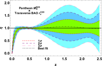
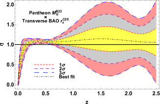
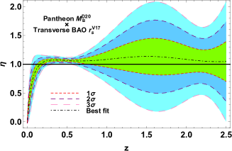
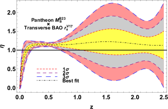
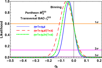
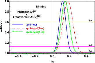
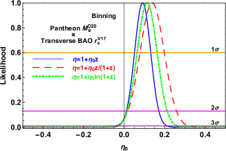
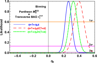
The parametric method plays an important role in testing CDDR. We adopt three parameterizations for , namely a linear form P1: and two non-linear forms P2: , and P3: . Any denotes the deviation between CDDR and the observational data. The observed is obtained from Equ. 9, and the corresponding error can be written as
| (10) |
Thus, we obtain
| (11) |
Here, denotes the number of the available transverse BAO data points with the binning method. The results of constraints on are shown in Fig. 4 and Tab. 1.
| parmetrization | P1: | P2: | P3: |
|---|---|---|---|
It is easy to see that the results obtained from the nonparametric and parametric methods depend on the priors of the and . To test CDDR with a method independent of absolute magnitude and sound horizon scale , we consider fiducial values of and as nuisance parameters to determine LD and ADD , and marginalize their influences with flat priors in the analysis. The likelihood distribution can be rewritten as
| (12) |
Here, , , , and
| (13) |
Because the uncertainties of individual SNIa or the BAO measurements do not depend on or , it is possible to remove these parameters from our fits by analytically marginalizing over them. Therefore, following the method described in Ref. Xu2022 ; Wang2023 ; Conley2011 , we marginalize analytically the likelihood function over , and obtain
| (14) |
where , , and . It is easy to see that the in Equ. 14 is independent of the parameters and . The results are shown in Fig. 6 and Table 1. It is worth noting that, the CDDR test in this work is also independent of the Hubble constant , as is marginalized in the analysis. To assess the ability of transverse BAO measurements to constrain parameters , we also include the results obtained from other observational data in Table 2.
| Dataset used | P1: | P2: | P3: |
|---|---|---|---|
| Li2011 | |||
| Goncalves2015 | |||
| Wu2015 | |||
| Wu2015 | |||
| Bora2021 | |||
| Holanda2017 | |||
| Xu2020 | |||
| Xu2022 |
III Results and Analysis
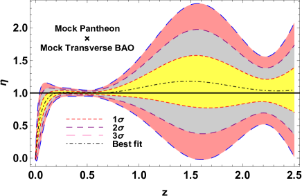
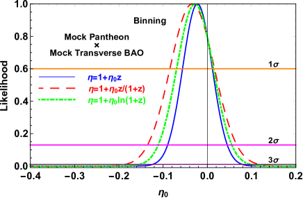
To show the robustness of nonparametric and parametric methods, we also conduct an unbiased test by generating mock data for and that strictly adheres to . The redshifts and uncertainties are taken from the actual observational Pantheon and transverse BAO data. The fiducial LDs () or ADDs () of the mock data are obtained from a known flat CDM with the most recent Planck results Ade2016 . The simulated measurements of or can be derived from the random normal distribution through the equation . The results are shown in Fig. 6, and it can be concluded that CDDR is consistent with the mock data at CL from the parametric and nonparametric methods. The possible deviations from the CDDR at any redshifts can be validated using the nonparametric method.
As shown in Fig. 3, for the reconstructed results with the nonparametric methods, within the redshift range , the deviations of the value of function from may be due to the lack of the observed transverse BAO data points. CDDR is consistent with the observational data at CL with the priors of and , at CL with the prior of and , and at CL marginally with the priors of and , respectively. However, with the priors of and , the results indicate that there is a strong deviation between the CDDR and the observed data in the redshift region where most of the observed transverse BAO data are located. Thus, the priors of and will cause significant bias in the CDDR test.
From Fig. 4 and Tab. 1, the results obtained with the three types of parameterizations from the binning method are consistent with that from the nonparametric method. Our results indicate a stronger violation from CDDR than that obtained from Ref. Kumar2022 , where the CDDR was fairly consistent with different best fitted value of from Pantheon SNIa and Hubble data at CL in both flat and a non-flat universe. Thus, the parametric method provides an effective way to check the CDDR through constraining the parameter .
Afterwards, we use the Akaike Information Criterion (AIC) Akaike1974 and Bayesian Information Criterion Schwarz1978 to compare the results obtained from the three parameterizations. The AIC and the BIC are defined as the following forms, respectively,
| (15) |
| (16) |
Here, denotes the value of the maximum likelihood estimate, represents the number of free parameters of the model, and is the total number of data points. The results are listed in Tab. 3. In all of the cases, the value of for the parametrization P2 is the smallest one among the three parameterizations, although the parametrization P1 provides the most stringent constraints on the test of CDDR. We can get that all the value of , and we cannot determine which parametrization is the most appropriate one, since indicates a weak evidence in favour of the reference model, which still leaves the question of which model is the most appropriate Akaike1974 ; Schwarz1978 .
Now, we compare the capability of transverse BAO measurements with those obtained from other astronomical observations, where specific priors of cosmological variables are used. The transverse BAO measurements improve the accuracy of about 65% at CL by comparing with the results obtained from the Union2+galaxy cluster observation (the elliptical model) Li2011 or Union2.1+91GMF observation Goncalves2015 , and about 40% at CL by comparing with the results obtained from Union2.1+BAO measurements Wu2015 , where the CDDR tests were performed with the specific priors of or from the CMB observations. Our results are about 25% more stringent than the constraints on from the SPT-SZ clusters and X-ray measurements from XMM-Newton Bora2021 , where the prior of and are used. Our results are also comparable with that obtained from the x-ray GMF of galaxy clusters jointly with SNIa and CMB temperature Holanda2017 , where the is fixed to derive the LD.
As for the case of testing CDDR with a flat prior of , the CDDR is compatible with the observed data at CL. The constraints on at CL are much weaker than those obtained with the specific priors of and . In addition, we marginalize and separately with the same observational data, and we obtain the same results as those obtained with the method by marginalizing . Therefore, our method of combining two variables into one parameter can reduce the computational complexity arising from integration, and it cannot provide stricter constraints on the parameters. We also perform the CDDR tests with the unanchored LD from Pantheon SNIa while , where is fixed as from Ref. Riess2016 . We get that the results obtained by marginalizing and are similar to those obtained by marginalizing and . To explore the capability of testing CDDR with the transverse BAO measurements, it is meaningful to compare our results with the previous constraints on from different data sets by marginalizing certain parameters with a flat prior. The transverse BAO measurements improve the accuracy of about 50% at CL by comparing with the results obtained from the Union2.1+BAO observations, where the dimensionless Hubble constant was marginalized with a flat prior Wu2015 . The constraints on are comparable with that obtained from the latest Pantheon sample and BOSS DR12 BAO measurements in the redshift region Xu2020 or from five BAO measurements from the extended Baryon Oscillation Spectroscopic Survey data release 16 quasar sample with the Pantheon SNIa samples Xu2022 where the and were marginalized. Therefore, the ability to test CDDR from the transverse BAO observations is at least comparable to that of previous BAO observations. In addition, it is worth mentioning that in Ref. Kumar2022 , the CDDR test was performed through making constraints on , spatial curvature () and CDDR parameter (), resulting different best fitted value and spatial curvature (). In our analysis, the parametric method used to test CDDR is not only independent of cosmological model, but also independent of the absolute magnitude from SNIa observation, sound horizon scale of BAO measurements, and Hubble constant .
| parmetrization | parmetrization | ||||||||||
|---|---|---|---|---|---|---|---|---|---|---|---|
IV conclusion
CDDR plays an important role in astronomic observations and modern cosmology, and any deviation from CDDR may imply a signal of exotic physics. SNIa and BAO measurements can be considered effective observational data for testing CDDR, as they can provide precise LD and ADD data. Due to the uncertainty in determining the absolute magnitude from different astronomical observations, as well as the uncertainty in the sound horizon scale in the fitting problem of BAO observation, it is necessary to investigate the impact of the quantities and from SNIa and BAO observations on the CDDR test, and use new BAO measurements and more reliable methods to check the validity of the CDDR.
In this work, we first, use a nonparametric method to test CDDR by comparing the LD obtained from the Pantheon SNIa compilation with ADD from transverse BAO measurements. The function is adopted to probe the possible deviations from CDDR at any redshift. We use the two prior values of the absolute magnitude and sound horizon scale , respectively, to obtain the LD of the SNIa observation and ADD of the transverse BAO measurements. The smoothing functions of LD and ADD are reconstructed with the Gaussian process. The results show that the different priors of and will cause significant bias in testing CDDR.
Then, we employ three parameterizations to describe the function that evolves with the redshift , namely P1: , P2: , and P3: , and test CDDR by constraining the parameter with the priors of and . Our results show that P1 offers the best rigorous constraints on the parameter among the three parameterizations. Compared with the results from the nonparametric method, the same results are obtained from the nonparametric method for the observational data and the priors of and . Therefore, the parametric method offers an effective way to test CDDR by constraining the parameter . The results also imply that in the test of CDDR, some bias might be caused by the priors of and when the exact values of observation and are not determined.
To avoid the bias caused by the priors of and in the CDDR test, we consider fiducial values of and as nuisance parameters to determine the LD and ADD from the astronomic observations, and then marginalize their influences with a flat prior of new variable in the analysis. We match the SNIa data with the transverse BAO measurements at the same redshift with the binning method. Our results show that CDDR is consistent with the current observational data at CL, and the ability of observational data with this method to constrain the parameter is weaker than that obtained from the specific values of and . The reason is that there is one more degree of freedom in our analysis compared to the previous analysis. Compared with previous results from other astronomic observations, the capability of the transverse BAO observation to test the CDDR is at least comparable to previous observations, whether using the method independent of and or the method dependent of and . It is meaningful to note that this method to test CDDR is not only independent of cosmological models, but also independent of the prior values of absolute magnitude and sound horizon scale . In addition, with the developments of the BAO measurements, the neutral hydrogen intensity mapping technique can be used to measure the BAO signals more efficiently, and 200 observational data in the redshift region will be realized in the coming decades Zhang2020 . As the quality and quantity of measurements for SNIa and BAO measurements increase, the parametric method in our analysis will be a powerful way to test CDDR independent of both the cosmological model and the values of and . Thus, the transverse BAO measurements can be used as a powerful tool to test CDDR.
Acknowledgements.
We very much appreciate helpful comments and suggestions from anonymous referees, and helpful discussion from Hongwei Yu and Puxun Wu. This work was supported by the National Natural Science Foundation of China under Grants No. 12375045, No. 12305056, No. 12105097, and No. 12205093, the Hunan Provincial Natural Science Foundation of China under Grants No. 12JJA001 and No. 2020JJ4284, the Natural Science Research Project of Education Department of Anhui Province No. 2022AH051634, and the Science Research Fund of Hunan Provincial Education Department No. 21A0297.References
- (1) I. M. H. Etherington, Phil. Mag. 15, 761 (1933); reprinted in Gen. Rel. Grav. 39, 1055 (2007).
- (2) G. F. R. Ellis, Gen. Rel. Grav. 41, 581 (2009).
- (3) G. F. R. Ellis, Gen. Rel. Grav. 39, 1047 (2007).
- (4) N. Aghanim, Y. Akrami, M. Ashdown, et al., Astron. Astrophys. 641, A6 (2020).
- (5) S. Cao, M. Biesiada, X. Zheng, et al., Mon. Not. R. Astron. Soc. 457, 281 (2016).
- (6) S. Cao and N. Liang, Res. Astron. Astrophys 11, 1199 (2011), arXiv:1104.4942 [astro-ph.CO].
- (7) R. F. L. Holanda, J. A. S. Lima, and M. B. Ribeiro, Astron. Astrophys. 528, L14 (2011).
- (8) T. Liu, S. Cao, J. Zhang, et al., Mon. Not. R. Astron. Soc. 496, 708 (2020).
- (9) J. Q. Xia, H. Yu, G. J. Wang, et al., Astrophys. J. 834, 75 (2017).
- (10) J. Z. Qi, S. Cao, S. Zhang, et al., Mon. Not. R. Astron. Soc. 483, 1104 (2019).
- (11) F. DeBernardis, E. Giusarma, A. Melchiorri, et al., Int. J. Mod. Phys. D 15, 759 (2006), arXiv:gr-qc/0606029.
- (12) J. P. Uzan, N. Aghanim, and Y. Mellier, Phys. Rev. D 70, 083533 (2004), arXiv:astro-ph/0405620.
- (13) E. D. Reese, J. E. Carlstrom, M. Joy, et al., Astrophys. J. 581, 53 (2002).
- (14) M. Bonamenteet, M. K. Joy, S. J. LaRoque, et al., Astrophys. J. 647, 25 (2006).
- (15) R. Lazkoz, S. Nesseris, and L. Perivolaropoulos, J. Cosmol. Astropart. Phys. 07 (2008) 012, arXiv:0712.1232.
- (16) E. De Filippis, M. Sereno, M. W. Bautz, et al., Astrophys. J. 625, 108 (2005).
- (17) R. F. L. Holanda, J. A. S. Lima, and M. B. Ribeiro, Astrophys. J. 722, L233 (2010).
- (18) Z. Li, P. Wu, and H. Yu, Astrophys. J. Lett. 729, L14 (2011).
- (19) X. L. Meng, T. J. Zhang, H. Zhan, et al., Astrophys. J. 745, 98 (2012).
- (20) P. X. Wu, Z. X. Li, X. L. Liu, et al., Phys. Rev. D 92, 023520, (2015).
- (21) G. F. R. Ellis, R. Poltis, J. P.Uzan, et al., Phys. Rev. D 87, 103530 (2013).
- (22) R. S. Gonçalves, R. F. L. Holanda, and J. S. Alcaniz, Mon. Not. R. Astron. Soc. 420, L43 (2012).
- (23) R. S. Goncalves, A. Bernui, R. F. L. Holanda, and J. S. Alcaniz, Astron. Astrophys. 573, A88 (2015).
- (24) S. Cao, Y. Pan, M. Biesiad, et al., J. Cosmol. Astropart. Phys. 03 (2012) 016.
- (25) S. Cao, M. Biesiada, R. Gavazzi, et al., Astrophys. J. 806, 185 (2015), arXiv:1509.07649.
- (26) S. Bocquet, A. Saro, J. J. Mohr, et al., Astrophys. J. 799, 214 (2015).
- (27) K. Bora and S. Desai, J. Cosmol. Astropart. Phys. 06 (2021) 052, arXiv:2104.00974.
- (28) B. A. Benson, T. De Haan, J. P. Dudley, et al., Astrophys. J. 763, 147 (2013).
- (29) E. Bulbul, I. N. Chiu, J. J. Mohr, et al., Astrophys. J. 871, 50 (2019).
- (30) Z. E. Liu, W. F. Liu, T. J. Zhang, et al., Astrophys. J. 922, 19 (2021).
- (31) M. McDonald, E. Bulbul, T. De Haan, et al., Astrophys. J. 826, 124 (2016).
- (32) B. Stalder, J. Ruel, M. Brodwin, et al., Astrophys. J. 763, 93 (2013).
- (33) R. F. L. Holanda, S. H. Pereira, and S. S. da Costa, Phys. Rev. D 95, 084006 (2017).
- (34) G. Luzzi, M. Shimon, L. Lamagna, Y. Rephaeli, M. De Petris, A. Conte, S. De Gregori, and E. S. Battistelli, Astrophys. J. 705, 1122 (2009); R. Srianand, P. Petitjean, and C. Ledoux, Nature (London) 408, 931 (2000); G. Hurier, N. Aghanim, M. Douspis, and E. Pointecouteau, Astron. Astrophys. 561, A143 (2014).
- (35) I. Balmes and P. S. Corasaniti, Mon. Not. R. Astron. Soc. 431 1528, (2013), arXiv:1206.5801.
- (36) A. Rana, D. Jain, S. Mahajan, et al., J. Cosmol. Astropart. Phys. 07 (2017) 010.
- (37) C. Ruan, F. Melia, and T. Zhang, Astrophys. J. 866, 31 (2018), arXiv:1808.09331 [astro-ph.CO].
- (38) A. Avgoustidis, C. Burrage, J. Redondo, et al., J. Cosmol. Astropart. Phys. 10 (2010) 024.
- (39) D. Stern, R. Jimenez, M. Kamionkowski, et al., J. Cosmol. Astropart. Phys. 02 (2010) 008.
- (40) R. F. L. Holanda, R. S. Gonçalves, and J. S. Alcaniz, J. Cosmol. Astropart. Phys. 06 (2012) 022.
- (41) S. Santos-da-Costa, V. C. Busti, and R. F. L. Holanda, J. Cosmol. Astropart. Phys. 10 (2015) 061.
- (42) R. F. L. Holanda, J. C. Carvalho, and J. S. Alcaniz, J. Cosmol. Astropart. Phys. 04 (2013) 027.
- (43) K. Liao, Z. Li, J. Ming, et al., Phys. Lett. B 718, 1166 (2013).
- (44) R. F. L. Holanda, V. C. Busti, F. S. Lima, et al., J. Cosmol. Astropart. Phys. 09 (2017) 039.
- (45) X. Y. Fu, P. X. Wu, H. W. Yu, et al., Research in Astron. Astrophys, 11, 895 (2011).
- (46) X. Fu and P. Li, Int. J. Mod. Phys. D 26, 1750097 (2017), arXiv:1702.03626 [gr-qc].
- (47) N. Liang, Z. Li, P. Wu, et al., Mon. Not. R. Astron. Soc. 436, 1017 (2013).
- (48) R. F. L. Holanda, S. H. Pereira, and S. Santos-da-Costa, Phys. Rev. D 95, 084006 (2017), arXiv:1612.09365.
- (49) K. Liao, Z. Li, S. Cao, et al., Astrophys. J. 822, 74 (2016).
- (50) B. Xu, Z. Wang, K. Zhang, et al., Astrophys. J. 939, 115 (2022), arXiv:2212.00269.
- (51) X. Zheng, K. Liao, M. Biesiada, et al., Astrophys. J. 892, 103 (2020).
- (52) D. Kumar, A. Rana, D. Jain, et al., J. Cosmol. Astropart. Phys. 01 (2022) 053.
- (53) D. Camarena and V. Marra, Mon. Not. R. Astron. Soc. 495, 2630 (2020).
- (54) B. R. Dinda and N. Banerjee, Phys. Rev. D 107, 063513 (2023).
- (55) D. Camarena and V. Marra, Mon. Not. R. Astron. Soc. 504, 5164 (2021).
- (56) D. Camarena and V. Marra, Phys. Rev. Research 2, 013028 (2020).
- (57) L. Kazantzidis, H. Koo, S. Nesseris, et al., Mon. Not. R. Astron. Soc. 501, 3421 (2021).
- (58) L. Kazantzidis and L. Perivolaropoulos, Phys. Rev. D 102, 023520 (2020).
- (59) G. F. R. Ellis and W. Stoeger, Classical Quantum Gravity 4, 1697 (1987).
- (60) B. Roukema, T. Buchert, J. J. Ostrowski, et al., Mon. Not. R. Astron. Soc. 448, 1660 (2015).
- (61) B. Roukema, T. Buchert, H. Fuji, et al., Mon. Not. R. Astron. Soc. 456, L45 (2016).
- (62) X. Ding, M. Biesiada, S. Cao, et al., Astrophys. J. Lett. 803, L22 (2015).
- (63) X. Zheng, X. Ding, M. Biesiada, et al., Astrophys. J. 825, 17 (2016).
- (64) P. A. R. Ade, N. Aghanim, M. Arnaud, et al., Astron. Astrophys. 594, A15 (2016).
- (65) C. L. Bennett, D. Larson, J. L. Weiland, et al., Astrophys. J. Suppl. ser. 208, 20 (2013).
- (66) G. C. Carvalho, A. Bernui, M. Benetti, et al., Astropart. Phys. 119, 102432 (2020), arXiv:1709.00271.
- (67) L. Verde, J. L. Bernal, A. F. Heavens, et al., Mon. Not. R. Astron. Soc. 467, 731 (2017), arXiv:1607.05297.
- (68) D. M. Scolnic, D. O. Jones, A. Rest, et al., Astrophys. J. 859, 101 (2018), arXiv:1710.00845 [astro-ph.CO].
- (69) S. Linden, J. M. Virey, and A. Tilquin, Astron. Astrophys. 506, 1095 (2009).
- (70) A. G. Riess, A. V. Filippenko, P. Challis, et al., Astrophys. J. 116, 1009 (1998), arXiv:astro-ph/9805201.
- (71) S. Perlmutter, G. Aldering, G. Goldhaber, et al., Astrophys. J. 517, 565 (1999), arXiv:astro-ph/9812133.
- (72) M. J. Reid, D. W. Pesce, and A. G. Riess, Astrophys. J. Lett. 886, L27 (2019).
- (73) L. Zhou, X. Fu, Z. Peng, et al., Phys. Rev. D 100, 123539 (2019), arXiv:1912.02327.
- (74) R. C. Nunes, S. K. Yadav, J. F. Jesus, et al., Mon. Not. R. Astron. Soc. 497, 2133 (2020), arXiv:2002.09293.
- (75) D. G. York, J. Adelman, J. E. Anderson, et al., Astrophys. J. 120, 1579 (2000).
- (76) R. Arjona and S. Nesseris, Phys. Rev. D 103, 103539 (2021).
- (77) C. Bengaly, Phys. Dark Univ. 35, 100966 (2022), arXiv:2111.06869.
- (78) M. Wang, X. Fu, B. Xu, et al., Phys. Rev. D 108, 103506 (2023).
- (79) A. G. Riess, W. Yuan, L. M. Macri, et al., Astrophys. J. Lett. 934, L7 (2022), arXiv:2112.04510.
- (80) C. A. P. Bengaly, Mon. Not. R. Astron. Soc. 499, L6 (2020), arXiv:1912.05528.
- (81) A. Shafieloo, A. G. Kim, and E. V. Linder, Phys. Rev. D 85, 123530 (2012), arXiv:1204.2272.
- (82) M. Seikel, C. Clarkson, and M. Smith, J. Cosmol. Astropart. Phys. 06 (2012) 036, arXiv:1204.2832.
- (83) H. Zhang, Y. -C. Wang, T. -J. Zhang, et al., Astrophys. J. Suppl. Ser. 266, 27 (2023), arXiv:2304.03911.
- (84) S. Yahya, M. Seikel, C. Clarkson, et al., Phys. Rev. D 89, 023503 (2014), arXiv:1308.4099.
- (85) P. Mukherjee and N. Banerjee, Eur. Phys. J. C 81, 36 (2021), arXiv:2007.10124.
- (86) R. F. L. Holanda, J. C. Carvalho, and J. S. Alcaniz, J. Cosmol. Astropart. Phys. 04 (2013) 027, arXiv:1207.1694.
- (87) Z. Li, J. E. Gonzalez, H. Yu, et al., Phys. Rev. D 93, 043014 (2016), arXiv:1504.03269.
- (88) L. Verde, P. Protopapas, and R. Jimenez, Phys. Dark Univ. 5, 307 (2014), arXiv:1403.2181.
- (89) V. C. Busti, C. Clarkson, and M. Seikel, Mon. Not. R. Astron. Soc. 441, L11 (2014), arXiv:1402.5429.
- (90) P. R. Bevington, D. K. Robinson, J. M. Blair, et al., Computers in Physics, 7 415 (1993).
- (91) A. Conley, J. Guy, M. Sullivan, et al., Astrophys. J. Suppl. Ser. 192, 1 (2011).
- (92) B. Xu and Q. H. Huang, Eur. Phys. J. Plus, 135, 447 (2020).
- (93) H. Akaike, IEEE Trans. Automat. Contr., 19, 716 (1974).
- (94) G. Schwarz, Ann. Stat., 6, 461 (1978).
- (95) A. G. Riess, L. M. Macri, S. L. Hoffmann, et al., Astrophys. J. 56, 826 (2016).
- (96) M. Zhang, B. Wang, et al., Astrophys. J. 918, 56 (2021); P.-J. Wu and X. Zhang, J. Cosmol. Astropart. Phys. 01(2022)060.