Urban Traffic Forecasting with Integrated Travel Time and Data Availability in a Conformal Graph Neural Network Framework

Abstract

Traffic flow prediction is a big challenge for transportation authorities as it helps in planning and developing better infrastructure. State-of-the-art models often struggle to consider the data in the best way possible, intrinsic uncertainties, and the actual physics of the traffic. In this study, we propose a novel framework to incorporate travel times between stations into a weighted adjacency matrix of a Graph Neural Network (GNN) architecture with information from traffic stations based on their data availability. To handle uncertainty, we utilized the Adaptive Conformal Prediction (ACP) method that adjusts prediction intervals based on real-time validation residuals. To validate our results, we model a microscopic traffic scenario and perform a Monte-Carlo simulation to get a travel time distribution for a Vehicle Under Test (VUT) while it is navigating the traffic scenario, and this distribution is compared against the actual data. Experiments show that the proposed model outperformed the next best model by approximately 24% in MAE and 8% in RMSE and validation showed the simulated travel time closely matches the 95th percentile of the observed travel time value.

I INTRODUCTION

Traffic congestion in cities is a big problem. They impact our daily commutes longer, increase pollution, and generally make urban life difficult. According to INRIX, the average time a U.S. person spent was 51 hours just sitting in traffic in 2022 — 15 hours more than in 2021 due to the pandemic but it was 99 hours in 2019 [1]. So, it is a time as well as a monetary loss. Knowing the traffic conditions a-priori can help in making better plans and avoiding congestion. Conventionally, studies have been conducted to predict traffic using historical data and statistical methods, which might not be able to capture the complex dynamics of a traffic scenario.

Lately, there has been a lot of progress in using machine learning, especially in understanding patterns in a spatio-temporal, to get better at predicting how traffic will behave. By looking at roads like a network of nodes and edges (like a map) and using models that are good at handling sequences of data (like how traffic changes throughout the day), we can make smarter decisions. Specifically, using spatial models like Graph Neural Network (GNN) (which are appropriate for mapping out roads and intersections) with a model that can handle the time-varying nature of traffic such as a Recurrent Neural Network (RNN) can help tackle the complexities of forecasting traffic.

However, even with advancements in the spatio-temporal domain, it is an arduous task to perfectly match these models with the actual physics, the associated uncertainties, and how the data is used in the best way possible to make traffic-related predictions. We leveraged Graph Convolution Network (GCN) with a Long Short-Term Memory (LSTM) architecture, inspired by Bing et al. [2], in this study. GCN is a type of GNN that applies the Convolutional Neural Network (CNN) concept in graph-structured data. It can perform a convolutional operation directly on the graph nodes and their neighboring nodes. The fundamental idea is to aggregate features of a selected node and its neighbors within an adjacency matrix. We propose to use travel times between nodes and their neighbors to make the graph model reflect a sense of realism. This helps us understand not just the layout of the roads but also how long it takes to get from one point to another. An LSTM architecture is used as they are known for their ability to capture long-term dependencies in sequential data which includes memory cells and gating mechanisms. This helps them to remember information over long sequences, addressing the vanishing gradient problem common in traditional RNNs.

We also look at the type of data coming from stations that may have a continuous count for the whole year with high granularity known as Continuous Count Stations (CCS) and some may be coarse known as Non-Continuous Count Stations (N-CCS). CCS provides detailed traffic counts for every 15/30/60 minutes for each day throughout the entire year whereas, N-CCS has limited data consisting of traffic counts for just a week or two, or scattered days, which, despite their sparsity, can still provide valuable insights for the traffic flow in that area. By using a weighting strategy to combine all this information, our model can make better predictions. Along with the predictions, uncertainty comes along so we used an adaptive version of conformal prediction known as ACP technique to deal with it. ACP is capable of providing dynamic prediction intervals or uncertainty bounds that adapt over time in a training model. Following this, a microscopic traffic scenario is modeled in SUMO (Simulation of Urban MObility) from the uncertain bounds of the predicted traffic flows. The validation is conducted through a Monte-Carlo simulation and analyzing the VUT travel time distribution against the actual data.

The rest of this paper is organized as follows: Section 2 gives a comprehensive overview of the literature in this field. Section 3 discusses the methodology adopted followed by Section 4, describing the experiments and results. Finally, conclusions are presented in Section 5.

II Related Work

II-A Spatio-Temporal Models

Considerable work has gone into creating a specialized model in the subject of spatio-temporal traffic prediction that can handle both spatial and temporal dynamics for forecasting many different traffic states, including travel demand, trip duration, traffic speed, and traffic flow. In 2017, two prominent models were introduced: the Diffusion Convolutional Recurrent Neural Network (DCRNN) model [3] and the Spatio-Temporal Graph Convolutional Network (STGCN) model [2]. DCRNN used a diffusion process in conjunction with recurrent neural networks to control temporal dependencies, whereas STGCN integrated graph convolutions with gated temporal convolutions.

In 2019, the Temporal Graph Convolutional Network (T-GCN) was developed to improve the integration of spatial and temporal aspects in the traffic forecasts by combining graph convolutions with gated recurrent units [4]. In order to better capture dynamic traffic patterns, attention mechanisms were concurrently added by the Attention-based Spatial-Temporal Graph Convolutional Networks (ASTGCN) [5]. The Graph Multi-Attention Network (GMAN) and Graph WaveNet were also developed around this time and they improved the model in terms of managing intricate spatial-temporal interactions by utilising various attention processes [6], [7]. Bi-component graph convolutions and the integration of graph convolution into LSTM cells were introduced by other models such as the Temporal Graph Convolutional Long Short-Term Memory (TGC-LSTM) network and the Multi-range Attentive Bicomponent Graph Convolutional Network (MFFB) [8], [9]. We also saw the introduction of the Spatio-Temporal Meta learning framework (ST-MetaNet), applying meta-learning to spatio-temporal prediction, and the Dynamic Graph Convolutional Network (DGCN), which adjusted graph convolutional operations for constantly changing graphs [10], [11]. Then came Multi-Weighted Temporal Graph Convolutional network (MW-TGC) that refined spatial-temporal modeling even further by bringing in new ways to weigh temporal relationships and melding them with LSTM architectures [12]. Another study introduced the Structure Learning Convolution (SLC) framework [13] which bolstered teh traditional CNN architecture by incorporating structural information into the convolutional process and made it a versatile tool for learning on graphs.

In order to accommodate the dynamic nature of traffic, more recently, between 2021 and 2022, models like the Time-aware Multi-Scale Graph Convolutional Network (TmS-GCN) and the Attention-Accumulated Graph Recurrent Neural Network (AAGRNN) were developed by combining attention mechanisms and time-aware convolutions [14], [15].

These advancements show how spatiotemporal models may improve urban traffic management and planning, as each has made a distinct contribution to the evolution of traffic flow prediction.

II-B Physics-Based Deep Learning Models

While spatio-temporal models offer a significant improvement over prediction efficacies, the integration of physics-based principles into these models brings an additional layer of realism. Models like Greenshields model [16] or the more comprehensive first-order Lighthill-Whitham-Richards (LWR) model, gives a fundamental relationship between traffic density, flow, and speed [17] as described below.

$$\frac{\partial\rho}{\partial t}+\frac{\partial(\rho v)}{\partial x}=0$$ (1)

where $\rho$ represents traffic density, $v$ is the speed of the traffic, $x$ is the spatial coordinate, and $t$ is time. Also, higher-order models like Payne–Whitham(PW) model [18] and Aw–Rascle–Zhang(ARZ) models [19] were developed to overcome the limitations intrinsic to LWR by introducing additional variables and considerations. The PW model is given by equation 2 and 3.

$$\frac{\partial\rho}{\partial t}+\frac{\partial(\rho v)}{\partial x} =0,$$ (2)

$$\frac{\partial v}{\partial t}+v\frac{\partial v}{\partial x} =-\frac{1}{\rho}\frac{\partial P}{\partial x}$$ (3)

where $P$ denotes the traffic pressure. The ARZ model differentiates between the actual and desired speeds of vehicles, which is reflected in its equations:

$$\frac{\partial\rho}{\partial t}+\frac{\partial(\rho v)}{\partial x} =0,$$ (4)

$$\frac{\partial y}{\partial t}+v\frac{\partial y}{\partial x} =0$$ (5)

where $y$ represents the difference between the desired and actual speed. One of the advancements was shown when microscopic traffic models like the Intelligent Driver Model (IDM) were developed [30]. This model is used in SUMO to dictate the behavior of individual vehicles within the simulation:

$$\frac{dv}{dt}=a\left[1-\left(\frac{v}{v_{\text{desired}}}\right)^{4}-\left(\frac{s^{*}(v,\Delta v)}{s}\right)^{2}\right]$$ (6)

$$s^{*}(v,\Delta v)=s_{0}+\max\left(0,vT+\frac{v\Delta v}{2\sqrt{ab}}\right)$$ (7)

where $v$ is the vehicle’s current speed, $v_{\text{desired}}$ is its desired speed, $\Delta v$ is the speed difference with the vehicle ahead, $s$ is the current gap, $s^{*}$ is the desired safety distance, $s_{0}$ is the minimum static gap, $T$ is the time headway, $a$ is the maximum acceleration, and $b$ is the comfortable braking deceleration. SUMO uses IDM to generate vehicle routes based on edge count data to simulate realistic vehicle interactions within the network. Studies like Physics-Informed Neural Networks (PINNs) utilized the LWR model in the presence of sparse data grids and proved their efficacy [20]. Additionally, Spatio-Temporal Dynamic Network (STDEN) model utilizes potential energy fields in order to take into account the dynamic impact of adjacent regions, consequently improving forecasting capabilities [21]. These research added an extra computational expense by incorporating physics-based parameters into the neural network training loss functions. Therefore, we suggest adding travel/transit times between nearby nodes to the adjacency matrix in order to address that. This intuitively makes sense as it is directly related to the fundamental parameters-speed, density, and flow.

II-C Uncertainty Quantification

Predicting traffic flow accurately is challenging because there are so many unpredictable elements like sudden accidents, changing weather, and the number of cars on the road at any time. The traditional ways to predict the range of these predictions, use Bayesian inference, quantile regression, and other ensemble-based models [22], [23], and [24]. Apart from these ”parametric” methods, there is a comparatively newer technique called Conformal Prediction (CP) that has gotten a lot of attention as it comes with a coverage guarantee of the actual outcomes and it does not depend on a well-calibrated model. It also yields a transparent and traceable way of obtaining confidence intervals [25]. There is an even more advanced version of CP called Adaptive Conformal Prediction (ACP) [26], which changes the prediction ranges as new data comes in. It keeps updating these ranges to make sure they stay accurate even when things change and we modified [26] method to a simpler version by not considering an additional factor $\gamma$ (learning rate) but directly using the residuals (differences in the past prediction values) for maintaining the desired confidence level.

III Methodology

III-A Graph Network

The road network is represented as a graph $\mathcal{G}=(\mathcal{V},\mathcal{E})$, where $\mathcal{V}$ denotes the set of nodes that are traffic count stations and $\mathcal{E}$ represents the set of edges that connects these nodes. Each node $v_{i}\in\mathcal{V}$ has traffic flow measurements, and each edge $e_{ij}\in\mathcal{E}$ shows the road stretch between two nodes $v_{i}$ and $v_{j}$. The adjacency matrix $\mathbf{A}\in\mathbb{R}^{|\mathcal{V}|\times|\mathcal{V}|}$ is an important component in a graph network, that contains the information regarding connectivity and interaction between nodes. We introduced $\mathbf{A}$ based on travel times derived from average speeds and distances between stations, alongside data availability scores for CCS and N-CCS stations. Let us assume, $C_{i}$ denotes the number of counts at N-CCS_i. The data availability for N-CCS stations can formulated by score normalization as:

$$A_{i}^{NCCS}=\frac{C_{i}}{\max_{j}(C_{j})}$$ (8)

where $C_{i}$ denotes counts at station $NCCS_{i}$ and $\max_{j}(C_{j})$ is the maximum count across all N-CCSs. The CCS stations are assumed fully available, denoted by $\mathbf{A}^{\text{CCS}}=\mathbf{1}_{|\mathcal{V}_{\text{CCS}}|}$, where $\mathcal{V}_{\text{CCS}}$ is the set of CCS nodes. The travel times $\mathbf{T}$, are computed as:

$$T_{ij}=\frac{D_{\text{combined}_{ij}}}{S_{ij}}$$ (9)

where $D_{\text{combined}_{ij}}$ is the distance between the nodes, and $S_{ij}$ is the average speed on the edge connecting these nodes. We use these travel times to adjust the adjacency matrix, favoring shorter travel times, specifically:

$$f(T_{ij})=\frac{1}{T_{ij}+\epsilon}$$ (10)

where $\epsilon$ is a small constant to ensure non-zero denominators.

The combined adjacency matrix $\mathbf{A}_{\text{combined}}$ is initialized by applying a Gaussian kernel [2] to the normalized travel times:

$$\mathbf{A}_{\text{combined}}=\exp\left(-\frac{\mathbf{T^{2}_{norm}}}{2\sigma^{2}}\right)$$ (11)

where $\sigma^{2}$ is the variance parameter for the Gaussian kernel, controlling the spread of the weights in the adjacency matrix.

At this point transformation can be applied to $\mathbf{A}_{\text{combined}}$ using 8:

$$\mathbf{A}_{\text{combined}[i,j]}=f(T_{ij})$$ (12)

Then, $\mathbf{A}_{\text{combined}}$ is operated with the availability scores for both CCS and N-CCS stations to form the final $\mathbf{A}_{\text{modified}}$ matrix:

$$\mathbf{A}_{\text{modified}[i,j]}=\mathbf{A}_{\text{combined}[i,j]}\cdot A_{i}\cdot A_{j}$$ (13)

where $A_{i}$ and $A_{j}$ are the availability scores for nodes $i$ and $j$ respectively. This formulation makes the weighted adjacency matrix $\mathbf{A}_{\text{modified}}$ to include actual travel times and data availability to further be considered in the GCN model for spatial connections.

III-B Graph Convolution Network (GCN)

In our model, we used a graph convolution network similar to [2] to understand spatial interconnections of the road network. In a GCN, nodes represent traffic stations, and edges signify the connecting roads. Each node gets a set of features and also information about its neighboring nodes. We update this combined information in steps. In each step, every point looks at the information of the points it is directly connected to and gathers up this information known as a message-passing mechanism:

$$\mathbf{m}_{i}^{(l+1)}=\text{A}^{(l)}\left(\left\{\mathbf{h}_{j}^{(l)}:j\in\mathcal{N}(i)\right\}\right)$$ (14)

$$\mathbf{h}_{i}^{(l+1)}=\text{U}^{(l)}\left(\mathbf{h}_{i}^{(l)},\mathbf{m}_{i}^{(l+1)}\right)$$ (15)

where $\mathbf{h}_{i}^{(l)}$ denotes the information of node $i$ at layer $l$, $\mathcal{N}(i)$ represents the set of neighbors of node $i$, $\text{A}^{(l)}(\cdot)$ is an aggregation function that combines the information of neighboring nodes, and $\text{U}^{(l)}(\cdot)$ is an update function that generates the new information for node $i$ based on its previous embedding and the aggregated message. The network then updates the node embeddings using a combination of the aggregated messages and the nodes previous embeddings, often through a transformation that involves learnable parameters and non-linear activation functions.

III-C LSTM with Attention Mechanism

To understand how traffic patterns change temporally, we used an LSTM model as it is suited for capturing patterns in sequential manner, like how busy a road gets during the day. LSTM looks at the information from the GCN in sequence. However, we wanted our model to pay more attention to the most important moments in the data. For this, we leveraged the attention mechanism [27]. It assigns a weight, or importance level, to each relevant time step based on how much it should influence the final prediction:

$$\mathbf{c}=\sum_{t=1}^{T}\alpha_{t}\mathbf{h}_{t}$$ (16)

$$\alpha_{t}=\frac{\exp(e_{t})}{\sum_{k=1}^{T}\exp(e_{k})}$$ (17)

$$e_{t}=\tanh(\mathbf{h}_{t}\mathbf{W}_{att}+\mathbf{b}_{att})$$ (18)

where $\mathbf{h}_{t}$ is the LSTM output at time step $t$, $\mathbf{W}_{att}$ and $\mathbf{b}_{att}$ are the trainable parameters of the attention layer, and $\mathbf{c}$ is the context vector that serves as the input to the subsequent dense layer for final prediction.

III-D Adaptive Conformal Prediction (ACP)

We used a modified CP framework called ACP to quantify the uncertainty in the predictions. It provides prediction intervals that encompass the actual traffic flow values. To maintain the accuracy, it modifies the intervals in response to the observed residuals [26]. It then calculates the residuals between the actual and predicted values and then defines the quantile value from these residuals.

$$PI_{\hat{\mathbf{F}}}=[\hat{\mathbf{F}}-q_{\text{adjusted}},\hat{\mathbf{F}}+q_{\text{adjusted}}]$$ (19)

where $q_{\text{adjusted}}$ is the quantile of the absolute residuals observed on the validation set, corresponding to a significance level $\alpha$ that represents the proportion of future predictions we expect to fall inside the prediction intervals. The adaptive mechanism updates $q_{\text{adjusted}}$ at the end of each training epoch based on the latest residuals. A callback function then evaluates the performance on the validation set, recalculates $q_{\text{adjusted}}$, and adjusts the prediction intervals accordingly. We used $\alpha=0.1$, meaning we expected $90\%$ of the times the true values will fall within the predicted interval.

III-E Optimization

In training the model, we used Mean Squared Error (MSE) as the loss function in our model.

$$\mathcal{L}=\frac{1}{N}\sum_{i=1}^{N}(\hat{y}_{i}-y_{i})^{2}$$ (20)

where $N$ is the number of samples, $\hat{y}_{i}$ is the predicted traffic flow, and $y_{i}$ is the actual traffic flow. To help our model learn better and faster, we used RMSprop optimization algorithm with a learning rate of 0.0002. To avoid overfitting, we used an early stopping technique that stops the training, if the model does not show improvement over a certain epoch. Also, we used a custom callback function to update the quantile used in ACP based on the residuals observed on the validation dataset. This keeps our predictions in check, making sure that the ranges we predict ensure how well our model is doing at any point in time.

The pseudo-code summarizing the approach is outlined in Algorithm 1.

Algorithm 1 Traffic Flow Prediction with GCN-LSTM-ACP

1:Input: Traffic flow data $\mathbf{F}$, route travel times $\mathbf{T}$, availability scores $\mathbf{A}$

2:Output: Predicted traffic flow $\hat{\mathbf{F}}$, prediction intervals $\mathbf{PI}$

3:procedure AdjMat($\mathbf{T},\mathbf{A}$)

4:     Normalize $\mathbf{T}$ to $\mathbf{T}_{\text{norm}}$ using $\max(\mathbf{T})$

5:     $\mathbf{A}_{\text{modified}}=\exp\left(-\frac{\mathbf{T}^{2}_{norm}}{2\sigma^{2}}\right)\odot(\mathbf{A}\mathbf{A}^{T})$

6:end procedure

7:procedure GraphConv($\mathbf{F},\mathbf{A}_{\text{modified}}$)

8:     $\mathbf{h}_{i}^{(l+1)}=\text{U}^{(l)}\left(\mathbf{h}_{i}^{(l)},\sum_{j\in\mathcal{N}(i)}\mathbf{A}_{\text{modified}}[i,j]\cdot\mathbf{h}_{j}^{(l)}\right)$

9:end procedure

10:procedure LSTM-Att($\mathbf{H}$)

11:     $\alpha_{t}=\text{softmax}(\tanh(\mathbf{H}\mathbf{W}_{\text{att}}+\mathbf{b}_{\text{att}}))$

12:     $\mathbf{c}=\sum(\alpha_{t}\cdot\mathbf{H})$

13:     $\hat{\mathbf{F}}=\text{Dense}(\mathbf{c})$

14:end procedure

15:procedure TrainAndUpdate($\mathbf{F}_{\text{train}},\mathbf{F}_{\text{val}}$)

16:     Update $q_{\text{adjusted}}$ from $|\hat{\mathbf{F}}-\mathbf{F}_{\text{val}}|$ during training

17:end procedure

18:procedure ACP($\hat{\mathbf{F}},\alpha$)

19:     $q_{\text{adjusted}}=\text{quantile}(|\hat{\mathbf{F}}-\mathbf{F}_{\text{val}}|,1-\alpha)$

20:     $\mathbf{PI}=[\hat{\mathbf{F}}-q_{\text{adjusted}},\hat{\mathbf{F}}+q_{\text{adjusted}}]$

21:end procedure

22:procedure Predict($\mathbf{F}_{\text{test}}$)

23:     $\hat{\mathbf{F}}_{\text{test}}=\text{Model Predict}(\mathbf{F}_{\text{test}})$

24:     call ACP$(\hat{\mathbf{F}}_{\text{test}},0.1)$

25:end procedure

26:return $\hat{\mathbf{F}}_{\text{test}},\mathbf{PI}$

IV Experiment

IV-A Dataset

We used the Ohio ODOT-TCDS dataset with traffic data from 51,777 N-CCS and 396 CCS nodes, recorded every 15 minutes in 2019. It can be observed that the adjacency matrix in Figure 2 is asymmetrical which is due to directional trip times. For example, node 1 connects to nodes 2-9 (1-8 minutes), while the reverse direction takes longer.

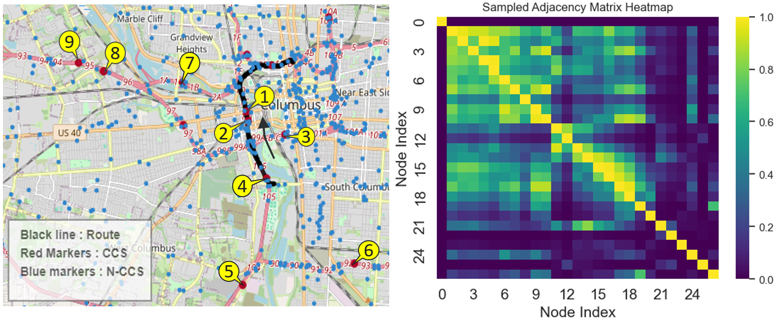
Figure 1: Sampled Route (left); Heat Map of Adjacency Matrix (right)

IV-B Evaluation Metric and Baselines

To measure and evaluate the performance of different methods, Mean Absolute Errors (MAE), and Root Mean Squared Errors (RMSE) are adopted.

$$\text{MAE}=\frac{1}{N}\sum_{i=1}^{N}|\mathbf{F}_{i}-\hat{\mathbf{F}}_{i}|$$ (21)

$$\text{RMSE}=\sqrt{\frac{1}{N}\sum_{i=1}^{N}(\mathbf{F}_{i}-\hat{\mathbf{F}}_{i})^{2}}$$ (22)

We compare our method with the following baselines:

• Spatio-Temporal Graph Convolutional Networks (STGCN): Combines graph and temporal convolutions for traffic prediction.

• Auto-Regressive Integrated Moving Average (ARIMA): Uses past values in a time series for prediction.

• Historical Average (HA): Predicts based on the average of past traffic data.

• Feed-Forward Neural Network (FNN): Basic neural network without temporal dependencies.

• Long Short-Term Memory (LSTM): Captures long-term dependencies in time-series data.

We also report mean prediction interval width (MPIW) and prediction interval coverage probability (PICP) to quantify uncertainty.

$$\text{PICP}=\frac{1}{N}\sum_{i=1}^{N}\mathbf{1}(\hat{\mathbf{F}}_{i}^{L}\leq\mathbf{F}_{i}\leq\hat{\mathbf{F}}_{i}^{U})$$ (23)

$$\text{MPIW}=\frac{1}{N}\sum_{i=1}^{N}(\hat{\mathbf{F}}_{i}^{U}-\hat{\mathbf{F}}_{i}^{L})$$ (24)

where $\hat{\mathbf{F}}_{i}^{L}$ and $\hat{\mathbf{F}}_{i}^{U}$ are the lower and upper bounds of the prediction interval for the $i$-th observation, respectively.

IV-C Results

Table I demonstrates the results for our model and comparison with the baselines on the ODOT-TCDS dataset. Our proposed model shows a reduction of 24% in MAE and 8% in RMSE compared with STGCN.

TABLE I: Comparison of MAE and RMSE across different models.

Method	ODOT-TCDS sub-sample (15 min)
	MAE	RMSE
STGCN	0.29	0.38
ARIMA	0.67	1.08
HA	0.51	0.75
FNN	0.39	0.53
LSTM	0.34	0.49
Proposed Model	0.22	0.35

Figure 2 illustrates the loss and MAE over epochs for the training and validation sets. The plots suggest that our model can achieve an acceptable convergence.

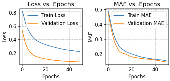
Figure 2: Loss versus Epochs (left); MAE versus Epochs (right)

The results for uncertainty quantification for a selected CCS node are shown in Figure 3. We used a forecast horizon of 15 min with a 24 hours of look-back period. It also shows the associated prediction intervals on actual flow data.

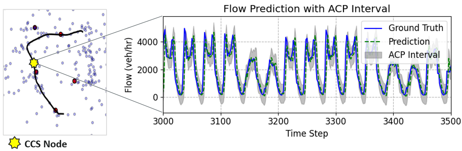
Figure 3: Prediction with Uncertainty Bounds

The proposed methodology for quantifying uncertainty showed a PICP of 90.02% and an MPIW of 1.03 which conveys that the resulting coverage probability falls within the expectation of 90% coverage rate as considered in ACP.

IV-D Traffic Model Calibration and Validation

We used the routesampler tool in SUMO to create a traffic scenario following the methodology in [29] for validation. We took the average values from the upper bound predicted by ACP to mimic a peak-hour scenario for morning hours of weekdays from 7:30 am to 8:30 am. Then, we conducted a Monte-Carlo simulation by varying the departure time of the generated vehicles for 200 runs and measured the VUT travel time parameter to evaluate the model’s performance which was compared against the INRIX probe data [31]. The results are shown in Figure 4.

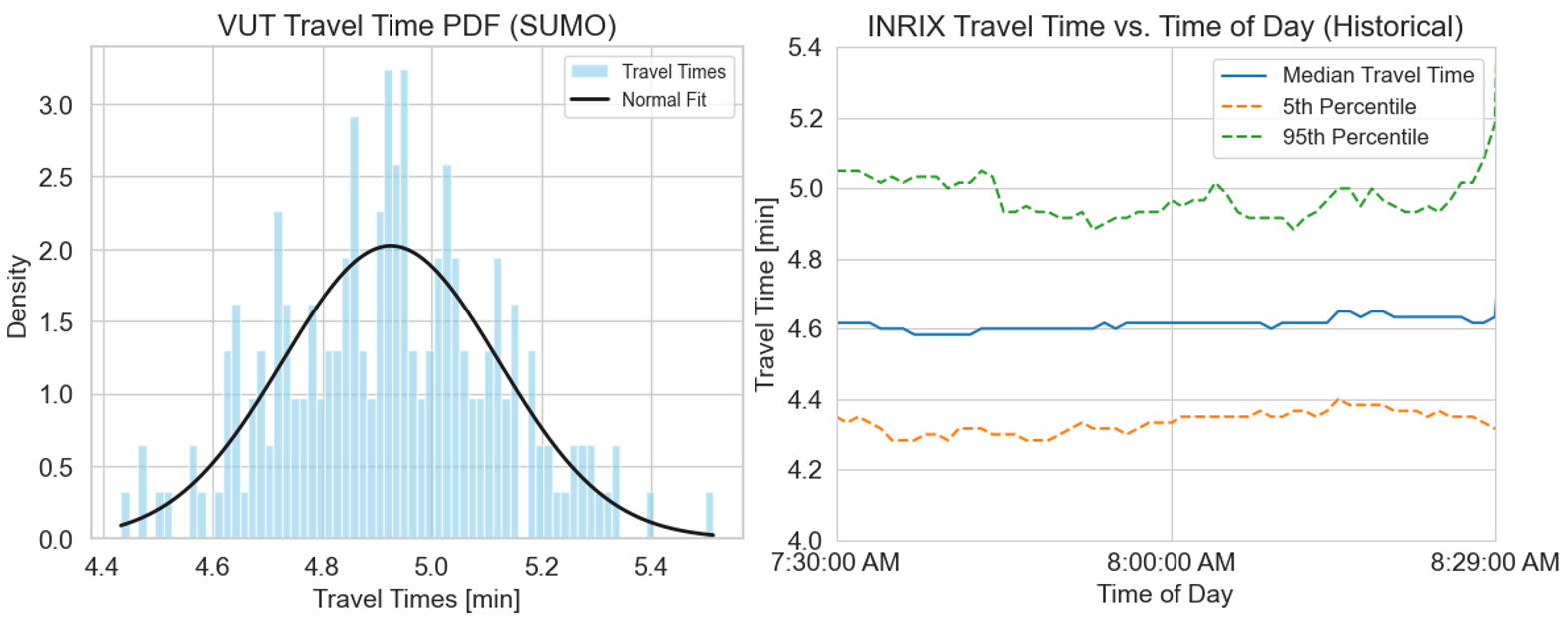
Figure 4: PDF of VUT travel times from Monte-Carlo SUMO simulations (left); INRIX Probe Data (right) during 7:30AM - 8:30AM

While discrepancies were present, as is expected in any model trying to mimic complex real-world phenomena, the overall trend of travel times during the selected period was captured reasonably well by the simulation. The distribution mean is around 4.93 minutes which is close to the 95th percentile from the INRIX probe data.

V CONCLUSIONS

In this study, we propose an approach that uses travel times to define the weights in a GNN’s adjacency matrix, simplifying it while maintaining a physics-like perspective. We also include data from all types of traffic monitoring stations for comprehensive coverage. To address uncertainty, we apply ACP method for better reliability. Finally, we validate the predictions through Monte-Carlo simulation in SUMO, assessing VUT travel time distribution against INRIX data, which showed that the predicted travel times closely matched the actual data.

In order to improve the model’s forecasting ability, future directions for this work will include a variety of urban contexts and the addition of outside variables like traffic accidents and weather fluctuations.

References

- [1] B. Pishue, ”2022 INRIX Global Traffic Scorecard,” Transportation Analyst, Jan. 2023.
- [2] B. Yu, H. Yin, and Z. Zhu, ”Spatio-temporal graph convolutional networks: A deep learning framework for traffic forecasting,” arXiv preprint arXiv:1709.04875, 2017.
- [3] Y. Li, R. Yu, C. Shahabi, and Y. Liu, ”Diffusion convolutional recurrent neural network: Data-driven traffic forecasting,” arXiv preprint arXiv:1707.01926, 2017.
- [4] L. Zhao, Y. Song, C. Zhang, Y. Liu, P. Wang, T. Lin, et al., ”T-GCN: A temporal graph convolutional network for traffic prediction,” IEEE Transactions on Intelligent Transportation Systems, vol. 21, no. 9, pp. 3848-3858, 2019.
- [5] S. Guo, Y. Lin, N. Feng, C. Song, and H. Wan, ”Attention based spatial-temporal graph convolutional networks for traffic flow forecasting,” in Proceedings of the AAAI Conference on Artificial Intelligence, vol. 33, no. 01, pp. 922-929, July 2019.
- [6] Z. Wu, S. Pan, G. Long, J. Jiang, and C. Zhang, ”Graph WaveNet for deep spatial-temporal graph modeling,” arXiv preprint arXiv:1906.00121, 2019.
- [7] C. Zheng, X. Fan, C. Wang, and J. Qi, ”GMAN: A graph multi-attention network for traffic prediction,” in Proceedings of the AAAI Conference on Artificial Intelligence, vol. 34, no. 01, pp. 1234-1241, April 2020.
- [8] Z. Li, G. Xiong, Y. Tian, Y. Lv, Y. Chen, P. Hui, and X. Su, ”A multi-stream feature fusion approach for traffic prediction,” IEEE Transactions on Intelligent Transportation Systems, vol. 23, no. 2, pp. 1456-1466, 2020.
- [9] Z. Cui, K. Henrickson, R. Ke, and Y. Wang, ”Traffic graph convolutional recurrent neural network: A deep learning framework for network-scale traffic learning and forecasting,” IEEE Transactions on Intelligent Transportation Systems, vol. 21, no. 11, pp. 4883-4894, 2019.
- [10] Z. Pan, Y. Liang, W. Wang, Y. Yu, Y. Zheng, and J. Zhang, ”Urban traffic prediction from spatio-temporal data using deep meta learning,” in Proceedings of the 25th ACM SIGKDD International Conference on Knowledge Discovery & Data Mining, pp. 1720-1730, July 2019.
- [11] K. Guo, Y. Hu, Z. Qian, Y. Sun, J. Gao, and B. Yin, ”Dynamic graph convolution network for traffic forecasting based on latent network of Laplace matrix estimation,” IEEE Transactions on Intelligent Transportation Systems, vol. 23, no. 2, pp. 1009-1018, 2020.
- [12] Y. Shin and Y. Yoon, ”Incorporating dynamicity of transportation network with multi-weight traffic graph convolutional network for traffic forecasting,” IEEE Transactions on Intelligent Transportation Systems, vol. 23, no. 3, pp. 2082-2092, 2020.
- [13] Q. Zhang, J. Chang, G. Meng, S. Xiang, and C. Pan, ”Spatio-temporal graph structure learning for traffic forecasting,” in Proceedings of the AAAI Conference on Artificial Intelligence, vol. 34, no. 01, pp. 1177-1185, April 2020.
- [14] L. Chen, W. Shao, M. Lv, W. Chen, Y. Zhang, and C. Yang, ”AARGNN: An attentive attributed recurrent graph neural network for traffic flow prediction considering multiple dynamic factors,” IEEE Transactions on Intelligent Transportation Systems, vol. 23, no. 10, pp. 17201-17211, 2022.
- [15] H. Yang, X. Zhang, Z. Li, and J. Cui, ”Region-level traffic prediction based on temporal multi-spatial dependence graph convolutional network from GPS data,” Remote Sensing, vol. 14, no. 2, art. 303, 2022.
- [16] B. D. Greenshields, ”A Study of Traffic Capacity,” Highway Research Board Proceedings, vol. 14, pp. 448-477, 1935.
- [17] M. J. Lighthill and G. B. Whitham, ”On Kinematic Waves II. A Theory of Traffic Flow on Long Crowded Roads,” in Proceedings of the Royal Society of London. Series A, Mathematical and Physical Sciences, vol. 229, pp. 317-345, 1955.
- [18] H. J. Payne, ”Models of Freeway Traffic and Control,” in Simulation Councils: Mathematical Models of Public Systems, 1971.
- [19] A. A. T. M. Aw and M. Rascle, ”Resurrection of ’Second Order’ Models of Traffic Flow,” SIAM Journal on Applied Mathematics, vol. 60, pp. 916-938, 2000.
- [20] M. Usama, R. Ma, J. Hart, and M. Wojcik, ”Physics-Informed Neural Networks (PINNs)-Based Traffic State Estimation: An Application to Traffic Network,” Algorithms, vol. 15, no. 12, art. 447, 2022.
- [21] J. Ji, J. Wang, Z. Jiang, J. Jiang, and H. Zhang, ”STDEN: Towards physics-guided neural networks for traffic flow prediction,” in Proceedings of the AAAI Conference on Artificial Intelligence, vol. 36, no. 4, pp. 4048-4056, June 2022.
- [22] Y. Wu and J. Q. James, ”A Bayesian learning network for traffic speed forecasting with uncertainty quantification,” in 2021 International Joint Conference on Neural Networks (IJCNN), pp. 1-7, IEEE, July 2021.
- [23] A. J. Khattak, J. Liu, B. Wali, X. Li, and M. Ng, ”Modeling traffic incident duration using quantile regression,” Transportation Research Record, vol. 2554, no. 1, pp. 139-148, 2016.
- [24] B. Lakshminarayanan, A. Pritzel, and C. Blundell, ”Simple and scalable predictive uncertainty estimation using deep ensembles,” in Advances in Neural Information Processing Systems, vol. 30, 2017.
- [25] K. Stankeviciute, A. M. Alaa, and M. van der Schaar, ”Conformal time-series forecasting,” in Advances in Neural Information Processing Systems, vol. 34, pp. 6216-6228, 2021.
- [26] K. Stankeviciute, A. M. Alaa, and M. van der Schaar, ”Conformal time-series forecasting,” in Advances in Neural Information Processing Systems, vol. 34, pp. 6216-6228, 2021.
- [27] J. Lin, J. Ma, J. Zhu, and Y. Cui, ”Short-term load forecasting based on LSTM networks considering attention mechanism,” International Journal of Electrical Power & Energy Systems, vol. 137, art. 107818, 2022.
- [28] B. M. Williams and L. A. Hoel, ”Modeling and forecasting vehicular traffic flow as a seasonal ARIMA process: Theoretical basis and empirical results,” Journal of Transportation Engineering, vol. 129, no. 6, pp. 664-672, 2003.
- [29] M. Patil, P. Tulpule, and S. Midlam-Mohler, ”An Approach to Model a Traffic Environment by Addressing Sparsity in Vehicle Count Data,” SAE Technical Paper No. 2023-01-0854, 2023.
- [30] M. Treiber, A. Hennecke, and D. Helbing, ”Congested traffic states in empirical observations and microscopic simulations,” Physical Review E, vol. 62, no. 2, pp. 1805, 2000.
- [31] INRIX, ”Roadway Analytics,” INRIX, 2020. [Online]. Available: https://inrix.com/products/roadway-analytics/. [Accessed: 11-Dec-2023].