Cosmological constraints on dynamical dark energy model in gravity
Abstract
Extended teleparallel gravity, characterized by function where is the non-metricity scalar, is one of the most promising approaches to general relativity. In this paper, we reexamine a specific dynamical dark energy model, which is indistinguishable from the CDM model at present time and exhibits a special event in the future, within gravity. To constrain the free parameters of the model, we perform a Markov Chain Monte Carlo (MCMC) analysis, using the last data from Pantheon+ and the latest measurements of the H(z) parameter combined. On the basis of this analysis, we have find that our dynamical dark energy model, in the context of F(Q) gravity, lies in the quintessence regime rather than in the phantom regime as in the case of general relativity. Furthermore, this behaviour affects the future expansion of the Universe as it becomes decelerating at confidence level for and showing a bounce at . Finally, we have support our conclusion with a cosmographic analysis.
I introduction
The study of the accelerated expansion of the Universe in the late-time is one of the most interesting areas of modern cosmology. This phenomenon has been confirmed and supported by different cosmological observations, namely the Supernovae Type Ia (SNIa) measurements perlmutter1999measurements ; riess1998observational , cosmic microwave background CMB1 ; CMB2 , baryon acoustic oscillations BAO1 ; BAO2 and large scale structure LS1 ; LS2 . To explain the acceleration phase of the Universe, an exotic negative-pressure component, dubbed dark energy (DE) is added to the Universe’s energy budget in the context of general relativity. Dark energy causes repulsive gravity behavior on large cosmological scales, initially described by the cosmological constant, einstein1917kosmologische with an equation of state (EoS) parameter, . This model, called Lambda Cold Dark Matter (CDM), is the most accepted by recent observational data 1A ; 2A ; 3A . Unfortunately, the CDM model has some serious theoretical problems, including fine-tuning RevModPhys.61.1 ; Peebles_2003 ; fin and coincidence problem con1 ; con2 in addition to various observation issues, called cosmological tensions T1 ; T2 ; T3 .
Several dynamical dark energy models have been proposed in order to overcome these problems, such as the quintessence martin2008quintessence ; chiba2000kinetically , k-essence armendariz2001essentials ; chimento2004power ; malquarti2003new , Chaplygin Gas kamenshchik2001alternative ; zhang2006interacting , holographic dark energy bouhmadi2018more ; li2004model ; belkacemi2020interacting ; belkacemi2012holographic ; bargach2021dynamical , generalized holographic dark energy granda2008infrared ; bouhmadi2011cosmology ; belkacemi2012holographic ; bouhmadi2018more and phantom dark energy where the EoS parameter is slightly less than ph ; dahmani2023constraining ; R1 . Phantom DE models have some drawback features as their energy density increases with the scale factor and becomes infinite at some point in the future and leads the Universe to end in a Big Rip singularity ph . Among the models proposed to cure this drawback, we cite the Little Sibling of the Big Rip (LSBR), which has been proposed as one of the mildest models of the possible apocalypse and describes perfectly the current acceleration of the Universe bouhmadi2015little . Several works have studied this model in cosmology LSBRH and in quantum cosmology LSBR5 ; LSBR8 (see also LSBR3 ; LSBR4 ; LSBR6 ; LSBR7 ). Moreover, it has recently been shown that this model is well supported by cosmological observations data amine , and can reduce the Hubble tension compared to the CDM model safae .
Another way of explaining this late acceleration is to modify the structure of the Einstein-Hilbert gravitational Lagrangian itself by considering scalar tensor theories Amendola1999 ; errahmani2006high or by replacing the Ricci scalar with a single-variable SV , two-variable TTV ; Errahmani:2024ran or even three-variable TV , where is the Ricci scalar, is the trace of the energy-momentum tensor and is the Kretschmann scalar. These approaches have led to many important extensions of general relativity, including gravity starobinsky1987new , gravity de2009construction , where G is the Gauss–Bonnet term, gravity erices2019cosmology , Horndeski scalar-tensor theories deffayet2009covariant etc. However, from a general differential geometric point of view, and taking into account the affine properties of manifolds, the curvature is not the only geometric object that may be used within a geometrical framework to construct gravitational theories. Indeed, torsion and non-metricity are two other essential geometric objects connected to a metric space, along with the curvature. They can be used to obtain bamba2013effective and nester1998symmetric ; jimenez2018coincident ; mandal2023cosmological gravity theories, where and are the torsion and the non-metricity scalar, respectively.
Recently, many different applications of gravity have been studied. Among these, the authors of lazkoz2019observational , have found an interesting result for the current value of the Hubble parameter, which was close to the Planck’s estimate, by considering the Lagrangian as a polynomial function of redshift. To demonstrate the late-time acceleration of the Universe, a new parametrization of the EoS parameter in the context of , was established in koussour2023observational .
Thanks to the energy conditions, the authors of mandal2020energy have restricted the families of models compatible with the accelerated expansion of the Universe. A new class of theories, in which the non-metricity scalar is coupled non-minimally to matter Lagrangian has been proposed by harko2018coupling , where the cosmological solutions are considered in two general classes of models, and are characterized by the accelerated expansion at late time. In addition, the authors of MhamdiEPJC2024 have shown that the model is well supported by the background and perturbation data, using a particular form of . For more studies related to the applications of gravity see for instance mandal2023cosmological ; cosmology ; anagnostopoulos2021first ; anagnostopoulos2023new ; mandal2022reply ; khyllep2021cosmological ; beh2022geodesic ; MhamdiEPJC2024 .
In this paper, we aim to reexamine the current accelerated expansion of the Universe by considering the specific dynamical dark energy (DDE) model bouhmadi2015little , in the context of gravity. Indeed, in the context of general relativity, this kind of dark energy mimics a phantom like behaviour and smooth the big rip singularity in a good agreement with the observational data dahmani2023constraining ; LSBR3 ; amine ; safae . Furthermore, This dark energy model predicts more dark matter in the past safae and reproduces CDM in the current time. As we will show, some of these properties will undergo a change in the context of gravity R2 ; R3 ; R4 . Among these: this dark energy will behave as a quintessence, the expansion will decelerates and the Universe will faces a bounce in the future.
In this line, we estimate constraints of the cosmological parameters of our setup. We first perform cosmological analysis with Markov Chain Monte Carlo (MCMC) approach MCMC , using the most recent data from Supernovae type Ia, namely Pantheon+ Pan combined with data 7 . We then perform a statistical comparison between our model and CDM by using the Akaike Information Criterion (AIC) akaike1974new ; AIC and the Bayesian Information Criterion (BIC) BIC . In addition, we present a cosmographic analysis of the model, including the evolution of the deceleration parameter (q), jerk parameter (j), and snap (s) parameter 1 ; 2 ; 3 .
The outline of this article is as follows: In Section II, we give a brief review of the gravity, in Section III, we present the modified Friedman equations in the gravity. In Section IV, we describe the methodology of the datasets. In Section V we present the results and discussions. Section VI is devoted to the cosmographic analysis of the model. Finally, in Section VII we summarize our results.
II Overview of gravity
In this section, we give a brief introduction to the formalism of gravity. We consider modified gravity, in which the basic object is the non-metricity tensor , given by nester1998symmetric
| (1) |
The non-metricity scalar, which is an important quantity in this theory, is defined in terms of the disformation tensor, , as follows
| (2) |
where the disformation tensor is symmetrical with respect to lower indices and is defined by
| (3) |
In terms of the non-metricity conjugate, the non-metricity scalar is given by
| (4) |
where the non-metricity conjugate, , is defined in terms of the non-metricity tensor and its two independent traces, and , as
| (5) |
The action of the modified gravity is written as follows jimenez2018coincident
| (6) |
where is a function of the non-metricity scalar , g is the determinant of the metric and is the Lagrangian density of matter. The field equation of the gravity is obtained by varying the action with respect to , and it takes the following form
| (7) |
where , and the energy-momentum tensor, , is given by
| (8) |
By varying the action with respect to the affine connection mandal2023cosmological , we obtain the following equation
| (9) |
III cosmological model
To examine the cosmological consequences of the gravity, we consider the Friedmann-Lemaître-Robertson-Walker (FLRW) line element, which describes the flat, homogeneous, and isotropic Universe, is given by
| (10) |
where is the cosmic time, , and denote the Cartesian coordinates, is the cosmic scale factor, and the Hubble parameter is defined by , with denotes the derivative of the scale factor with respect to the cosmic time.
III.1 The generalized Friedmann equations
In the FLRW geometry, we get the non-metricity scalar as . We consider the matter content of the Universe as consisting of a perfect and isotropic fluid, with the energy momentum tensor given by
| (11) |
where and are the pressure and the energy density of the fluid, respectively, is the four velocity vector normalized according to
.
To better fulfill our goal, we consider the splitting of as . Using the FLRW metric, we get two Friedmann equations as jimenez2018coincident ; cosmology
| (12) | |||||
| (13) |
where we have set . According to the above equations, we recover the standard model, for (i.e. ). The same equations, Eqs. (12) and (13) can be rewritten as
| (14) |
where we have introduced a geometrical dark energy density, , and its pressure, , as follows
| (15) |
Furthermore, the effective equation of state using Eq. (14) can be written as,
| (16) |
III.2 Dynamical dark energy
In order to understand the characteristic properties of the dark energy driving the recent acceleration of the Universe, we need to parameterize its equation of state (EoS). To this aim, we consider one of the main studied dynamical dark energy given by bouhmadi2015little
| (17) |
where , , and are the energy density, the pressure, and a constant characterizing the dark energy model, respectively.
The primary motivation for taking into account this parametrization form is its advantage to smooth the big rip singularity. Indeed, in this scenario, the size of the observable Universe and its expansion rate grow to infinity while the cosmic time derivative of the Hubble parameter converges to a constant value. Furthermore, this model deviates slowly from the standard model, by the constant and it behaves as phantom like dark energy models. The equation of state of this dynamical dark energy model, dubbed Little Sibling of the Big Rip (LSBR) in bouhmadi2015little , is given by
| (18) |
according to Eq. (18), the DDE model describes a phantom DE, for positive values of (i.e. ). For negative values of , the model describes a quintessence DE (i.e. ) and mimics the standard model in the limit . Despite the aforementioned advantages, The DDE model faces some drawbacks. Indeed, This dynamical dark energy model is unable to describe the very early expansion of the Universe as its energy density becomes negative i.e. it is not supported by high redshifts safae .
Using Eqs. (15) and (17), we get
| (19) |
the dot (.) indicates the derivative with respect to cosmic time. Using the relation between the derivative of and the non-metricity scalar
| (20) |
where , Eq. (19) becomes
| (21) |
In order to illustrate our purpose, we consider the following form of mandal2023cosmological
| (22) |
where , and are constants. In this case, Eq. (21) becomes
| (23) |
we also can write this equation in the form
| (24) |
By integration, we obtain
| (25) |
Combining Eqs (22) and (15) gives the form of in terms of as
| (26) |
which in terms of , it becomes
| (27) |
We finally obtain the Friedmann equation, from Eq. (14), as follows
| (28) |
where is the dimensionless Hubble rate, and and we have used .
The last two terms in Eq. (28) represent the dimensionless parameters of dark energy density, which can be expressed as
| (29) |
From Eq. (28), the model predicts an increase in dark matter density as . However, in the future, the model is dominated by dark energy, and its behavior is characterized by the sign of . Eq. (28) can be approximated as follows: . For being positive, the Hubble rate diverges while its derivative remains constant bouhmadi2015little . This abrupt event, termed ”Little Sibling of the Big Rip”, smooths the big rip singularity in the future. This phenomenon has been extensively studied in references safae ; bouhmadi2015little ; LSBR5 ; LSBR8 . However, if is negative, the Universe’s dynamical behavior undergoes a bounce, as we will illustrate in section V. From now on, we will refer to our setup as -DDE.
IV Statistical analysis
In order to obtain optimal constraints on cosmological parameters of the -DDE model and compare them with those of the CDM model, we perform a Markov Chain Monte Carlo (MCMC) analysis, using the last data from Pantheon+ and Hubble parameter data (H(z)). We consider a parameter space composed of the Hubble constant, , the density parameter of total matter, , the two parameters that describe the gravity, , and , as well as the DDE parameter, , by means of the dimensionless parameter, . The prior related to the free parameters is given in Tab. (1)
| Parameters | Prior |
|---|---|
| [] | |
| [] | |
| [] | |
| [] | |
| [] | |
| [] |
IV.1 Pantheon+ dataset
We use the latest Pantheon+ measurements Pan , composed of 1701 light curves of 1550 distinct Supernovae Type Ia (SNIa) confirmed by spectroscopy, ranging in interval, .
The function is written as
| (30) |
where is the covariance matrix and is a vector where each of its elements refers to the distance modulus of SNIa, given by
| (31) |
where is the distance modulus for the Cepheid calibrated host-galaxy of the SNIa provided by SH0ES SH0ES and is the theoretical distance modulus, defined as
| (32) |
where is the absolute magnitude, is the apparent magnitude and is the luminosity distance, defined as
| (33) |
is the speed of light.
IV.2 H(z) Data
Secondly, we use Hubble expansion rate data 7 to impose tighter constraints on our F(Q)-DDE model. Generally, data can be obtained either through the clustering of galaxies and quasars, measured via Baryon Acoustic Oscillations (BAO) in the radial direction data2 , or through the differential age method data3 . In our current analysis, we have employed a compilation of 36 data points of the Hubble parameter, which exhibit no correlation. The function is given by
| (34) |
where is the theoretical values, is the observed values at and is the standard deviation.
To analyze both the H(z) data and type Ia supernovae samples simultaneously, we use the total Chi-square function given by
| (35) |
IV.3 Information criteria
The aim of this work, besides the parameter estimations, is to select the best model supported by the observation data. In fact, a model with a smaller value of indicates that the model is well fitted to the observation data. However, a large number of parameters can increase the quality of the fit and therefore lead to a smaller . In this case, the statistics is not an appropriate way to compare models. To confidently predict the goodness of the fit between the -DDE and CDM models, we use another statistical tool, namely the Akaike Information Criterion (AIC) akaike1974new ; AIC , which depends on the number of parameters, , given by
| (36) |
As statistics, a model with a smaller value of AIC indicates that the model is most supported by the observation data. For this we calculate111In our analysis, we have considered the CDM model as a reference model.
| (37) |
The model selection rule of AIC, is as follows: for 0AIC2, it suggests that the model has nearly the same level of support from the observation data as CDM, for 2AIC4, it indicates the model has slightly less support compared to the CDM model, for 4AIC10 the data still support the model but less than the preferred one and for , the model is not supported by the observational data compared to the CDM model.
We also calculate the Bayesian information criterion (BIC), given by BIC
| (38) |
where a smaller value of BIC indicates that the model is most supported by the observation data. For this we calculate
| (39) |
A positive (negative) value of BIC shows that the -DDE (CDM) model is preferred. The selection rules of BIC is as follows: for 0BIC2 means that the evidence is insufficient, for 2BIC6, indicates that there is a positive evidence while for BIC indicates a solid evidence.
V Results and discussions
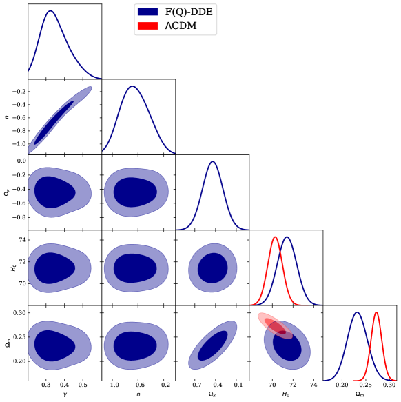
In Table (3), we present the 68% C.L. constraints on the cosmological parameters of the CDM and -DDE models obtained using combination of Pantheon+ and H(z) data. Fig. (1) shows the 1D posteriori distributions and 2D marginalized contours at and for the CDM and -DDE models. From Table (3), the Hubble constant values are km/s/Mpc for the -DDE model and km/s/Mpc for CDM at 68% C.L.. The latter is smaller, at around from the value obtained by -DDE. In Table (3), we also list constraints on the two parameters describing the gravity, i.e. (, )=( , ). We observe a strong correlation between these two parameters in Fig. (1). Furthermore, we notice that in the -DDE gravity, the DDE parameter value is negative i.e. at 68% C.L., which from Eq. (18) leads to . This shows that, in the context of gravity, the DDE model behaves like a quintessence one, contrary to the results found in bouhmadi2015little ; LSBR3 ; amine ; safae where it is shown that observational data prefer the phantom like behaviours of DDE.
Moreover, the future evolution of the Universe depends strongly on the sign of , and . Indeed, in the future (i.e. ), the asymptotic behavior of the Friedmann equation (28) can be simplified to
| (40) |
and is an increasing function of . This means that decreases as the Universe expands and, consequently, the Universe will bounce (i.e. ) at some point in the future where the redshift can be approximated to . Using the numerical values, from Table (3), for , and , the redshift corresponding to the bounce can be estimated to . This scenario can be interpreted as follow: the dark energy density, described by Eq. 27 and which drives the current accelerated expansion of the Universe, decreases as the Universe expands. At this point, the Universe undergoes a bounce and starts contracting. While in the context of general relativity, this dark energy density smooths the big rip singularity.
In the same table, we present the value of , AIC as well as BIC. According to the value, we see that the DDE model in the context of gravity increases the goodness of fit to the observational data over CDM, with . However, a large number of parameters can lead to a smaller value of and thus increase the quality of the fit. To confidently predict the goodness of fit between models, we use the Akaike Information Criterion (AIC) and Bayesian information criterion (BIC), which depend on the number of parameters. According to Tab. 3, we obtain , which gives a statistical preference for our model. However, the positive sign of shows a preference for the CDM model over our model as this criterion penalizes models with additional parameters.
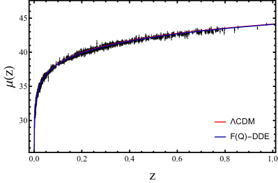
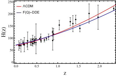
Fig. (2) shows the theoretical evolution of the distance modulus (left panel) and the Hubble function (right panel), predicted by the F(Q)-DDE model as a function of , using the results presented in Table (3). For comparison, both data samples are also presented in the same figure according to the theoretical prediction of the CDM model. This figure shows that the F(Q)-DDE model behaves identically to CDM, and that both models are in good agreement with the observational data.
| Parameters | CDM | -DDE |
| - | ||
| - | ||
| - | ||
| statistical results | ||
| AIC | ||
| AIC | ||
| BIC | ||
| BIC | ||
VI Cosmographic analysis
VI.1 Cosmographic parameters
Given the large number of cosmological models that have been proposed to explain the late accelerated expansion of the Universe,
a mathematical tool, without assuming a dark energy models, is useful to discriminate between all proposed dark energy models. An approach called cosmography has been proposed for this reason COS ; COS1 ; COS2 . This analysis makes it possible to compare several cosmological models using the derivatives of scale factor by means of the Taylor series expansion of the scale factor 3 ; H1 ; H2 .
The aim of this part is to study the Taylor series expansion of the scale factor with respect to cosmic time, , by introducing the following cosmographic parameters: the Hubble parameter, deceleration parameter, jerk parameter and snap parameter, defined respectively as follows
| (41) |
| (42) |
| (43) |
| (44) |
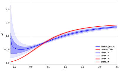
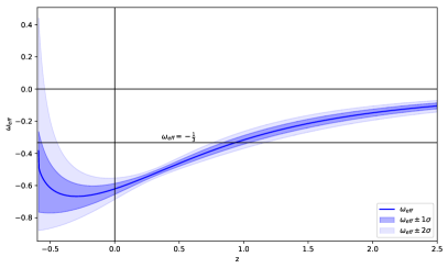
Fig. 3, shows the evolution of the mean value of the deceleration parameter and its uncertainty at 1 and 2 as a function of redshift for the -DDE and CDM models (left panel) and the evolution of for the -DDE model (right panel). The parameter measures the rate at which the expansion of the Universe is accelerating or decelerating. In particular, positive values of indicates that the expansion is decelerating, which also corresponds to , while negative values of indicate that the expansion is accelerating and . Fig. (3) shows that the expansion of the Universe is characterized by a transition phase, from deceleration to acceleration in the recent past. For our model, the phase transition (i.e. ) occurs at redshift , while the redshift transition for CDM is less than that of -DDE, i.e. at . For our model, we obtain the actual value of the deceleration parameter, , with a difference of compared to the CDM model, where . The most important result in Fig. (3) is that a phase transition in the future from accelerating to decelerating expansion at the confidence level, in the redshift , is possible. This result is also confirmed by the equation of state, , where at in the redshift (see the right panel of Fig. (3)). This conclusion is recently found in futur . We also note that and that the model is in the quintessence region for all redshifts.
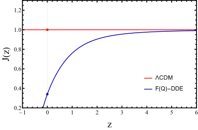
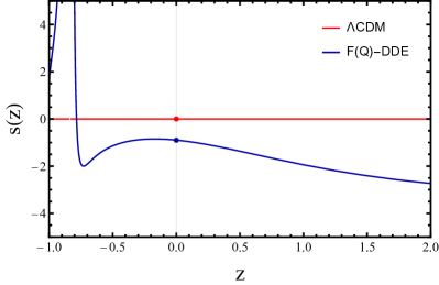
Fig. 4, shows the evolution of the jerk parameter (left panel) and the snap parameter (right panel) as functions of the redshift. The red and blue points represent the present time (), for the CDM and F(Q)-DEE models, respectively. The left panel of Fig. 4 shows that the jerk parameter approaches unity, in the near past (i.e. ). Therefore, our model behaves identically to the CDM, as the jerk parameter always remains constant, . At the present time, we obtain a positive value of the jerk parameter with a difference of compared to the CDM model and we can see a significant deviation between -DDE and CDM for low and negative redshifts (see the left panel of Fig. 3). The right panel of Fig. 4 shows the evolution of the snap parameter. From this figure, we notice significant deviations between -DDE and CDM for all redshifts. The present value of the snap parameter for our model is with a difference of compared to the CDM model.
| Parameters | CDM | -DDE |
|---|---|---|
VI.2 Statefinder diagnostic
In this section, we use statefinder diagnostic technique which is an alternative tools to compare and distinguish between different models of dark energy ST ; ST1 . This geometric technique uses the pair of parameters , where is the jerk parameter and is snap parameter, defined as follows ST ; ST1
| (45) |
| (46) |
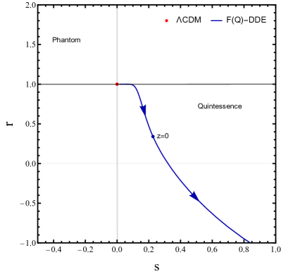
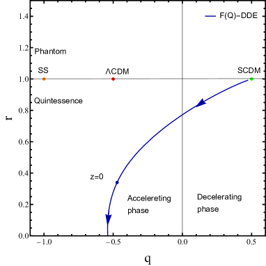
In order to evaluate the behavior of our model, the trajectories of the pairs and are represented in Fig. 5, where the arrows represent the time evolution from the past to the future. The left panel of Fig. 5 displays the evolutionary trajectory of the plane. From this figure, our model is located in the quintessence region (i.e. and ). The right panel of Fig 5 shows the evolutionary trajectory of the plane. We notice that the evolution of our model starts from the region where the Universe is dominated by matter abbreviated by SCDM ( and ), and converges to a point (, ), representing the late-time evolution of the Universe.
VII Conclusions
In this study, we reevaluate the dynamical dark energy (DDE) model in gravity. This dark energy model has been previously studied in the context of general relativity, exhibiting phantom behavior bouhmadi2015little . The model predicts more dark matter density in the past. However, in the future, the model is dominated by dark energy and exhibits distinctive behavior depending on the sign of . Specifically, for a positive value of , this abrupt event is dubbed ”Little Sibling of the Big Rip”, as it smooths the big rip singularity. Conversely, this event leads the Universe to bounce when is negative.
To understand the nature of the DDE model within gravity, we constrained the model parameters by performing a Markov Chain Monte Carlo analysis using a combination of two different background datasets, namely the Pantheon+ and Hubble parameter data. We have found that for the CDM model, and . However, for the -DDE model, , , , and . In particular, we obtained a negative value for the DDE parameter, at 68% C.L., indicating that the DDE model in F(Q) gravity is strictly oriented towards a quintessence region, and in the future the Universe bounce.
In addition, we have obtained , indicating that the model fits the observational data well.
However, relying solely on to compare models with different numbers of free parameters is not enough. Therefore, we also evaluated the AIC and BIC values. Our findings show that -DDE model is slightly more preferable in terms of AIC compared to CDM where AIC = -6.76. Conversely, our model is less favored in terms of BIC, where BIC = +4.16 in favor of CDM. Additionally, the theoretical predictions of the distance modulus and the Hubble function from the -DDE model are in good agreement with both data samples.
Unlike the case in the context of general relativity, we have noticed that our setup in the context of gravity behaves as like a quintessence and faces a bounce in the future at . We have found that the phase transition from deceleration to acceleration, in -DDE, stars late than CDM. We have also evaluated the current cosmographic parameters including deceleration parameter , jerk parameter , and snap parameter . Finally, we have analyzed the statefinder diagnostics in the and planes. We have found that, from statefinder diagnostic , our model is located in the quintessence region while from the plane, the DDE model evolves from a state where the Universe is dominated by matter in the past to a late-time state of the Universe.
References
- (1) S. Perlmutter et al., The Astrophysical Journal 517, 565 (1999).
- (2) A. G. Riess et al., The astronomical journal 116, 1009 (1998).
- (3) R.R. Caldwell, M. Doran, Phys. Rev. D 69, 103517 (2004).
- (4) Z.Y. Huang et al., JCAP 0605, 013 (2006).
- (5) D.J. Eisenstein et al., Astrophys. J 633, 560 (2005).
- (6) D.J. Eisenstein et al., MNRAS. 401, 2148 (2010).
- (7) T. Koivisto, D.F. Mota, Phys. Rev. D 73, 083502 (2006).
- (8) S.F. Daniel, Phys. Rev. D 77, 103513 (2008).
- (9) A. Einstein, Berlin, part 1, 142 (1917).
- (10) M. Blomqvist, et al., Astron. Astrophys. 629, A86 (2019).
- (11) Planck Collaboration: N. Aghanim et al., Astron. Astrophys. 641, A6 (2020).
- (12) T. M. C. Abbott et al., ApJL. 872, L30 (2019).
- (13) S. Weinberg, Rev. Mod. Phys. J. 61, 1-23 (1989).
- (14) P. J. E. Peebles, B. Ratra, Rev. Mod. Phys. 75, 559–606 (2003).
- (15) S. X. Tián, Phys. Rev. D 101, 063531 (2020).
- (16) H.E.S. Velten, R.F. vom Marttens, W. Zimdahl, Eur. Phys. J. C74 11, 3160 (2014).
- (17) N. Sivanandam, Phys. Rev. D 87, 083514 (2013).
- (18) L. Verde et al. Nature Astronomy 3, 891–895 (2019).
- (19) E. Di Valentino et al., Class. Quantum Grav. 38, 153001 (2021).
- (20) A. Elcio et al., J. High En. Astrophys 34, 49–211 (2022).
- (21) J. Martin, Modern Physics Letters A 23, 1252 (2008).
- (22) T. Chiba et al., Physical Review D 62, 023511 (2000).
- (23) C. Armendariz-Picon et al., Physical Review D 63, 103510 (2001).
- (24) L. P. Chimento et al., Modern Physics Letters A 19, 761 (2004).
- (25) M. Malquarti et al., Physical Review D 67, 123503 (2003).
- (26) A. Kamenshchik et al., Physics Letters B 511, 265 (2001).
- (27) H. Zhang et al., Physical Review D 73, 043518 (2006).
- (28) M. Bouhmadi-López et al., The European Physical Journal C 78, 1 (2018).
- (29) M. Li, Physics Letters B 603, 1 (2004).
- (30) Belkacemi, Moulay-Hicham et al., International Journal of Modern Physics D, 29, 2050066 (2020).
- (31) Belkacemi, Moulay-Hicham et al. Physical Review D, 85, 083503 (2012).
- (32) Bargach, Farida et al., International Journal of Modern Physics D, 30, 2150076 (2021).
- (33) L. Granda et al., Physics Letters B 669, 275 (2008).
- (34) Bouhmadi-López, Mariam et al., Physical Review D, 84, 083508 (2011).
- (35) R.R. Caldwell, Phys.Lett.B 545, 23-29 (2002).
- (36) S. Dahmani et al., General Relativity and Gravitation, 55, 22 (2023).
- (37) S. A. Narawade et al., arXiv: 2303.01985[gr-qc].
- (38) M. Bouhmadi-Lopez et al., Int. J. Mod. Phys. D 24, 1550078 (2015).
- (39) B. Vasilev et al., Phys. Rev. D 100, 084016 (2019).
- (40) I. Albarran et al., JCAP 11, 044 (2015).
- (41) M. Bouhmadi-López et al., JCAP 09, 031 (2018).
- (42) A. Bouali et al., Phys. Dark. Univ. 34, 100907 (2021).
- (43) I. Albarran et al., Phys. Dark. Univ. 16, 94-108 (2017).
- (44) J. Morais et al., Phys. Dark. Univ. 15, 7-30 (2017).
- (45) M. Bouhmadi-Lópezet al., JCAP 03, 042 (2017).
- (46) A. Bouali et al., Phys. Dark. Univ. 26, 100391 (2019).
- (47) S. Dahmani et al., Phys. Dark. Univ. 42, 101266 (2023).
- (48) L. Amendola, Phys. Rev. D 60, 043501 (1999).
- (49) A. Errahmani et al., Physics Letters B 641, 357 (2006).
- (50) S. Nojiri and S. D. Odintsov, Phys.Rept. 505, 144 (2011).
- (51) J. Rosa, Physical Review D 103, 104069 (2021).
- (52) A. Errahmani, et al., Phys. Dark Univ. 45, 101512 (2024).
- (53) M. Miranda et al., Eur. Phys. J. C . 81, 975 (2021).
- (54) A. A. Starobinsky, Quantum Cosmology 3, 130 (1987).
- (55) A. De Felice et al., Physics Letters B 675, 1 (2009).
- (56) C. Erices et al., Physical Review D 99, 123527 (2019).
- (57) C. Deffayet et al., Physical Review D 79, 084003 (2009).
- (58) K. Bamba et al., Physics Letters B 725, 368 (2013).
- (59) J. M. Nester et al., arXiv preprint gr-qc/9809049 (1998).
- (60) J. B. Jiménez et al., Physical Review D 98, 044048 (2018).
- (61) S. Mandal et al., The European Physical Journal C 83, 1141 (2023).
- (62) R. Lazkoz et al., Physical Review D 100, 104027 (2019).
- (63) M. Koussour et al., The European Physical Journal C 83, 400 (2023).
- (64) S. Mandal et al., Physical Review D 102, 024057 (2020).
- (65) T. Harko et al., Physical Review D 98, 084043 (2018).
- (66) D. Mhamdi et al., The European Physical Jounal C 84, 310 (2024).
- (67) J. B. Jiménez et al., Physical Review D 101, 103507 (2020).
- (68) F. K. Anagnostopoulos et al., Physics Letters B 822, 136634 (2021).
- (69) F. K. Anagnostopoulos et al., The European Physical Journal C 83, 1 (2023).
- (70) S. Mandal et al., Physical Review D 106, 048502 (2022).
- (71) W. Khyllep et al., Physical Review D 103, 103521 (2021).
- (72) J.-T. Beh et al., Chinese Journal of Physics 77, 1551 (2022).
- (73) S. A. Narawade and B. Mishra, Annalen der Physik, 535, 2200626, (2023).
- (74) S. A. Narawade et al., Physics of the Dark Universe, 42, 101282, (2023).
- (75) S. A. Narawade et al., Physics of the Dark Universe, 36, 101020, (2022).
- (76) L. E. Padilla et al., Universe 97, 213 (2021).
- (77) D. Brout et al, Astrophys . J. 938, 110 (2022).
- (78) Sharov G.S. and Vorontsova, J. Cosmol. Astropart. Phys, 10, 057 (2014).
- (79) H. Akaike, IEEE transactions on automatic control. 19, 716–723 (1974).
- (80) A. R. Liddle, MNRAS. 377, L74–L78 (2007).
- (81) G. Schwarz, Ann. Stat. 6, 461 (1978).
- (82) V. Sahni et al., J. Exp. Theor. Phys. 77, 201 (2003).
- (83) U. Alam et al., Mon. Notices Royal Astron. Soc. 344, 1057 (2003).
- (84) D. Mhamdi et al., Gen. Relativ. Gravit. 55, 11 (2023).
- (85) A. G. Riess et al., ApJ. L7 934, (2022).
- (86) J. E. Bautista et al., Astron. Astrophys. 603, A12 (2017).
- (87) S. Joan, Phys. Rev. D. 71, 255-262 (2005).
- (88) M. Visser, Classical Quantum Gravity, 21, 2603 (2004).
- (89) M. Visser, Gen. Relativ. Gravitation, 37, 1541 (2005).
- (90) M. Visser and C. Cattoen, Dark Matter In Astrophysics And Particle Physics. World Scientific, p. 287 (2010).
- (91) A. Bouali, et al., MNRAS 526 (3) (2023).
- (92) A. Bouali, et al., Fortschritte der Physik 71 (10-11), 2300033 (2023).
- (93) A. Lewis, arXiv:1910.13970 (2019).
- (94) Escobal, A. A., et al., Physical Review D 109.2, 023514 (2024).
- (95) V. Sahni et al., J. Exp. Theor. Phys. 77, 201 (2003).
- (96) U. Alam et al., Mon. Notices Royal Astron. Soc. 344, 1057 (2003).