Statistical mechanics of passive Brownian particles in a fluctuating harmonic trap

Abstract

We consider passive Brownian particles trapped in an "imperfect" harmonic trap. The trap is imperfect because it is randomly turned off and on, and as a result particles fail to equilibrate. In other words, the harmonic trap is time-dependent on account of its strength evolving stochastically in time. Particles in such a system are passive and activity arises through external control of a trapping potential, therefore, no internal energy is used to power particle motion. A stationary Fokker-Planck equation of this system can be represented as a third-order differential equation, and its solution, a stationary distribution, can be found by representing it as a superposition of Gaussian distributions for different strengths of a harmonic trap. The resulting stationary distributions tend to be spread out with an exponential asymptotic tail. A pure Gaussian distribution is recovered only in the limit of a very fast alternating on and off cycle. The average potential energy of the system is found to be the same as that for a system in equilibrium, that is, for a system with a time independent harmonic trap. The entropy production rate, which quantifies the distance from equilibrium, is found to be independent of the rate with which the trap fluctuates.

I Introduction

A typical active particle system consists of particles that derive motion from an internal energy source. Standard models that represent such particles are the run-and-tumble (RTP) Tailleur08 ; Tailleur09 ; Evans18 ; Dhar18 ; Dhar19 ; Basu20 ; Soto20 ; Razin20 ; Frydel21b ; Frydel21c ; Farago22 ; Frydel22b ; Connor23 ; Farago24 ; Ybert24 ; Loewe24 and active-Brownian particle (ABP) models Dhar20 ; Cargalio22 , one more suitable to biological and the other to chemical systems. Another active scenario arises when a passive Brownian particle is immersed in a bath of active particles. The model that addresses this situation is the active Ornstein-Uhlenbeck particle model (AOUP) Szamel14 ; Shankar18 ; Sevilla19 ; Cates21 ; Marconi18 ; Lowen22 .

A different and less explored design of active dynamics is realized by placing passive Brownian particles in a fluctuating external potential, thereby preventing particles from equilibrating. In this setup, there is no need for a special type of particles and the only requirement is that an external potential varies stochastically with time. A possible experimental realization of such a system could be attained using tweezer instruments and techniques Yael11 ; Brady16 ; Brady21 ; Lowen22b ; Genet22 ; Yael23 .

This work considers passive Brownian particles trapped in a harmonic potential $u=Kr^{2}/2$ with time-dependent strength $K\equiv K(t)$. We consider a specific evolution of $K(t)$ in which $K(t)$ changes discontinuously between two discrete values, zero and another finite value of the strength, therefore, the trap is either off or on. We refer to this external potential as "imperfect" harmonic trap. The trap fluctuations are implemented by random sampling of the times during which a potential is in a given state, $t_{p}$, from an exponential probability distribution $\sim e^{-t_{p}/\tau}$. This means that on average the the times during which a trap is on and off are the same and what changes is the rate, given by $\tau^{-1}$, with which the trap fluctuates between the two states.

A stationary situation of this system gives rise to a third-order differential equation. A third-order differential equation has previously been found to arise for run-and-tumble particles in a harmonic trap in one- and two-dimensions Frydel22c ; Frydel23b . The solution was found to be a convolution of two distributions, each one separately obeying a first-order differential equation. The convolution form of the solution reflects the fact that the two random processes involved, Brownian motion and active dynamics, remain independent in a harmonic potentia Frydel24a .

In the present system, a solution of the corresponding third-order equation can be represented as a superposition of Gaussian distributions for different strengths of a harmonic trap. This decomposes the solution into two contributions, a Gaussian distribution and the probability distribution of effective trap strengths, each distribution satisfying a first-order differential equation. The superposition of Gaussian distributions has been known in quantum theory and financial markets Kleinert04 ; Kleinert08 . In non-equilibrium statistical mechanics, those distributions have been considered in Beck01 in the context of non-extensive statistical mechanics.

The current work could be viewed as related to the systems that explore control of external forces and information feedback to perform work Sagawal15 ; Sagawa08 ; Cao09 ; Horowitz10 ; Sagawa10 ; Pon10 ; Suzuki10 ; Kundu12 . Although the model that is analyzed does not involve information feedback and the only control comes from regulating the time duration when particles are either trapped or released, it could be considered a small first step in theoretical understanding of this class of problems. In a more general context, by proposing a non-equilibrium model and solving it, the current work contributes an item to the collection of exactly solvable non-equilibrium problems.

This work is organized as follows. In Sec. (II) we introduce the model and obtain a third-order differential equation for a stationary state. In Sec. (III) we represent the solution as a superposition of Gaussian distributions for different trap strengths K. In Sec. (IV) we consider particles trapped in a harmonic potential with a general time-dependent trap strength. It is shown that the time-dependent distribution at any given moment is a Gaussian distribution. This result justifies the use of the superposition formula. In Sec. (V) we extend all the exact results to a system for an arbitrary dimension. In Sec. (VI) we consider quantities of physical interest. The work is concluded in Sec. (VII).

II The model

The focus of this work is a conceptually simple model: an ideal gas trapped in an "imperfect" harmonic potential. The potential is imperfect because it is turned off and on at random time intervals. The alternate cycle of trapping and releasing prevents particles from attaining equilibrium and as a result gives rise to a non-equilibrium situation. The times $t_{p}$ during which a particle is either trapped or released are sampled from the exponential distribution $\sim e^{-t_{p}/\tau}$, where $\tau$ is the average time during which a particle persists in a given state. At the end of each time $t_{p}$, a particle switches to another state with probability one.

Since the times when a trap is in the "on" and "off" state are sampled from the same distribution, the system spends on average the same amount of time in both states. What changes is the rate, given by $\tau^{-1}$, with which the trap fluctuates between the two states. The model represents a specific case of a harmonic potential $u=Kr^{2}/2$ with the time-dependent strength $K\equiv K(t)$.

For a system in one-dimension, the Fokker-Planck formulation that describes such a model might be written as

$$\dot{\rho}_{+}=\mu\left(\frac{K}{2}+\Delta\right)[x\rho_{+}]^{\prime}+D\rho_{+}^{\prime\prime}+\frac{1}{\tau}\left(\rho_{-}-\rho_{+}\right)$$

$$\dot{\rho}_{-}=\mu\left(\frac{K}{2}-\Delta\right)[x\rho_{-}]^{\prime}+D\rho_{-}^{\prime\prime}+\frac{1}{\tau}\left(\rho_{+}-\rho_{-}\right),$$ (1)

where $\mu$ is the mobility, $D=\mu k_{B}T$ is the diffusion constant, $T$ is the temperature, and $k_{B}$ is the Boltzmann constant. To simplify the expressions, we use dot notation to represent the time derivative, $\dot{\rho}_{+}\equiv\frac{\partial\rho_{+}}{\partial t}$, and the prime notation to represent derivatives with respect to position, $[x\rho_{+}]^{\prime}\equiv\frac{\partial}{\partial x}[x\rho_{+}]$ and $\rho_{+}^{\prime\prime}\equiv\frac{\partial^{2}}{\partial x^{2}}$. $\rho_{+}$ and $\rho_{-}$ are the distributions of particles in a harmonic potential with the respective strength $K/2+\Delta$ and $K/2-\Delta$. The last term on the right-hand side of each equation represents the conversion of one type of particle into another and provides coupling between the two equations and also prevents particles to equilibrate. The remaining terms represent the usual flux given by

$$j_{\pm}=-\mu(K/2\pm\Delta)x\rho_{\pm}-D\rho_{\pm}^{\prime}.$$

In this work we are interested in the situation $\Delta=K/2$, in which case the Fokker-Planck equation becomes

$$\dot{\rho}_{+}=\mu K[x\rho_{+}]^{\prime}+D\rho_{+}^{\prime\prime}+\frac{1}{\tau}\left(\rho_{-}-\rho_{+}\right)$$

$$\dot{\rho}_{-}=D\rho_{-}^{\prime\prime}+\frac{1}{\tau}\left(\rho_{+}-\rho_{-}\right).$$ (2)

The distribution $\rho_{-}$ represents unconstrained particles corresponding to the trap being turned off, and $\rho_{+}$ represents particles subject to a confining potential.

To simplify the notation, we introduce dimensionless parameters. The position of particles on the $x$-axis and the rate at which a harmonic trap fluctuates in dimensionless units are then given by

$$z=x\sqrt{\frac{\mu K}{D}},~{}~{}~{}~{}~{}~{}~{}~{}\alpha=\frac{1}{\tau\mu K}.$$

At a stationary state and dimensionless parameters Eq. (2) becomes

$$0=[z\rho_{+}]^{\prime}+\rho_{+}^{\prime\prime}+\alpha\left(\rho_{-}-\rho_{+}\right)$$

$$0=\rho_{-}^{\prime\prime}+\alpha\left(\rho_{+}-\rho_{-}\right).$$ (3)

The two equations can be merged into a single differential equation for a distribution $\rho=(\rho_{+}+\rho_{-})/2$. This results in a third-order differential equation given below

$$0=-\alpha z^{3}\rho+2(1-\alpha z^{2})\rho^{\prime}-(2-z^{2})z\rho^{\prime\prime}+z^{2}\rho^{\prime\prime\prime}.$$ (4)

By eliminating coupling, we increase order of the equation. See Appendix (A) for details of the derivation.

In the limit of a fast appearing-disappearing trap, $\alpha\to\infty$, Eq. (4) reduces to

$$0=-\frac{z\rho}{2}-\rho^{\prime}.$$ (5)

$\rho$ in this limit converges to a Gaussian function and it can be identified with a system in equilibrium in a harmonic trap half the strength of the original trap.

Finding the complete solution to Eq. (4) is more challenging on account of it being third-order. While first- and second-order differential equations are relatively common in physics, third-order differential equations are encountered less frequently Pati13 . They are also more challenging to solve and analyze and require more advanced and creative approach. However, before solving Eq. (4), it is possible to analyze it with other techniques.

Moments of a stationary distribution $\rho$ can be obtained directly from Eq. (4), without solving it Frydel22c ; Frydel23b ; Frydel24a . To do this, we transform Eq. (4) into a recurrence relation by operating on it with $\int_{-\infty}^{\infty}dz\,z^{2n-3}$. Followed by the integration by parts this yields

$$m_{n}=\frac{4n-2}{\alpha}\bigg{[}(n+\alpha)m_{n-1}-n(2n-3)m_{n-2}\bigg{]},$$ (6)

where $m_{n}=\langle z^{2n}\rangle$ are even moments of $\rho$, all odd moments being zero.

Given the initial condition $m_{0}=1$, all subsequent moments can be calculated, and the first two terms of the sequence are

$$\langle z^{2}\rangle=\left(2+\frac{1}{\alpha}\right)$$

$$\langle z^{4}\rangle=6\left(2+\frac{3}{\alpha}+\frac{2}{\alpha^{2}}\right).$$ (7)

In the limit $\alpha=\infty$, all the moments reduce to the moments of a Gaussian distribution $\sim e^{-z^{2}/4}$. The moments increase as $\alpha$ decreases, indicating the spreading out of $\rho$.

Moments for stationary distributions of particles in a different state, $\rho_{\pm}$, can be calculated by operating on the two equations in Eq. (3) with $\int dz\,z^{2n+2}$. After some manipulation, the details of which are given in Appendix B, we get two coupled recurrence relations, from which we get

$$\langle z^{2}\rangle_{+}=2$$

$$\langle z^{4}\rangle_{+}=6\left(2+\frac{1}{\alpha}\right),$$ (8)

for particles in a trapped state, and

$$\langle z^{2}\rangle_{-}=2\left(1+\frac{1}{\alpha}\right)$$

$$\langle z^{4}\rangle_{-}=6\left(2+\frac{5}{\alpha}+\frac{4}{\alpha^{2}}\right),$$ (9)

for particles in a released state. An interesting observation is that the second moment corresponding to trapped particles does not depend on $\alpha$. This will have interesting consequences on various physical quantities discussed later in this work.

III Solution as a superposition of Gaussian distributions

In this section we develop a method that would permit us to solve Eq. (4). As mentioned earlier, third-order differential equations are less common in physics. In the context of active particles, a third-order differential equation arises for RTP particles in a harmonic trap in one- and two-dimensions Frydel22c . For higher dimensions, a differential equation of the same system has a more complex structure and to date it is not possible to obtain it.

To solve Eq. (4) we represent $\rho$ as a superposition of Gaussian distributions for different effective strengths,

$$\rho(z)=\int_{0}^{1}d\lambda\,p(\lambda)\rho_{G}(z;\lambda),$$ (10)

where

$$\rho_{G}(z;\lambda)=\sqrt{\frac{\lambda}{2\pi}}e^{-\lambda z^{2}/2}$$

is a Gaussian distribution for a dimensionless strength $\lambda$. The superposition trick will be justified later in this work where we consider a time-dependent system. Here we assume that the superposition is correct and proceed with a technical part.

Since $p(\lambda)$ is normalized, it follows that $\int_{-\infty}^{\infty}dz\,\rho=1$. Also, note that $p(\lambda)$ is defined on the interval $[0,1]$, where $\lambda=1$ is the actual strength of a trap in reduced units, so that contributions for $\lambda>1$ have no physical meaning.

Next, we attempt to determine $p(\lambda)$. Since $p(\lambda)$ is only one contribution of $\rho$, the other being the Gaussian distribution via the relation in Eq. (10), it is reasonable to assume that $p(\lambda)$ is mathematically less complex than $\rho$, and so an exact expression for $p(\lambda)$ is plausible.

To proceed, we distinguish between the probability distributions $p_{+}(\lambda)$ and $p_{-}(\lambda)$, such that $\rho_{\pm}=\int_{0}^{1}d\lambda\,p_{\pm}(\lambda)\rho_{G}(z;\lambda)$. We infer a differential equation for $p_{\pm}$ from Eq. (3). We use the word "infer" intentionally as there is no standard technique for obtaining a differential equation for $p_{\pm}$ from Eq. (3). One rather proceeds using a trial and error approach. We find that the equations

$$0=\frac{\partial}{\partial\lambda}[\lambda(\lambda-1)p_{+}]+\frac{\alpha}{2}(p_{-}-p_{+})$$

$$0=\frac{\partial}{\partial\lambda}[\lambda^{2}p_{-}]+\frac{\alpha}{2}(p_{+}-p_{-})$$ (11)

recover Eq. (3) if we operate on each one of them with $\int_{0}^{1}d\lambda\,\rho_{G}(z;\lambda)$. Consequently, Eq. (11) are correct differential equations for $p_{\pm}(\lambda)$. An important fact is that the resulting equations for $p_{\pm}$ are of a lower order than their counterpart in Eq. (3) — as conjectured earlier.

Merging the two equations in Eq. (11) leads to

$$0=\left(3\lambda^{2}-2\lambda-\alpha\lambda+\frac{\alpha}{2}\right)p+\left(\lambda-1\right)\lambda^{2}p^{\prime},$$ (12)

where $p=(p_{+}+p_{-})/2$. See Appendix (C) for details of the derivation. Eq. (12) is easily solved and the solution is

$$p(\lambda)=\frac{1}{2}\frac{(\alpha/2)^{\alpha/2}e^{\alpha/2}}{\Gamma(\alpha/2)}\left(\frac{1}{\lambda}-1\right)^{\frac{\alpha}{2}-1}\frac{e^{-\frac{\alpha}{2}\frac{1}{\lambda}}}{\lambda^{3}}.$$ (13)

The solutions for separate distributions $p_{\pm}$ are given by

$$p_{+}=2\lambda p$$

$$p_{-}=2(1-\lambda)p,$$ (14)

with $p$ given in Eq. (13). Both solutions can be verified by inserting into Eq. (11).

In Fig. (1) we plot $p(\lambda)$ in Eq. (13) for different parameters $\alpha$.

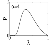
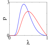
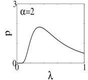
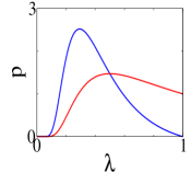
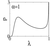
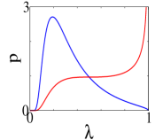
Figure 1: Probability distribution $p(\lambda)$ given in Eq. (13) for different values of $\alpha$. Distributions on the right-hand side column are for $p_{+}$ and $p_{-}$. Blue colored distributions represent released particles $p_{-}$ and red colored distributions represent trapped particles $p_{+}$.

The probability distribution $p(\lambda)$ is defined on the interval $\lambda\in[0,1]$, where $\lambda=1$ is the strength of an actual harmonic trap in dimensionless units and $\lambda=0$ represents the absence of a harmonic trap. The fact that $p(\lambda=0)=0$ for any $\alpha$ implies that there is zero probability for particles to spread out into infinity. In other words, particles always remain confined to a finite region despite there being periods when an external potential is turned off.

The behavior at $\lambda=1$ is more interesting. The probability at $\lambda=1$ exhibits a crossover at $\alpha=2$ such that

$$p(1)=\begin{cases}0&\text{$\alpha>2$}\\ \frac{1}{2}&\text{$\alpha=2$}\\ \infty&\text{$\alpha<2$}.\end{cases}$$

At $\lambda=1$, the probability is zero if fluctuations of a trap strength are sufficiently fast, such that $\alpha>2$. Then for slower fluctuations, such as $\alpha<2$, the trap is turned on for a sufficiently long time which permits particles to attain something like a temporal equilibrium, as a result the probability distribution at $\lambda=1$ diverges.

To visualize the tendency of distributions $p_{\pm}(\lambda)$ to develop different properties as $\alpha\to 0$, in Fig. (2) we plot the mean $\lambda$ corresponding to each distribution, $\langle\lambda\rangle_{\pm}$. For the limiting case $\alpha\to 0$, $\langle\lambda\rangle_{+}\to 1$ and $\langle\lambda\rangle_{-}\to 0$, and in the limit $\alpha\to\infty$, $\langle\lambda\rangle_{+}=\langle\lambda\rangle_{-}$.

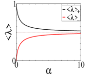
Figure 2: Average $\lambda$ for distributions $p_{+}(\lambda)$ and $p_{-}(\lambda)$.

Despite a very different shape of each $p_{\pm}(\lambda)$, the mean value of $\lambda$ for a total distribution $p(\lambda)$ is fixed at $\langle\lambda\rangle=\frac{1}{2}$ for any value of $\alpha$. This reflects the fact that on average the amount of time in which a system is in an "on" and "off" state is the same, regardless of $\alpha$. The parameter $\alpha$ only controls the rate with which the system changes between the two states but not the preference for being in a particular state.

Probability distributions for particles in different states $p_{\pm}(\lambda)$ are shown on the right-hand-side in Fig. (1). The two probabilities exhibit very different properties. These differences become greater for a slowly fluctuation harmonic trap, $\alpha\to 0$. As $\alpha$ decreases, distribution for particles in a trapped state $p_{+}$ shifts toward $\lambda=1$, resulting in a divergence, and distributions for particles in a released state shift toward $\alpha=0$, without ever reaching it. In the limit $\alpha\to\infty$, very fast fluctuation trap, the two distributions $p_{\pm}$ shift toward $\lambda=1/2$ and converge to the same functional form.

Using the superposition formula in Eq. (10) together with the formula for $p(\lambda)$ in Eq. (13), the solution of the third-order differential equation in Eq. (4) is given by

$$\rho(z)=\frac{(\alpha e/2)^{\alpha/2}}{2\Gamma(\alpha/2)}\left(\frac{1}{2\pi}\right)^{\frac{1}{2}}\int_{0}^{1}d\lambda\,\left(\frac{1}{\lambda}-1\right)^{\frac{\alpha}{2}-1}\frac{e^{-\frac{\alpha}{2\lambda}}e^{-\frac{\lambda z^{2}}{2}}}{\lambda^{3-\frac{1}{2}}}.$$ (15)

The integral in Eq. (15) cannot be evaluated except for specific discrete values of $\alpha$ corresponding to $\alpha=2n$ where $n$ is the positive integer. For $\alpha=2$, corresponding to a crossover point, the term $\left(\frac{1}{\lambda}-1\right)^{\frac{\alpha}{2}-1}$ in Eq. (15) becomes unity and $p(\lambda)$ evaluates to the following analytical form

$$\rho = \frac{1}{2}\frac{e^{-z^{2}/2}}{\sqrt{2\pi}}$$ (16)

$$+ \frac{1}{8\sqrt{2}}\left[\left(1-\sqrt{2z^{2}}\right)\text{erfc}\left[1+\frac{\sqrt{2z^{2}}}{2}\right]e^{1+\sqrt{2z^{2}}}\right]$$

$$+ \frac{1}{8\sqrt{2}}\left[\left(1+\sqrt{2z^{2}}\right)\text{erfc}\left[1-\frac{\sqrt{2z^{2}}}{2}\right]e^{1-\sqrt{2z^{2}}}\right].$$

Note that only the first term has a Gaussian form. The remaining half of contributions comes from non-Gaussian terms.

In Fig. (3) we plot $\rho(z)$ for different values of $\alpha$. For those values of $\alpha$ where no analytical expression is available, the integral in Eq. (15) is evaluated numerically. All probability distributions are in addition compared with distributions obtained from simulation based on numerical integration of the Langevin equation to confirm the correctness of analytical results.

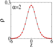
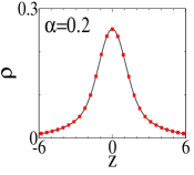
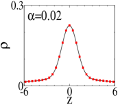
Figure 3: Distributions $\rho(z)$ calculated using Eq. (15) for different values of $\alpha$. Red data points are obtained from a simulation based on numerical integration of the Langevin equation.

The Langevin equation is integrated using the Euler method,

$$x_{+}(t+\Delta t)=x_{+}(t)-\mu Kx_{+}(t)+\xi_{+}(t)\sqrt{2D\Delta t}$$

$$x_{-}(t+\Delta t)=x_{-}(t)+\xi_{-}(t)\sqrt{2D\Delta t}$$ (17)

where $\xi_{\pm}(t)$ is the white noise with zero mean and unity variance, and $x_{+}$ and $x_{-}$ is the position of a particle in a trapped and released state, respectively. An individual particle changes from $x_{+}$ to $x_{-}$ and vice versa at the end of the time $t_{p}$ drawn from the exponential distribution $\sim e^{-t_{p}/\tau}$.

The primary non-Gaussian feature of the distributions is the spreading-out effect, giving the impression that some particles are capable of leaking from the trap. This feature becomes more pronounced for small values of $\alpha$ where particles are permitted to remain in a given state for a longer time, allowing particles to remain in a released state for longer times, which results in a greater spread.

We can get a better sense of what is happening by plotting distributions for separate states $\rho_{\pm}$. In Fig. (4) we plot the distributions $\rho_{\pm}$, calculated using the superposition formula in Eq. (10) and the distributions $p_{\pm}$ in Eq. (14).

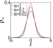
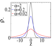
Figure 4: Distributions of trapped and released particles, $\rho_{+}$ and $\rho_{-}$, obtained from the superposition formula in Eq. (10) and the distributions $p_{\pm}$ in Eq. (14) for different parameters $\alpha$.

Distributions for particles in a trapped state $\rho_{+}$ show weaker dependence on $\alpha$. Distributions $\rho_{+}$ and $\rho_{-}$ also respond differently to decreasing $\alpha$. While $\rho_{+}$ converges to a Gaussian distribution for the trap strength $\lambda=1$, $\rho_{-}$ becomes more spread out and deviates increasingly from a Gaussian form. The spreading out of $\rho$ seen in Fig. (3) comes from particles in a released state $\rho_{-}$.

III.1 characteristic function

Even though the integral in Eq. (15) cannot be evaluated for an arbitrary $\alpha$, the characteristic function $\hat{\rho}(q)=\int_{-\infty}^{\infty}dz\,e^{-iqz}\rho(z)$ has a relatively simple algebraic form given by

$$\hat{\rho}(q)=e^{-{q^{2}}/{2}}\left[\frac{2\alpha+q^{2}}{2\alpha}\left(\frac{\alpha}{\alpha+q^{2}}\right)^{\frac{\alpha}{2}+1}\right].$$ (18)

Since the factor $e^{-{q^{2}}/{2}}$ is the characteristic function of the Boltzmann distribution, we can represent $\hat{\rho}(q)$ as

$$\hat{\rho}(q)=\hat{\rho}_{eq}(q)\hat{\rho}_{neq}(q),$$

where $\hat{\rho}_{eq}(q)=e^{-{q^{2}}/{2}}$, and $\hat{\rho}_{neq}(q)$ captures non-equilibrium contributions. As the product of two Fourier transformed function corresponds to the convolution in the real space, we could represent $\rho$ as

$$\rho(z)=\int dz^{\prime}\,\rho_{eq}(z-z^{\prime})\rho_{neq}(z^{\prime}),$$ (19)

and because the convolution construction implies the presence of two independent random processes, we could interpret $\rho_{neq}$ as some type of random process. At the crossover $\alpha=2$, $\rho_{neq}$ is found to have a simple form given by

$$\rho_{neq}=\frac{e^{-|z|\sqrt{2}}}{8}\left(3\sqrt{2}+2z\right),$$ (20)

and the convolution formula in Eq. (19) smears out this result into the formula in Eq. (16). Despite Gaussian smearing, the asymptotic behavior of $\rho$ should be dominated by the exponential form of $\rho_{neq}$, which indicates that $\rho$ has different asymptotic behavior than that of a Boltzmann distribution.

IV Time-dependent harmonic trap

In this section we provide justification for the superposition formula in Eq. (10). To provide such a justification, we consider a harmonic potential with a general time-dependent strength,

$$u(x,t)=\frac{K(t)x^{2}}{2}.$$ (21)

It might seem that the time-dependent distribution of such a system is tricky to calculate, but we claim that it is a Gaussian function at all times,

$$\rho(x,t)=\sqrt{\frac{\mu K_{eff}}{2\pi D}}\exp\left[-\frac{\mu K_{eff}}{D}\frac{x^{2}}{2}\right].$$ (22)

If this claim is correct, then all we need to calculate to derive the expression for $\rho(x,t)$ is the time-dependent effective strength $K_{eff}(t)$ such that $K_{eff}(t)\neq K(t)$ (unless $K(t)$ varies very slowly). The only constraint we introduce is that at $t=0$, $\rho(x,t)$ is a Gaussian function corresponding to some initial effective strength $K_{0}=K_{eff}(0)$.

To calculate $K_{eff}$, we insert the Gaussian distribution in Eq. (22) into the corresponding time-dependent Fokker-Planck equation,

$$\dot{\rho}=\mu K(t)[x\rho]^{\prime}+D\nabla^{2}\rho,$$ (23)

which yields the following equation

$$\mu K-\mu K_{eff}=\frac{1}{2}\frac{d\ln K_{eff}}{dt},$$ (24)

for which the solution is

$$K_{eff}(t)=\frac{K_{0}}{e^{-2\int_{0}^{t}dt^{\prime}\,\mu K(t^{\prime})}+2\mu K_{0}\int_{0}^{t}dt^{\prime}\,e^{-2\int_{t^{\prime}}^{t}dt^{\prime\prime}\,\mu K(t^{\prime\prime})}}.$$ (25)

The fact that Eq. (24) can be solved implies that the Gaussian distribution in Eq. (22) is a correct time-dependent distribution and a solution of Eq. (23).

If $K(t)$ changes in some periodic, quasi-periodic, or any other repetitive fashion, then it should be possible to obtain an average time-independent distribution defined as

$$\rho(x)=\lim_{t\to\infty}\frac{1}{t}\int_{0}^{t}ds\,\rho(x,s).$$ (26)

And since it was determined that the distribution at all times has a Gaussian form, we could represent $\rho(x)$ defined above as a superposition of Gaussian distributions,

$$\rho(x)=\lim_{t\to\infty}\frac{1}{t}\int_{0}^{t}ds\,\rho_{G}(z,s)=\int_{0}^{1}d\lambda\,p(\lambda)\rho_{G}(z;\lambda),$$ (27)

where the probability distribution $p(\lambda)$ depends on a specific evolution of $K_{eff}(t)$. The superposition formula in Eq. (10) is simply a reflection of this underlying behavior.

In the case that $K(t)$ changes discontinuously as $K_{0}\to K_{1}$, Eq. (25) reduces to

$$K_{eff}(t)=\frac{K_{0}K_{1}}{K_{0}-(K_{0}-K_{1})e^{-2\mu K_{1}t}}.$$ (28)

In the model considered in this work, the strength of the harmonic potential changes between two discrete values, $0$ and $K$, corresponding to the strength of the actual trap.

Using Eq. (28), we could calculate the evolution of $K_{eff}(t)$ as $K(t)$ fluctuates between zero and the actual strength of a trap, and where the trap persists in a given state for the length of time drawn from the exponential distribution. The resulting evolution of $K_{eff}$ is shown in Fig. (5) for different values of $\alpha$.

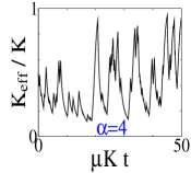
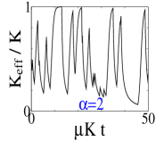
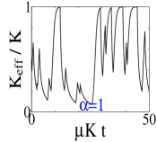
Figure 5: $K_{eff}$ of a fluctuating trap for different $\alpha=1/\mu K\tau$. The initial value is $K_{eff}(0)=K/2$ for all figures.

For $\alpha=4$, which is above the point of crossover, $K_{eff}$ fails to get close to $K$ due to rapid fluctuations of a trap. This explains why the probability distribution $p(\lambda)$ in Fig. (1) for the same value of $\alpha$ is zero at $K_{eff}/K=\lambda=1$. For $\alpha=1$, which is below the crossover, $K_{eff}$ can stay very close to $K$ for extended periods. This gives rise to a divergence in $p(\lambda)$ at $\lambda=1$ seen in Fig. (1) for the same value of $\alpha$.

It is possible to obtain the distribution $p(\lambda)$ from the evolution of $K_{eff}(t)$ using $p(\lambda)\sim\lim_{t\to\infty}\frac{1}{t}\frac{dt}{d\lambda}$, where $\lambda(t)=K_{eff}(t)/K$.

V Extension to higher dimensions

It is straightforward to extend the results in Sec. (IV) to an arbitrary dimension $d$. Given a time-dependent harmonic potential,

$$u(x,t)=\frac{K(t)r^{2}}{2},$$ (29)

where $r^{2}=\sum_{i=1}^{d}x_{i}^{2}$ is the radial distance from a trap center for a system in dimension $d$. We next assume that the time-dependent distribution has a Gaussian form at all times,

$$\rho(r,t)=\left(\frac{\mu K_{eff}}{2\pi D}\right)^{d/2}\exp\left[-\frac{\mu K_{eff}}{D}\frac{r^{2}}{2}\right],$$ (30)

and to obtain an expression for $K_{eff}(t)$, we insert the Gaussian distribution above into the corresponding Fokker-Planck equation,

$$\dot{\rho}=\mu K(t)\mbox{\boldmath$\nabla$}\cdot({\bf r}\rho)+D\nabla^{2}\rho.$$ (31)

Such a procedure recovers the relation in Eq. (24) for which the solution is the expression in Eq. (25). This proves that $K_{eff}(t)$ in Eq. (25) is valid for any dimension.

Other results in this work can also be extended to an arbitrary dimension. The Fokker-Planck equation for the fluctuating potential model, analogous to Eq. (2) but for an arbitrary dimension, is given by

$$\dot{\rho}_{+}=\mu K\mbox{\boldmath$\nabla$}\cdot[{\bf r}\rho_{+}]+D\nabla^{2}\rho_{+}+\frac{1}{\tau}\left(\rho_{-}-\rho_{+}\right)$$

$$\dot{\rho}_{-}=D\nabla^{2}\rho_{-}-\frac{1}{\tau}\left(\rho_{-}-\rho_{+}\right).$$ (32)

For a stationary state and in reduced units the two equations above become

$$0=\mbox{\boldmath$\nabla$}\cdot[{\bf s}\rho_{+}]+\nabla^{2}\rho_{+}+\alpha\left(\rho_{-}-\rho_{+}\right)$$

$$0=\nabla^{2}\rho_{-}-\alpha\left(\rho_{-}-\rho_{+}\right),$$ (33)

where ${\bf s}={\bf r}\sqrt{\frac{\mu K}{D}}$.

The moments of stationary distributions can be obtained by operating on both equations in Eq. (33) with $\int d{\bf r}\,r^{d-1}\,r^{2n}$. The resulting expressions for the second moment are

$$\langle s^{2}\rangle_{+}=2d$$

$$\langle s^{2}\rangle_{-}=2d\left(1+\frac{1}{\alpha}\right)$$

$$\langle s^{2}\rangle=d\left(2+\frac{1}{\alpha}\right).$$ (34)

By combining the two equations in Eq. (33) we obtain a third-order differential equation,

$$0=-\alpha s^{3}\rho+[3-d-(2\alpha+1-d)s^{2}]\rho^{\prime}-[3-d-s^{2}]s\rho^{\prime\prime}+s^{2}\rho^{\prime\prime\prime}.$$ (35)

Note that by setting $d=1$ we recover Eq. (4). To find the solution of the above equation, we represent a stationary distribution as a superposition of Gaussian distributions,

$$\rho(s)=\int_{0}^{1}d\lambda\,p(\lambda)\rho_{G}(s;\lambda),$$ (36)

where

$$\rho_{G}(s;\lambda)=\left(\frac{\lambda}{2\pi}\right)^{d/2}e^{-\lambda s^{2}/2}.$$ (37)

Since it was determined that $K_{eff}(t)$ is independent of $d$, and since it is possible to obtain the probability distribution $p(\lambda)$ from the evolution of $K_{eff}(t)$, we conclude that the expression for $p(\lambda)$ in Eq. (13) is valid for all $d$. This means that any dependence on $d$ comes from the Gaussian distribution in Eq. (37), and the solution of the third-order differential equation in Eq. (35) is given by

$$\rho(s)=\frac{(\alpha e/2)^{\alpha/2}}{2\Gamma(\alpha/2)}\left(\frac{1}{2\pi}\right)^{\frac{d}{2}}\int_{0}^{1}d\lambda\,\left(\frac{1}{\lambda}-1\right)^{\frac{\alpha}{2}-1}\frac{e^{-\frac{\alpha}{2\lambda}}e^{-\frac{\lambda s^{2}}{2}}}{\lambda^{3-\frac{d}{2}}}.$$ (38)

The solution is not limited to integer values of $d$ and applies to any value of $d$.

VI Quantities of physical interest

VI.1 potential energy

In this section we look into physical quantities of the model, starting with the average potential energy $\langle u\rangle_{\pm}=K\langle r^{2}\rangle_{\pm}/2$. Using the moments in Eq. (34), the potential energy for particles in each state is found to be

$$\langle u\rangle_{+}=dk_{B}T,$$

$$\langle u\rangle_{-}=0.$$ (39)

The potential energy of particles in a released state is zero since the trap is switched off. Another interesting observation is that the potential energy of particles in a trapped state does not depend on the rate parameter $\alpha$. Adding the two contributions, the total potential energy is found to be the same as that for a system in equilibrium,

$$\langle u\rangle=\frac{dk_{B}T}{2}.$$ (40)

The imperfect harmonic potential might considerably alter stationary distributions but the average potential energy is unaffected.

VI.2 flux

We next consider flux, which for particles in a each state and for $d=1$ is given by

$$j_{-}=-D\rho^{\prime}_{-},~{}~{}~{}~{}~{}j_{+}=-\mu Kx\rho_{+}-D\rho^{\prime}_{+},$$ (41)

and is such that the total flux is zero everywhere, $j=j_{+}+j_{-}=0$.

In Fig. (6) we plot flux for particles in a released state, $j_{-}$, in dimensionless units given by $j_{-}(z)=-\rho^{\prime}_{-}(z)$. (No insight is gained by plotting $j_{+}$ since $j_{+}=-j_{-}$). The first observation is that released particles move away from the trap center, which is expected. The second observation is that the magnitude of the flux increases with increased rate $\alpha$. This makes sense as released particles tend to be more compressed when $\alpha$ is large and so diffusion away from the trap center when particles are released should be greater.

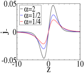
Figure 6: Flux for particles released from the trap. Flux for particles in a trapped state, not shown in the figure, is $j_{+}=-j_{-}$.

As both fluxes have the same functional form, a better insight could be gained by looking into the local velocity, in dimensionless units given by

$$v_{+}=\frac{j_{+}}{\rho_{+}}=-[\ln\rho_{+}]^{\prime}-z,~{}~{}~{}~{}~{}~{}v_{-}=\frac{j_{-}}{\rho_{-}}=-[\ln\rho_{-}]^{\prime}.$$ (42)

Note that the velocity in a trapped state has an additional linear term resulting from an external force. The other term in each expression comes from diffusion.

Local velocities are shown in Fig. (7). For particles in a trapped state we plot $v_{+}+z$ to subtract contributions of an external force. Consequently, the two plots amount to $-[\ln\rho_{\pm}]^{\prime}$ and represent diffusional component of a local velocity.

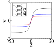
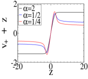
Figure 7: Local velocity for different values of $\alpha$. For trapped particles we plot $v_{+}+z$ to subtract contributions of an external force, as a result, both quantities represent diffusional component of a local velocity. In both cases this corresponds to plotting $-[\ln\rho_{\pm}]^{\prime}$.

The most striking feature is that the local velocity does not vanish at infinity but saturate to a non-zero constant. Since the quantity that is plotted is $-[\ln\rho_{\pm}]^{\prime}$, this implies that distributions $\rho_{\pm}$ decay exponentially. Such an asymptotic behavior has been hinted at in Sec. (III.1) and was proven for $\alpha=2$ in Eq. (20).

VI.3 entropy production rate

One feature of an active system is that it generates heat that is dissipated into reservoir. By measuring the rate of heat that is dissipated, we could quantify a distance of how far from equilibrium a system is. The rate of heat dissipation, $\langle\dot{q}\rangle$, is, in addition, related to the entropy production rate $\Pi$ via the relation $T\Pi\equiv\langle\dot{q}\rangle$ Frydel23a .

A formula for the dissipation of heat can be obtained from the drag force a particle experiences when it moves through a dissipating medium, ${\bf F}_{d}=-\mu^{-1}{\bf v}$, where ${\bf v}$ is the velocity vector. An instantaneous rate of heat dissipation is then given by $\dot{q}=\mu^{-1}v^{2}$. However, when calculating the average rate of heat dissipation, we need to subtract equilibrium contributions, $\langle\dot{q}\rangle=\mu^{-1}\langle v^{2}\rangle-\mu^{-1}\langle v^{2}\rangle_{eq}$, since these contributions are not truly dissipated but are recovered at some point in the form of thermal fluctuations as a result of the fluctuation-dissipation relation. Since $\langle v^{2}\rangle_{eq}=dk_{B}T/m$, we can write

$$\langle\dot{q}\rangle=\frac{1}{\mu}\left[\langle v^{2}\rangle-\frac{dD}{\tau_{r}}\right],$$ (43)

where $\tau_{r}=m\mu$ is the inertial relaxation and $m$ is the mass of a particle. For overdamped dynamics there is no inertia and $\tau_{r}=0$.

To calculate $\langle v^{2}\rangle$ we need to formulate our model in the underdamped regime. The overdamped regime can then be recovered by setting $\tau_{r}=0$. We find the following result for the overdamped regime:

$$\langle v^{2}\rangle-\frac{dD}{\tau_{r}}=\frac{d\mu KD}{2}.$$ (44)

The derivation of the above formula requires that we formulate the problem using the Kramer’s equation, instead of the Fokker-Planck equation Frydel23a . The details of the derivation can be found in Appendix D.

Since $\langle v^{2}\rangle$ is proportional to the kinetic energy, the term on the right-hand-side in Eq. (44) can be seen as the excess kinetic energy that results due to trap fluctuations. The formula, however, does not depend on the rate of the trap fluctuations $\alpha$. This means that the kinetic energy also does not depend on $\alpha$, similar to the potential formula energy in Eq. (40).

Inserting Eq. (44) in Eq. (43) yields

$$T\Pi\equiv\langle\dot{q}\rangle=\frac{dDK}{2}.$$ (45)

The result in Eq. (45) shows that the dissipation of heat is a function of the temperature and the trap strength and is completely independent of the rate parameter $\alpha$ that controls fluctuations of the harmonic trap. This independence implies that even in the limit $\alpha\to\infty$, where a stationary distribution converges to the Gaussian distribution for the trap strength $K/2$, the heat continues to be dissipated in the same way as for any other value of $\alpha$ and the system is always at the same distance from equilibrium.

VII Conclusion

This work considers an ideal gas confined to a harmonic trap $u=Kr^{2}/2$ with time dependent strength $K\equiv K(t)$. It is demonstrated that the time dependent distribution of such a system $\rho(x,t)$ has a Gaussian form at all times, corresponding to some effective strength of the harmonic potential, $K_{eff}(t)\neq K(t)$.

We are interested in a specific time evolution of $K(t)$ such that it changes discontinuously between two discrete values, $0$ and $K$, and where the time during which a trap remains in a given state is drawn from an exponential distribution $\sim e^{-t_{p}/\tau}$.

A stationary distribution of this system can be obtained from a third-order differential equation, the solution of which is represented as a superposition of Gaussian distributions for different strengths of a harmonic trap, $\rho(x)=\int_{0}^{K}dK^{\prime}\,p(K^{\prime})\rho_{G}(x;K^{\prime})$. The reason for the superposition can be traced back to the fact that a time-dependent distribution at all times has a Gaussian form.

The probability distribution $p(K)$ can be obtained and analyzed. The resulting algebraic expression for $p(K)$ exhibits a crossover at $\tau=2/\mu K$. For $\tau>2\mu K$, the distribution $p(K^{\prime})$ diverges at $K^{\prime}=K$, indicating that a fraction of particles comes close to an equilibrium-like behavior. The divergence disappears for $\tau<2/\mu K$, and for very small $\tau$, a stationary distribution converges to a Gaussian form for a trap with the strength which is half the strength of the physical trap, $K/2$.

The primary feature of the resulting stationary distribution $\rho(x)=\int_{0}^{K}dK^{\prime}\,p(K^{\prime})\rho_{G}(x;K^{\prime})$ is the spreading-out effect, which is understood to be the result of a trap being turned off. Since the period during which a trap is turned off increases with $\tau$, the distributions tend to be more spread out for larger $\tau$. As a result of spreading-out, the asymptotic behavior of $\rho(x)$ is dominated by an exponential decay.

The spreading-out feature of the current model is different from typical active particles that tend, rather than to spread-out and penetrate the trap boundaries, to accumulate at the trap boundaries. This behavior is seen for RTP and ABP particles. The accumulation of particles at the boundaries leads to bimodal stationary distributions, with excess of particles close to boundaries and depletion of particles near a trap center. These models exhibit crossover when a stationary distribution changes from a bimodal to unimodal distribution.

VIII DATA AVAILABILITY

The data that support the findings of this study are available from the corresponding author upon reasonable request.

Appendix A Derivation of Eq. (4)

In the section we provide details how the two coupled equations in Eq. (3), which we reproduce below,

$$0=[z\rho_{+}]^{\prime}+\rho_{+}^{\prime\prime}+\alpha\left(\rho_{-}-\rho_{+}\right),$$

$$0=\rho_{-}^{\prime\prime}+\alpha\left(\rho_{+}-\rho_{-}\right),$$ (46)

are combined to yield the third-order differential equation in Eq. (4). Adding and subtracting the two equations yield

$$0=\frac{1}{2}[z\rho]^{\prime}+\frac{1}{2}[z\sigma]^{\prime}+\rho^{\prime\prime},$$

$$0=\frac{1}{2}[z\rho]^{\prime}+\frac{1}{2}[z\sigma]^{\prime}+\sigma^{\prime\prime}-2\alpha\sigma,$$ (47)

where $\rho=(\rho_{+}+\rho_{-})/2$ and $\sigma=(\rho_{+}-\rho_{-})/2$. From the first equation we get $z\sigma=-z\rho-2\rho^{\prime}+\text{const},$ where $\text{const}=0$ as a result of the even symmetry of $\rho(z)$. From this we can generate a sequence of expressions

$$\sigma=-\rho-\frac{2}{z}\rho^{\prime},$$

$$\sigma^{\prime}=-\rho^{\prime}+\frac{2}{z^{2}}\rho^{\prime}-\frac{2}{z}\rho^{\prime\prime},$$

$$\sigma^{\prime\prime}=-\rho^{\prime\prime}-\frac{4}{z^{3}}\rho^{\prime}+\frac{4}{z^{2}}\rho^{\prime\prime}-\frac{2}{z}\rho^{\prime\prime\prime}.$$ (48)

Inserting these expressions into the second equation in Eq. (47) recovers Eq. (4).

Appendix B Recurrence relation

This section shows how even moments, given by

$$\langle z^{2n}\rangle_{\pm}=\int_{-\infty}^{\infty}dz\,z^{2n}\rho_{\pm}(z)$$

can be obtained from the two equations in Eq. (3), which we repeat below for clarity:

$$0=[z\rho_{+}]^{\prime}+\rho_{+}^{\prime\prime}+\alpha\left(\rho_{-}-\rho_{+}\right)$$

$$0=\rho_{-}^{\prime\prime}+\alpha\left(\rho_{+}-\rho_{-}\right).$$ (49)

To convert the two equations into the recurrence relation, we operate on both equation with $\int_{-\infty}^{\infty}dz\,z^{2n+2}$. This results in the following two coupled recurrence relations:

$$0=-(2n+2)m_{n+1}^{+}+(2n+2)(2n+1)m_{n}^{+}+\alpha\left(m_{n+1}^{-}-m_{n+1}^{+}\right)$$

$$0=(2n+2)(2n+1)m_{n}^{-}+\alpha\left(m_{n+1}^{+}-m_{n+1}^{-}\right),$$ (50)

where $m_{n}^{+}=\langle z^{2n}\rangle_{+}$ and $m_{n}^{-}=\langle z^{2n}\rangle_{-}$. After rearrangement, the two equations become

$$m_{n+1}^{+}=(2n+1)(m_{n}^{+}+m_{n}^{-})$$

$$m_{n+1}^{+}=(2n+1)\left(m_{n}^{+}-m_{n}^{-}\right)-\frac{2\alpha}{(2n+2)}\left(m_{n+1}^{+}-m_{n+1}^{-}\right).$$

The initial terms of both sequences are $m_{0}^{+}=m_{0}^{-}=1$ and the remaining terms are obtained from the recurrence relations above.

Appendix C Derivation of Eq. (11)

In this section we demonstrate how combining the two equations in Eq. (11), which we reproduce below,

$$0=[\lambda(\lambda-1)p_{+}]^{\prime}+\frac{\alpha}{2}(p_{-}-p_{+})$$

$$0=[\lambda^{2}p_{-}]^{\prime}+\frac{\alpha}{2}(p_{+}-p_{-}),$$ (51)

leads to the first order differential equation in Eq. (14). Adding and subtracting the two equations yield

$$0=[\lambda(2\lambda-1)p]^{\prime}-\lambda\sigma^{\prime}$$

$$0=2[\lambda^{2}\sigma]^{\prime}-\lambda p^{\prime}-\lambda\sigma^{\prime}-2\alpha\sigma,$$ (52)

where $p=(p_{+}+p_{-})/2$ and $\sigma=(p_{+}-p_{-})/2$. From the first equation we get $\sigma=(2\lambda-1)p$ and from which we generate the consecutive expressions

$$\sigma=(2\lambda-1)p,$$

$$\sigma^{\prime}=2p+(2\lambda-1)p^{\prime},$$ (53)

Inserting these expressions into the second equation in Eq. (52) recovers Eq. (14).

Appendix D Derivation of $\langle v^{2}\rangle$

To obtain the expression for $\langle v^{2}\rangle$, we need to formulate our model within underdamped dynamics. This means that we need to formulate the system within Kramer’s equation, which is the type of Fokker-Planck equation for the underdamped regime Frydel23a . The evolution of the distributions $\rho_{\pm}\equiv\rho_{\pm}({\bf r},{\bf v},t)$ is governed by the following Kramer’s equations:

$$\frac{\partial\rho_{+}}{\partial t} = -{\bf v}\cdot\mbox{\boldmath$\nabla$}_{r}\rho_{+}+\frac{1}{\tau_{r}}\mbox{\boldmath$\nabla$}_{v}\cdot\left[\left(\mu K{\bf r}+{\bf v}\right)\rho_{+}\right]+\frac{D}{\tau_{r}^{2}}\nabla_{v}^{2}\rho_{+}$$

$$+ \frac{1}{\tau}(\rho_{-}-\rho_{+})$$

$$\frac{\partial\rho_{-}}{\partial t} = -{\bf v}\cdot\mbox{\boldmath$\nabla$}_{r}\rho_{-}+\frac{1}{\tau_{r}}\mbox{\boldmath$\nabla$}_{v}\cdot\left[{\bf v}\rho_{-}\right]+\frac{D}{\tau_{r}^{2}}\nabla_{v}^{2}\rho_{-}+\frac{1}{\tau}(\rho_{+}-\rho_{-}),$$

and we recall that $\tau_{r}=m\mu$ is the inertial relaxation, $m$ is a particle mass, and the overdamped regime is recovered for $\tau_{r}=0$.

To calculate $\langle v^{2}\rangle$, or other average quantities of interest, we operate on the stationary Kramer’s equation, $\dot{\rho}=0$, with an integral operator $\hat{O}_{g}=\int d{\bf v}\int d{\bf r}\,\,g({\bf r},{\bf v}),$ where the function $g$ is going to be defined later. Using integration by parts, the terms of a transformed Kramer’s equation can be represented as average quantities, designated by the angular brackets $\langle\dots\rangle=\int d{\bf v}\int d{\bf r}\,\,(\dots)$. The resulting two equations are

$$0 = \langle{\bf v}\cdot\mbox{\boldmath$\nabla$}_{r}g\rangle_{+}-\frac{1}{\tau_{r}}\langle\left(\mu K{\bf r}+{\bf v}\right)\cdot\mbox{\boldmath$\nabla$}_{v}g\rangle_{+}+\frac{D}{\tau_{r}^{2}}\langle\nabla_{v}^{2}g\rangle_{+}$$

$$+ \frac{\langle g\rangle_{-}}{\tau}-\frac{\langle g\rangle_{+}}{\tau}$$

$$0=\langle{\bf v}\cdot\mbox{\boldmath$\nabla$}_{r}g\rangle_{-}-\frac{1}{\tau_{r}}\langle{\bf v}\cdot\mbox{\boldmath$\nabla$}_{v}g\rangle_{-}+\frac{D}{\tau_{r}^{2}}\langle\nabla_{v}^{2}g\rangle_{-}+\frac{\langle g\rangle_{+}}{\tau}-\frac{\langle g\rangle_{-}}{\tau}.$$

Using $g=v^{2}$, $g=r^{2}$, and $g={\bf r}\cdot{\bf v}$, we can generate from the relation above six equations involving six unknown average quantities,

$$0=-\frac{2}{\tau_{r}}\langle v^{2}\rangle_{+}+\frac{2dD}{\tau_{r}^{2}}-\frac{1}{\tau}\langle v^{2}\rangle_{+}+\frac{1}{\tau}\langle v^{2}\rangle_{-}-\frac{2\mu K}{\tau_{r}}\langle{\bf r}\cdot{\bf v}\rangle_{+}$$

$$0=-\frac{2}{\tau_{r}}\langle v^{2}\rangle_{-}+\frac{2dD}{\tau_{r}^{2}}-\frac{1}{\tau}\langle v^{2}\rangle_{-}+\frac{1}{\tau}\langle v^{2}\rangle_{+}$$

$$0=\langle v^{2}\rangle_{+}+\frac{1}{\tau_{r}}\langle{\bf v}\cdot{\bf r}\rangle_{+}-\frac{1}{\tau}\langle{\bf v}\cdot{\bf r}\rangle_{+}+\frac{1}{\tau}\langle{\bf v}\cdot{\bf r}\rangle_{-}-\frac{\mu K}{\tau_{r}}\langle r^{2}\rangle_{+}$$

$$0=\langle v^{2}\rangle_{-}-\frac{1}{\tau_{r}}\langle{\bf v}\cdot{}\bf r\rangle_{-}-\frac{1}{\tau}\langle{\bf v}\cdot{\bf r}\rangle_{-}+\frac{1}{\tau}\langle{\bf v}\cdot{\bf r}\rangle_{+}$$

$$0=2\langle{\bf v}\cdot{\bf r}\rangle_{+}-\frac{1}{\tau}\langle r^{2}\rangle_{+}+\frac{1}{\tau}\langle r^{2}\rangle_{-}$$

$$0=2\langle{\bf v}\cdot{\bf r}\rangle_{-}-\frac{1}{\tau}\langle r^{2}\rangle_{-}+\frac{1}{\tau}\langle r^{2}\rangle_{+}.$$ (54)

After solving the system of coupled equations above, we get

$$\langle v^{2}\rangle-\frac{dD}{\tau_{r}}=-\frac{d\tau D\mu K(\tau_{r}+\tau)}{\mu K\tau_{r}^{2}\tau-4\tau_{r}^{2}-6\tau_{r}\tau-2\tau^{2}},$$ (55)

which for the overdamped regime $\tau_{r}=0$ reduces to

$$\langle v^{2}\rangle-\frac{dD}{\tau_{r}}=\frac{dD\mu K}{2}.$$ (56)

Since $\langle v^{2}\rangle_{eq}=\frac{dD}{\tau_{r}}$, and since $\langle v^{2}\rangle$ is proportional to the kinetic energy, we can think of the above quantity as representing the excess kinetic energy that arises due to fluctuations of a harmonic trap.

References

- (1) J. Tailleur and M. E. Cates, Statistical Mechanics of Interacting Run-and-Tumble Bacteria, Phys. Rev. Lett. 100, 218103 (2008).
- (2) J. Tailleur and M. E. Cates, Sedimentation, trapping, and rectification of dilute bacteria, Europhys. Lett. 86, 60002 (2009).
- (3) M. R. Evans and S. N. Majumdar, Run and tumble particle under resetting: a renewal approach, J. Phys. A: Math. Theor. 51 475003 (2018).
- (4) K. Malakar, V. Jemseena, A. Kundu, K. V. Kumar, S. Sabhapandit, S. N. Majumdar, S. Redner, and A. Dhar, Steady state, relaxation and first-passage properties of a run-and-tumble particle in one-dimension, J. Stat. Mech.: Theory Exp. 043215 (2018).
- (5) A. Dhar, A. Kundu, S. N. Majumdar, S. Sabhapandit, and G. Schehr, Run-and-tumble particle in one-dimensional confining potentials: Steady-state, relaxation, and first-passage properties, Phys. Rev. E 99, 032132 (2019).
- (6) U. Basu, S. N. Majumdar, A. Rosso, S. Sabhapandit, and G. Schehr, Exact stationary state of a run-and-tumble particle with three internal states in a harmonic trap, J. Phys. A 53, 09LT01 (2020).
- (7) A. Villa-Torrealba, C.l Chávez-Raby, P. de Castro, and R. Soto, Run-and-tumble bacteria slowly approaching the diffusive regime, Phys. Rev. E 101, 062607 (2020),
- (8) N. Razin, Entropy production of an active particle in a box, Phys. Rev. E (R) 102, 030103(R) (2020).
- (9) D. Frydel, Generalized run-and-tumble model for an arbitrary distribution of velocities in 1D geometry, J. Stat. Mech. 103, 052603 (2021).
- (10) D. Frydel, Kuramoto model with run-and-tumble dynamics, Phys. Rev. E 104, 024203 (2021).
- (11) N. R. Smith and O. Farago, Nonequilibrium steady state for harmonically confined active particles, Phys. Rev. E 106, 054118 (2022).
- (12) D. Frydel, The four-state RTP model: exact solution at zero temperature, Phys. Fluids 34, 027111 (2022).
- (13) C. Roberts and Z. Zhen, Run-and-tumble motion in a linear ratchet potential: Analytic solution, power extraction, and first-passage properties, Phys. Rev. E 108, 014139 (2023).
- (14) O. Farago and N. R. Smith, Confined run-and-tumble particles with non-Markovian tumbling statistics, Phys. Rev. E 109, 044121 (2024),
- (15) T. Pietrangeli, C. Ybert, C. Cottin-Bizonne, and F. Detcheverry, Optimal run-and-tumble in slit-like confinement, Phys. Rev. Research 6, 023028 (2024).
- (16) B. Loewe, T. Kozhukhov and, T. N. Shendruk Anisotropic run-and-tumble-turn dynamics, Soft Matter 20, 1133 (2024).
- (17) K. Malakar, A. Das, A. Kundu, K. V. Kumar, and A. Dhar Steady state of an active Brownian particle in a two-dimensional harmonic trap, Phys. Rev. E 101, 022610 (2020).
- (18) M. Caraglio, T. Franosch, Analytic solution of an active brownian particle in a harmonic well, Phys. Rev. Lett. 129, 158001, (2022).
- (19) G. Szamel, Self-propelled particle in an external potential: Existence of an effective temperature, Phys, Rev. E 90, 012111 (2014).
- (20) S. Shankar and M. C. Marchetti, Hidden entropy production and work fluctuations in an ideal active gas, Phys. Rev. E 98, 020604(R) (2018).
- (21) F. J. Sevilla, R. F. Rodríguez, and J. R. Gomez-Solano, Generalized Ornstein-Uhlenbeck model for active motion, Phys. Rev. E 100, 032123 (2019).
- (22) D. Martin, J. O’Byrne, M. E. Cates, É. Fodor, C. Nardini, J. Tailleur, and F. van Wijland Statistical mechanics of active Ornstein-Uhlenbeck particles, Phys. Rev. E 103, 032607 (2021).
- (23) L. Caprini, U. M. B. Marconi, and A. Vulpiani, Linear response and correlation of a self-propelled particle in the presence of external fields, J. Stat. Mech.: Theory Exp. 033203 (2018).
- (24) G H Philipp Nguyen, Active Ornstein–Uhlenbeck model for self-propelled particles with inertia, J. Phys.: Condens. Matter 34, 035101 (2022).
- (25) Y. Sokolov, D. Frydel, D. G. Grier, H. Diamant, Y. Roichman, Hydrodynamic pair attractions between driven colloidal particles, Phys. Rev. Lett. 107, 158302 (2011).
- (26) S. C. Takatori, R. De Dier, J. Vermant, and J. F. Brady, Acoustic trapping of active matter, Nat. Commun. 7, 10694 (2016).
- (27) R. Goerlich, M. Li, S. Albert, G. Manfredi, P. Hervieux, and C. Genet, Noise and ergodic properties of Brownian motion in an optical tweezer: Looking at regime crossovers in an Ornstein-Uhlenbeck process, Phys. Rev. E 103, 032132 (2021).
- (28) I. Buttinoni, L. Caprini, L. Alvarez , F. J. Schwarzendahl, and H. Löwen, Active colloids in harmonic optical potentials, EPL 140, 27001 (2022).
- (29) R. Goerlich, L.B. Pires, G. Manfredi, P.A. Hervieux, C. Genet, Harvesting information to control nonequilibrium states of active matter, Phys. Rev. E 106, 054617, (2022).
- (30) O. Chor, A. Sohachi, R. Goerlich, E. Rosen, S. Rahav, and Y. Roichman Many-body Szilárd engine with giant number fluctuations, Phys. Rev. Research 5, 043193 (2023).
- (31) D. Frydel, Positing the problem of stationary distributions of active particles as third-order differential equation, Phys. Rev. E 106, 024121 (2022).
- (32) D. Frydel, Run-and-tumble oscillator: Moment analysis of stationary distributions, Phys. Fluids 35, 101905 (2023).
- (33) D. Frydel, Active oscillator: Recurrence relation approach , Phys. Fluids 36, 011910 (2024).
- (34) H.Kleinert, Path Integrals in Quantum Mechanics, Statistics, Polymer Physics and Financial Markets (World Scientific, Singapore, 2004).
- (35) Petr Jizba and Hagen Kleinert, Superpositions of probability distributions, Phys. Rev. E 78, 031122 (2008).
- (36) C. Beck, Dynamical Foundations of Nonextensive Statistical Mechanics, Phys. Rev. Lett. 87, 180601 (2001).
- (37) J. M. Parrondo, J. M. Horowitz, and T. Sagawa, Thermodynamics of information, Nat. Phys. 11, 131 (2015).
- (38) T. Sagawa and M. Ueda, Second law of thermodynamics with discrete quantum feedback control, Phys. Rev. Lett. 100, 080403 (2008).
- (39) F. J. Cao and M. Feito, Thermodynamics of feedback controlled systems, Phys. Rev. E 79, 041118 (2009).
- (40) J. M. Horowitz and S. Vaikuntanathan, Nonequilibrium detailed fluctuation theorem for repeated discrete feedback, Phys. Rev. E 82, 061120 (2010).
- (41) T. Sagawa and M. Ueda, Generalized Jarzynski equality under nonequilibrium feedback control, Phys. Rev. Lett. 104, 090602 (2010).
- (42) M. Ponmurugan, Generalized detailed fluctuation theorem under nonequilibrium feedback control, Phys. Rev. E 82, 031129 (2010).
- (43) Y. Fujitani and H. Suzuki, Jarzynski equality modified in the linear feedback system, J. Phys. Soc. Jpn. 79, 104003 (2010).
- (44) A. Kundu, Nonequilibrium fluctuation theorem for systems under discrete and continuous feedback control, Phys. Rev. E 86, 021107 (2012).
- (45) Seshadev Padhi and Smita Pati, Theory of Third-Order Differential Equations, (Springer Science and Business Media, 2013).
- (46) D. Frydel, Entropy production of active particles formulated for underdamped dynamics, Phys. Rev. E 107, 014604 (2023).
- (47) D. Frydel, Intuitive view of entropy production of ideal run-and-tumble particles, Phys. Rev. E 105, 034113 (2022).