Computing $k$-means in mixed precision

Abstract

The $k$-means algorithm is one of the most popular and critical techniques in data mining and machine learning, and it has achieved significant success in numerous science and engineering domains. Computing $k$-means to a global optimum is NP-hard in Euclidean space, yet there are a variety of efficient heuristic algorithms, such as Lloyd’s algorithm, that converge to a local optimum with superpolynomial complexity in the worst case. Motivated by the emergence and prominence of mixed precision capabilities in hardware, a current trend is to develop low and mixed precision variants of algorithms in order to improve the runtime and energy consumption. In this paper we study the numerical stability of Lloyd’s $k$-means algorithm, and, in particular, we confirm the stability of the widely used distance computation formula. We propose a mixed-precision framework for $k$-means computation and investigate the effects of low-precision distance computation within the framework. Through extensive simulations on various data clustering and image segmentation tasks, we verify the applicability and robustness of the mixed precision $k$-means method. We find that, in $k$-means computation, normalized data is more tolerant to the reduction of precision in the distance computation, while for nonnormalized data more care is needed in the use of reduced precision, mainly to avoid overflow. Our study demonstrates the potential for the use of mixed precision to accelerate the $k$-means computation and offers some insights into other distance-based machine learning methods.

[label1]organization=Department of Numerical Mathematics, Charles University, city=Prague, postcode=186 75, country=Czech Republic

[label2]organization=Max Planck Institute for Dynamics of Complex Technical Systems, city=Magdeburg, postcode=39106, country=Germany

1 Introduction

The $k$-means algorithm has been one of the most studied algorithms in data mining and machine learning for decades, and it is still widely in use due to its simplicity. It aims to partition data into a selected number of groups such that the Sum of Squared Errors (SSE) is minimized. The $k$-means algorithm plays an important role in vector quantization [1, 2, 3], bioinfomatics [4, 5, 6], computer vision [7, 8, 9], anomaly detection [10, 11], database management [12, 13], documents classification [14], and nearest neighbor search [2]. As stated in [15], with superpolynomial runtime, $k$-means is often very slow in practice. Many techniques have therefore been proposed to enhance the $k$-means algorithm regarding speed and scalability, for example, parallelization, batch computations, etc.; associated variants include k-means++ [16], $k$-means$||$ [17], mini-batch $k$-means [18, 19], I-$k$-means-+ [20], sparse kernel $k$-means [21], and parallel $k$-means [22, 23, 24].

With the increasing availability of and support for lower-precision floating-point arithmetic beyond the IEEE Standard 64-bit double (fp64) and 32-bit single (fp32) precisions [25] in both hardware and software simulation, low-precision arithmetic operations as well as number formats, e.g., 16-bit half precision (fp16) [25], have been widely studied and exploited in numerous numerical algorithms. Low-precision floating point arithmetic offers greater throughput, reduced data communication, and less energy usage. Low-precision floating point formats have successfully been used in a number of existing works to improve computational speed, energy efficiency, and data storage costs, e.g., in solving systems of linear equations [26, 27], least squares problems [28, 29], and unsupervised learning [30, 31].

Table 1.1: Parameters for four floating point formats; $u$ denotes unit roundoff corresponding to the precision. $x_{\min}$ denotes the smallest positive normalized floating-point number, $x_{\max}$ denotes the largest finite floating-point number, $t$ denotes the number of binary digits in the significand (including the implicit leading bit), $e_{\min}$ denotes exponent of $x_{\min}$, and $e_{\max}$ denotes exponent of $x_{\max}$.

	$u$	$x_{\min}$	$x_{\max}$	$t$	$e_{\min}$	$e_{\max}$
quarter (q52)	$1.25\times 10^{-1}$	$6.10\times 10^{-5}$	$5.73\times 10^{4}$	3	-14	15
half (fp16)	$4.88\times 10^{-4}$	$6.10\times 10^{-5}$	$6.55\times 10^{4}$	11	-14	15
single (fp32)	$5.96\times 10^{-8}$	$1.18\times 10^{-38}$	$3.4\times 10^{38}$	24	-126	127
double (fp64)	$1.11\times 10^{-16}$	$2.23\times 10^{-308}$	$1.8\times 10^{308}$	53	-1022	1023

There is thus great potential for exploiting mixed precision (particularly, lower-than-working precision) computations within algorithms to mitigate the cost of data transfers and memory access in computer cores or clusters, which can improve speed and reduce energy consumption. However, low precision computations also bring greater rounding error, and an increased risk of overflow and underflow due to the resulting narrower range of representable numbers (see Table 1.1 for parameters for floating point formats used in this paper), which can lead to significant loss of stability and accuracy. To avoid or mitigate these potential issues, a scaling strategy is often necessary in the use of low precision arithmetic [32]. Also, it is often crucial to perform rounding error analysis for the algorithm in order to recognize which parts of the algorithm can be performed in low precision—we need to identify the algorithmic components where mixed precisions can be employed judiciously to make the optimal use of our computational resources and quantitatively determine the precisions to be used, so as to maintain the quality of the algorithmic outputs at a much lower cost. Much effort has therefore been devoted to the study of mixed precision algorithms; we refer to [33, 34] and [35], for example, for surveys on the recent development of methods in numerical linear algebra and deep neural network quantization.

In this work, we develop a mixed-precision $k$-means algorithm that has the potential to accelerate the $k$-means computation without degrading the output. Instead of developing a high performance implementation, our focus is on the analysis of the use of mixed precision; low-precision computations are simulated in software. Specifically, our contributions mainly include:

1. We study the numerical stability of Lloyd’s algorithm for $k$-means and confirm that the widely adopted distance computation scheme is stable.

2. We propose a mixed-precision framework for $k$-means computation. With some theoretical support, we investigate the effects of low-precision distance computations within the framework and develop a mixed-precision $k$-means method that works well on both normalized and nonnormalized data. The mixed-precision distance computing approach can be extended to other Euclidean distance-based algorithms.

The paper is organized as follows. In Section 2 we review some recent work on computing $k$-means with extra compute resources. In Section 3 we recall the definitions of a commonly-used normalization technique in machine learning. The classical $k$-means algorithm is then presented in Section 4, where we briefly discuss the computational properties of two Euclidean distance computation formulae. In Section 5 we discuss the numerical stability of Lloyd’s $k$-means method, including the stages of distance computation and center update. Subsequently, in Section 6 we propose a mixed-precision $k$-means computation framework and identify through experiments a suitable mixed-precision distance computation scheme. Numerical simulations of our algorithms on various datasets against the working-precision k-means++ algorithm are provided in Section 7. Conclusions and future directions of research are given in Section 8.

2 Related work

Although the strategy of computing in mixed-precision has been widely used and become prevalent in neural network training (see, e.g., [31, 36]), it appears the approach has not been exploited in $k$-means computation, and our work attempts to take the first step and provide some insight into its use via rounding error analysis. Despite the lack of study of mixed precision $k$-means algorithms, there are a number of publications for accelerating $k$-means algorithms. Due to the limited space of the paper we only mention a few that are most related to the focus of our work, e.g., those seeking performance improvement resort to extra computing resources.

The $k$-means algorithm as well as the trending seeding of $D^{2}$ weighting are known to be inherently sequential, which makes it tricky to implement the algorithm in a parallel way, and numerous novel approaches have been proposed to enhance scalability and speed. The authors of [37] proposed a distributed computing scheme for coreset construction [38, 39] that enables an acceptable low communication complexity and distributed clustering. In addition to coreset, many parallel and distributed implementations have been proposed. An initialization approach of $D^{2}$ weighting with MapReduce [40] is proposed in [23] to enable the use of only one job for choosing the $k$ centers, which can significantly reduce the communication and I/O costs. A $k$-means algorithm based on GPUs using single instruction multiple data architectures is presented in [41]; the algorithm performs the assignment of data points as well as cluster center updates on the GPU, which enables a speedup by orders of magnitude. The GPU power is also harnessed in [42] to update centroids efficiently; the $k$-means algorithm therein also executes a single-pass strategy to remove data transfers—up to 2 and 18.5 times higher throughput is achieved compared to multi-pass and cross-processing strategies, respectively. More recently, Li et al. proposed in [43] a batched fashion GPU-based $k$-means, which achieves up to a 15$\times$ speedup versus a standard GPU-based implementation while generating the same output.

3 The z-score normalization

Normalization tricks are very important and commonly used in machine learning applications, especially in statistical machine learning methods [44]. Recent advances show that normalization tricks play an important role in deep neural network training, e.g., batch normalization [45] and layer normalization [46, 47, 48], which increase either general ability or data regularization.

There are numerous ways to normalize the data to cater to specific applications. One of the most-widely used normalization method is the z-score method, which is almost a panacea in that is can be applied to all applications, and therefore we will use this method for data normalization in this paper.

For $P\in\mathbb{R}^{r\times n}$, the z-score normalization of a vector $p_{i}\in P$ is given by

$$\widetilde{p}_{i}=\frac{p_{i}-\mu}{\sigma},$$ (3.1)

where $\mu=\frac{1}{|P|}\sum_{p\in P}p$ and $\sigma=\sqrt{\frac{1}{|P|}\sum_{p\in P}(p-\mu)^{2}}$. The z-score normalization is a two-step procedure: the operation of $p_{i}-\mu$ is referred to as a data shift and the subsequent division by $\sigma$ is referred to as data scaling. After the normalization, the data have a standard normal distribution.

4 The $k$-means method

Known as a classical problem in machine learning and computational geometry, $k$-means seeks a codebook of $k$ vectors, i.e., $C=[c_{1},\ldots,c_{k}]\in\mathrm{R}^{r\times k}$ in $n$ vectors $P=[p_{1},\ldots,p_{n}]\in\mathrm{R}^{r\times n}$, such that $k\ll n$ where each $c_{i}$ is associated with a unique cluster $S_{i}\subseteq P$. Letting $S_{1},S_{2},\ldots,S_{k}\subseteq P$ be the $k$ computed clusters, $k$-means aims to minimize the Sum of Squared Errors (SSE) given by

$$\texttt{SSE}=\sum_{i=1}^{k}\phi(c_{i},S_{i})=\sum_{i=1}^{k}\sum_{p\in S_{i}}\mathrm{dist}(p,c_{i})^{2},$$ (4.1)

where $\phi$ denotes some energy function, $c_{i}$ denotes the center of cluster $S_{i}$, and $\mathrm{dist}(p_{i},p_{j})$ often denotes the Euclidean norm $\|p_{i}-p_{j}\|_{2}:=\sqrt{(p_{i}-p_{j})^{T}(p_{i}-p_{j})}$. In Euclidean space, Lemma 4.1 below ensures that choosing the mean center $\mu_{i}=\frac{1}{|S_{i}|}\sum_{p\in S_{i}}p$ as $c_{i}$ always leads the iterations to monotonically decrease SSE in (4.1), which can thus be written as $\texttt{SSE}=\sum_{i=1}^{k}|S_{i}|\text{Var}S_{i}$. Lloyd’s algorithm [49] (also known as $k$-means algorithm) is a suboptimal solution of vector quantization to minimize SSE. For simplicity, we will henceforth denote the Euclidean norm as $\mathrm{dist}(\cdot)$.

Lemma 4.1 ([16, Lem. 2.1]).

Given an arbitrary data point $p^{\prime}$ in the cluster $S$ whose mean center is denoted by $\mu$, we have

$$\phi(p^{\prime},S)=\phi(\mu,S)+|S|\mathrm{dist}(p^{\prime},\mu)^{2}.$$ (4.2)

Algorithm 4.1 Seeding by $D^{2}$ weighting

Input: $P=[p_{i}]_{i=1}^{n}\in\mathbb{R}^{r\times n}$, $k$

1:  Initialize the first center $c_{1}$ uniformly arbitrarily from $P$.

2:  Select the next center $c_{j}\in P$ $(j\geq 2)$ with probability $\frac{D(p^{\prime})^{2}}{\sum_{p\in P}D(p)^{2}},p^{\prime}\in P$, where $D(p)$ is the distance from a point $p$ to its closest center that is already chosen.

3:  Repeat Step 2, until a total of $k$ centers is chosen.

4:  return  $[c_{i}]_{i=1}^{n}$

As a local improvement heuristic, it is well known that the $k$-means algorithm converges to a local minimum [50, 51] and that no worst-case approximation guarantee can be given [52]. Yet it has been observed and verified that the initialization of centers, known as seeding, has great impact on the final clustering result (see, e.g., [53, 22] for surveys), and one of the most successful such methods is “seeding by $D^{2}$ weighting”, introduced by Arthur and Vassilvitskii [16] and presented as Algorithm 4.1. This optimal seeding by $D^{2}$ weighting combined with Lloyd’s algorithm (often referred to as the classic $k$-means algorithm) can improve the stability, and achieve competitive SSE while accelerating the classical $k$-means algorithm, and it has been proved to be $O(\log k)$-competitive with the optimal clustering. The overall algorithm is known as the “k-means++” algorithm and is presented as Algorithm 4.2.

Algorithm 4.2 k-means++ algorithm

Input: $P=[p_{i}]_{i=1}^{n}\in\mathbb{R}^{r\times n}$, $k$

1:  Call Algorithm 4.1 to select $k$ initial cluster centers $c_{1},\ldots,c_{k}$ from $P$.

2:  for $c_{j}\in\{c_{1},\ldots,c_{k}\}$ do

3:     Compute $S_{j}$, the set of points in $P$ where $c_{j}$ is the closest center.

4:     Update $c_{j}$ by computing the mean center of cluster $S_{j}$, i.e., $c_{j}=\frac{1}{|S_{j}|}\sum_{p\in S_{j}}p$.

5:  end for

6:  Repeat Steps 2–5 until reaching maximum iterations or clusters set converges (some uses $\|C-\widetilde{C}\|\leq\epsilon$ where $\widetilde{C}$ collects the center vectors from the last iteration and $\epsilon>0$ is a prescribed hyperparameter).

7:  Assign each $p_{i}$ to the closest cluster center $c^{j}$, i.e., $c^{j}=\operatorname*{arg\,min}_{c\in C}\|p-c\|$, with a unique cluster label.

8:  return  $c^{1},c^{2},\ldots,c^{k}$

4.1 Distance computation

The computationally dominant step in the $k$-means algorithm (even when the initialization of clusters are included) is the distance computation, i.e., computing the probability in initializing the centers in Step 2 of Algorithm 4.1 and computing the closest center in Step 3 of Algorithm 4.2. An obvious way of forming the squared distance between a point $p_{i}$ in $P$ and a center $c_{j}$ is via

$$\mathrm{dist}(p_{i},c_{j})^{2}:=(p_{i}-c_{j})^{T}(p_{i}-c_{j}),$$ (4.3)

or

$$\mathrm{dist}(p_{i},c_{j})^{2}:=p_{i}^{T}p_{i}-2c_{j}^{T}p_{i}+c_{i}^{T}c_{i},$$ (4.4)

where the distance computing scheme (4.4) is of greater computational interest and is the prevailing choice in algorithmic implementations, for example, in the k-means algorithm of the machine learning library [54].

If the distance formula (4.3) is used, it requires about $kn$ distance computations in each iteration of executing Steps 2–5 of Algorithm 4.2 (which we henceforth simply refer to as an iteration) since there are $n$ distinct points $p_{i}$ and $k$ different centers $c_{j}$ that are not necessarily from $P$, and this accounts for about $3rkn$ floating-point operations (flops). Therefore, if it takes the algorithm a total of $N$ iterations before termination, then the overall cost of distance computing is approximately $3Nrkn$ flops.

On the other hand, the formula (4.4) enables the $n$ inner products $p_{i}^{T}p_{i}$ from all data points to be precomputed and stored, which takes only approximately $2rn$ flops and can be reused in different iterations in Algorithm 4.2. The center points $c_{j}$ are potentially updated in a new iteration so recomputing is required for the $c_{j}^{T}c_{j}$ term in different iterations. Therefore, the overall cost of distance computing via (4.4) in a total of $N$ iterations is about $2rn+2Nrk+3Nrkn=(3Nkn+2n+2Nk)r$ flops, which is approximately $3Nrkn$ flops in $N$ iterations if $n\gg 1$ and $Nk\gg 1$, which is the case in practical applications. More importantly, computing the distance through (4.4) for multiple vectors exploits better the level-$3$ basic linear algebra subprograms (BLAS) regarding matrix-matrix multiplication (GEMM) (see [55, 56] for details).

5 Numerical stability of the $k$-means method

To study the numerical stability of the $k$-means method, we need to look at its two main computational steps: distance computation and center update. We will use the standard model of floating-point arithmetic introduced in [57, sect. 2.2] for our stability analysis:

$$\operatorname{\operatorname{f\kern 0.2ptl}}(x\hskip 2.0pt\texttt{op}\hskip 2.0pty)=(x\hskip 2.0pt\texttt{op}\hskip 2.0pty)(1+\delta),\quad|\delta|\leq u,$$ (5.1)

where $u$ denotes the unit roundoff associated with the floating point number system and $x$ and $y$ are floating-point numbers and op denotes addition, subtraction, multiplication, or division. For vector addition and scalar multiplication, we have, for $x,y\in\mathbb{R}^{r}$ and $\alpha\in\mathbb{R}$ [58, sect. 2.7.8],

$$\operatorname{\operatorname{f\kern 0.2ptl}}(x+y)=x+y+v,\qquad\operatorname{\operatorname{f\kern 0.2ptl}}(\alpha x)=\alpha x+w,$$ (5.2)

where $|v|\leq u|x+y|$ and $|w|\leq u|\alpha x|$.

Moreover, for vector inner products, we have [57, sect. 3.1],

$$\operatorname{\operatorname{f\kern 0.2ptl}}(x^{T}y)=x^{T}y+s,\quad|s|\leq\gamma_{r}|x|^{T}|y|,$$ (5.3)

where $\gamma_{r}:=ru/(1-ru)$, assuming $ru<1$.

The process of computing vector inner products is backward stable [57, eq. (3.4)] but the forward accuracy depends also on the conditioning. Consider the inner product $f(x):=x^{T}y$, where $y$ is a fixed vector. This function has the relative condition number [59, sect. 3.1] (in the $2$-norm)

$$\operatorname{cond}_{2}(f,x):=\lim_{\epsilon\to 0}\sup_{\|\Delta x\|_{2}\leq\epsilon\|x\|_{2}}\frac{|f(x+\Delta x)-f(x)|}{\epsilon|f(x)|},$$

which is given explicitly by

$$\operatorname{cond}_{2}(f,x)=\frac{\|\nabla f\|_{2}\|x\|_{2}}{|f(x)|}=\frac{\|y^{T}\|_{2}\|x\|_{2}}{|x^{T}y|}=\frac{1}{\cos\theta},$$ (5.4)

where $\theta\in[0,\pi]$ is the angle between $x$ and $y$. This shows that the vector dot product is more sensitive (has larger condition number) if the two vectors are close to being orthogonal. Therefore, we can expect that the relative forward error in $\operatorname{\operatorname{f\kern 0.2ptl}}(x^{T}y)$ will be large when $x$ and $y$ are close to being orthogonal. On the other hand, if $y=x$, then we have $|\operatorname{\operatorname{f\kern 0.2ptl}}(x^{T}x)-x^{T}x|\leq\gamma_{r}|x|^{T}|x|=\gamma_{r}x^{T}x$, which shows high relative accuracy is obtained.

5.1 Distance computation

We start with showing that the distance computation formula (4.3) can be calculated to high relative accuracy in floating-point arithmetic, while there is no analogous bound on the relative forward error for the other formula (4.4).

Theorem 5.1.

The squared distance $d_{r}\equiv\mathrm{dist}(x,y)^{2}$ between $x,y\in\mathbb{R}^{r}$ computed via $d_{r}=(x-y)^{T}(x-y)$ in floating-point arithmetic satisfies $\widehat{d}_{r}=d_{r}+\Delta d_{r}$ where $|\Delta d_{r}|\leq\gamma_{r+2}|d_{r}|$.

Proof.

Using the bounds (5.2)–(5.3) from the standard model (5.1), we have

$$\widehat{d}_{r}\equiv\operatorname{\operatorname{f\kern 0.2ptl}}((x-y)^{T}(x-y))=(x-y+\Delta s)^{T}(x-y+\Delta s)+\Delta p,$$

where

$$|\Delta s|\leq u|x-y|,\quad|\Delta p|\leq\gamma_{r}|x-y+\Delta s|^{T}|x-y+\Delta s|.$$

Using [57, Lem. 3.3], we have

$$|\Delta d_{r}|=|\widehat{d}_{r}-d_{r}| \leq 2|\Delta s|^{T}|x-y|+\gamma_{r}|x-y|^{T}|x-y|+O(u^{2})$$

$$\leq(2u+\gamma_{r})|x-y|^{T}|x-y|+O(u^{2})$$

$$\leq\gamma_{r+2}|x-y|^{T}|x-y|+O(u^{2}),$$

and the result follows by ignoring second order terms in $u$. ∎

Theorem 5.2.

The squared distance $d_{r}\equiv\mathrm{dist}(x,y)^{2}$ between $x,y\in\mathbb{R}^{r}$ computed via $d_{r}=x^{T}x-2x^{T}y+y^{T}y$ in floating-point arithmetic with precision $u$ satisfies $\widehat{d}_{r}=d_{r}+\Delta d_{r}$ where $|\Delta d_{r}|\leq\gamma_{r+2}(x^{T}x+2|x|^{T}|y|+y^{T}y)$.

Proof.

Similar to the proof of Theorem 5.1, we have

$$\widehat{d}_{r} \equiv\operatorname{\operatorname{f\kern 0.2ptl}}(x^{T}x-2x^{T}y+y^{T}y)$$

$$=\operatorname{\operatorname{f\kern 0.2ptl}}(x^{T}x)-\operatorname{\operatorname{f\kern 0.2ptl}}(2x^{T}y)+\operatorname{\operatorname{f\kern 0.2ptl}}(y^{T}y)+\Delta s_{1}+\Delta s_{2},$$

where

$$|\Delta s_{1}|\leq u|\operatorname{\operatorname{f\kern 0.2ptl}}(x^{T}x)-\operatorname{\operatorname{f\kern 0.2ptl}}(2x^{T}y)|,\quad|\Delta s_{2}|\leq u|\operatorname{\operatorname{f\kern 0.2ptl}}(x^{T}x)-\operatorname{\operatorname{f\kern 0.2ptl}}(2x^{T}y)+\Delta s_{1}+\operatorname{\operatorname{f\kern 0.2ptl}}(y^{T}y)|,$$

and

$$\operatorname{\operatorname{f\kern 0.2ptl}}(x^{T}x) =x^{T}x+\Delta p_{1},\quad\operatorname{\operatorname{f\kern 0.2ptl}}(y^{T}y)=y^{T}y+\Delta p_{2},$$

$$\operatorname{\operatorname{f\kern 0.2ptl}}(2x^{T}y) =2x^{T}y+\Delta p_{3},$$

where

$$|\Delta p_{1}|\leq\gamma_{r}x^{T}x,\quad|\Delta p_{2}|\leq\gamma_{r}y^{T}y,\quad|\Delta p_{3}|\leq 2\gamma_{r}|x|^{T}|y|.$$

By ignoring second order terms in $u$, we have

$$|\Delta d_{r}|=|\widehat{d}_{r}-d_{r}| \leq\gamma_{r}x^{T}x+2\gamma_{r}|x|^{T}|y|+\gamma_{r}y^{T}y+u|x^{T}x-2x^{T}y|+u|d_{r}|$$

$$\leq\gamma_{r}(x^{T}x+2|x|^{T}|y|+y^{T}y)+u|x^{T}x-2x^{T}y|+u|d_{r}|,$$

and the result easily follows from further weakening the bound. ∎

Obviously, after the z-score normalization (3.1) the pairwise distance between the scaled points $\widetilde{x}$ and $\widetilde{y}$ satisfy $\mathrm{dist}(\widetilde{x},\widetilde{y})^{2}=\mathrm{dist}(x,y)^{2}/\sigma^{2}$, showing that the pairwise distance is scaled to $1/\sigma^{2}$ of the original size. So for datasets that have points with large magnitude, normalization can avoid the overflow issue in computing the distance in low precision arithmetic. Also, the bounds given in Theorem 5.1 and Theorem 5.2 obviously scale with the data points, which means the absolute error in the distance computation will scale in data normalization.

In general, the bound from Theorem 5.2 is not satisfactory, but it says that if the two vectors $x,y$ differ significantly in magnitude, then the squared distance $d_{r}$ can be computed to high relative accuracy. Suppose $\|x\|_{2}\ll\|y\|_{2}$ (the case of $\|y\|_{2}\ll\|x\|_{2}$ is similar). Then from the Cauchy–Schwarz inequality,

$$|x^{T}y|\leq|x|^{T}|y|\leq\||x|\|_{2}\||y|\|_{2}=\|x\|_{2}\|y\|_{2}\ll\|y\|_{2}^{2}=y^{T}y,$$ (5.5)

and therefore, $d_{r}\approx\|y\|_{2}^{2}$ with $|\Delta d_{r}|\lesssim\gamma_{r+2}\|y\|_{2}^{2}$. Consider, on the other hand, when the two vectors $x,y$ are close in magnitude, $\|x\|_{2}\approx\|y\|_{2}$. By (5.5), the bound from Theorem 5.2 becomes

$$|\Delta d_{r}|\leq\gamma_{r+2}(x^{T}x+2\|x\|_{2}\|y\|_{2}+y^{T}y)\approx 4\gamma_{r+2}\|y\|_{2}^{2},$$

and so the only worrying case implied from the bound is when

$$(x-y)^{T}(x-y)=x^{T}x-2x^{T}y+y^{T}y=d_{r}^{2}\ll\|y\|_{2}^{2},\quad\|x\|_{2}\approx\|y\|_{2},$$

which can happen only when the angle $\theta$ between $x$ and $y$ is close to $0$ (the two vectors are aligned). However, we know from (5.4) that the forward error in computing $x^{T}y$ will be small if $\theta$ is close to zero, and from this argument it follows that the relative forward error in the squared distance computed via $d_{r}=x^{T}x-2x^{T}y+y^{T}y$ is small.

The conclusion from the analysis above is that the distance computing formula (4.3) is easily shown to be forward stable, and the potential instability in evaluating the $x^{T}y$ term does not hinder the high relative accuracy of the other formula (4.4) for distance computation.

For a given dataset $\{p_{i}\}_{i=1}^{n}$, the pairwise distance computed by (4.3) and (4.4) can be stored into a kernel matrix with the sum of the squared errors represented in the Frobenius norm of the matrix. Let $\widetilde{D}=(\widetilde{d}_{ij})$ with $\widetilde{d}_{ij}=\operatorname{dist}(p_{i},p_{j})^{2}$ be the distance matrix obtained by using (4.3) and let $\widehat{D}=(\widehat{d}_{ij})$ denote the computed values by using (4.4). Then

$$\textstyle\|\widetilde{D}-\widehat{D}\|_{F}=\left(\sum_{i,j=1}^{n}(\widetilde{d}_{ij}-\widehat{d}_{ij})^{2}\right)^{1/2},$$ (5.6)

which can be viewed as an overall measure of the difference in terms of accuracy for two methods on the dataset. We generate data from the normal distribution and present in Figure 5.1 the difference between the two formulae (4.3) and (4.4) implemented in double precision.

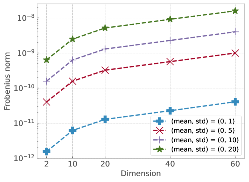
Figure 5.1: The difference measured as (5.6) of the two distance computing formulae (4.3) and (4.4) in double precision.

In general, the difference is quite minor for data from the normal distribution with mean zero and various deviations, though this difference is slightly enlarged as the standard deviation increases. Overall, the formula (4.4) should be preferred versus (4.3) in terms of computational efficiency because it enables a precomputing paradigm which avoids a great deal of repetitive computation, and therefore it will be the focus henceforth.

5.2 Cluster center update

After the selection of the $k$ initial centers, the $k$-means algorithm proceeds with updating cluster centers iteratively. In each iteration, a cluster center $\mu_{i}$ is updated by computing

$$\mu_{i}=\frac{1}{|S_{i}|}\sum_{p\in S_{i}}p,$$ (5.7)

which involves only the summation of points in the cluster $S_{i}$ and a scalar division, and thus is highly accurate, as the following lemma shows.

Lemma 5.1.

The $\mu_{i}$ computed in floating-point arithmetic is given by $\widehat{\mu}_{i}=\mu_{i}+\Delta\mu_{i}$, where $|\Delta\mu_{i}|\leq\gamma_{m_{i}}|\mu_{i}|$, $\|\Delta\mu_{i}\|\leq\gamma_{m_{i}}\|\mu_{i}\|$, where $m_{i}$ is the cardinality of the associated cluster $S_{i}$.

Proof.

The proof resembles that of Theorem 5.1 and so is omitted. ∎

We have, from Lemma 4.1 and Lemma 5.1,

$$\Delta\phi_{i}:=\phi(\widehat{\mu}_{i},S_{i})-\phi(\mu_{i},S_{i})=m_{i}\operatorname{dist}(\widehat{\mu}_{i},\mu_{i})^{2}=m_{i}\|\Delta\mu_{i}\|_{2}^{2}\lesssim m_{i}^{3}u^{2}\|\mu_{i}\|_{2}^{2},$$

where $u$ is the unit roundoff of the precision at which the center update (5.7) is carried out. This bound tells us the energy deviation associated with cluster $S_{i}$ to its minimal energy due to the presence of rounding errors. Since the dataset $\{p_{i}\}_{i=1}^{n}$ in a clustering problem is usually z-score standardized to have zero mean and unit standard deviation, $\|\mu_{i}\|_{2}$, the $2$-norm of the mean center, is expected to be close to the origin, and so the energy deviation $\Delta\phi_{i}$ should satisfy $\Delta\phi_{i}\ll 1$ if $m_{i}u\leq nu\ll 1$ holds, which is almost always true in practical applications for $u$ taken from the IEEE standard double precision or single precision.

As mentioned in the previous section, the convergence of the $k$-means algorithm relies on its property as a local improvement heuristic, that is, reassigning the data points to their closest center and then updating the cluster centers by the mean can only decrease the SSE of (4.1). For the former it is important to compute the distances accurately, which is discussed in the previous subsection, and for the latter we have the following result regarding the convergence that is most relevant towards the end of the iterations when the correction made in the center update is small.

Theorem 5.3.

Denote the computed mean centers in two successive iterations of Algorithm 4.2 as $\widehat{c}$ (the previous) and $\widehat{\mu}$ (the current), respectively. Then the convergence of the algorithm will not be terminated due to the presence of rounding errors if the unit roundoff of the precision at which the center update in Step 4 of Algorithm 4.2 is done satisfies

$$u\lesssim\frac{\left|\widehat{c}-\widehat{\mu}\right|^{T}\left|\widehat{c}-\widehat{\mu}\right|}{2\left|\widehat{c}-\widehat{\mu}\right|^{T}|\widehat{\mu}|}.$$ (5.8)

Proof.

Consider the set of points assigned to a cluster $S$ with cardinality $m$ and compare $\phi(\widehat{\mu},S)$, the energy function evaluated at the mean center of cluster $S$ computed in precision $u$, with $\phi(\widehat{c},S)$. For the convergence of $k$-means we require

$$\phi(\widehat{\mu},S)<\phi(\widehat{c},S),$$ (5.9)

which says the center update decreases the energy function.

Using Lemma 4.1 and equation (4.1), we have

$$\phi(\widehat{c},S)-\phi(\widehat{\mu},S)= \sum_{p\in S}\left(\operatorname{dist}(p,\widehat{c})^{2}-\operatorname{dist}(p,\mu+\Delta\mu)^{2}\right)$$

$$= \sum_{p\in S}\left(\operatorname{dist}(p,\widehat{c})^{2}-\operatorname{dist}(p,\mu)^{2}+2(p-\mu)^{T}\Delta\mu-\Delta\mu^{T}\Delta\mu\right)$$

$$= |S|\operatorname{dist}(\widehat{c},\mu)^{2}-2\sum_{p\in S}(\widehat{\mu}-p)^{T}\Delta\mu-m\Delta\mu^{T}\Delta\mu.$$

Using (5.7) and after some manipulation, we arrive at

$$\phi(\widehat{c},S)-\phi(\widehat{\mu},S)= m\operatorname{dist}(\widehat{c},\widehat{\mu})^{2}+2m\left(\widehat{c}-\widehat{\mu}\right)^{T}\Delta\mu-2m\Delta\mu^{T}\Delta\mu$$

$$\geq m\operatorname{dist}(\widehat{c},\widehat{\mu})^{2}-2m\left|\widehat{c}-\widehat{\mu}\right|^{T}|\Delta\mu|-2m\Delta\mu^{T}\Delta\mu,$$

which, from Lemma 5.1 and $\Delta\mu^{T}\Delta\mu=\|\Delta\mu\|_{2}^{2}\leq\gamma_{m}^{2}\|\mu\|_{2}^{2}=O(u^{2})$, implies

$$\phi(\widehat{c},S)-\phi(\widehat{\mu},S)\geq m\operatorname{dist}(\widehat{c},\widehat{\mu})^{2}-2mu\left|\widehat{c}-\widehat{\mu}\right|^{T}|\widehat{\mu}|+O(u^{2}).$$

Therefore, absorbing higher order terms in $u$, we now obtain a sufficient condition for (5.9) as

$$\operatorname{dist}(\widehat{c},\widehat{\mu})^{2}\gtrsim 2u\left|\widehat{c}-\widehat{\mu}\right|^{T}|\widehat{\mu}|,$$

where the left-hand side is the squared distance between the previous and current computed mean centers and the right-hand side accounts for the incurred rounding errors due to the floating-point computations. Rearranging the inequality completes the proof. ∎

The vector $|\widehat{\mu}-\widehat{c}|$ measures the center movement, whose norm can be large at the start of the $k$-means algorithm but tends to decrease as the iterations proceed. The precision bound (5.8) is easily computable, and it indicates that higher precision is required as the distance between the previous and next centers gets smaller, which in general happens as the iteration proceeds.

6 Mix-precision $k$-means

Algorithm 6.1 Mixed-precision $k$-means framework

Input: $P=[p_{i}]_{i=1}^{n}\in\mathbb{R}^{r\times n}$, $k$, $0<u<u_{\ell}$

1:  Call Algorithm 4.1 in precision $u_{\ell}$ to select $k$ initial centers $c_{1},\ldots,c_{k}$ from $P$, where the distance is computed by (4.4).

2:  for $c_{j}\in\{c_{1},\ldots,c_{k}\}$ do

3:     Compute $S_{j}$ centered at $c_{j}$, where the distance is computed by (4.4) in precision $u_{\ell}$.

4:     Update $c_{j}$ via (5.7) in precision $u$.

5:  end for

6:  Repeat Steps 2–5 until reaching maximum iterations or clusters set converges.

7:  Assign each $p_{i}$ to the closest cluster center $c^{j}$, i.e., $c^{j}=\operatorname*{arg\,min}_{c\in C}\|p-c\|$ computed in precision $u$, with a unique cluster label.

8:  return  $c^{1},c^{2},\ldots,c^{k}$

The goal of $k$-means algorithms is to classify all data points to their closest cluster centers, which at the beginning are chosen coarsely, via Algortihm 4.1. The subsequent iterations successively refine the positions of the centers in order to diminish the sum of squared errors SSE. From this aspect we can perform the initialization of the centers wholly in a lower-than-working precision in the mixed-precision $k$-means algorithm. Then the distance computation for finding the cluster of points associated with a center is proposed to be performed in low precision. Finally, the centers are updated via (5.7) in the working precision, which is required to satisfy the bound (5.8).

The mixed-precision $k$-means framework we propose is presented in Algorithm 6.1, where mixed precisions are used in different steps of the algorithm. Based on this framework, later we will introduce a second level of the use of mixed precisions—computing the pairwise distance in line 3 of Algorithm 6.1 in a mixed-precision fashion, and this gives the overall mixed-precision algorithm (with two different levels), presented in Algorithm 6.3.

6.1 Utilizing mixed precision in distance computation

As discussed in Section 5.1, the formula (4.4) is expected to deliver high relative accuracy when there is a great difference in the magnitude of the two vectors, despite the potential instability in evaluating the $x^{T}y$ term. This motivates our idea of exploiting mixed precision in the distance computation, which comes from the fact that in the computation of $v=z+x^{T}y$, where $|x^{T}y|\ll|z|$, the inner product $x^{T}y$ can be computed in lower precision than the subsequent addition without significantly deteriorating the overall accuracy; this idea has proven to be effective in [60], [61]. We have the following theorem which bounds the error in the mixed-precision computing scheme.

Theorem 6.1.

The squared distance $d_{r}=x^{T}x-2x^{T}y+y^{T}y$ computed in floating-point arithmetic, where $x^{T}y$ are computed in precision $u_{\ell}\geq u$ and the other parts are computed in precision $u$, satisfies $\widehat{d}_{r}=d_{r}+\Delta d_{r}$ where $|\Delta d_{r}|\lesssim(r+2)u(x^{T}x+y^{T}y)+2(r+2)u_{\ell}|x|^{T}|y|$.

Proof.

The proof is very similar to that of Theorem 5.2, and we have used the approximation $\gamma_{r}\approx ru$ in stating the result. ∎

Theorem 6.1 says that, if $\|x\|_{2}\ll\|y\|_{2}$ or $\|x\|_{2}\gg\|y\|_{2}$, we can safely compute $x^{T}y$ in precision $u_{\ell}$ chosen by

$$u_{\ell}\approx\delta u,\quad\delta:=\frac{\max\{x^{T}x,y^{T}y\}}{|x|^{T}|y|}\geq\frac{\max\{\|x\|_{2}^{2},\|y\|_{2}^{2}\}}{\|x\|_{2}\|y\|_{2}}=\max\left\{\frac{\|x\|_{2}}{\|y\|_{2}},\frac{\|y\|_{2}}{\|x\|_{2}}\right\},$$ (6.1)

such that the relative error in the computed squared distance is approximately bounded above by $3(r+2)u$, which is only three times the uniform-precision bound in Theorem 5.2.

Algorithm 6.2 Computing the distance between $p_{i}$ and a center point $c_{j}$

Input: $p_{i},c_{j}\in\mathbb{R}^{r}$, $0<u\leq u_{\ell}$, $\delta\geq 1$

1:  $s_{1}\leftarrow\|p_{i}\|_{\infty}$

2:  $s_{2}\leftarrow\|c_{j}\|_{\infty}$

3:  if condition (6.2) holds then

4:     $\widetilde{p}_{i}\leftarrow p_{i}/s_{1}$

5:     $\widetilde{c}_{j}\leftarrow c_{j}/s_{2}$

6:     Form $\mathrm{dist}(p_{i},c_{j})^{2}\leftarrow p_{i}^{T}p_{i}+c_{j}^{T}c_{j}-2s_{1}(\widetilde{p}_{i}^{T}\widetilde{c}_{j})s_{2}$, where $\widetilde{p}_{i}^{T}\widetilde{c}_{j}$ is computed in precision $u_{\ell}=\delta u$ and the rest part in precision $u$.

7:  else

8:     Form $\mathrm{dist}(p_{i},c_{j})^{2}\leftarrow p_{i}^{T}p_{i}+c_{j}^{T}c_{j}-2p_{i}^{T}c_{j}$ in precision $u$.

9:  end if

10:  return  $\mathrm{dist}(p_{i},c_{j})>0$

Putting the discussion in the context of the $k$-means algorithm, the computation of $p_{i}^{T}c_{j}$ produces the dominant term in the flop count and requires the most data communication in the distance computation, so the use of lower precisions therein can improve performance of the algorithm by both reducing flops and memory requirements (particularly the latter as vector inner product is typically a memory-bound process).

The choice of the lower precision $u_{\ell}$ should in principle follow the relation (6.1), but in practice we do not have the ability to choose an arbitrary precision, and, instead, we are more interested in the case when $u_{\ell}$ is a precision implemented in hardware. Therefore, in the $k$-means algorithm, before calculating the product $p_{i}^{T}c_{j}$ in (4.4) we check the condition (at the negligible extra cost of one scalar division)

$$\max\Big{\{}\frac{p_{i}^{T}p_{i}}{c_{j}^{T}c_{j}},\frac{c_{j}^{T}c_{j}}{p_{i}^{T}p_{i}}\Big{\}}\geq\delta^{2},\quad\delta\geq 1,$$ (6.2)

and if this condition does not hold, then the working precision will be used for the dot product $p_{i}^{T}c_{j}$; otherwise, we form the dot product $p_{i}^{T}c_{j}$ in the lower precision $u_{\ell}$. The parameter $\delta$ should be determined by $\delta\approx u_{\ell}/u$ according to (6.1), but we found that in practice this choice is very pessimistic for combinations of precision pairs $(u,u_{\ell})$ that are of practical interest. This is probably a compound effect of the fact that the bound given in Theorem 6.1 and the Cauchy–Schwarz inequality can be arbitrarily pessimistic. As a consequence, our choice for the value of $\delta$ has to become more empirical and less rigorous, making this approach difficult to be extended to employing multiple lower precisions.

Before moving to the discussion of the practical choice of $\delta$ in (6.2), we present the mixed-precision distance computing scheme in Algorithm 6.2, where we have also incorporated a trivial scaling scheme aiming to prevent overflow from the use of the low precision $u_{\ell}$, though it makes the low-precision computation be more prone to underflow.

6.2 Simulations with various $\delta$

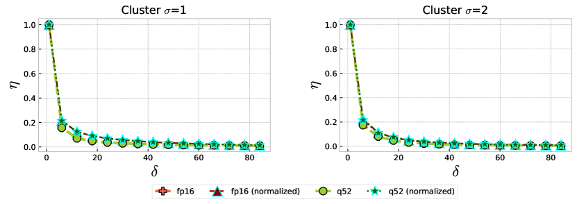
Figure 6.1: The triggered rate $\eta$ of low precision computations in terms of $\delta$ on synthetic Gaussian blobs data of different deviation $\sigma$, where 2,000 Gaussian data points with 10 clusters (blobs) are generated.

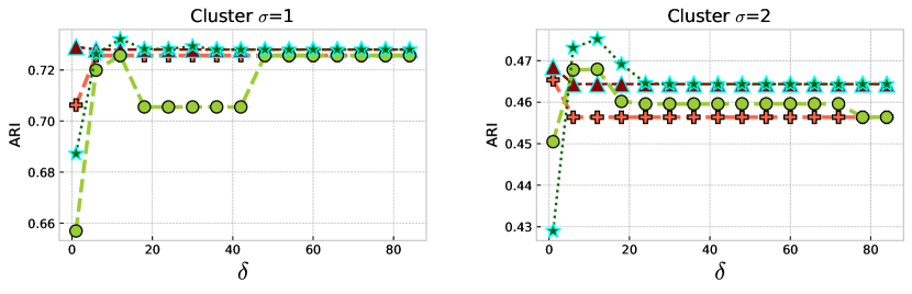
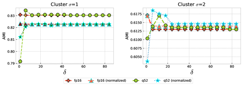
Figure 6.2: The performance in terms of ARI and AMI of Algorithm 6.3 with varying $\delta$ on on synthetic Gaussian blobs data of different deviations.

To gauge how many computations have been performed in a lower precision in computing the distance between a center and data points via Algorithm 6.2, we define and report when necessary in experiments the ratio

$$\eta=\frac{\text{The number of triggered low precision computations}}{\text{Total number of distance computations}}.$$ (6.3)

Obviously a larger chosen value for $\delta$ makes it more stringent for low precision to be used and therefore results in a reduction in the triggered rate $\eta$ of low precision computations. For $\delta=1$ the algorithm computes the distance fully in the low precision. Figure 6.1 shows that the triggering rate for low precision $\eta$ decreases as $\delta$ increases on both $z$-score normalized and nonnormalized data sets, and the triggering rate with $\delta=80$ is already close to $0$. Since the formula (6.2) is independent of data scaling, the $\eta$-$\delta$ curves on normalized and nonnormalized data sets are almost identical.

Algorithm 6.3 Mixed-precision $k$-means algorithm

Input: $P=[p_{i}]_{i=1}^{n}\in\mathbb{R}^{r\times n}$, $k$, $0<u<u_{\ell}$, $\delta\geq 1$

1:  Call Algorithm 4.1 in precision $u_{\ell}$ to select $k$ initial centers $c_{1},\ldots,c_{k}$ from $P$, where the distance $D(p)$ and $\operatorname{dist}(\cdot)$ are computed by (4.4).

2:  for $c_{j}\in\{c_{1},\ldots,c_{k}\}$ do

3:     Compute $S_{j}$ centered at $c_{j}$, where the distance is computed in specified low precision or by Algorithm 6.2.

4:     Update $c_{j}$ via (5.7) in precision $u$.

5:  end for

6:  Repeat Steps 2–5 until reaching maximum iterations or clusters set converges.

7:  Assign each $p_{i}$ to the closest cluster center $c^{j}$, i.e., $c^{j}=\operatorname*{arg\,min}_{c\in C}\|p-c\|$ computed in precision $u$, with a unique cluster label.

8:  return  $c^{1},c^{2},\ldots,c^{k}$

Also, in order to study the performance of the mixed-precision distance computation scheme, we embed this scheme into Algorithm 6.1, the mixed-precision $k$-means framework, to obtain a variant of the mixed-precision $k$-means algorithm that is presented as Algorithm 6.3. We test Algorithm 6.3 with varying $\delta$, where the working precision $u$ is double precision and the low precision is chosen as quarter precision (q52) and half precision (fp16), respectively.

The experimental results are presented in Figure 6.2. We observe that for $u_{\ell}$ being half precision (fp16), the performance of the algoirthm in terms of Adjusted Rand Index (ARI) [62] and Adjusted Mutual Information (AMI) [62] (see Section 7 for a detailed description of these measures) is quite stable as $\delta$ varies from $1$ to around $80$, showing that computing the distance in fp16 does not sacrifice the clustering quality, and in fact, the resulting quality is not much different from the algorithms with the distance computation almost fully in double precision (with $\delta=80$); we note that the AMI and ARI for double precision are almost identical to the AMI and ARI in the mixed-precision setting with $\delta=80$—as the convergence tendency of the curves shown in Figure 6.2. On the other hand, when the low precision is further reduced to be quarter precision (q52), we see that the use of the mixed-precision distance computation does bring benefits compared to the case of distance computation fully in quarter precision on both normalized and nonnormalized data.

We have further observed that the performance of the mixed-precison distance computation scheme is in general not monotonic, and in many cases a larger $\delta$ with more computation done in double precision somehow deteriorates the resulting quality. We do not have an explanation for this phenomenon, yet there is no optimal value for $\delta$ in general and its most suitable choice is clearly problem-dependent and probably also depends on the choice of precisions. From $\delta\approx 2$ the mixed precision distance computation scheme starts to achieve better or similar performance as the scheme with larger $\delta$ and more working-precision computations, and it only carries approximately half of the distance computations in the working precision (cf. Figure 6.1). Therefore, we will set $\delta=2$ in all our later experiments.

7 Numerical Experiments

In this section, we present numerical tests with the mixed-precision $k$-means algorithms. All the experiments were performed with native Python on a Linux compute server equipped with 2x Intel Xeon Silver 4114 2.2G (of a total of 20 cores, 40 threads) and 1.5 TB Random Access Memory (RAM). All algorithms are run in a single thread. Since all the $k$-means algorithms discussed in the paper invoke Algorithm 4.1 to initialize the cluster center pseudo-stochastically, we simulated five random states for the algorithms on all experiments except the image segmentation test to alleviate the effect of randomness; the segmentation test is based on cluster membership (the cluster label for each data point) and the color map is assigned based on the computed centers. The code and data to reproduce all experimental results are publicly available on GitHub. In the experiments, we will use by default double precision (fp64) as the working precision $u$ and half precision (fp16) or quarter precision (q52) as the low precision $u_{\ell}$. The lower precisions are simulated by the chop function [63]. The following algorithms are compared in the simulations.

• k-means++: the k-means++ algorithm with Algorithm 4.1 that uses (4.4) in the working precision for the distance computation.

• mp_k-means++_low: the mixed-precision k-means++ algorithm described in Algorithm 6.1 in which all the distances are computed entirely in low precision.

• mp_k-means++_mp: the mixed-precision k-means++ algorithm described in Algorithm 6.3 in which all the distances are computed via Algorithm 6.2 with $\delta=2$.

Note that both mp_k-means++_low and mp_k-means++_mp employ the mixed-precision $k$-means framework; the only difference is that mp_k-means++_low always uses the low precision in distance computation, while the low-precision distance computation in mp_k-means++_mp is triggered by Algorithm 6.2.

All tests below are performed provided ground-truth clustering numbers and labels. The performance is measured by SSE, ARI, AMI, Homogeneity, Completeness, and the V-measure [64], which we briefly review in the following:

• ARI: The Rand Index is a metric that defines the similarity between two clusterings in terms of the counting pairs assigned in the same or distinct clusters in the clustering and ground-truth clustering. Rand Index, however, tends to be larger when the two clusterings have a larger number of clusters. To fix this, the Adjusted Rand Index (ARI) is a form of Rand Index defined considering the adjustment for chance [62]. The ARI is a symmetric measure with an upper bound of 1; it has a value equal to 1 when the clusterings are identical, and close to 0 (can be negative) for random labeling independently of the number of clusters and samples.

• AMI: Mutual Information computes a measure of the mutual dependence between two clusterings. Adjusted Mutual Information (AMI) is an adjustment of the Mutual Information to account for the adjustment for chance [62]. The Adjusted Mutual Information equals 1 if two clusterings are identical and it approaches 0 (can be negative) if two random partitions are evaluated.

• Homogeneity: Homogeneity refers to all clusters of a clustering containing only data that belong to a single class such that the class distribution within each cluster has zero entropy [64], which describes the closeness of the clustering to the ground-truth clustering and ranges over $[0,1]$. When there is only a single class, homogeneity is defined to be 1.

• Completeness: Completeness refers to that all the data points that belong to a class are elements of the same cluster, it ranges from 0 to 1 [64]. The Completeness of 1 indicates a perfectly complete (successful) cluster labeling. Note that the completeness score calculated by using Scikit-learn will also be equal to $1$ when the clustering completely fails and all data points are untrained and classified to the same cluster, and, in this case, we will denote the score as NA (not applicable) to distinguish it from a perfectly perfectly complete cluster labeling.

• V-measure: It is known that Homogeneity and Completeness have an inverse relationship, i.e., Completeness is symmetrical to Homogeneity; an increasing Homogeneity often indicates a decreasing Completeness. The V-measure is computed as the harmonic mean of distinct Homogeneity and Completeness values, which can be weighted to emphasize the contributions of Homogeneity or Completeness [64].

7.1 Results for S-sets

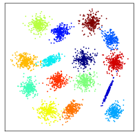
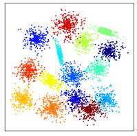
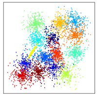
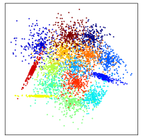
Figure 7.1: Visualization of the S-sets (colors marked as ground truth clusters).

Table 7.1: Results for the S-sets (q52).

Dataset	Metric	k-means++	k-means++ (normalized)	mp_k-means++_low	mp_k-means++_low (normalized)	mp_k-means++_mp	mp_k-means++_mp (normalized)
$S_{1}$	$\eta$	-	-	-	-	47.737 %	45.314 %;
	SSE	8.918e+12	1.546e+02	1.390e+15	6.358e+02	8.918e+12	1.756e+02
	ARI	0.98646	0.98620	0	0.70496	0.98671	0.96737
	AMI	0.98624	0.98602	0	0.85460	0.98649	0.97934
	Homogeneity	0.98633	0.98611	0	0.82629	0.98658	0.97764
	Completeness	0.98635	0.98614	NA	0.88725	0.98660	0.98138
	V-measure	0.98634	0.98612	0	0.85567	0.98659	0.97949
$S_{2}$	$\eta$	-	-	-	-	47.771 %	49.705 %
	SSE	1.563e+13	2.965e+02	7.555e+14	7.763e+02	1.511e+13	3.140e+02
	ARI	0.89039	0.89170	0	0.62097	0.88889	0.87960
	AMI	0.92854	0.92621	0	0.79057	0.92734	0.91874
	Homogeneity	0.92519	0.92240	0	0.76986	0.92415	0.91615
	Completeness	0.93298	0.93117	NA	0.81581	0.93165	0.92256
	V-measure	0.92906	0.92675	0	0.79216	0.92788	0.91934
$S_{3}$	$\eta$	-	-	-	-	47.971 %	56.856 %
	SSE	1.822e+13	4.514e+02	7.235e+14	9.212e+02	1.846e+13	4.637e+02
	ARI	0.69306	0.70628	0	0.49113	0.68548	0.70028
	AMI	0.78305	0.78732	0	0.69008	0.77971	0.78470
	Homogeneity	0.78121	0.78656	0	0.66517	0.77781	0.78405
	Completeness	0.78812	0.79123	NA	0.72201	0.78490	0.78852
	V-measure	0.78464	0.78888	0	0.69239	0.78133	0.78628
$S_{4}$	$\eta$	-	-	-	-	33.221 %	51.28 %
	SSE	1.619e+13	5.699e+02	5.964e+14	1.036e+03	1.643e+13	5.665e+02
	ARI	0.61681	0.61182	0	0.43385	0.61247	0.61716
	AMI	0.71334	0.71078	0	0.62516	0.71143	0.71239
	Homogeneity	0.71300	0.71026	0	0.60949	0.71058	0.71250
	Completeness	0.71793	0.71557	NA	0.64774	0.71655	0.71651
	V-measure	0.71544	0.71290	0	0.62796	0.71355	0.71450

Table 7.2: Results for the S-sets (fp16).

Dataset	Metric	k-means++	k-means++ (normalized)	mp_k-means++_low	mp_k-means++_low (normalized)	mp_k-means++_mp	mp_k-means++_mp (normalized)
$S_{1}$	$\eta$	-	-	-	-	47.737 %	45.223 %
	SSE	8.918e+12	1.546e+02	1.390e+15	1.547e+02	8.918e+12	1.546e+02
	ARI	0.98646	0.98620	0	0.98637	0.98671	0.98620
	AMI	0.98624	0.98602	0	0.98614	0.98649	0.98602
	Homogeneity	0.98633	0.98611	0	0.98623	0.98658	0.98611
	Completeness	0.98635	0.98614	NA	0.98625	0.98660	0.98614
	V-measure	0.98634	0.98612	0	0.98624	0.98659	0.98612
$S_{2}$	$\eta$	-	-	-	-	47.771 %	50.148 %
	SSE	1.563e+13	2.965e+02	7.555e+14	3.123e+02	1.511e+13	2.965e+02
	ARI	0.89039	0.89170	0	0.87764	0.88889	0.89170
	AMI	0.92854	0.92621	0	0.92123	0.92734	0.92621
	Homogeneity	0.92519	0.92240	0	0.91567	0.92415	0.92240
	Completeness	0.93298	0.93117	NA	0.92813	0.93165	0.93117
	V-measure	0.92906	0.92675	0	0.92181	0.92788	0.92675
$S_{3}$	$\eta$	-	-	-	-	47.971 %	56.525 %
	SSE	1.822e+13	4.514e+02	7.235e+14	4.650e+02	1.846e+13	4.730e+02
	ARI	0.69306	0.70628	0	0.69710	0.68548	0.68637
	AMI	0.78305	0.78732	0	0.78345	0.77971	0.77939
	Homogeneity	0.78121	0.78656	0	0.78170	0.77781	0.77670
	Completeness	0.78812	0.79123	NA	0.78844	0.78490	0.78541
	V-measure	0.78464	0.78888	0	0.78504	0.78133	0.78101
$S_{4}$	$\eta$	-	-	-	-	33.221 %	51.416 %
	SSE	1.619e+13	5.699e+02	5.964e+14	5.777e+02	1.643e+13	5.731e+02
	ARI	0.61681	0.61182	0	0.60722	0.61247	0.60840
	AMI	0.71334	0.71078	0	0.70933	0.71143	0.70988
	Homogeneity	0.71300	0.71026	0	0.70716	0.71058	0.70872
	Completeness	0.71793	0.71557	NA	0.71588	0.71655	0.71535
	V-measure	0.71544	0.71290	0	0.71147	0.71355	0.71202

To evaluate our mixed precision algorithms over data with clusters of various degrees of overlap, we use in this simulation the four two-dimensional datasets from [65], which are labeled and provided with ground-truth centroids with varying complexity in terms of spatial data distributions, and each dataset contains 5000 vectors and 15 clusters with a varying degree of overlap. The visualization is plotted in Figure 7.1.

The results with the low precision being fp16 or q52 are presented in Table 7.2 and Table 7.1, respectively. For nonnormalized data the SSE is naturally high in all cases, and so we should look at the other reported measures for the performance of the algorithms. We can see from the two tables that, for the normalized data, even mp_k-means++_low using fp16 achieves about the same performance as the double precision algorithm k-means++, but mp_k-means++_low completely fails on all nonnormalized data of S-sets with the low precision being fp16 or q52. On the contrary, mp_k-means++_mp achieves competing performance against the standard working-precision $k$-means algorithm with a low precision triggered rate $\eta$ of (6.3) approximately ranging from $33\%$ to $57\%$.

Comparing Table 7.2 and Table 7.1, we found mp_k-means++_mp retains similar performance with a similar low precision arithmetic triggering rate, while its benefit over mp_k-means++_low is only very clear when the low precision is set to be q52, in which case the performance of mp_k-means++_low can degrade significantly compared with the low precision being fp16; we found that this is mainly because mp_k-means++_low suffers severely from overflow problems, which is largely avoided by mp_k-means++_mp from the use of the scaling technique.

7.2 Real-world datasets

To further verify the utility and performance of the mixed-precision $k$-means algorithm on real-wolrd datasets, we evaluate the algorithms in the selected real-world datasets listed in Table 7.3. The test results with the low precision arithmetic chosen as fp16 and q52 are presented in Table 7.5 and Table 7.4, respectively.

Similarly to the results for the S-sets, we found that, with the low precision being fp16 or q52, mp_k-means++_mp also achieves competitive performance versus the standard working-precision $k$-means algorithm. On the other hand, the simulation also shows that straightforwardly executing the distance computation of the mixed-precision $k$-means framework in a low precision can fail on nonnormalized datasets or result in performance degradation on normalized datasets. Again, we see that low precision is in most cases successfully exploited by mp_k-means++_mp, and in several cases more than $70\%$ of distance computation is safely done in a much-lower-than-working precision.

Table 7.3: Summary of the real world datasets used in our test.

Dataset	Size	Dimension	Labels	Related references
Dermatology	366	34	6	[66, 67]
Ecoli	336	7	8	[66, 68, 69]
Glass	214	9	6	[66]
Iris	150	4	3	[70, 66, 71]
Phoneme	4509	256	5	[44, sect. 5]
Wine	178	13	3	[72]

Table 7.4: Results on the datasets from the UCI Machine Learning Repository (q52).

Dataset	Metric	k-means++	k-means++ (normalized)	mp_k-means++_low	mp_k-means++_low (normalized)	mp_k-means++_mp	mp_k-means++_mp (normalized)
Dermatology	$\eta$	-	-	-	-	60.612 %	46.554 %
	SSE	1.256e+04	5.616e+03	3.155e+04	6.049e+03	1.201e+04	5.731e+03
	ARI	0.06311	0.72080	0.04470	0.66875	0.04149	0.66438
	AMI	0.15150	0.85120	0.10815	0.80196	0.10599	0.81456
	Homogeneity	0.17070	0.85470	0.11070	0.78052	0.12639	0.81146
	Completeness	0.16934	0.85461	0.14507	0.83516	0.12402	0.82680
	V-measure	0.16999	0.85443	0.12489	0.80618	0.12518	0.81866
Ecoli	$\eta$	-	-	-	-	18.578 %	55.787 %
	SSE	1.481e+01	5.490e+02	6.303e+01	5.682e+02	1.586e+01	5.662e+02
	ARI	0.47399	0.47880	0.22823	0.52826	0.39939	0.47891
	AMI	0.59609	0.59621	0.22496	0.59887	0.55517	0.58445
	Homogeneity	0.69313	0.66955	0.22124	0.66107	0.66058	0.65668
	Completeness	0.54969	0.56439	0.28003	0.57542	0.50710	0.55444
	V-measure	0.61292	0.61248	0.24548	0.61516	0.57360	0.60121
Glass	$\eta$	-	-	-	-	0 %	69.188 %
	SSE	3.373e+02	8.095e+02	1.908e+03	8.036e+02	3.373e+02	8.126e+02
	ARI	0.26502	0.18333	-0.00150	0.17201	0.26502	0.18828
	AMI	0.38830	0.31508	0.00201	0.27986	0.38830	0.31873
	Homogeneity	0.38108	0.33399	0.00638	0.29823	0.38108	0.33665
	Completeness	0.45803	0.35622	0.42161	0.32593	0.45803	0.36113
	V-measure	0.41600	0.34447	0.00985	0.31068	0.41600	0.34804
Iris	$\eta$	-	-		-	22.845 %	52.518 %
	SSE	7.894e+01	1.515e+02	5.064e+02	1.543e+02	7.895e+01	1.514e+02
	ARI	0.71912	0.58906	0.09151	0.58481	0.71634	0.58817
	AMI	0.74195	0.64217	0.14595	0.64485	0.73865	0.64488
	Homogeneity	0.73943	0.63564	0.11645	0.63425	0.73642	0.63820
	Completeness	0.75099	0.66021	0.25989	0.66880	0.74749	0.66301
	V-measure	0.74516	0.64671	0.15586	0.64939	0.74191	0.64939
Phoneme	$\eta$	-	-	-	-	28.592 %	74.04 %
	SSE	5.204e+06	3.985e+05	3.196e+07	4.067e+05	5.205e+06	3.986e+05
	ARI	0.69631	0.64202	0.10937	0.59887	0.6865	0.64169
	AMI	0.73961	0.70600	0.21991	0.66569	0.73400	0.70399
	Homogeneity	0.74184	0.70857	0.14377	0.66590	0.73614	0.70661
	Completeness	0.73796	0.70409	0.52247	0.66624	0.73246	0.70204
	V-measure	0.73990	0.70632	0.22040	0.66606	0.73430	0.70432
Wine	$\eta$	-	-	-	-	57.86 %	45.644 %
	SSE	2.423e+06	1.279e+03	2.416e+07	1.289e+03	2.669e+06	1.279e+03
	ARI	0.36725	0.89407	0	0.88604	0.36282	0.89437
	AMI	0.42150	0.87536	0	0.84549	0.41517	0.87299
	Homogeneity	0.42281	0.87931	0	0.84739	0.41640	0.87721
	Completeness	0.43317	0.87403	NA	0.84683	0.42705	0.87146
	V-measure	0.42767	0.87666	0	0.84711	0.42140	0.87432

Table 7.5: Results on the datasets from the UCI Machine Learning Repository (fp16).

Dataset	Metric	k-means++	k-means++ (normalized)	mp_k-means++_low	mp_k-means++_low (normalized)	mp_k-means++_mp	mp_k-means++_mp (normalized)
Dermatology	$\eta$	-	-	-	-	60.739 %	46.777 %;
	SSE	1.256e+04	5.616e+03	1.223e+04	5.616e+03	1.256e+04	5.616e+03
	ARI	0.06311	0.72080	0.04898	0.72065	0.06311	0.72080
	AMI	0.15150	0.85120	0.12386	0.85117	0.15150	0.85120
	Homogeneity	0.17070	0.85470	0.14418	0.85470	0.17070	0.85470
	Completeness	0.16934	0.85461	0.14124	0.85454	0.16934	0.85461
	V-measure	0.16999	0.85443	0.14269	0.85440	0.16999	0.85443
Ecoli	$\eta$	-	-	-	-	19.615 %	56.021 %
	SSE	1.481e+01	5.490e+02	1.510e+01	5.490e+02	1.473e+01	5.488e+02
	ARI	0.47399	0.47880	0.43006	0.47880	0.47488	0.48045
	AMI	0.59609	0.59621	0.57679	0.59621	0.59818	0.59834
	Homogeneity	0.69313	0.66955	0.68070	0.66955	0.69530	0.67169
	Completeness	0.54969	0.56439	0.52763	0.56439	0.55153	0.56633
	V-measure	0.61292	0.61248	0.59432	0.61248	0.61491	0.61452
Glass	$\eta$	-	-	-	-	0 %	69.488 %
	SSE	3.373e+02	8.095e+02	4.933e+02	8.110e+02	3.373e+02	8.095e+02
	ARI	0.26502	0.18333	0.20581	0.18459	0.26502	0.18333
	AMI	0.38830	0.31508	0.29729	0.31697	0.38830	0.31508
	Homogeneity	0.38108	0.33399	0.24899	0.33573	0.38108	0.33399
	Completeness	0.45803	0.35622	0.47784	0.35809	0.45803	0.35622
	V-measure	0.41600	0.34447	0.32703	0.34628	0.41600	0.34447
Iris	$\eta$	-	-		-	21.684 %	52.559 %
	SSE	7.894e+01	1.515e+02	7.894e+01	1.515e+02	7.894e+01	1.515e+02
	ARI	0.71912	0.58906	0.71912	0.58906	0.71912	0.58906
	AMI	0.74195	0.64217	0.74195	0.64217	0.74195	0.64217
	Homogeneity	0.73943	0.63564	0.73943	0.63564	0.73943	0.63564
	Completeness	0.75099	0.66021	0.75099	0.66021	0.75099	0.66021
	V-measure	0.74516	0.64671	0.74516	0.64671	0.74516	0.64671
Phoneme	$\eta$	-	-	-	-	29.169 %	73.64 %
	SSE	5.204e+06	3.985e+05	2.753e+07	3.985e+05	5.204e+06	3.985e+05
	ARI	0.69631	0.64202	0.12094	0.64228	0.69631	0.64232
	AMI	0.73961	0.70600	0.29241	0.70607	0.73961	0.70624
	Homogeneity	0.74184	0.70857	0.18564	0.70864	0.74184	0.70881
	Completeness	0.73796	0.70409	0.71043	0.70416	0.73796	0.70433
	V-measure	0.73990	0.70632	0.29274	0.70639	0.73990	0.70656
Wine	$\eta$	-	-	-	-	57.592 %	45.57 %
	SSE	2.423e+06	1.279e+03	2.416e+07	1.279e+03	2.445e+06	1.279e+03
	ARI	0.36725	0.89407	0	0.89767	0.36457	0.89407
	AMI	0.42150	0.87536	0	0.87555	0.41821	0.87536
	Homogeneity	0.42281	0.87931	0	0.87976	0.41872	0.87931
	Completeness	0.43317	0.87403	NA	0.87396	0.43109	0.87403
	V-measure	0.42767	0.87666	0	0.87685	0.42443	0.87666

7.3 Image segmentation application

Figure 7.2: Tasks in images selected from ImageNet.

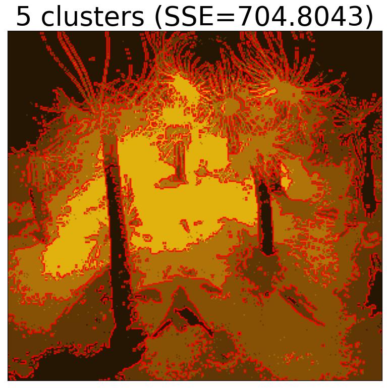
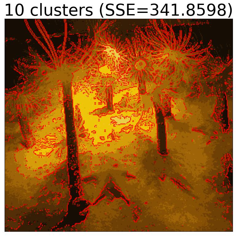
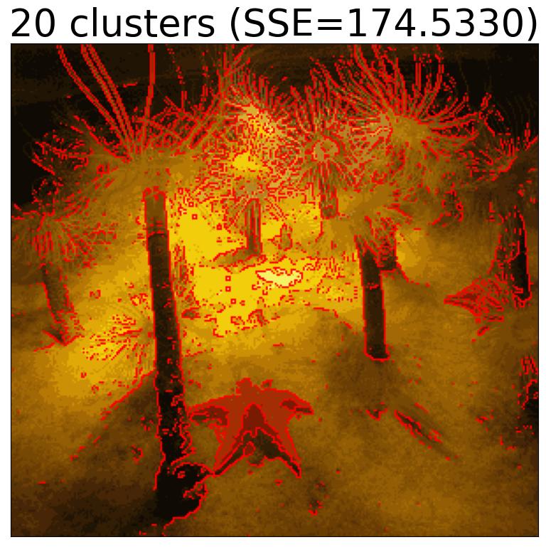
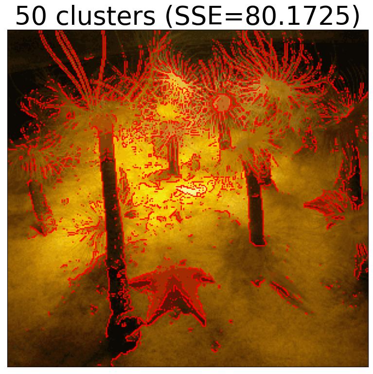
Figure 7.3: Results of image segmentation for k-means++ in the working precision (fp64).

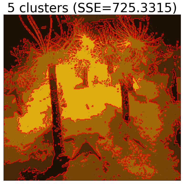
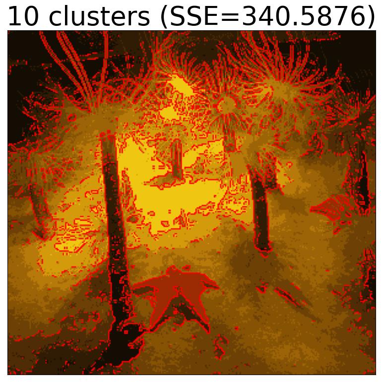
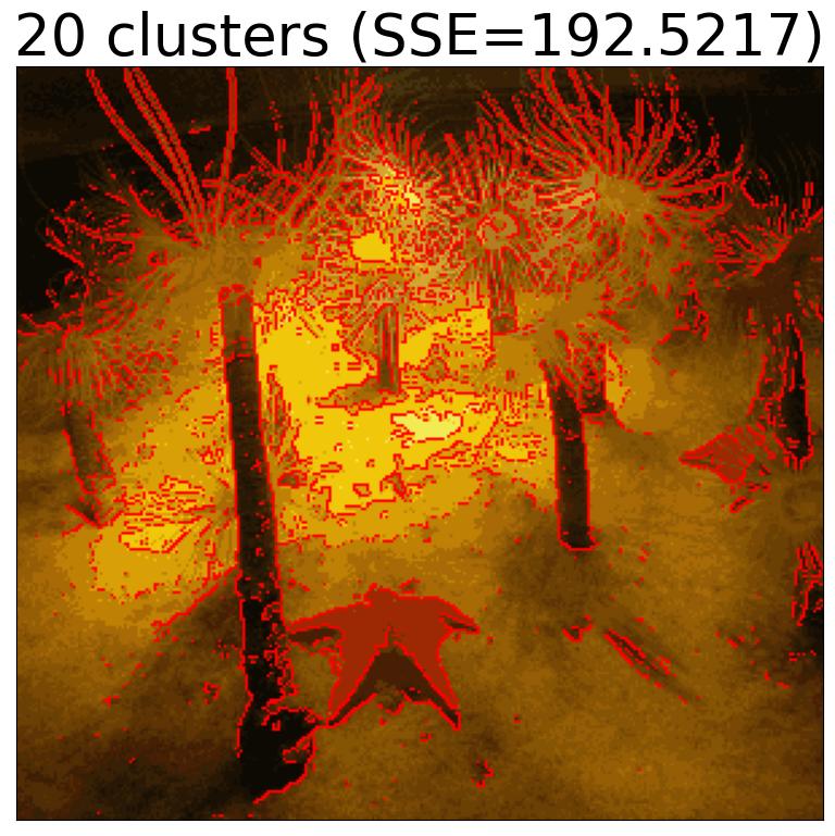
(a) mp_k-means++_low

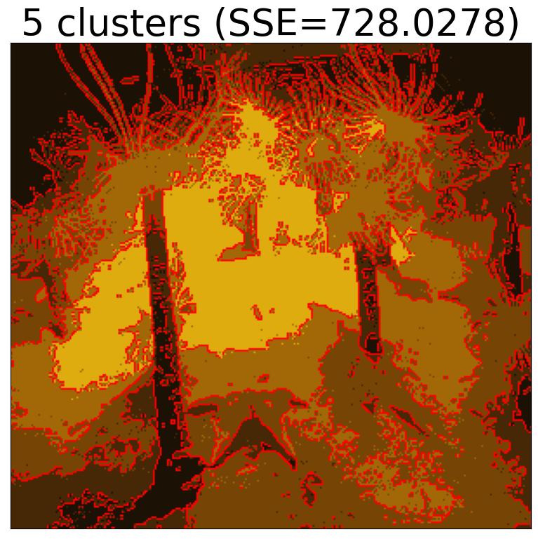
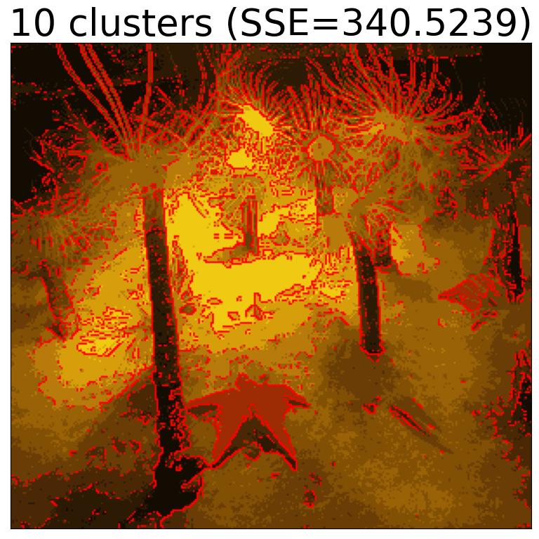
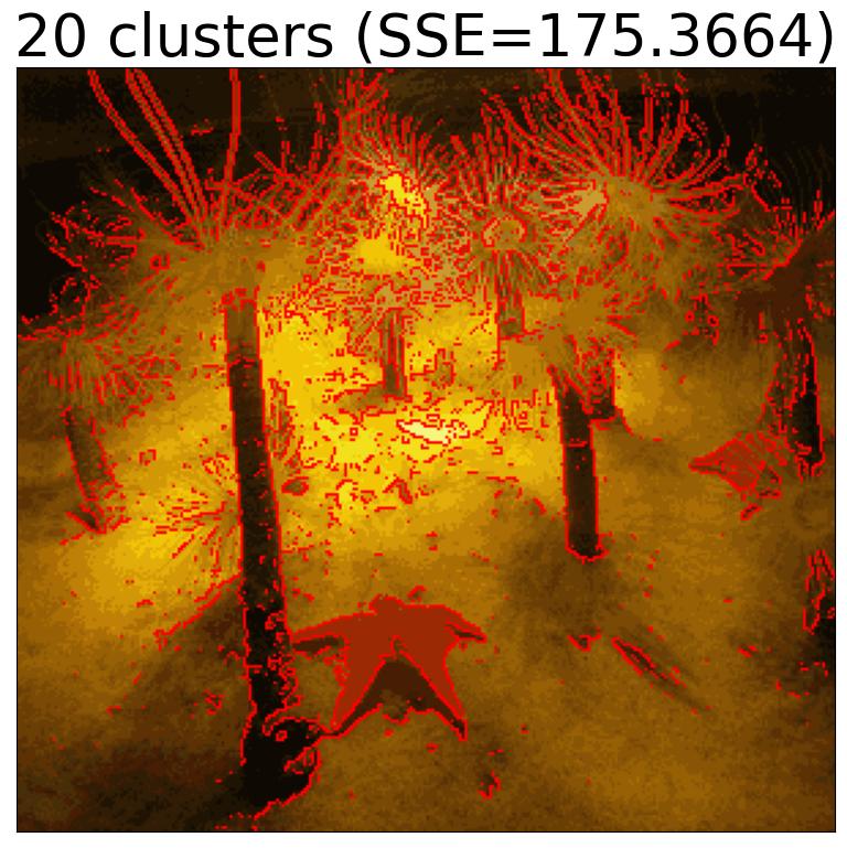
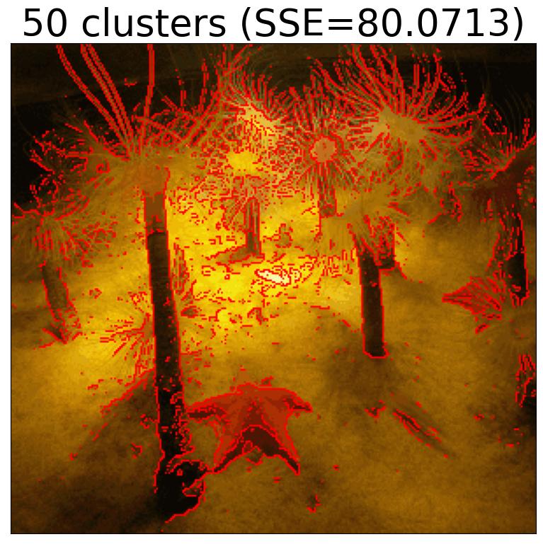
(b) mp_k-means++_mp

Figure 7.4: Results of image segmentation I (fp16).

(a) mp_k-means++_low

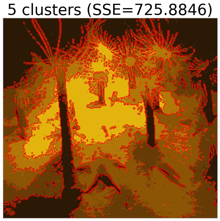
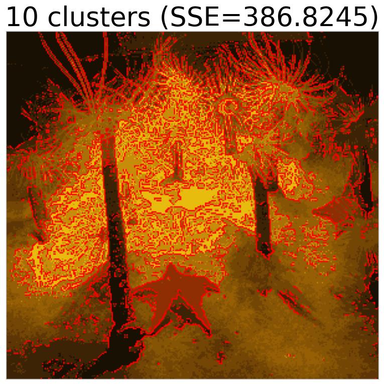
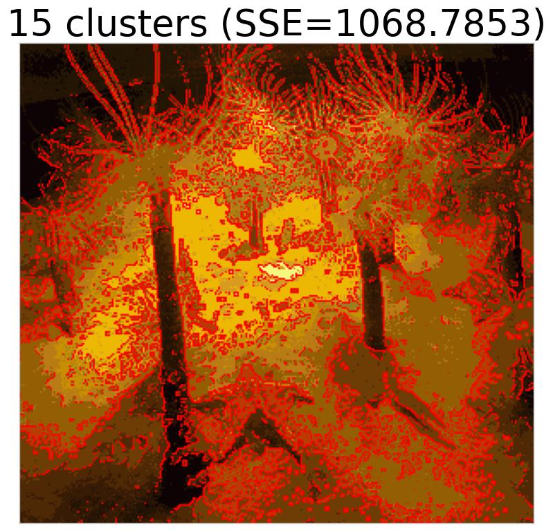
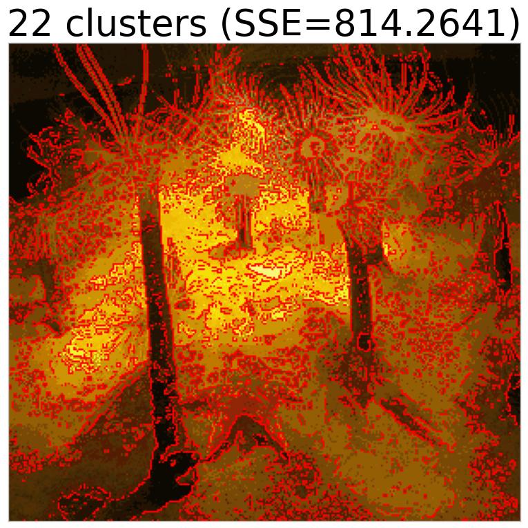
(b) mp_k-means++_mp

Figure 7.5: Results of image segmentation I (q52).

(a) mp_k-means++_low

(b) mp_k-means++_mp

Figure 7.6: Results of image segmentation II (fp16).

(a) mp_k-means++_low

(b) mp_k-means++_mp

Figure 7.7: Results of image segmentation II (q52).

We now present clustering results for an application in image segmentation for two images from ImageNet [73]. The images used for tests are as shown in Figure 7.2, where all images have been resized to be (300,280). The purpose of performing clustering in this task is to identify connected pixel regions of similar color scale in an image such that the nearby pixels (with each pixel represented as a three-dimensional vector comprised of RGB colors) tend to connect together in 2D regions in an image. Our image segmentation task follows similarly from [74].

The segmentation is completed by clustering pixels of images and the associated image is reconstructed via the cluster centers. Therefore, the reconstruction quality can be evaluated by both the perception and SSE. All data in this task is normalized by dividing each channel of the image data by 255. We evaluate k-means++, mp_k-means++_low, and mp_k-means++_mp in clusters of 5, 10, 20, and 50 and report the SSE scores.

By comparing Figure 7.3 with Figure 7.4 and Figure 7.6, we see, when various numbers of clusters are targeted and generated, the mixed-precision $k$-means algorithms, i.e., mp_k-means++_low and mp_k-means++_mp, attain an SSE score close to that obtained by the standard working precision $k$-means algorithm k-means++. When the low precision is taken to be q52, as Figure 7.5 and Figure 7.7 show, the performance of both mixed-precision $k$-means algorithms dropped significantly, particularly when the number of targeted clusters increases, though the reduction in the low precision has lesser impact on the performance of mp_k-means++_mp. Clearly, neither of the mixed-precision algorithms succeeded when the targeted number of clusters is set to be $20$ or $50$, and we found this failure is largely due to underflow in the distance computation, which resulted in a classification of many data points that are supposed to be separate in different clusters to end up in the same group.

8 Concluding remarks

In this paper we studied the numerical stability of the $k$-means method including the distance computation and center update therein, and we showed that the widely used distance computation formula is stable in floating point arithmetic. We proposed a mixed-precision framework for computing $k$-means, and, combining this framework with a new mixed-precision Euclidean distance computing scheme, we develop a mixed-precision algorithm for computing $k$-means, where the most computationally expensive part – the distance computation – is safely done in mixed precision.

We observed that the normalized data is fairly robust to the use of low precision in the distance computation, while for nonnormalized data, a reckless use of low precision often results in poor clustering performance or complete failure, which is largely due to overflow when using the low precision format. The success of Algorithm 6.3 on nonnormalized data seems to imply that underflow is often less problematic than overflow in the distance computation in $k$-means. On the other hand, we see the mixed-precision $k$-means algorithm can deliver comparable numerical results to the standard working-precision $k$-means algorithm on both normalized and nonnormalized data, typically via executing around half of the distance computations in a much lower precision (half or quarter precision), which reveals great potential for the use of mixed precision to accelerate $k$-means computations. By performing numerical simulation of low precision arithmetics on various datasets from data science tasks including data clustering and image segmentation, we showcase that appropriate reduced-precision computation for $k$-means only results in a minor increase in SSE and does not necessarily lead to worse clustering performance.

Our paper is the first attempt towards exploiting mixed precision in computing $k$-means, and, in particular, the Euclidean distance. The study may provide some insight into other Euclidean distance-based machine learning methods, e.g., data clustering [75, 56], manifold learning [76], and $k$-nearest neighbors search [77]. As it is often observed in machine learning literature that normalizing the data can somehow improve numerical precision and make it more tolerant to the reduction of precision, our study adds another such an example, though better understanding of this phenomenon in the context of Euclidean distance computation is desired. Another future research direction could be providing stronger theoretical support for the use of mixed precision in distance computation and developing a more systematic approach of low precision switching mechanism.

References

- [1] A. Gersho, R. M. Gray, Vector Quantization and Signal Compression, Springer-Verlag, New York, USA, 1991. doi:10.1007/978-1-4615-3626-0.
- [2] H. Jégou, M. Douze, C. Schmid, Product quantization for nearest neighbor search, IEEE Transactions on Pattern Analysis and Machine Intelligence 33 (1) (2010) 117–128. doi:10.1109/TPAMI.2010.57.
- [3] M. Norouzi, D. J. Fleet, Cartesian K-means, in: 2013 IEEE Conference on Computer Vision and Pattern Recognition, IEEE, 2013, pp. 3017–3024. doi:10.1109/CVPR.2013.388.
- [4] J. Jorda, A. V. Kajava, T-REKS: identification of Tandem REpeats in sequences with a K-meanS based algorithm, Bioinformatics 25 (20) (2009) 2632–2638. doi:10.1093/bioinformatics/btp482.
- [5] P. A. Marin Zapata, S. Roth, D. Schmutzler, T. Wolf, E. Manesso, D. Clevert, Self-supervised feature extraction from image time series in plant phenotyping using triplet networks, Bioinformatics 37 (6) (2020) 861–867. doi:10.1093/bioinformatics/btaa905.
- [6] J. H. Young, M. Peyton, H.-S. Kim, E. McMillan, J. D. Minna, M. A. White, E. M. Marcotte, Computational discovery of pathway-level genetic vulnerabilities in non-small-cell lung cancer, Bioinformatics 32 (9) (2016) 1373–1379. doi:10.1093/bioinformatics/btw010.
- [7] Z. Chen, Q. Sun, Extracting class activation maps from non-discriminative features as well, in: 2023 IEEE/CVF Conference on Computer Vision and Pattern Recognition, IEEE, 2023, pp. 3135–3144. doi:10.1109/CVPR52729.2023.00306.
- [8] J. Puzicha, T. Hofmann, J. M. Buhmann, Histogram clustering for unsupervised image segmentation, in: Proceedings. 1999 IEEE Computer Society Conference on Computer Vision and Pattern Recognition, IEEE, 1999, pp. 602–608. doi:10.1109/CVPR.1999.784981.
- [9] C. Zhong, Z. Sun, T. Tan, Robust 3D face recognition using learned visual codebook, in: IEEE Conference on Computer Vision and Pattern Recognition, IEEE, 2007. doi:10.1109/CVPR.2007.383279.
- [10] S. R. Gaddam, V. V. Phoha, K. S. Balagani, K-means+ID3: A novel method for supervised anomaly detection by cascading k-means clustering and ID3 decision tree learning methods, IEEE Transactions on Knowledge and Data Engineering 19 (3) (2007) 345–354. doi:10.1109/TKDE.2007.44.
- [11] S. Gupta, R. Kumar, K. Lu, B. Moseley, S. Vassilvitskii, Local search methods for k-means with outliers, Proc. VLDB Endow. 10 (7) (2017) 757–768. doi:10.14778/3067421.3067425.
- [12] C. Ordonez, E. Omiecinski, Efficient disk-based k-means clustering for relational databases, IEEE Transactions on Knowledge and Data Engineering 16 (8) (2004) 909–921. doi:10.1109/TKDE.2004.25.
- [13] S. Wang, Y. Sun, Z. Bao, On the efficiency of K-means clustering: Evaluation, optimization, and algorithm selection, Proc. VLDB Endow. 14 (2) (2020) 163–175. doi:10.14778/3425879.3425887.
- [14] S. Guo, N. Yao, Document vector extension for documents classification, IEEE Transactions on Knowledge and Data Engineering 33 (8) (2021) 3062–3074. doi:10.1109/TKDE.2019.2961343.
- [15] D. Arthur, S. Vassilvitskii, How slow is the k-means method?, in: SCG’06: Proceedings of the 22nd annual symposium on Computational geometry, ACM Press, New York, USA, 2006, pp. 144–153. doi:10.1145/1137856.1137880.
-
[16]
D. Arthur, S. Vassilvitskii,