Tool Shape Optimization through Backpropagation of Neural Network
Abstract
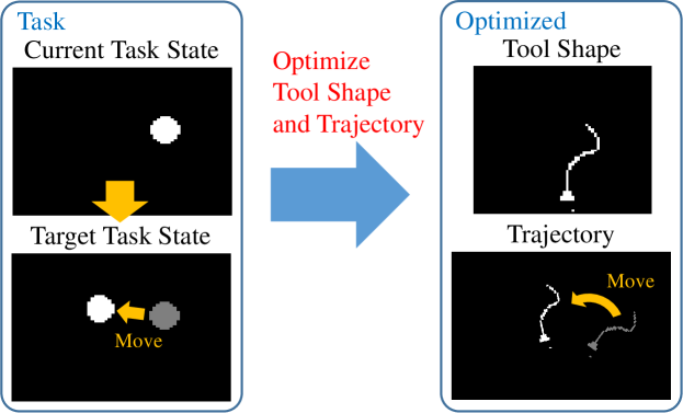
When executing a certain task, human beings can choose or make an appropriate tool to achieve the task. This research especially addresses the optimization of tool shape for robotic tool-use. We propose a method in which a robot obtains an optimized tool shape, tool trajectory, or both, depending on a given task. The feature of our method is that a transition of the task state when the robot moves a certain tool along a certain trajectory is represented by a deep neural network. We applied this method to object manipulation tasks on a 2D plane, and verified that appropriate tool shapes are generated by using this novel method.
I INTRODUCTION
Tool-use is one of the fundamental abilities of human beings. When executing a task, human beings can choose or make an appropriate tool to achieve the task. For a robot to work in a human environment, combining existing tools or making new tools is necessary to expand its capability. In this study, we mainly focus on the optimization of tool shape and tool trajectory, as a foundation of tool making.
Robotic tool-use has been studied in various topics: tool recognition [1, 2], tool understanding [3, 4], tool choice [5, 6], and motion generation with tool-use [7, 8, 9]. However, there have been few studies about tool-making or making a new appropriate tool for a given task. Nair, et al. developed methods to construct a new tool by combining two existing tools using geometric reasoning [10, 11]. Wicaksono, et al. developed frameworks of tool creation as an extension of tool-use learning [12, 13]. However, because [10, 11] can generate only tools expressed by the combination of two existing tools and [12, 13] can generate only tools similar to a reference tool due to random generation of tools fulfilling many hypotheses (e.g. a hook-like tool), various free forms of tool shapes cannot be handled. Also, because [12, 13] must be tested by the actual robot to choose the best tool, the optimization of tool shape takes too much time.
Apart from robotic tool-use, an optimization method of robot design parameters such as link length and actuator placement has been developed [14]. Also, some studies have jointly optimized the robot design parameters and control scheme using a genetic algorithm [15, 16] or reinforcement learning [17], in simulation environment. While these studies are similar to the scenario of tool making, there are two problems in common. First, these robot designs (e.g. link length and actuator placement) are manually parameterized and various free forms cannot be handled. To appropriately parameterize the design, prior knowledge of human experts is necessary. Second, experiments of almost all previous works are conducted in simulation environment. This is because we must move the robot to obtain evaluation value in the process of optimization and it takes too much time in the actual environment. Also, these studies cannot consider the characteristics of the actual environment, e.g. friction, hysteresis, and robot model error.
Our contributions of this study are as below,
-
•
We use an image to represent a tool shape. A tool shape can be easily converted to an image, and we can uniformly handle various tool shapes without prior knowledge.
-
•
All experiments including evaluations are conducted in the actual environment. By acquiring a tool-use model using the actual robot data of random movements, the tool shape is directly optimized without evaluating the movements of the actual robot.
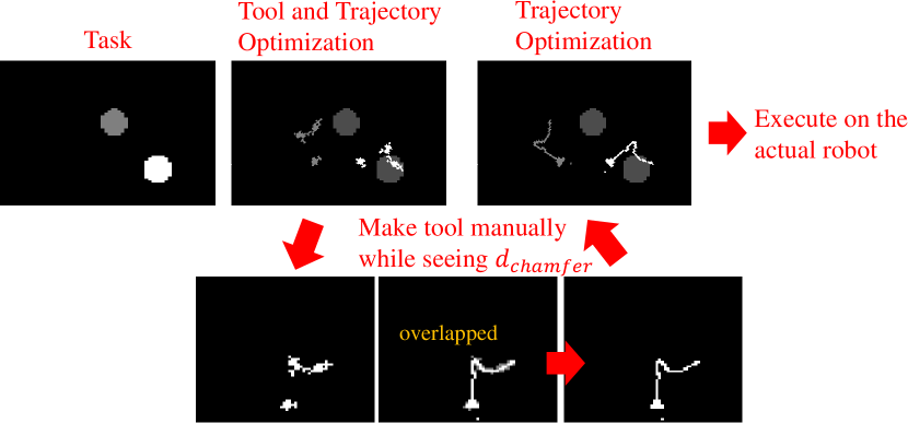
As shown in Fig. 1, this study simultaneously calculates an optimized tool shape and trajectory for a given task. A transition of the task state when a robot moves a certain tool along a certain trajectory is represented by a deep neural network. An optimized tool shape, tool trajectory, or both for a target task, can be obtained by using the backpropagation technique [18] of the neural network. Although this method includes motion trajectory optimization, we mainly put stress on tool shape optimization. We conduct experiments using the actual robot on a 2D plane to verify the effectiveness of this study.
II Tool Shape and Trajectory Optimization Network
In this study, we represent a transition of task state, when using a given tool shape and trajectory, by a neural network. We call this network “Tool Shape and Trajectory Optimization Network (Tool-Net)”.
In the following sections, we assume that the robot moves on a 2D plane and the task is an object manipulation task, for simplicity. In Section IV, we will discuss extensions of our method to a robot that moves in 3D space and other kinds of tasks.
II-A Network Structure of Tool-Net
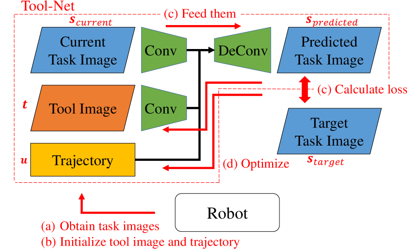
The network structure of Tool-Net is shown in Fig. 2. This network is represented by the equation below,
| (1) |
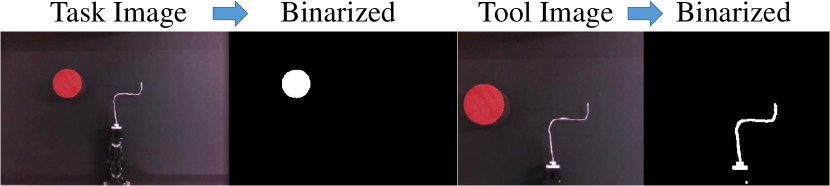
where is a current task state, is a tool shape, is a tool trajectory, is a predicted task state after moving the robot using and , and represents Tool-Net. is trained, and and are optimized when given a target task state . Because we handle object manipulation tasks in this study, we use a binarized image as shown in Fig. 1, which can flexibly express the object position and posture, as task state . We also use a binarized image, which has high degrees of freedom, as tool image . In binarized images, the background color is black (its value is 0), and the tool and manipulated object color is white (its value is 1). Regarding tool trajectory, we assume quasi-static movement and constant joint velocity in this study, and so we represent as . is the starting or ending joint angles of the robot, and the whole trajectory is the trajectory that interpolates these joint angles linearly by constant velocity.
In detail, and are inputted through convolutional layers and concatenated with , and is outputted through deconvolutional layers.
II-B Data Collection for Tool-Net
The procedures to collect data for training of Tool-Net are as below.
-
(a)
Initialize the robot posture and attach a randomly generated tool to the manipulator tip
-
(b)
Obtain the tool shape image
-
(c)
Set randomly and move the robot
-
(d)
Randomly place an object
-
(e)
Obtain the task state image
-
(f)
Set randomly and move the robot
-
(g)
Obtain the task state image
-
(h)
Repeat (c) – (g), collect the data, and go back to (a) after the conditions (described below) are satisfied
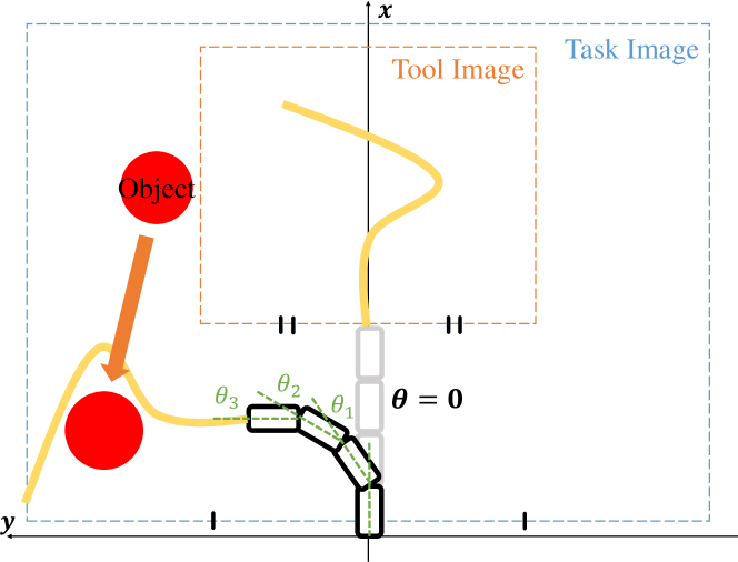
In (a), the joint angle of the robot is initialized to . We define the joint angles as shown in Fig. 3, and so the initialized posture is straightly aligned. To prepare various tool shapes to be attached to the robot, we make tools randomly by hand with a metal wire, which will be explained in Section III-A. 3D printing or clay modeling are also applicable for the purpose.
In (c) and (f), when the robot is randomly moved, the limit of is set ( is the lower or upper limit of joint angles). Also, because the robot hardly moves when is close to , we set the limit of when randomly choosing the ( expresses L1 norm).
In (h), we use a sampling technique to balance changed samples and unchanged samples. A changed sample means that the robot moves the target object, and an unchanged sample means that the robot does not touch the target object. Due to the random trajectory, we get more unchanged samples than changed samples. We use symmetric chamfer distance [19] to distinguish changed or unchanged samples as below,
| (2) |
where , are images with the same size, DT (Distance Transform) is an image expressing the distance to the nearest white pixel at each pixel, and the unit of is [px]. When , it is classified as a changed sample. For each tool, we collect changed samples and unchanged samples into a dataset ( is the number of samples). After obtaining all these data, we go back to procedure (a) with a new tool. By repeating these procedures, we finally construct a dataset for the training of Tool-Net.
When constructing a dataset, we augment it at the same time. When executing the procedures (c) – (g), we collect not only (, , , ) but also and at all frames. Then, we randomly choose frame indices () from the consecutively collected data, and add data (, , , ) into the dataset ( is the number of the data). is or at the frame of or . When defining the arrangement of the robot and task image as shown in Fig. 3, we can also generate a mirrored data of (, , , ) (Mirror expresses a mirrored image). Therefore, we finally obtain data: (, , , ).
In our experiments, we set [deg], [deg] regarding each actuator, [deg], [px], , , and .
II-C Training Phase of Tool-Net
We preprocess the obtained dataset (, , , ) and train Tool-Net. This preprocess makes the training result robust against noise and displacement of pixels.
First, we augment tool image data by adding noise. We show how to add noise in Alg. 1.
In Alg. 1, is the function which randomly extracts one pixel from . is the function which counts the number of white pixels among 4 adjacent pixels to the of . is the function which makes the of {white, black}. is the function which judges whether the in is {white, black}. is with noise. , are constant values. Line 4–11 of Alg. 1 express that we randomly make the black pixel white when its adjacent pixels include at least one white pixel. Line 12–18 of Alg. 1 express that we randomly make the white pixel black.
Second, to make Tool-Net robust against the displacement of pixels, we blur the task state image , as shown below,
| (3) |
where is a constant value. The smaller is, the more the image is blurred.
Using and , we train Tool-Net with the loss shown below, by setting the number of epochs as and batch size as ,
| (4) | ||||
| (5) |
where MSE expresses mean squared error.
In the following experiments, we set , , , , and .
II-D Optimization Phase of Tool-Net
We will explain the optimization procedures of tool shape and trajectory using trained Tool-Net. The procedures corresponding to Fig. 2 are as below.
-
(a)
Obtain the current task state and target task state
-
(b)
Generate the initial tool shape and trajectory before optimization
-
(c)
Calculate loss of
-
(d)
Update through backpropagation
-
(e)
Repeat (c) and (d) times
In (b), regarding , we randomly extract tools from the dataset constructed in Section II-B ( is the number of the batch), and apply AddNoiseToTool in Alg. 1 to each tool. Regarding , we randomly generate tool trajectories fulfilling the limit of . Thus, we construct a batch with samples of and .
In (c), we calculate regarding each data in the batch ( is blurred by Eq. 3).
In (d), we backpropagate and optimize and for each data. First, regarding the optimization of tool trajectory, we optimize like in [20, 21], as below,
| (6) |
where expresses L2 norm, and is an update rate.
Second, regarding the optimization of tool shape, we change the values of pixels according to the gradient . To decrease , the black pixels with negative gradients should be changed to white, and the white pixels with positive gradients should be changed to black. However, if all pixels are changed according to the gradient, an appropriate image for tool shape cannot be obtained due to sporadic pixels. Also, white pixels sometimes concentrate in small areas. To solve these problems, we optimize tool shape by focusing on adjacent pixels, as shown in Alg. 2.
In Alg. 2, is the function which judges whether the gradient of is {positive, negative}. is the function which extracts of . is the function which extracts values in from {front, back} of the array. , , , and are constant values. We calculate a score for each pixel from the gradient and the number of adjacent white pixels. In ascending order of this score, the top and the bottom pixels are turned to white and black, respectively. is updated by in Alg. 2.
After iterations of Eq. 6 and , candidates of tool shapes and trajectories are obtained. We use the tool shape and trajectory with minimum among all candidates as the optimized value of and .
We explained the method of optimizing both tool shape and trajectory at the same time. In the case that either tool shape or trajectory is optimized, the other is fixed and not optimized. In the following experiments, we set , , [rad], , , , and .
II-E Detailed Implementation
The image binarization procedures of and are Crop, Color Extraction, Closing, Opening, and Resize, in order. Color Extraction separates the input image into tool, object, and background images. To make this process easy, we use a silver tool and the object is colored red. Note that the robot arm is considered as a background. Crop is executed as in Fig. 3, and Resize converts the image to the size of 6464.
The convolutional layers for and have the same structures. Each of them has 6 layers, and the number of each channel is 1 (input), 4, 8, 16, 32, and 64. Its kernel size is 33, stride is 22, padding is 1, and batch normalization [22] is applied after each layer. and are compressed to a 128 dimensional vector by fully connected layers, it is concatenated with , and a dimensional vector is generated ( is the number of actuators of the robot). After that, the vector is fed into fully connected layers whose numbers of units are , 128, 128, 128, and 256. The deconvolutional layers have the same structure with the convolutional layers, but only the last deconvolutional layer does not include batch normalization. The activation function of the last deconvolutional layer is Sigmoid, and those functions of the other layers are ReLU.
III Experiments
We will explain our experiments using the actual robot: the training of Tool-Net, the optimization of tool shapes using Tool-Net, and evaluation of the optimized tools. Also, we will show an advanced application of tool shape optimization for multiple tasks.
III-A Experimental Setup
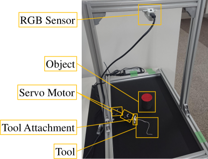
We show the experimental setup of this study in Fig. 4. Aluminum frames are structured on a black background sheet, and a camera and manipulator with 2 servo motors are attached to the structure. The servo motors are Dynamixel Motor (XM430-W350-R), and the camera is D435 (Intel Realsense). As a tool, we used metal wire with a diameter of 3 mm, which has enough strength for object manipulation tasks and can be bent by hand. A mount to attach the tool to is equipped at the tip of the manipulator. The object for the manipulation task is a cylinder-shaped wooden block painted red for color extraction.
We show the images binarized by the method of Section II-E in the left figure of Fig. 5. The tool shape and task state are extracted and binarized as shown in the right figure of Fig. 5, and we use them for Tool-Net after resizing.
III-B Tool Shape and Trajectory Optimization for One Task
III-B1 Training Phase
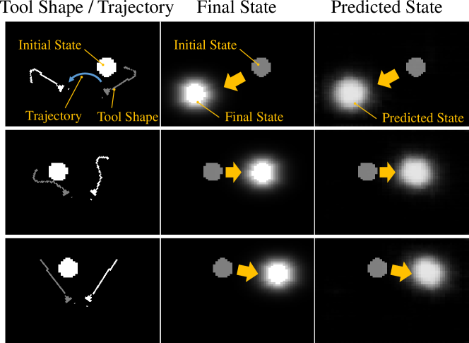
We conducted data collection procedures for 48 kinds of tools over 2 hours in total, and obtained 36000 number of data. We trained Tool-Net using these data by epoch, and used the model with minimum . We show the prediction results of task state in Fig. 6. When given a certain tool shape and trajectory, Tool-Net was able to predict the transition of task state correctly. We drew the tool trajectory by solving forward kinematics of the robot.
III-B2 Optimization Phase
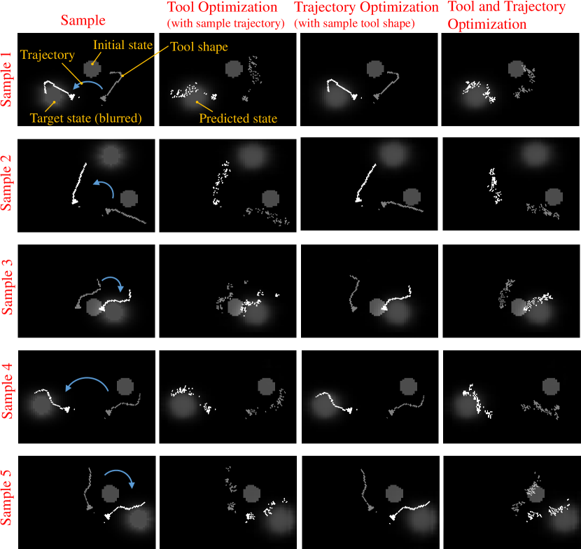
We prepared Sample 1 – 5 with the data of . As we set and , we compared three optimizations: optimization of only tool shape, only tool trajectory, and both. When optimizing only tool shape, the tool trajectory is fixed to , and when optimizing only tool trajectory, the tool shape is fixed to . Note that the sample data is just for reference and is not used for optimization except for the fixed trajectory or tool shape. We show the optimization results in Fig. 7. The left column shows sample data and the remaining three columns show the three optimization results. Although this optimization phase depends on the initial value, when is large (e.g. ), almost the same results are obtained in every trial.
Even though the tool shape is initialized by randomly chosen data from the training dataset and the tool trajectory is initialized by random values as explained in Section II-D, and indicate almost the same position and so the optimization succeeds. represents the predicted state when using the optimized tool shape and trajectory. For example, regarding Sample 1, a different tool shape from the sample data is generated, and it is reasonable for the task because it wraps the object well. Regarding Sample 2, a tool shape like the sample data is generated. Regarding the tool shape and trajectory optimization of Sample 3, a tool shape without the parts of the sample data, which do not contribute to the manipulation, is generated. We can see that various kinds of tool shapes are generated, not just the same shape with the sample data.
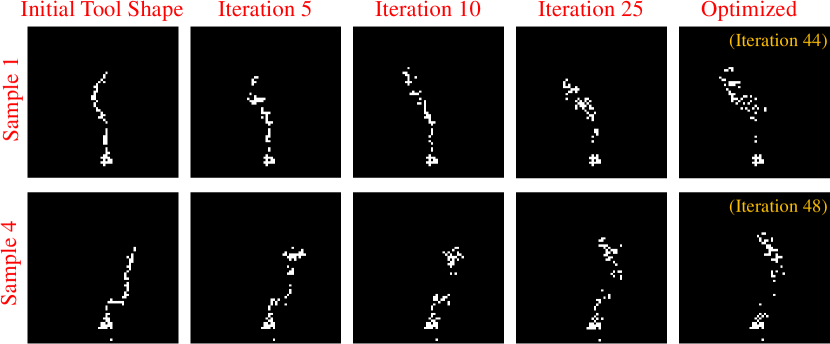
Regarding the tool shape optimization of Sample 1 and 4, we show the transition of tool shape according to the iteration of optimization in Fig. 8. In actuality, although we start optimization from initial tool shapes and choose the best one, we show only the transition of tool shape regarding the best tool finally chosen. As we can see from the initial tool shape, the optimization starts from the tool shape that is close to the final shape, and it gradually changes.
III-B3 Evaluation of Optimization Phase
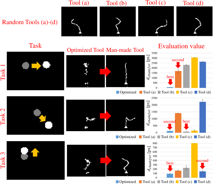
Regarding the tool shape and trajectory optimization, we evaluated the degrees of task realization in an actual robot experiment. We prepared Task 1 – 3 with the data of . By the procedures shown in Fig. 9, the task is executed with the optimized tool, and task realization is evaluated. First, the tool shape and trajectory are optimized at the same time for the given task. Second, the optimized tool shape is made with metal wire by human hands. When between optimized and current tool shapes becomes lower than 150 px, it is regarded that the same tool shape is made. Although this procedure includes some human arbitrariness, the threshold was enough to resemble the generated tool in this experiment. Third, only the tool trajectory is optimized for the man-made tool, and the optimized motion is executed. After the task execution, between the final task state and the target task state is measured. We repeated the procedures from task execution to measurement of 5 times, and calculated its average and variance. Also, we prepared 4 random tool shapes: Tool (a) – (d), for comparison as shown in the upper figure of Fig. 10. Regarding each random tool, only the tool trajectory is optimized, the optimized motion is executed, and the average and variance of are calculated.
Regarding each task, we show the task, optimized tool shape, man-made tool shape based on the optimized one, and the average and variance of , in Fig. 10. From the average of , we can say that the degrees of task realization depend on the tool shapes, and they are high in general when using the optimized tools. Regarding Task 1, in which the object is placed far from the robot, the optimized tool is straight-shaped and can achieve the task well, where Tool (a) – (d) cannot reach the object. Regarding Task 2, the tool shapes of Tool (b), (c) and the optimized one have the same shape to wrap and pull the object to the right front side, and the are almost the same.
III-C Tool Shape Optimization for Multiple Tasks
The optimization of tool shape in this study has a potential to be applied for not only one task but also multiple tasks. This can be executed by summing up obtained for multiple tasks and backpropagating it.
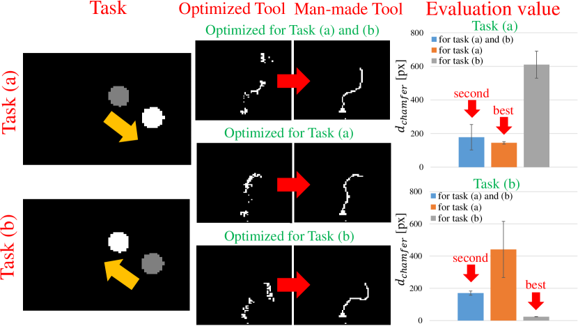
To evaluate the applicability for multiple tasks, we prepared reversed tasks, Task (a): and Task (b): . We executed experiments of the tool shape and trajectory optimization for only Task (a), only Task (b), and both, like in Section III-B3, and then, calculated the average and variance of between the final task state and the target task state. We show the results in Fig. 11. The tool shape optimized for either Task (a) or (b) has a shape to wrap the object firmly. On the other hand, the tool shape optimized for both Task (a) and (b) has a shape with a gentle curve, and can be used for both Task (a) and (b). Regarding , when using the optimized tool shape for only Task (a), Task (a) is realized well, but Task (b) cannot be realized. On the other hand, when using the optimized tool shape for both Task (a) and (b), both tasks can be realized to some extent.
IV Discussion
IV-A Experimental Results
The experimental results in Section III-B1 indicate that Tool-Net can infer the change of task state from the current task state, tool shape, and tool trajectory. Section III-B2 demonstrates that various tool shapes and tool trajectories are generated as a result of the optimization process. These tool shapes are usually reasonable, because they wrap the target object well, have no useless parts that do not contribute to the manipulation, etc. However, their pixels lose continuity. In Section III-B3, humans made the optimized tool shape by hand while referencing , and the optimized trajectory was executed. As a result, the optimized tool shapes can achieve the target tasks better than the randomly generated tool shapes. While the randomly generated tools usually cannot reach the target object or cannot wrap the object well, the optimized tools can reach and wrap it well. In Section III-C, Tool-Net is also applicable to multiple tasks. While a tool optimized for a certain task can realize the task well, the tool shape is hard to be used for other tasks. In contrast, while a tool optimized for multiple tasks is a little inferior to the tools optimized for each task, the tool shape has versatility that can be used for the multiple tasks.
Our system has a problem on the making of actual tools, because the generated tool shapes lose continuity of pixels and cannot be directly made. Because humans make a tool similar to the optimized one while referencing in this study, this process depends on human interpretation. To solve the problem, we need to develop techniques of generating realizable tool shapes while keeping the diversity of tool shapes.
IV-B Future Directions
We believe that this framework can be applied to not only object manipulation but also more general tasks, by changing the definition of task state. For example, by using 6 axis force sensor or frequency and amplitude of sound as the task state, a force applying or sound making task could be achieved.
Because the metal wire is used for experiments, the generated tool shape is limited to the shape drawn by one stroke. This spoils the benefits of using the binarized image as tool expression. If we can use 3D printer or clay for tool-making, the benefits of using an image can be emphasized more, because tool shapes with branches and larger areas can be handled.
Tool material or friction coefficient also sometimes affects task execution. Although a binarized image cannot express these characteristics, we may be able to optimize tool shape considering them by embedding this information into an image with multiple channels like color image.
If we would like to handle 3D movement, by using 3D voxel representation with depth image for tool shape, we believe this study could be extended to the 3D movement.
This framework could be also applicable to the flexible manipulator, if the representation of tool trajectory is changed by adding time information to or making the network a recurrent one. Such networks will have a similar structure with [20].
We came up with this study when seeing a human drop a key into a gutter by mistake and pick it up using metal wire. To achieve this task, not only the expansion to 3D movement, but also a consideration of obstacles and efficient learning will be required. In the current form, the necessary number of trials explodes exponentially depending on the number of robot actuators and degrees of freedom of tool shape representation. It will be important for efficient training of Tool-Net to address the curse of dimensionality by using not only obtained data but also prior knowledge such as physical laws and the analogy of own body and tool shape like in [6].
V CONCLUSION
We proposed a method to obtain an optimized tool shape and trajectory for given tasks using backpropagation technique of a neural network. A transition network of task state by a certain tool shape and trajectory is trained, and a tool shape and trajectory to realize the target task state are calculated using it. Also, we proposed data augmentation for efficient training, and a method to update pixels in tool shape image for optimization. Finally, the given tasks can be achieved more accurately by using the optimized tool shape. In future works, by using not only obtained data but also prior knowledge such as physical laws and robot configuration, we will expand this method to a more practical form.
References
- [1] E. Huber and K. Baker, “Using a hybrid of silhouette and range templates for real-time pose estimation,” in Proceedings of the 2004 IEEE International Conference on Robotics and Automation, 2004, pp. 1652–1657.
- [2] C. C. Kemp and A. Edsinger, “Robot manipulation of human tools: Autonomous detection and control of task relevant features,” in Proceeding of the 2006 International Conference on Development and Learning, 2006, pp. 1–6.
- [3] Y. Zhu, Y. Zhao, and S. Zhu, “Understanding tools: Task-oriented object modeling, learning and recognition,” in Proceedings of the 2015 IEEE/CVF International Conference on Computer Vision and Pattern Recognition, 2015, pp. 2855–2864.
- [4] A. Myers, C. L. Teo, C. Fermüller, and Y. Aloimonos, “Affordance detection of tool parts from geometric features,” in Proceedings of the 2015 IEEE International Conference on Robotics and Automation, 2015, pp. 1374–1381.
- [5] N. Saito, K. Kim, S. Murata, T. Ogata, and S. Sugano, “Tool-Use Model Considering Tool Selection by a Robot Using Deep Learning,” in Proceedings of the 2018 IEEE-RAS International Conference on Humanoid Robots, 2018, pp. 270–276.
- [6] K. P. Tee, J. Li, L. T. P. Chen, K. W. Wan, and G. Ganesh, “Towards Emergence of Tool Use in Robots: Automatic Tool Recognition and Use Without Prior Tool Learning,” in Proceedings of the 2018 IEEE International Conference on Robotics and Automation, 2018, pp. 6439–6446.
- [7] K. Okada, M. Kojima, Y. Sagawa, T. Ichino, K. Sato, and M. Inaba, “Vision based behavior verification system of humanoid robot for daily environment tasks,” in Proceedings of the 2006 IEEE-RAS International Conference on Humanoid Robots, 2006, pp. 7–12.
- [8] M. Toussaint, K. Allen, K. Smith, and J. Tenenbaum, “Differentiable Physics and Stable Modes for Tool-Use and Manipulation Planning,” in Proceedings of the 2018 Robotics: Science and Systems, 2018.
- [9] K. Fang, Y. Zhu, A. Garg, A. Kurenkov, V. Mehta, L. Fei-Fei, and S. Savarese, “Learning Task-Oriented Grasping for Tool Manipulation with Simulated Self-Supervision,” in Proceedings of the 2018 Robotics: Science and Systems, 2018.
- [10] L. Nair, J. Balloch, and S. Chernova, “Tool Macgyvering: Tool Construction Using Geometric Reasoning,” in Proceedings of the 2019 IEEE International Conference on Robotics and Automation, 2019, pp. 5837–5843.
- [11] L. Nair, J. Balloch, and S. Chernova, “Autonomous Tool Construction Using Part Shape and Attachment Prediction,” in Proceedings of the 2019 Robotics: Science and Systems, 2019.
- [12] H. Wicaksono and C. Sammut, “A Learning Framework for Tool Creation by a Robot,” in Proceedings of the 2015 Australasian Conference on Robotics and Automation, 2015.
- [13] H. Wicaksono, C. Sammut, and R. Sheh, “Towards Explainable Tool Creation by a Robot,” in Proceedings of International Joint Conference on Artificial Intelligence - Workshop on Explainable AI (XAI), 2017.
- [14] S. Ha, S. Coros, A. Alspach, J. Kim, and K. Yamane, “Joint Optimization of Robot Design and Motion Parameters using the Implicit Function Theorem,” in Proceedings of the 2017 Robotics: Science and Systems, 2017.
- [15] K. Sims, “Evolving Virtual Creatures,” in Proceedings of the 21st Annual Conference on Computer Graphics and Interactive Techniques, 1994, pp. 15–22.
- [16] H. Lipson and J. Pollack, “Automatic design and manufacture of robotic lifeforms,” Nature, vol. 406, no. 6799, pp. 974–978, 2000.
- [17] C. Schaff, D. Yunis, A. Chakrabarti, and M. R. Walter, “Jointly Learning to Construct and Control Agents using Deep Reinforcement Learning,” in Proceedings of the 2019 IEEE International Conference on Robotics and Automation, 2019, pp. 9798–9805.
- [18] D. E. Rumelhart, G. E. Hinton, and R. J. Williams, “Learning representations by back-propagating errors,” nature, vol. 323, no. 6088, pp. 533–536, 1986.
- [19] G. Borgefors, “Hierarchical chamfer matching: a parametric edge matching algorithm,” IEEE Transactions on Pattern Analysis and Machine Intelligence, vol. 10, no. 6, pp. 849–865, 1988.
- [20] K. Kawaharazuka, T. Ogawa, J. Tamura, and C. Nabeshima, “Dynamic Manipulation of Flexible Objects with Torque Sequence Using a Deep Neural Network,” in Proceedings of the 2019 IEEE International Conference on Robotics and Automation, 2019, pp. 2139–2145.
- [21] K. Kawaharazuka, T. Ogawa, and C. Nabeshima, “Dynamic Task Control Method of a Flexible Manipulator Using a Deep Recurrent Neural Network,” in Proceedings of the 2019 IEEE/RSJ International Conference on Intelligent Robots and Systems, 2019, pp. 7689–7695.
- [22] S. Ioffe and C. Szegedy, “Batch Normalization: Accelerating Deep Network Training by Reducing Internal Covariate Shift,” in Proceedings of the 32nd International Conference on Machine Learning, 2015, pp. 448–456.