Outliers for deformed inhomogeneous random matrices

Abstract

Inhomogeneous random matrices with a non-trivial variance profile determined by a symmetric stochastic matrix and with independent symmetrically sub-Gaussian entries up to Hermitian symmetry, include many prominent examples, such as remarkable sparse Wigner matrices and random band matrices in dimension $d$, and have been of great interest recently. The maximum of entry variances as a natural proxy of sparsity is both a key feature and a significant obstacle. In this paper, we study low-rank additive perturbations of such random matrices, and establish a sharp BBP phase transition for extreme eigenvalues at the level of law of large numbers. Under suitable conditions on the variance profile and the finite-rank perturbation, we also establish the fluctuations of spectral outliers that may be characterized by the general inhomogeneous random matrices. This reveals the strong non-universality phenomena, which may depend on eigenvectors, sparsity or geometric structure. Our proofs rely on ribbon graph expansions, upper bounds for diagram functions, large moment estimates and counting of typical diagrams.

1 Introduction

1.1 Deformed Wigner matrices

In the 1996 Selected Papers of Freeman Dyson with Commentary [Dys96], Dyson commented on the seminal paper [Dys62] that “The Brownian-motion ensemble has every element of a matrix independently executing a Brownian-motion. The physical motivation for introducing it is that it represents a system whose Hamiltonian is a sum of two parts, one known and one unknown.” The deformed models that consist of sums of GOE (or GUE) and a deterministic matrix not only play a key role in the resolution of Universality Conjecture in Random Matrix Theory (RMT)[EPR⁺10, Joh01, TV11], but also exhibit outlier and phase transition phenomena. The outlier and transition phenomena reveal the richness of eigenvalue statistics in RMT and have great interest and applications in statistics, mathematical physics, random graphs and signal processing; see an excellent survey [Péc14].

The outlier eigenvalue in RMT was first observed numerically for the rank-one perturbation of the normalized GOE

$$X_{\mathrm{GOE},N}=H_{\mathrm{GOE}_{N}}+\frac{a}{N}{{\bf 1}_{N}}{\bf 1}_{N}^{t}$$ (1.1)

in the earlier 1960s [Lan64], where ${\bf 1}_{N}$ denotes a column vector with all entries 1. According to Weyl’s eigenvalue interlacing inequalities, the empirical spectral measure of $X_{\mathrm{GOE},N}$ still converges weakly, almost surely, to the famous semicircular law with density

$$\rho_{sc}(x)=\frac{1}{2\pi}\sqrt{4-x^{2}},\quad-2\leq x\leq 2.$$ (1.2)

However, when $a>1$, such a deformation may create a single outlier eigenvalue separating from the bulk spectrum located at the value

$$\rho_{a}:=a+\frac{1}{a}.$$ (1.3)

This exact formula was given by Jones, Kosterlitz and Thouless [JKT78], and then independently by Füredi and Komlós [FK81] in more general setting, motivated by random graphs. Moreover, the Gaussian fluctuations of outlier eigenvalues were further proved for certain non-centered Wigner random matrices in [FK81]. For a detailed review on integrable structures hidden in rank-one perturbed random matrices, we refer to [For23].

The appearance of an outlier is associated with a sharp transition, where the eigenvalue size of the perturbed matrix exceeds a certain threshold $a_{c}=1$. This transition has been first established for spiked complex Wishart ensembles with arbitrary finite-rank perturbations and is now well-known as BBP phase transition after the seminal work of Baik, and Ben Arous and Péché [BBAP05]. Similar results have been obtained for deformed GOE, GUE, and spiked real Wishart ensembles in [BV13, BV16, Péc06]. For simplicity, we take a rank-$q$ deformation of the normalized GUE as an example

$$X_{\mathrm{GUE},N}=H_{\mathrm{GUE}_{N}}+\mbox{diag}(\overbrace{a,\ldots,a}^{q},0,\ldots,0),\quad a>0.$$ (1.4)

The first $q$ largest eigenvalues $\lambda_{1}\geq\cdots\geq\lambda_{q}$ of $X_{\mathrm{GUE},N}$ exhibit the following phase transitions in the large $N$ limit, both at the levels of LLN and fluctuations as established in [BY08, BBAP05, BS06, BGN11, CDMF09, CDMF12, Péc06] and [BBAP05, BGGM11, CDMF09, KY13, KY14, PRS13].

• At the level of LLN, for all $1\leq j\leq q$, $\lambda_{j}\to 2\ a.s.$ when $a\leq 1$ while $\lambda_{j}\to\rho_{a}\ a.s.$ when $a>1$.

• At the level of fluctuations, (Subcritical regime) when $0<a<1$, the vector $N^{2/3}\big{(}\lambda_{1}-2,\ldots,\lambda_{q}-2\big{)}$ converges weakly to the Tracy-Widom law of the first $q$ largest eigenvalues of the GUE matrix; (Critical regime) when $a=1$, the vector $N^{2/3}\big{(}\lambda_{1}-2,\ldots,\lambda_{q}-2\big{)}$ converges weakly to the deformed Tracy-Widom law depending on $q$; (Supcritical regime) when $a>1$, for some $c_{a}>0$ the vector $c_{a}N^{1/2}\big{(}\lambda_{1}-\rho_{a},\ldots,\lambda_{q}-\rho_{a}\big{)}$ converges weakly to the eigenvalues of the $q\times q$ GUE ensemble.

Soon after the famous BBP work [BBAP05], much progress has been made in the understanding of outliers and BBP transition for additive and multiplicative deformations of Wigner and Wishart ensembles, with finite, large or full rank perturbations; see e.g. [BY08, BS06, BGN11, BGGM11, CDMF09, CDMF12, Cap14, DY22, LV11, CDMF09, KY13, KY14, Péc06, PRS13]. We refer to [Péc14, KY14] for a comprehensive review on deformed random matrices. Interestingly, unlike the universally limiting fluctuations in the subcritical and critical regimes, the fluctuations of outliers are not universal and may depend on both the centered Wigner matrices and the geometry of eigenvectors of the perturbation matrix[CDMF09, CDMF12, KY13, KY14, PRS13]. At this point, it is worth mentioning that all deformed ensembles mentioned above are mean-field models, that is, the matrix entries are almost i.i.d. random variables or have comparable variances.

1.2 Inhomogeneous random matrices

Inhomogeneous (or structured) random matrices (IRM for short) $H_{N}$, usually referred as random matrices with a non-trivial variance profile $\sigma_{ij}^{2}$, include many prominent examples, such as Wigner matrices, sparse Wigner and Wishart matrices, random band matrices in general dimension $d$, diluted Wigner matrices via $d$-regular graphs, etc. Compared to mean-field Wigner matrices, two new key features highlighted in the IRM ensembles are geometric structure and sparseness. As to the former, local spectral properties of random band matrices have recently been proved to do depend on the spatial dimension $d$ [LZ23, Sod10, Spe11, XYYY24, YYY21, YYY22]. For the latter, the maximum of the standard deviations of all entries for the IRM ensemble

$$\sigma^{*}_{N}=\max_{1\leq i,j\leq N}\sigma_{ij},$$ (1.5)

is a typical sparsity measure in RMT. The matrix sparsity might present a key feature and also pose a great challenge in many important fields, including random matrices, statistical inference, numerical linear algebra, compressed sensing and graph theory. So these have been an active subject of much recent interest [APSS24, ASTY24, Au23, BvH16, BvH24, DS24, LvHY18, SvH24]. We refer to [vH17, BvH24] for a detailed discussion on inhomogeneous random matrices.

Since establishing local spectral statistics of random band matrices remains a challenging problem (see e.g. [Bou18, LZ23, YYY21, XYYY24] for recent progress and surveys), it is really a great challenge in investigating such inhomogeneous random matrices that understanding how the given structure of the matrix is reflected in its spectral properties. Some significant progress has been made recently on non-asymptotic matrix concentration inequalities [BvH16, BBvH23, LvHY18, APSS24] and on the spectral outliers [ASTY24]. Closely related to the present model is an essentially complete characterization that the spectral measure

$$\mu_{N}(H_{N}):=\frac{1}{N}\sum_{k\in[N]}\delta_{\lambda_{k}(H_{N})}$$ (1.6)

converges weakly almost surely and in expectation to the semicircular law, provided that $\sigma^{*}_{N}\to 0$; see [GNT15] and [ASTY24] for a new derivation. A recent subtle result for the IRM ensemble with i.i.d. sub-Gaussian entries from [ASTY24, Theorem 1.2, 1.3] provides a sharp characterization for the appearance of spectral outliers in terms of the sparsity proxy:

$${If\ \sigma^{*}_{N}\sqrt{\log N}\to 0,\ then\ \ the\ spectral\ norm\ \|H_{N}\|\to 2\ a.s.}$$ (1.7)

Otherwise, $H_{N}$ may have outliers a.s. This is a “structural” universality phenomenon: the presence of outliers is only determined by the level of sparsity, rather than the detailed structure of the variance profile. See [BGP14, EK11a, Kho08, LZ23, Sod10] for absence of no outliers of random band matrices under certain bandwidth conditions. So there are two further questions about extreme eigenvalues:

• Question 1. Under the sharp condition $\sigma^{*}_{N}\sqrt{\log N}\to 0$, does the BBP phase transition for the deformed IRM ensemble $X_{N}$ in Definition 1.1 hold true, at the level of the law of large numbers?

• Question 2. Under the sharp condition $\sigma^{*}_{N}\sqrt{\log N}\to 0$, what are fluctuations of extreme eigenvalues in the deformed IRM ensemble $X_{N}$ in Definition 1.1?

1.3 Models and main results

Around these two questions the primary models under consideration are additive deformations of symmetric and Hermitian IRM matrices with independent symmetrically sub-Gaussian entries up to symmetry constraints.

Definition 1.1 (Inhomogeneous symmetric/Hermitian random matrices).

An inhomogeneous symmetric/Hermitian random matrix $H_{N}=(H_{ij})_{i,j=1}^{N}$ with sub-Gaussian entries is the Hadamard product of a Wigner matrix $W_{N}$ and a deterministic matrix $\Sigma_{N}$

$$H_{N}=\Sigma_{N}\circ W_{N},$$ (1.8)

and correspondingly the deformed inhomogeneous random matrix is

$$X_{N}=H_{N}+A_{N},$$ (1.9)

where $W_{N}$, $\Sigma_{N}$ and $A_{N}$ satisfy the following assumptions.

• (Wigner matrix) $W_{N}=(W_{ij})_{i,j=1}^{N}$ is a real symmetric or complex Hermitian matrix whose entries on and above the diagonals are independent and symmetrically distributed random variables. Also, for all $i,j\in[N]:=\{1,2,\ldots,N\}$, the following conditions are assumed to hold:
  (i) (Real Wigner) $\mathbb{E}[W_{ii}^{2}]=2,\mathbb{E}[W_{ij}^{2}]=1\ (i\neq j)$, or (Complex Wigner) $\mathbb{E}[W_{ii}^{2}]=1,\ \mathbb{E}[|W_{ij}|^{2}]=1,\ \mathbb{E}[W_{ij}^{2}]=0\ (i\neq j)$,
  (ii) uniform higher moments (sub-Gaussian) $\mathbb{E}[|W_{ij}^{2k}|]\leq\gamma^{k-1}(2k-1)!!,\forall k\geq 2$, for some fixed constant $\gamma>0$.

• (Transition matrix) $\Sigma_{N}=(\sigma_{ij})_{i,j=1}^{N}$ is a symmetric matrix with non-negative entries such that $P_{N}=(\sigma^{2}_{ij})_{i,j=1}^{N}$ is a stochastic matrix, that is, $\sum_{j=1}^{N}\sigma^{2}_{ij}=1$ for all $i$.

• (Rank-$r$ perturbation) $A_{N}=(A_{ij})_{i,j=1}^{N}$ is a deterministic matrix of the same symmetry as $W_{N}$ that has a representation

  $$A_{N}=\sum_{i,j=1}^{r}a_{ij}E_{m_{i}m_{j}},$$ (1.10)

  for some $r\in[N]$, where $m_{1},m_{2},\ldots,m_{r}$ are distinct points in $[N]$ and $E_{ij}$ denotes a matrix with 1 only at $(i,j)$ and 0 otherwise.

Our primary goal in this paper is to completely characterize the BBP transition at the level of the law of large number, and to prove the fluctuations of outliers in the supercritical regime, under the slightly strong assumption of $\sigma^{*}_{N}\log N\to 0$. It is worth emphasizing that fully resolving Question 2 in the subcritical and critical regimes seems quite difficult, since at least three key factors such as sparseness, perturbation scale, and geometric structure are involved. Besides, some other important factors, like bandwidth, spatial dimension and symmetric class, may play important roles in random band matrices[LZ23, Sod10]. Particularly interesting is that extreme eigenvalues may exhibit a complicated phase diagram when the perturbation scale, bandwidth, and spatial dimension are all near their critical thresholds.

Theorem 1.2 (BBP transition ).

With $X_{N}$ given in Definition 1.1, assume that the nontrivial eigenvalues of $A_{N}$ satisfy

$$a_{1}\geq a_{2}\geq\ldots\geq a_{r_{+}}>0>a_{-r_{-}}\geq\ldots\geq a_{-2}\geq a_{-1},$$ (1.11)

where all $a_{j}$ and $a_{-j}$ are independent of $N$. If $(r+1)\sigma^{*}_{N}\sqrt{\log N}\to 0$ as $N\to\infty$, then for any fixed positive integer $j$ the $j$-th largest eigenvalue of $X_{N}$

$$\lambda_{j}(X_{N})\xrightarrow{\text{a.s.}}\begin{cases}2,&a_{j}\leq 1,\\ a_{j}+\frac{1}{a_{j}},&a_{j}>1,\end{cases}$$ (1.12)

and the $(N+1-j)$-th largest eigenvalue of $X_{N}$

$$\lambda_{N+1-j}(X_{N})\xrightarrow{\text{a.s.}}\begin{cases}-2,&a_{-j}\geq-1,\\ a_{-j}+\frac{1}{a_{-j}},&a_{-j}<-1.\end{cases}$$ (1.13)

With the above law of large numbers, we next turn to the fluctuations of the first $q$ largest eigenvalues of the deformed IRM ensemble $X_{N}$. Since $H_{N}$ is not a mean-field model, the local limits of outliers do depend on not only eigenvalues of the perturbation $A_{N}$, but also on geometric structures of both variance profile $\Sigma_{N}$ and $A_{N}$. Recalling that the classical GOE/GUE matrix of size $r\times r$, denoted by $W_{\text{G}\beta\text{E}_{r}}$ (or $W_{\text{GOE}_{r}}$ and $W_{\text{GUE}_{r}}$ ) refers to the density proportional to $\exp\{-(\beta/4)\mathrm{Tr}W^{2}\}$ ($\beta=1,2$), we have

Theorem 1.3 (Fluctuations of outliers).

With $X_{N}$ given in Definition 1.1, assume that the reduction $\widetilde{A}=(a_{ij})_{i,j=1}^{r}$ from $A_{N}$ admits a spectral decomposition $\widetilde{A}=U^{*}\mbox{diag}(a_{1},\cdots,a_{r})U$, where $U$ is an $r\times r$ orthogonal/unitary matrix, and that $a>1,r$ and $q\in\{1,\ldots,r\}$ are fixed such that

$$a=a_{1}=a_{2}=\cdots=a_{q}>a_{q+1}\geq\cdots\geq a_{r}>-a.$$ (1.14)

If

$$g_{ij}:=\lim_{N\to\infty}\frac{1}{(\sigma_{N}^{*})^{2}}\Big{(}-\delta_{ij}a^{-2}\big{(}P_{N}^{2}\big{)}_{m_{i}m_{j}}+\sum_{k=2}^{\infty}\big{(}P_{N}^{k}\big{)}_{m_{i}m_{j}}a^{-2k+2}\Big{)},$$ (1.15)

$$\widetilde{\sigma}_{ij}:=\lim_{N\to\infty}\frac{\sigma_{m_{i}m_{j}}}{\sigma^{*}_{N}},$$ (1.16)

$$\chi_{i}:=\lim_{N\to\infty}\frac{1}{(\sigma_{N}^{*})^{2}a^{2}}\sum_{y=1}^{N}\sigma_{m_{i}y}^{4},$$ (1.17)

and

$$\tau_{i}:=\lim_{N\to\infty}\frac{1}{(\sigma_{N}^{*})^{2}a^{2}}\sum_{y=1}^{N}\sigma_{m_{i}y}^{4}\mathbb{E}[|W_{m_{i}y}|^{4}],$$ (1.18)

exist for all $1\leq i,j\leq r$, and also if $\sigma^{*}_{N}\log N\to 0$ as $N\to\infty$, then the first $q$ largest eigenvalues of $X_{N}$

$$\frac{a^{2}}{(a^{2}-1)\sigma^{*}_{N}}\Big{(}\lambda_{1}(X_{N})-a-\frac{1}{a}\Big{)},\dots,\ \frac{a^{2}}{(a^{2}-1)\sigma^{*}_{N}}\Big{(}\lambda_{q}(X_{N})-a-\frac{1}{a}\Big{)}$$ (1.19)

converge weakly to the ordered eigenvalues of a $q\times q$ matrix

$$Z_{\beta}=Q_{\beta}(H_{\mathrm{ID}}+{H_{\mathrm{Gaussian}}}+H_{\mathrm{Diag}})Q_{\beta}^{*},$$ (1.20)

where $Q_{\beta}$ is a $q\times r$ submatrix from the first $q$ rows of $U$, and $H_{\mathrm{ID}},{H_{\mathrm{Gaussian}}},H_{\mathrm{Diag}}$ are independent random matrices of size $r\times r$ such that

• $H_{\mathrm{ID}}$ is identically distributed as $\big{(}\widetilde{\sigma}_{ij}W_{m_{i}m_{j}}\big{)}_{i,j=1}^{r}$;

• $H_{\mathrm{Gaussian}}=\big{(}\sqrt{g_{ij}}\big{)}_{i,j=1}^{r}\circ W_{\mathrm{G}\beta\mathrm{E}_{r}}$;

• $H_{\mathrm{Diag}}=\mathrm{diag}\big{(}\mathcal{N}(0,\tau_{1}-\chi_{1}),\dots,\mathcal{N}(0,\tau_{r}-\chi_{r}\big{)}$ with independent Gaussian entries.

Remark 1.1.

Firstly, as to Theorem 1.2, when $r$ is fixed, the restriction $(r+1)\sigma^{*}_{N}\sqrt{\log N}\rightarrow 0$ on $\Sigma_{N}$ is sharp since it stops spectral outliers of the unperturbed ensemble $H_{N}$ from happening sharply. However, it is not sharp for possibly large low-rank $r$, since an obvious improvement to $\sigma^{*}_{N}\sqrt{(r+1)\log N}\rightarrow 0$ can also ensure the same conclusion in the Gaussian case. Secondly, as to Theorem 1.3, the restriction $\sigma^{*}_{N}\log N\to 0$ as $N\to\infty$ is needed for technical reason in the proof of Theorem 5.14, and may be not sharp.

Remark 1.2.

Matrix entries of Wigner matrices in Definition 1.1 should be weakened to be centered sub-Gaussian case and even to be sub-exponential random variables, so that Theorem 1.2 and Theorem 1.3 hold too. For instance, Au [Au23] has established BBP transition at the level of LLN for deformed random band matrices under the strong uniform boundedness on arbitrary finite moments.

1.4 Applications

Inhomogeneous random matrices contain many primary models by taking some specific variance profiles $\Sigma_{N}$. We just afford a few of examples.

Model 1: Random band matrices in dimension $d$.

Introduce a $d$-dimensional lattice

$$\Lambda_{L,d}=\Big{(}\big{(}-\frac{1}{2}L,\frac{1}{2}L\big{]}\times\cdots\times\big{(}-\frac{1}{2}L,\frac{1}{2}L\big{]}\Big{)}\bigcap\mathbb{Z}^{d},$$ (1.21)

and a canonical representative of $x\in\mathbb{Z}^{d}$ through

$$[x]_{L}:=\big{(}x+L\mathbb{Z}^{d}\big{)}\bigcap\Lambda_{L,d},$$ (1.22)

$$N=|\Lambda_{L,d}|=L^{d}.$$ (1.23)

Given a (Schwartz) symmetric density function $f(x)$ on $\mathbb{R}^{d}$, i.e. $f(-x)=f(x)$, define a symmetric stochastic matrix $\Sigma_{N}^{\rm(band)}=(\sigma_{ij})_{1\leq i,j\leq N}$ via

$$\sigma_{ij}^{2}=\frac{1}{M}\sum_{n\in\mathbb{Z}^{d}}f\Big{(}\frac{i-j+nL}{b_{N}}\Big{)},\quad M=\sum_{i\in\mathbb{Z}^{d}}f\big{(}\frac{i}{b_{N}}\big{)}.$$ (1.24)

Here $b_{N}\leq L/2$ is called bandwidth, which may depend on $L$. Let $N=L^{d}$.

The deformation of random band matrices is defined as

$$X_{N}^{\rm(band)}:=\Sigma_{N}^{\rm(band)}\circ W_{N}+A_{N}$$ (1.25)

where the Wigner matrix $W_{N}$ and $A_{N}$ are given in Definition 1.1(A3). In this case $(\sigma^{*}_{N})^{2}\sim\|f\|_{\infty}(b_{N})^{-d}$ as $N\to\infty$. In the case of $b_{N}/L\rightarrow 0$(similar for $b_{N}\sim L$), if

$$\lim\limits_{N\rightarrow\infty}\frac{m_{i}-m_{j}}{b_{N}}=x_{ij}\in\mathbb{R}^{d}\cup\{\infty\},$$ (1.26)

then we have

$$(\sqrt{b_{N}})^{d}\sigma_{m_{i}m_{j}}\rightarrow f(x_{ij}),$$ (1.27)

and

$$(b_{N})^{d}(P_{N}^{k})_{m_{i}m_{j}}\rightarrow(\underbrace{f*\ldots*f}_{k})(x_{ij})$$ (1.28)

where the right-hand functions vanish if $x_{ij}=\infty$. Let

$$\tilde{g}_{ij}=\begin{cases}\|f\|_{\infty}^{-\frac{1}{2}}\sum_{k\geq 2}(\underbrace{f*\ldots*f}_{k})(x_{ij})a^{-2k+2},~{}~{}~{}i\neq j,\\ \|f\|_{\infty}^{-\frac{1}{2}}\sum_{k\geq 3}(\underbrace{f*\ldots*f}_{k})(x_{ij})a^{-2k+2},~{}~{}~{}i=j.\end{cases}$$ (1.29)

Theorem 1.4 (Band matrices).

With the same notations as in Theorem 1.3, assume (1.14) (1.18) and (1.17), (1.26) If $\log^{2}N\ll(b_{N})^{d}\ll N$, then the first $q$ largest eigenvalues of $X_{N}^{\rm(band)}$

$$\frac{a^{2}}{a^{2}-1}(b_{N})^{\frac{d}{2}}\Big{(}\lambda_{1}-a-\frac{1}{a},\lambda_{2}-a-\frac{1}{a},\ldots,\lambda_{q}-a-\frac{1}{a}\Big{)}$$

converges weakly to eigenvalues of $\sqrt{\|f\|_{\infty}}Z_{\beta}$ defined in (1.20).

Remark 1.3.

The BBP transition for random band matrices at the level of LLN is a direct corollary of Theorem 1.2 by taking $(r+1)(\sqrt{b_{N}})^{-d}\sqrt{\log N}\rightarrow 0$. In the special case where $d=1$, $r$ is fixed and $b_{N}\geq N^{\delta}$ for any $\delta>0$, it has been recently established by Au [Au23]. The correlation of the fluctuation in Theorem 1.4 comes from the three factors: eigenvector $Q_{\beta}$, $H_{\mathrm{ID}}$ and $\sqrt{\tilde{g}_{ij}}$. It is worthy noting that the term $\tilde{g}_{ij}$ truly describes the geometry of random band matrices. However, in the supercritical case $a>1$, $\tilde{g}_{ij}$ is degenerated and only finite steps of the random walk count.

Model 2: Random matrices with d-regular variance profile.

Take $\Sigma_{N}=\frac{1}{\sqrt{d}}\Psi_{N}$ where $\Psi_{N}$ is a $d$-regular matrix. In this case $\sigma_{N}^{*}=\frac{1}{\sqrt{d}}$ and we need to assume $\log^{2}N\ll d\ll N$.

Model 3: Inhomogeneous information-plus-noise model.

Take two matrices in chiral form

$$\Sigma_{N}=\Big{(}\begin{matrix}0_{N/2}&\Phi_{N/2}\\ \Phi^{t}_{N/2}&0_{N/2}\end{matrix}\Big{)},\quad A_{N}=\Big{(}\begin{matrix}0_{N/2}&B_{N/2}\\ B^{*}_{N/2}&0_{N/2}\end{matrix}\Big{)},$$ (1.30)

where $N$ is even and $\Phi_{N/2}$ is a chiral matrix with non-negative entries such that the 2-norm of all row and column vectors equal to 1.

1.5 Method and structure

In order to complete proofs of Theorem 1.2 and Theorem 1.3, our strategy is to develop a ribbon graph expansion for very large powers of the deformed IRM matrix. Ribbon graph expansion technique has been widely used in the study of the classical GOE/GUE ensembles via Wick formulas (see e.g. [Kon92, OP09] or [LZ04] and references therein), however, it seems barely used to tackle the deformed models, even in the Gaussian case. For this, although we need sharp upper bound estimates based on the same philology that GOE can be used to dominate the sub-Gaussian IRM matrix, the arguments for proving Theorem 1.2 and Theorem 1.3 are quite different.

As to Theorem 1.2, we need sharper concentration inequalities for central moments of GOE to control those of the sub-Gaussian IRM ensemble. For this, we use a series of domination inequalities to shift the problem over sub-Gaussian case to Gaussian case. These are some technical and subtle lemmas, and we do not find it in previous works [Au23, Noi21]. Then we can prove the a.s. convergence of outlier eigenvalues, by partially following Au’s steps [Au23]. A key result is the following theorem about the a.s. convergence of spectral measures. This gives a sharper generalization of [Noi21, Proposition 2] and [Au23, Lemma 3.7] where Wigner matrices and cut-off random band matrices in dimension 1 are respectively studied.

Recalling that the spectral measure of $X_{N}$ with respect to a unit vector $\mathbf{q}$ is defined as the unique probability measure such that

$$\int x^{m}\mu_{X_{N}}^{\mathbf{q}}(dx)=\mathbf{q}^{*}X_{N}^{m}\mathbf{q},\quad\forall m\in\mathbb{N}.$$ (1.31)

See e.g. [Noi21, Au23] for more details about the spectral measure. Then we have

Theorem 1.5.

With $X_{N}$ given in Definition 1.1, let $\mathbf{q}_{i}$ be a unit eigenvector of $A_{N}$ associated with eigenvalue $a_{i}$ and let $\mu_{X_{N}}^{\mathbf{q}_{i}}(dx)$ be a spectral measure of $X_{N}$ with respect to $\mathbf{q}_{i}$. If $\sigma^{*}_{N}\sqrt{(r+1)\log N}\rightarrow 0$ as $N\to\infty$, then for all $1\leq i\leq r$, $\mu_{X_{N}}^{\mathbf{q}_{i}}(dx)$ converges weakly almost surely to

$$\mu_{a_{i}}(dx)=\frac{1_{\{|x|\leq 2\}}}{2\pi}\frac{\sqrt{4-x^{2}}}{a_{i}^{2}+1-a_{i}x}dx+1_{\{|a_{i}|\geq 1\}}\Big{(}1-\frac{1}{a_{i}^{2}}\Big{)}\delta_{a_{i}+\frac{1}{a_{i}}}(dx).$$ (1.32)

Nevertheless, as to Theorem 1.3, we are dedicated to giving a complete picture of how the moment method works well in the deformed models See [FP07] for rank-one partial results on deformed Wigner matrices along the similar line, and [LZ23, Sod10, Oko00] for the largest eigenvalue on non-deformed GUE or random band matrices. It suffices to prove the following theorem (cf. [Sos99, Section 5]).

Theorem 1.6.

With the same notations and assumptions as in Theorem 1.3, for any given positive integer $s$, set $k_{j}=[t_{j}/\sigma_{N}^{*}]$ with $t_{j}>0$, $j=1,\dots,s$, then

$$\lim_{N\to\infty}\Big{(}a+\frac{1}{a}\Big{)}^{-\sum_{j=1}^{s}k_{j}}\mathbb{E}\Big{[}\prod_{j=1}^{s}\mathrm{Tr}X_{N}^{k_{j}}\Big{]}=\mathbb{E}\Big{[}\prod_{j=1}^{s}\mathrm{Tr}\,e^{\frac{t_{j}(a^{2}-1)}{(a^{2}+1)a}Z_{\beta}}\Big{]}.$$ (1.33)

Our primary argument for the proof of Theorem 1.6 is the three-step strategy: (i) a diagram expansion for large powers of the IRM after Okounkov’s reduction, (ii) a dominating function by estimating upper bounds diagram by diagram and (iii) applying the Dominated Convergence Theorem to take term-wise limits. To be more precise, some detailed descriptions are as follows.

• Diagram expansions. The diagram expansion and ribbon graph reduction have been used in the GUE or random band matrices with unimodular entries in [FS10, Oko00]. We significantly modify the reduction procedure to divide the joint moments into the sum of diagram functions via Wick formulas, first in the deformed Gaussian IRM case and then in the sub-Gaussian case; see Section 2. One significant difference in the deformed models is that ribbon graphs are associated with Riemann surfaces with boundaries. These graphs and their relationships with matrix models are rarely studied until recently, see e.g. [BT17, Tes23].

• Upper bounds for diagram functions. We obtain diagram-wise upper bounds as dominating functions in the GOE ensemble in Section 3.1. We use the automation in [FS10] to bound the number of trivalent diagrams. In Section 3.2, we use a comparison idea to derive the upper bound for IRM. This comparison idea dates back at least to [EK11b, Equation 7.8], [EK11a], [BvH16, Lemma 2.5] and [LvHY18, Theorem 2.8].

• Diagram-wise limits. We classify diagrams into the typical and non-typical diagrams at the level of fluctuations for the first time, to our knowledge. We do some detailed calculations according to typical diagrams and conclude the leading terms that forms Laplace transforms in Section 5.

Here it’s worthy stressing that the proof strategy of upper bound estimate plus Dominated Convergence Theorem is a little similar to that in [Oko00], but rather than the classical moment method by directly computing the error terms in [Sos99, FS10, FP07]. There, the choice of a dominating function strongly depends on an exact non-trivial result of Harer and Zagier [HZ86] about maps counting on closed Riemann surfaces. This strategy was adopted in the former work [LZ23] to study extreme eigenvalues of random band matrices. Our three-step strategy has its own interest.

The structure of this paper is as follows: In Section 2, we adopt a ribbon graph reduction to obtain the diagram function expansions. We also prove several graph theory tools and classify the typical and non-typical diagrams. In Section 3, we give dominating function and upper bound estimates for the diagram functions. In Section 4, we develop a series of domination inequalities for central moments, and use them to prove Theorem 1.5 and Theorem 1.2. In Section 5, we calculate the limits of the diagram functions and complete the proof of Theorem 1.6.

2 Ribbon graphs and graph expansions

In this section we introduce ribbon graphs and ribbon graph expansions, which play a central role in our investigations of spectral properties for the deformed models, starting with the Gaussian IRM ensemble and then extending to the more general sub-Gaussian case. For the GUE model, the ribbon graph expansion has been widely studied, particularly its relations to intersection theory on moduli spaces of closed Riemann surfaces (see e.g. [Oko00, OP09] or [LZ04]). And ribbon graphs enumeration on open surfaces, serving as a combinatorial model for intersection numbers on open Riemann surfaces, have also been studied in[PST14, BT17, Tes23].

2.1 Ribbon graph expansions

We first briefly recall the definition of ribbon graphs with or without boundary, see e.g. [BT17, LZ04, Tes23].

Definition 2.1.

Let $\Sigma$ be a compact topological surface with or without boundary, a (punctured) ribbon graph $\Upsilon$ of $s$ faces with perimeter $(k_{1},\dots,k_{s})$ on $\Sigma$ is a quadruple $\Upsilon=(\mathcal{V}(\Upsilon),\mathcal{E}(\Upsilon),\iota,\phi)$, where $(\mathcal{V}(\Upsilon),\mathcal{E}(\Upsilon))$ is a graph, $\iota:(\mathcal{V}(\Upsilon),\mathcal{E}(\Upsilon))\to\Sigma$ is an embedding, and $\phi:[s]\rightarrow\mathcal{V}(\Upsilon)$ is a function such that

• The boundary of the surface $\partial\Sigma\subset\iota(\Upsilon)$.

• $\Sigma\backslash\iota(\Upsilon)=\sqcup_{i=1}^{s}D_{i}$, where each $D_{i}$ is a oriented $k_{i}$-gon. And the vertex $\phi(i)$ (called the $i$-th marked point) is on the boundary of $D_{i}$ (denoted by $\partial D_{i}$).

Throughout this paper, when talking about ribbon graphs, we implicitly mean punctured ribbon graphs defined above. Noting that in the above definition, we don’t require that the orientations of each polygon $D_{i}$ are compatible. In other words, non-orientable ribbon graphs are included.

Definition 2.2.

A diagram $\Gamma$ is a ribbon graph such that

• The degree of each unmarked vertex is at least 3,

• The degree of each marked vertex is at least 2.

Throughout this paper a ribbon graph $\Upsilon$ or a diagram $\Gamma$ will be used frequently. For further use, we spell out geometric structure of ribbon graphs and diagrams.

• For any ribbon graph $\Upsilon$, we denote $\mathcal{E}(\Upsilon)$, (resp. $\mathcal{E}_{int}(\Upsilon)$, $\mathcal{E}_{b}(\Upsilon)$) the set of edges (resp. interior edges, boundary edges) of $\Upsilon$. Similarly, denote $\mathcal{V}(\Upsilon)$, (resp. $\mathcal{V}_{int}(\Upsilon)$, $\mathcal{V}_{b}(\Upsilon)$) the set of vertices (resp. interior vertices, boundary vertices) of $\Upsilon$.

• For any diagram $\Gamma$, Denote $E(\Gamma)$, (resp. $E_{int}(\Gamma)$, $E_{b}(\Gamma)$) the set of edges (resp. interior edges, boundary edges) of $\Gamma$. Similarly, Denote $V(\Gamma)$, (resp. $V_{int}(\Gamma)$, $V_{b}(\Gamma)$) the set of edges (resp. interior edges, boundary edges) of $\Gamma$. Moreover, for any $j\in[s]$, denote $\partial D_{j}$ the set of edges on the $j$-th face. Denote $E_{b,j}=E_{b}\cap\partial D_{j}$ the set of boundary edges on the $j$-th face.

Enumerations of ribbon graphs are closely related with the moments of the deformed Gaussian IRM ensemble via the Wick formula. The explicit formulae will be derived in Proposition 2.5 and Proposition 2.6 below. We first spell out the canonical procedure to construct a punctured ribbon graph $\Upsilon$ by gluing polygons.

Consider $s$ polygons, $k_{1}$-gon $D_{1}$,$\dots$,$k_{s}$-gon $D_{s}$, with perimeters $k_{1},\dots,k_{s}$ respectively. Let $k=k_{1}+\cdots+k_{s}$ be the total number of vertices, and $\gamma=(12\cdots k_{1})(k_{1}+1\cdots k_{1}+k_{2})\cdots(k_{1}+\cdots+k_{s-1}+1\cdots k)\in\mathcal{S}_{k}$ be the permutation. Label these vertices and edges in the cyclic order: $v_{1},v_{2},\dots v_{k}$. And denote each edge by $\vec{e_{j}}=\overrightarrow{v_{j}v_{\gamma(j)}}$. Let $J\subset[k]$ be a subset of the edges, and consider a pairing $\pi$ of elements in $J$. For each $(s,t)\in\pi$, we glue $\vec{e_{s}},\vec{e_{t}}$ in an opposite direction in the complex case ($\beta=2$), while in the real case, we can glue each pairs of edges $\vec{e_{s}},\vec{e_{t}}$ either in an opposite direction or in the same direction (hence the resulting ribbon graph $\Upsilon$ may be non-orientable). In particular, we identify $v_{s}=v_{\gamma(t)},v_{t}=v_{\gamma(s)}$. For $j\in J^{c}$, $\vec{e_{j}}$ is not glued with any other edge. After the gluing procedure above, we get an $s$-cell punctured ribbon graph with perimeter $(k_{1},\dots,k_{s})$ on a compact surface.

Intuitively, each edge in $J$ glued with another one, corresponding elements in $H_{N}$ via the Wick formula. While edges in $J^{c}$ are not glued and can be viewed as the presence of the external deformation $A_{N}$.

Now we introduce a crucial tool in studying large powers for the matrix model (corresponding the case that $k_{i}$ is large) which was created by Okounkov in [Oko00]. Roughly speaking, Okounkov’s contraction maps a ribbon graph $\Upsilon$ to a reduced ribbon graph $\Gamma$ with degree at least $3$ for each unmarked vertex and at least $2$ for each marked vertex by deleting all trees in $\Upsilon$.

Definition 2.3 (Okounkov contraction).

The Okounkov’s contraction function

$$\Phi:\{\Upsilon:\text{ $s$-cells ribbon graphs with perimeter $(k_{1},\cdots,k_{s})$}\}\longrightarrow\ \{\Gamma:s-\mathrm{cells\ diagrams}\}$$ (2.1)

is constructed as a surjection:

• Firstly, if the marked point is on a tree, we move it to the “root” of this tree;

• Secondly, collapse the univalent vertices;

• Thirdly, eliminate all divalent vertices of valence except for the marked points. See Figure 1 and Figure 2.

Figure 1: Okounkov’s reduction

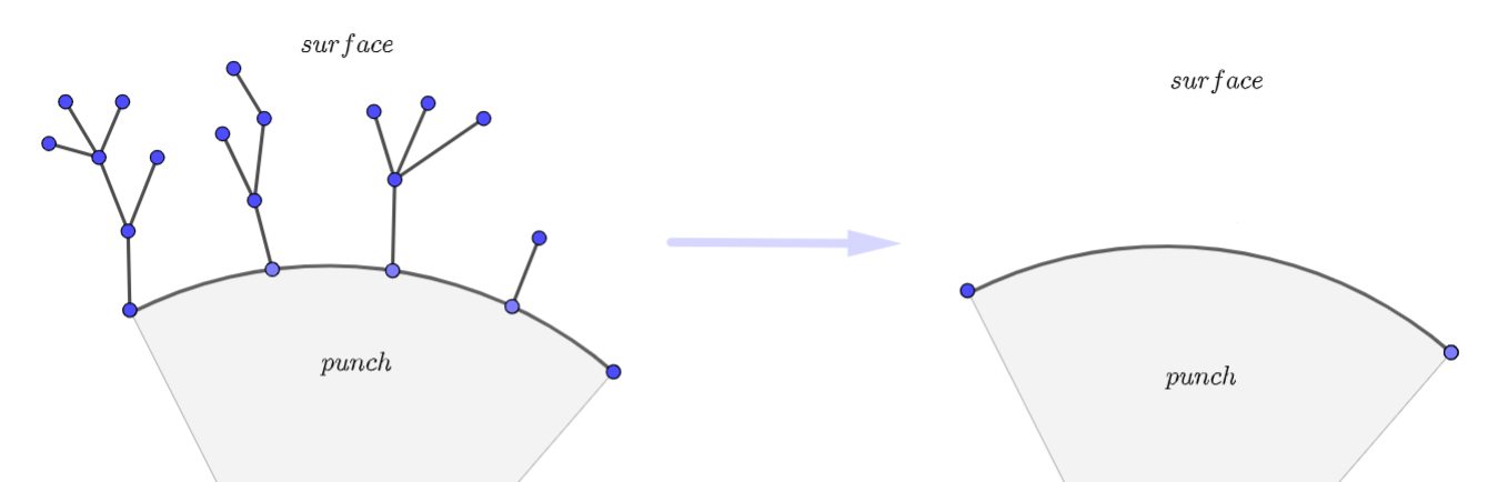
Figure 2: Reduction of a boundary edge

It is worth noting that Okounkov’s contraction does not change the topology of the ribbon graph.

We now state graph expansion for deformed Gaussian IRM. To be precise, for any diagram $\Gamma$, introduce the diagram function.

Definition 2.4.

Given given non-negative integers $k_{1},\dots,k_{s}$, set $k=k_{1}+\cdots+k_{s}$. For the deformed symmetric (resp. Hermitian) Gaussian IRM matrix $X$ defined in Definition 1.1 and for any diagram $\Gamma$, the diagram function of $\Gamma$ associated with $X$ is defined as

$$\mathcal{W}_{\Gamma,X}(k_{1},\dots,k_{s}):=\rho_{a}^{-k}\sum_{\Upsilon:\Phi(\Upsilon)=\Gamma}\sum_{\eta:\mathcal{V}(\Upsilon)\to[N]}\prod_{(x,y)\in\mathcal{E}_{int}(\Upsilon)}\sigma_{\eta(x)\eta(y)}^{2}\prod_{(z,w)\in\mathcal{E}_{b}(\Upsilon)}A_{\eta(z)\eta(w)}.$$ (2.2)

Here the summation $\sum_{\Upsilon}$ is over all $\Upsilon$ such that the reduced diagram is $\Gamma$. Namely, we classify all ribbon graphs according to Okounkov’s contraction.

Proposition 2.5.

Let $X$ be the real symmetric deformed Gaussian IRM matrix defined in (1.9), for any given non-negative integers $k_{1},\dots,k_{s}$. Denoting $k=k_{1}+\cdots+k_{s}$, we have

$$\rho_{a}^{-k}\mathbb{E}[\prod_{j=1}^{s}\mathrm{Tr}X^{k_{j}}]=\sum_{s-{\rm cells\ diagrams\ }\Gamma}\mathcal{W}_{\Gamma,X}(k_{1},\dots,k_{s}).$$ (2.3)

Proof.

Introduce a permutation $\gamma=(12\cdots k_{1})(k_{1}+1\cdots k_{1}+k_{2})\cdots(k_{1}+\cdots+k_{s-1}+1\cdots k)\in\mathcal{S}_{k}$. Let $\eta:[k]\to[N]$ be the map of the labeling. A simple matrix calculation shows

$$\mathbb{E}\Big{[}\prod_{j=1}^{s}\mathrm{Tr}X^{k_{j}}\Big{]} =\sum_{\eta:[k]\to[N]}\mathbb{E}\Big{[}\prod_{j=1}^{k}\big{(}H_{\eta(j)\eta(\gamma(j))}+A_{\eta(j)\eta(\gamma(j))}\big{)}\Big{]}$$

$$=\sum_{\eta:[k]\to[N]}\sum_{\text{J}\subset[k]}\mathbb{E}\Big{[}\prod_{j\in{\rm J}}H_{\eta(j)\eta(\gamma(j))}\Big{]}\prod_{j\in{\rm J^{c}}}A_{\eta(j)\eta(\gamma(j))}.$$ (2.4)

where $\mathcal{P}_{2}(J)$ denote all pairings of $J$. Noting the symmetry of $H$, by the Wick formula we see

$$\mathbb{E}\big{[}\prod_{j\in{\rm J}}H_{\eta(j)\eta(\gamma(j))}\big{]} =\sum_{\pi\in\mathcal{P}_{2}(\text{J})}\prod_{(s,t)\in\pi}\mathbb{E}\big{[}H_{\eta(s)\eta(\gamma(s))}H_{\eta(t)\eta(\gamma(t))}\big{]}$$

$$=\sum_{\pi\in\mathcal{P}_{2}(\text{J})}\prod_{(s,t)\in\pi}\sigma_{\eta(s)\eta(\gamma(s))}^{2}\Big{(}\delta_{\eta(s)\eta(\gamma(t))}\delta_{\eta(t)\eta(\gamma(s))}+\delta_{\eta(\gamma(t))\eta(\gamma(s))}\delta_{\eta(s)\eta(t)}\Big{)}.$$ (2.5)

If $|J|$ is odd, then $\mathbb{E}\big{[}\prod_{j\in{\rm J}}H_{\eta(j)\eta(\gamma(j))}\big{]}=0$. Hence we have

$$\mathbb{E}[\prod_{j=1}^{s}\mathrm{Tr}X^{k_{j}}]=\sum_{\text{J}\subset[k]}\sum_{\pi\in\mathcal{P}_{2}(\text{J})}\sum_{\eta:[k]\to[N]}\prod_{j\in{\rm J^{c}}}A_{\eta(j)\eta(\gamma(j))}\prod_{(s,t)\in\pi}\sigma_{\eta(s)\eta(\gamma(s))}^{2}\Big{(}\delta_{\eta(s)\eta(\gamma(t))}\delta_{\eta(t)\eta(\gamma(s))}+\delta_{\eta(\gamma(t))\eta(\gamma(s))}\delta_{\eta(s)\eta(t)}\Big{)}.$$ (2.6)

The above summation is exactly the enumeration for ribbon graph $\Upsilon$ with subset $J$ and pairing $\pi$.

To be precise, we have

$$\rho_{a}^{-k}\mathbb{E}[\prod_{j=1}^{s}\mathrm{Tr}X^{k_{j}}]=\sum_{\Upsilon}\rho_{a}^{-k}\sum_{\eta:\mathcal{V}(\Upsilon)\to[N]}\prod_{(x,y)\in\mathcal{E}_{int}(\Upsilon)}\sigma_{\eta(x)\eta(y)}^{2}\prod_{(z,w)\in\mathcal{E}_{b}(\Upsilon)}A_{\eta(z)\eta(w)}.$$ (2.7)

Classifying $\Upsilon$ by the contraction map $\Phi(\Upsilon)$ and recall the definition of $\mathcal{W}_{\Gamma,X}(k_{1},\dots,k_{s})$, we thus arrive at

$$\rho_{a}^{-k}\mathbb{E}[\prod_{j=1}^{s}\mathrm{Tr}X^{k_{j}}]=\sum_{{\rm diagrams\ }\Gamma}\mathcal{W}_{\Gamma}(k_{1},\dots,k_{s}).$$ (2.8)

∎

We now simplify the diagram function $\mathcal{W}_{\Gamma}(k_{1},\dots,k_{s})$ in Definition 2.4.

Proposition 2.6.

Let $p_{n}(x,y)$ be the $n$-th step transition probability associated with the Markov matrix $P_{N}$ in Definition 1.1, then for any diagram $\Gamma$ we have

$$\mathcal{W}_{\Gamma,X}(k_{1},\dots,k_{s})=\rho_{a}^{-k}\sum_{\eta:V(\Gamma)\to[N]}\sum_{n_{e}\geq 1,{e\in E(\Gamma)}}\prod_{j=1}^{s}\binom{k_{j}}{\frac{k_{j}-\sum_{\partial D_{j}}n_{e}}{2}}\\ \times\prod_{(x,y)\in E_{int}}p_{n_{e}}(\eta(x),\eta(y))\prod_{(z,w)\in E_{b}}A_{\eta(z)\eta(w)}^{n_{e}}.$$ (2.9)

Proof.

We need to count the pre-images of $\Gamma$ under the Okounkov’s contraction. For any edge $e\in E(\Gamma)$, suppose there are exactly $n_{e}-1$ divalent vertices deleted in the reduction, i.e., there are exactly $n_{e}$ segments before the reduction. So the total number of divalent vertices deleted in $\partial D_{j}$ is $n_{j}:=\sum_{e\in\partial D_{j}}n_{e}$. We then have the total number of all possible trees on the $j$-th face is

$$\sum_{u_{1}+\cdots+u_{n_{j}}=(k_{j}-n_{j})/2,\ u_{i}\geq 0}(2u_{1}+1)\prod_{i=1}^{n_{j}}C_{u_{i}}=\binom{k_{j}}{\frac{k_{j}-n_{j}}{2}},$$ (2.10)

where $C_{n}:=(2n)!/(n!(n+1)!)$ is the $n$-th Catalan number.

Now for $e\in E_{b}$, suppose that we have deleted $n_{e}-1$ divalent vertices in the reduction. Fix $\eta$’s value at the endpoint and sum over all possible vertices, we thus obtain the factor of $A_{\eta(z)\eta(w)}^{n_{e}}$.

Similarly, as for $e\in E_{int}$, fix $\eta$’s value at the endpoint $(\eta(x),\eta(y))$ and sum over all possible values on divalent vertices, by the doubly-stochastic property of $P_{N}$, we obtain the factor of $p_{n_{e}}(\eta(x),\eta(y))$.

Therefore, this completes the proof of the desired result. ∎

Example 2.7 (Degenerate diagram).

After the Okounkov’s reduction, it is possible that the reduced ribbon graph does not contain any vertex with degree at least 3. Such diagram is said to be a degenerate diagram. In the deformed IRM model, the only degenerate diagram $\Gamma_{0}$ is a circle with a marked point and hence only appears in the special case $s=1$, as shown in the figure below. The weight of this diagram can be calculated as follows

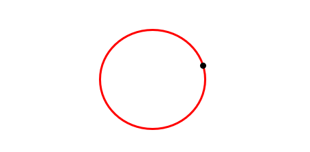
Figure 3: degenerate diagram

$$\mathcal{W}_{\Gamma_{0},X}(k) =\rho_{a}^{-k}\sum_{n\geq 1}\sum_{d_{1}+\dots+d_{n}=\frac{k-n}{2}}(2d_{1}+1)C_{d_{1}}\cdots C_{d_{n}}\mathrm{Tr}A_{N}^{n}$$

$$=\rho_{a}^{-k}\sum_{n\geq 1}\binom{k}{\frac{k-n}{2}}\mathrm{Tr}A_{N}^{n}.$$ (2.11)

The circle corresponds to the law of large numbers of the largest outlier eigenvalue.

In order to give upper bounds for diagram functions, it’s convenient for later use to introduce a new quantity by taking absolute value in the last factor

$$\mathcal{W}^{+}_{\Gamma,X}(k_{1},\dots,k_{s})=\rho_{a}^{-k}\sum_{\eta:V(\Gamma)\to[N]}\sum_{n_{e}\geq 1,{e\in E(\Gamma)}}\prod_{j=1}^{s}\binom{k_{j}}{\frac{k_{j}-\sum_{\partial D_{j}}n_{e}}{2}}\\ \times\prod_{(x,y)\in E_{int}}p_{n_{e}}(\eta(x),\eta(y))\prod_{(z,w)\in E_{b}}|A_{\eta(z)\eta(w)}^{n_{e}}|.$$ (2.12)

Remark 2.1 (Variations of ribbon graph expansion).

In this remark, we state two variations of ribbon graph expansion, which are both useful for further discussions.

• In the above discussions, unconnected ribbon graphs and diagrams are included. In fact, one can just focus on the connected ones via the well-known transforms:

  $$\begin{gathered}T(k_{1})=\rho_{a}^{-k_{1}}\mathbb{E}[\mathrm{Tr}X^{k_{1}}],\\ T\big{(}k_{1},k_{2}\big{)}=\rho_{a}^{-k_{1}-k_{2}}\mathbb{E}[\mathrm{Tr}X^{k_{1}}\mathrm{Tr}X^{k_{2}}]-T\big{(}k_{1}\big{)}T\big{(}k_{2}\big{)},\\ \cdots\\ T\big{(}k_{1},\cdots,k_{s}\big{)}=\rho_{a}^{-k_{1}-k_{2}\cdots-k_{s}}\mathbb{E}[\mathrm{Tr}X^{k_{1}}\mathrm{Tr}X^{k_{2}}\ldots\mathrm{Tr}X^{k_{s}}]-\sum_{\Pi}\prod_{P\in\Pi}T\big{(}\{k_{j}\}_{j\in P}\big{)},\end{gathered}$$ (2.13)

  where the summation is over all nontrivial partitions $\Pi$ of $\{1,2,\cdots,s\}$ into disjoint sets. The inversion formulas read

  $$\rho_{a}^{-k_{1}-k_{2}-\cdots-k_{s}}\mathbb{E}[\prod_{j=1}^{s}\mathrm{Tr}X^{k_{j}}]=\sum_{\Pi}\prod_{P\in\Pi}T(\{n(j)\}_{j\in P}),$$ (2.14)

  where the summation is over all all partitions $\Pi$ of $[s]$.

  In fact one can check that $T\big{(}k_{1},\cdots,k_{s}\big{)}$ is related to the enumeration of connected diagrams. Namely,

  $$T\big{(}k_{1},\cdots,k_{s}\big{)}=\sum_{{\rm connected\ diagrams\ }\Gamma}\mathcal{W}_{\Gamma}(k_{1},\dots,k_{s})$$ (2.15)

  Connected diagrams are easier to handle. One possible reason is that each compact connected topological surface is uniquely determined by the following 3 invariants: the genus $g$, the number of “punctures” $t$ and orientable or not. In Section 3, we mainly focus on connected ribbon graphs and give an upper bound for the diagram function.

• Essentially, we only need to consider these diagrams $\Gamma$ such that $E_{b,j}(\Gamma)\neq\emptyset$. To be precise, one has the following variation of ribbon graph expansion.

  $$\rho_{a}^{-k}\mathbb{E}[\prod_{j=1}^{s}(\mathrm{Tr}X^{k_{j}}-\mathrm{Tr}H^{k_{j}})]=\sum_{\Gamma:E_{b},j(\Gamma)\neq\emptyset\text{ for each }j}\mathcal{W}_{\Gamma}(k_{1},\dots,k_{s}).$$ (2.16)

  And in Section 5, we will show that under the conditions in Theorem 1.3, one has

  $$\rho_{a}^{-k}\mathbb{E}[\prod_{j=1}^{s}\mathrm{Tr}X^{k_{j}}]\sim\rho_{a}^{-k}\mathbb{E}[\prod_{j=1}^{s}(\mathrm{Tr}X^{k_{j}}-\mathrm{Tr}H^{k_{j}})],$$ (2.17)

  which helps us rule out other diagrams.

2.2 Graph expansions for non-Gaussian IRM

In the non-Gaussian setting one cannot directly use the Wick formula, so we need new techniques to develop ribbon graph expansions. A natural argument is to compare the moments with those in the Gaussian case. This gives a similar expansion taking in a similar form but admitting complicated coupling factors.

For ribbon graph $\Upsilon$, with the same notations in Definition 1.1, introduce new notations as follows.

1. Let $W_{N}=(W_{xy})$ be a Wigner matrix, for $1\leq x\neq y\leq N$ and $n_{1},n_{2}\geq 1$ with $n_{1}+n_{2}$ even, define

   $$c_{xy}(n_{1},n_{2})=\frac{\mathbb{E}[W_{xy}^{n_{1}}W_{yx}^{n_{2}}]}{\mathbb{E}[|\mathcal{N}(0,1)|^{n_{1}+n_{2}}]},$$ (2.18)

   while for $1\leq x\leq N$ and even number $n\geq 1$,

   $$c_{x}(n)=\frac{\mathbb{E}[W_{xx}^{n}]}{\mathbb{E}[|\mathcal{N}(0,2)|^{n}]}.$$ (2.19)

2. For $\eta:\mathcal{V}(\Upsilon)\to[N]$, $n_{\vec{xy}}(\eta)$ denotes the order of moments of $H_{xy}$ in the product $\prod_{j\in{\rm J}}H_{\eta(j),\eta(\gamma(j))}$, that is, $n_{\vec{xy}}(\eta)$ is the number of directed interior edges in $\Upsilon$ such that the evaluation of $\eta$ on starting and ending points are exactly $x$ and $y$. In particular, set $n_{x}(\eta):=n_{\vec{xx}}(\eta)$.

3. The coupling factor

   $$c(\Upsilon,\eta):=\prod_{1\leq x<y\leq N}c_{xy}(n_{\vec{xy}}(\eta),n_{\vec{yx}}(\eta))\prod_{1\leq x\leq N}c_{x}(n_{x}(\eta)),$$ (2.20)

   is used to measure the difference between the sub-Gaussian $H$ and Gaussian IRM ensembles with the same variance profile.

4. For the sub-Gaussian matrix $X$ defined in Definition 1.1 and any diagram $\Gamma$, define the diagram function

   $$\mathcal{W}_{\Gamma,X}(k_{1},\dots,k_{s}):=\rho_{a}^{-k}\sum_{\Upsilon:\Phi(\Upsilon)=\Gamma}\sum_{\eta:\mathcal{V}(\Upsilon)\to[N]}c(\Upsilon,\eta)\prod_{(x,y)\in\mathcal{E}_{int}(\Upsilon)}\sigma_{\eta(x)\eta(y)}^{2}\prod_{(z,w)\in\mathcal{E}_{b}(\Upsilon)}A_{\eta(z)\eta(w)}.$$ (2.21)

   In particular, if $X$ is a deformed real Gaussian IRM studied in Section 2.1, then $c(\Upsilon,\eta)=1$, hence the definition here coincides with Definition 2.4.

Proposition 2.8.

Let $X=X_{N}$ be the symmetric/Hermitian IRM matrix in Definition 1.1, with $\mathcal{W}_{\Gamma,X}$ in (2.21) we have

$$\rho_{a}^{-k}\mathbb{E}[\prod_{j=1}^{s}\mathrm{Tr}X^{k_{j}}]=\sum_{s-{\rm cells\ diagrams\ }\Gamma}\mathcal{W}_{\Gamma,X}(k_{1},\dots,k_{s}).$$ (2.22)

Proof of Proposition 2.8.

Let $\gamma=(12\cdots k_{1})(k_{1}+1\cdots k_{1}+k_{2})\cdots(k_{1}+\cdots+k_{s-1}\cdots k)\in\mathcal{S}_{k}$. A simple matrix calculation shows

$$\mathbb{E}\Big{[}\prod_{j=1}^{s}\mathrm{Tr}X^{k_{j}}\Big{]} =\sum_{\eta:[k]\to[N]}\mathbb{E}\Big{[}\prod_{j=1}^{k}\big{(}H_{\eta(j),\eta(\gamma(j))}+A_{\eta(j),\eta(\gamma(j))}\big{)}\Big{]}$$ (2.23)

$$=\sum_{\eta:[k]\to[N]}\sum_{\text{J}\subset[k]}\mathbb{E}\Big{[}\prod_{j\in{\rm J}}H_{\eta(j),\eta(\gamma(j))}\Big{]}\prod_{j\in{\rm J^{c}}}A_{\eta(j),\eta(\gamma(j))}.$$

By the definition of $c(\Upsilon,\eta)$, we have

$$\mathbb{E}\big{[}\prod_{j\in{\rm J}}H_{\eta(j),\eta(\gamma(j))}\big{]}=c(\Upsilon,\eta)\mathbb{E}\big{[}\prod_{j\in{\rm J}}H^{\rm Gaussian}_{\eta(j),\eta(\gamma(j))}\big{]}$$ (2.24)

$$=c(\Upsilon,\eta)\sum_{\pi\in\mathcal{P}_{2}(\text{J})}\prod_{(s,t)\in\pi}\mathbb{E}\big{[}H_{\eta(s),\eta(\gamma(s))}H_{\eta(t),\eta(\gamma(t))}\big{]}$$

$$=c(\Upsilon,\eta)\sum_{\pi\in\mathcal{P}_{2}(\text{J})}\prod_{(s,t)\in\pi}\sigma_{\eta(s),\eta(\gamma(s))}^{2}\big{(}\delta_{\eta(s),\eta(\gamma(t))}\delta_{\eta(t),\eta(\gamma(s))}+\delta_{\eta(s),\eta(t)}\delta_{\eta(\gamma(t)),\eta(\gamma(s))}\big{)}.$$

Note that if $|J|$ is odd, we have $\mathbb{E}\left[\prod_{j\in{\rm J}}H_{\eta(j),\eta(\gamma(j))}\right]=0$.

Similar to the argument in Proposition 2.5, Glue the polygons $D_{1},\dots,D_{s}$ to ribbon graphs and note that the term $c(\Upsilon,\eta)$ has no effect on gluing polygons, we can use ribbon graph enumeration to rewrite

$$\mathbb{E}[\prod_{j=1}^{s}\mathrm{Tr}X^{k_{j}}]=\sum_{S}\sum_{\Upsilon}\sum_{\eta:\mathcal{V}(\Upsilon)\to[N]}c(\Upsilon,\eta)\prod_{(x,y)\in\mathcal{E}_{int}(\Upsilon)}\sigma_{\eta(x)\eta(y)}^{2}\prod_{(z,w)\in\mathcal{E}_{b}(\Upsilon)}A_{\eta(z)\eta(w)}.$$ (2.25)

Substituting of (2.21) into the above completes the proof of Proposition 2.8. ∎

We remark that the coupling factor in Proposition 2.8 is different in the real and complex cases. In the real case, the second moment part is always 1, but in the complex case, the second moment of diagonal entries $c_{x}(2)=\frac{1}{2}$ and $c_{xy}(2,0)=0$, $c_{xy}(1,1)=1$ for $x\neq y$. Besides, the term $c(\Upsilon,\eta)$ is too complicated to admit explicit expressions in the non-Gaussian case, compared to Proposition 2.6. We will return to have a more thorough treatment in Section 3.2 and Section 5.

2.3 Trivalent and typical diagrams

For further discussions, the following notations will be in force from now on and may be used frequently in the whole paper.

Notations:

1. Denote $\Gamma_{g,t,s}^{\geq 3}$ be the set of connected diagrams with $t$ punctures and $s$ cells such that its Euler characteristic $\chi(\Gamma)=2-g-t$.

2. Denote $\Gamma_{g,t,s}^{=3}$ the subset of trivalent diagrams in $\Gamma_{g,t,s}^{\geq 3}$.

3. Denote $\Gamma_{g,t,s}^{\geq 3,b}$ the subset of $\Gamma_{g,t,s}^{\geq 3}$ such that the number of boundary edges on the $j-$th face is at least one. Namely, $E_{b,j}\neq\emptyset$ for each $j\in[s]$.

4. Set $\Gamma_{g,t,s}^{=3,b}:=\Gamma_{g,t,s}^{=3}\cap\Gamma_{g,t,s}^{\geq 3,b}$ the set of trivalent diagrams in $\Gamma_{g,t,s}^{\geq 3}$.

The following graph inequality is of central importance in counting dominant diagrams, which connects boundary edges, interior vertices and faces.

Lemma 2.9.

For any diagram $\Gamma$ with $s$-cells, we have

$$|E_{b}(\Gamma)|+3|V_{int}(\Gamma)|\leq 2|E_{int}(\Gamma)|+s.$$ (2.26)

Moreover, the equality holds if and only if $\Gamma$ is trivalent and the marked points are distinct.

Proof.

Recall that each unmarked vertex in $\Gamma$ has degree greater than or equal to 3, each marked point has degree at least 2 and any loop incident to the vertex is counted twice, we obtain

$$2|E_{b}(\Gamma)|+2|E_{int}(\Gamma)|=\sum_{v\in V(\Gamma)}{\rm deg}_{\Gamma}(v)\geq 3|V(\Gamma)|-s=3|V_{b}(\Gamma)|+3|V_{int}(\Gamma)|-s.$$ (2.27)

We claim that the boundary of $\Gamma$, which is a subgraph of $\Gamma$ generated by the boundary edges, is just a disjoint union of some circles. This can be easily proved from either the topological viewpoint or the graph theoretical viewpoint.

Topologically, the boundary of $\Gamma$, as the boundary of a 2-dimensional compact manifold, is a 1-dimensional closed manifold, hence is a disjoint union of some circles.

In terms of graph theory, by construction of the gluing operation, one can show that for each boundary vertex, its degree in the boundary subgraph is exactly 2. In fact, firstly, one can check the degree of each boundary vertex in the boundary subgraph is even, because the total degree of this vertex is even, and each interior arc on the polygon is paired with another one; secondly, in each step of the gluing, the degree of each boundary vertex in the boundary subgraph is at most two. Besides, again the vertex degree of a self-loop is 2.

Since $n$ boundary vertices on a circle divide the circle into $n$ arcs, i.e. $n$ boundary edges, the above claim gives us an equality

$$|E_{b}(\Gamma)|=|V_{b}(\Gamma)|.$$ (2.28)

Together with (2.27), we get the inequality (2.26). Moreover, the equality holds if and only if that in (2.27) holds, further if and only if $\Gamma$ is trivalent, and marked points of $\Gamma$ are distinct. ∎

Lemma 2.10.

For trivalent diagram $\Gamma\in\Gamma_{g,t,s}^{=3,b}$, then we have

$$|V(\Gamma)|=2g+2t+3s-4,\quad|E(\Gamma)|=3g+3t+4s-6.$$ (2.29)

Set $l=|V_{int}({\Gamma})|$, we have

$$|V_{b}({\Gamma})|=|E_{b}({\Gamma})|=2g+2t+3s-4-l,\quad|E_{int}({\Gamma})|=g+t+s+l-2.$$ (2.30)

Proof.

Since each unmarked points in $V(\Gamma)$ is trivalent, and each marked points are distinct and divalent. We see that

$$2|E(\Gamma)|=\sum_{v\in V(\Gamma)}{\rm deg}_{\Gamma}(v)=3(|V(\Gamma)|-s)+2s=3|V(\Gamma)|-s.$$ (2.31)

Now we use the Euler formula for the ribbon graph $\Gamma$ (in fact, for the background surface of $\Gamma$) to see

$$|V(\Gamma)|-|E(\Gamma)|+s=\chi(\Gamma)=2-g-t.$$ (2.32)

So (2.29) directly follows from (2.31) and (2.32), and (2.30) directly follows from (2.29) and (2.28). ∎

To characterize the fluctuation we introduce a family of special typical ribbon graphs that are dominant at the level of outlier fluctuation.

Definition 2.11.

A diagram $\Gamma$ is called typical , if it is a trivalent graph such that $V_{int}(\Gamma)=\emptyset$ and each marked point is a boundary vertex. Equivalently, $\Gamma$ is typical if and only if $|E_{b}(\Gamma)|=2|E_{int}(\Gamma)|+s$. Otherwise, it is called a non-typical diagram. Several typical and non-typical diagrams are listed in Figure 4.

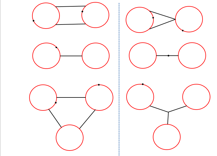
Figure 4: typical (left) VS non-typical diagrams (right) where boundary edges are colored red.

By Lemma 2.9 we see that typical diagrams have the most boundary edges among all diagrams in $\Gamma_{g,t,s}^{\geq 3}$. This property implies tha all typical diagrams have the largest freedom in counting. Besides, there is a natural correspondence between typical diagrams and ordinary ribbon graphs on the closed surface: If we shrink each hole in a typical diagram to a point, we get a ribbon graph on the closed surface. Conversely, every typical diagram can be recovered by enlarging vertices of a ribbon graph to a hole.

3 Upper bound estimates

Our goal in this section is to obtain term-wise upper bounds for diagram functions. These can be treated as dominating functions in Domination Convergence Theorem. The basic philosophy behind is that GOE (with a smaller size such that the sparsity are matched) can dominate sub-Gaussian IRM matrix. For this purpose, throughout this section, we frequently use the following rank-1 deformation of the normalized GOE, denoted by $Y_{M}$.

$$Y_{M}=H_{{\rm GOE}_{M}}+aE_{11}=\frac{1}{\sqrt{M}}W_{{\rm GOE}_{M}}+aE_{11}.$$ (3.1)

Now we introduce the dominating function and state main results in this section.

Definition 3.1.

Given parameters $s\geq 1$ and $\lambda,a>1$, the dominating function of variables $g\geq 0$ and $t\geq 1$ is defined as

$$\mathcal{D}_{g,t,s}(\xi;a,\lambda):=(2\xi s)^{2g+2t+2s-4}\Big{(}\frac{2\lambda a^{2}}{a^{2}-1}\Big{)}^{3g+3t+4s-6}\frac{2048^{g+t+2s}}{(g+t)!}.$$ (3.2)

Theorem 3.2.

With $X_{N}$ given in Definition 1.1 and with $\mathcal{W}_{\Gamma}$ in (2.21), assume that

$$\sum_{j=1}^{s}k_{j}\leq\frac{\xi}{\sqrt{\gamma}(r+1)\sigma_{N}^{*}}$$ (3.3)

for any fixed $\xi>0$, then for any integer $g\geq 0$ and $t\geq 1$ we have

$$\sum_{\Gamma\in\Gamma_{g,t,s}^{\geq 3,b}}|\mathcal{W}_{\Gamma,X_{N}}(k_{1},\cdots,k_{s})|\leq r^{s}e^{4\xi^{2}}\mathcal{D}_{g,t,s}(\xi;a,1).$$ (3.4)

Furthermore, there exist positive constants $C_{1}(s,a)$ and $C_{2}(s,a)$ depending on $s,a$ such that

$$\sum_{g\geq 0}\sum_{t\geq 1}\mathcal{D}_{g,t,s}(\xi;a,1)\leq C_{1}(s,a)\exp\!\left\{C_{2}(s,a)\xi^{2}\right\}.$$ (3.5)

We will first prove a GOE special case of Theorem 3.2, since the GOE dominates sub-Gaussian IRM.

Theorem 3.3.

Let $Y_{M}$ be given in (3.1), if $k=\sum_{j=1}^{s}k_{j}\leq\xi\sqrt{M}$, then

$$\sum_{\Gamma\in\Gamma_{g,t,s}^{\geq 3,b}}\lambda^{|E(\Gamma)|}\mathcal{W}_{\Gamma,Y_{M}}(k_{1},\cdots,k_{s})\leq\mathcal{D}_{g,t,s}(\xi;a,\lambda),$$ (3.6)

and

$$\sum_{g\geq 0}\sum_{t\geq 1}\mathcal{D}_{g,t,s}(\xi;a,\lambda)\leq C_{1}(s,a,\lambda)\exp\left\{C_{2}(s,a,\lambda)\xi^{2}\right\}$$ (3.7)

for some constants $C_{1}(s,a,\lambda),C_{2}(s,a,\lambda)>0.$

Theorem 3.4.

With $X_{N}$ given in Definition 1.1 and $\mathcal{W}_{\Gamma,X_{N}}$ in (2.21), assume that the integer $M>0$ satisfies $M\gamma((r+1)\sigma_{N}^{*})^{2}\leq 1$ and $k:=k_{1}+\cdots+k_{s}\leq\frac{1}{2}M$. For any connected ribbon graph $\Gamma\in\Gamma_{g,t,s}^{\geq 3}$, if $\Gamma$ contains any boundary edge, then

$$\left|\mathcal{W}_{\Gamma,X_{N}}(k_{1},\dots,k_{s})\right|\leq r^{s}e^{\frac{3k^{2}}{M}+\frac{k}{M}}\mathcal{W}_{\Gamma,Y_{M}}(k_{1},\dots,k_{s}),$$ (3.8)

while if $\Gamma$ contains no boundary edge,

$$\left|\mathcal{W}_{\Gamma,X_{N}}(k_{1},\dots,k_{s})\right|\leq NM^{-1}e^{\frac{3k^{2}}{M}}\mathcal{W}_{\Gamma,Y_{M}}(k_{1},\dots,k_{s})$$ (3.9)

Theorem 3.2 immediately follows from Theorem 3.3 and Theorem3.4.

Proof of Theorem 3.2.

We only need to consider the diagram $\Gamma\in\Gamma_{g,t,s}^{\geq 3,b}$. By Theorem 3.4, we have

$$\left|\mathcal{W}_{\Gamma,X_{N}}(k_{1},\dots,k_{s})\right|\leq r^{s}e^{\frac{4k^{2}}{M}}\mathcal{W}_{\Gamma,Y_{M}}(k_{1},\dots,k_{s}).$$ (3.10)

Here we need to take $M\gamma((r+1)\sigma_{N}^{*})^{2}\leq 1$ and $k\leq{M}/{2}$. We also use the simple inequality ${k}/{M}\leq{k^{2}}/{M}$. Theorem 3.3 immediately implies the first inequality of Theorem 3.3.

The second inequality of Theorem 3.3 is the same as that of Theorem 3.3. ∎

It is worth stressing that Theorem 3.2 affords a dominating function for the diagram functions with parameter $g,t$. By DCT, to study asymptotic behavior for the sum of all diagrams, it suffices to consider asymptotics for the sum of diagrams with parameter $g,t$. Since there are only finite diagram functions with such parameters, we only need to consider the limit of diagram function diagram-wisely.

3.1 Dominating functions for GOE

In this subsection, we prove Theorem 3.3, which gives us a natural dominating function for all diagrams. Recall that $Y_{M}$ is the $M\times M$ deformed matrix model defined in (3.1).

Roughly speaking, our proof is divided into three parts: Firstly, we give a diagram-wise upper bound of the weight function $\mathcal{W}_{\Gamma,Y_{M}}(k_{1},\cdots,k_{s})$. Secondly, we regularize all diagrams to trivalent diagrams. Thirdly, we bound the number of trivalent diagrams via automation created in [FS10]. The proof of Theorem 3.3 directly follows from these three steps.

Proof of Theorem 3.3: Step 1. We first give an upper bound for $\mathcal{W}_{\Gamma,Y_{M}}(k_{1},\cdots,k_{s})$.

Proposition 3.5.

For any diagram $\Gamma\in\Gamma_{g,t,s}^{\geq 3,b}$ and for any positive integer $k_{1},\dots,k_{s}$, we have

$$\mathcal{W}_{\Gamma,Y_{M}}(k_{1},\cdots,k_{s})\leq\big{(}\frac{a^{2}}{a^{2}-1}\big{)}^{|E(\Gamma)|}\Big{(}\frac{1}{M}\Big{)}^{|E_{int}|-|V_{int}|}\prod_{j=1}^{s}\frac{k_{j}^{|E_{b,j}|-1}}{(|E_{b_{j}}|-1)!}:=\widetilde{\mathcal{W}}_{\Gamma,Y_{M}}(k_{1},\cdots,k_{s}).$$ (3.11)

Proof of Proposition 3.5.

By the definition of $\mathcal{W}_{\Gamma,Y_{M}}(k_{1},\dots,k_{s})$, noting that $k=k_{1}+\cdots+k_{s}$, one gets

$$\mathcal{W}_{\Gamma,Y_{M}}(k_{1},\dots,k_{s}) =\rho_{a}^{-k}\sum_{\eta:V(\Gamma)\to[M]:\eta|_{V_{b}}=1}\sum_{n_{e}\geq 1}\prod_{j=1}^{s}\binom{k_{j}}{\frac{1}{2}\big{(}k_{j}-\sum_{\partial D_{j}}n_{e}\big{)}}\prod_{(x,y)\in E_{int}}M^{-1}\prod_{(z,w)\in E_{b}}a^{n_{e}}$$ (3.12)

$$= \rho_{a}^{-k}\sum_{\eta:V(\Gamma)\to[M]:\eta|_{V_{b}}=1}\sum_{n_{e}\geq 1}a^{\sum_{e\in E_{b}}n_{e}}\prod_{j=1}^{s}\binom{k_{j}}{\frac{1}{2}\big{(}k_{j}-\sum_{\partial D_{j}}n_{e}\big{)}}\prod_{(x,y)\in E_{int}}M^{-1}$$

$$\leq \sum_{n_{e}\geq 1}\big{(}\frac{1}{M}\big{)}^{|E_{int}|-|V_{int}|}\prod_{j=1}^{s}\binom{k_{j}}{\frac{1}{2}\big{(}k_{j}-\sum_{\partial D_{j}}n_{e}\big{)}}\rho_{a}^{-k_{j}}a^{\sum_{e\in E_{b}}n_{e}}.$$

To bound the summation over $n_{e}$, we consider boundary edges and inner edges separately. Recall that $E_{b,j}$ is the set of boundary edges in $\partial D_{j}$. Let $n_{j}=\sum_{e\in\partial D_{j}}n_{e}$ be the total length of segments of $\partial D_{j}$ after reduction, $n_{j}^{\rm b}=\sum_{e\in E_{b,j}}n_{e}$ be the total length of boundary edges in $\partial D_{j}$ and $n_{j}^{\rm int}=\sum_{e\in\partial D_{j}\cap E_{int}}n_{e}$(counting twice if some interior edge $e$ appears twice in $D_{j}$) be the total length of interior segments of $\partial D_{j}$.

Fixing $(n_{j})_{j\in[s]}$, there are at almost

$$\binom{n^{b}_{j}}{|E_{b,j}|-1}\leq\frac{{n_{j}}^{|E_{b,j}|-1}}{(|E_{b,j}|-1)!}$$

solutions for a system of equations

$$\mathfrak{C}_{j}:\sum_{e\in E_{b,j}}n_{e}=n^{b}_{j},\quad j=1,2,\dots,s.$$ (3.13)

Hence we have

$$\sum_{n_{e}\geq 1}\prod_{j=1}^{s}\binom{k_{j}}{\frac{1}{2}\big{(}k_{j}-\sum_{\partial D_{j}}n_{e}\big{)}}\rho_{a}^{-k_{j}}a^{\sum_{e\in E_{b}}n_{e}}\leq\sum_{n_{e}\geq 1,e\in E_{int}}\sum_{n_{j}^{b}\geq 1}\prod_{j=1}^{s}\binom{k_{j}}{\frac{k_{j}-n_{j}}{2}}\frac{{n_{j}}^{|E_{b,j}|-1}}{(|E_{b,j}|-1)!}\rho_{a}^{-k_{j}}a^{n^{b}_{j}}$$ (3.14)

$$\leq\sum_{n_{e}\geq 1,e\in E_{int}}\sum_{n_{j}\geq 1}\prod_{j=1}^{s}\binom{k_{j}}{\frac{k_{j}-n_{j}}{2}}\frac{{n_{j}}^{|E_{b,j}|-1}}{(|E_{b,j}|-1)!}\rho_{a}^{-k_{j}}a^{n_{j}}\prod_{e\in E_{int}}a^{-2n_{e}}.$$

For the inner sum, we use the binomial distribution

$$\mathbb{P}\left(\text{Binom}(k,\frac{a^{2}}{a^{2}+1})=\frac{k+n}{2}\right)=\rho_{a}^{-k}a^{n}\binom{k}{\frac{k-n}{2}}.$$ (3.15)

to obtain

$$\rho_{a}^{-k_{j}}\sum_{n_{j}\geq 0}a^{n_{j}}\frac{n_{j}^{|E_{b,j}|-1}}{(|E_{b,j}|-1)!}\binom{k_{j}}{\frac{k_{j}-n_{j}}{2}}\leq\frac{k_{j}^{|E_{b,j}|-1}}{(|E_{b,j}|-1)!}\sum_{n_{j}\geq 0}\frac{a^{n_{j}}}{\rho_{a}^{k_{j}}}\binom{k_{j}}{\frac{k_{j}-n_{j}}{2}}\leq\frac{k_{j}^{|E_{b,j}|-1}}{(|E_{b,j}|-1)!},$$ (3.16)

Hence

$$\sum_{n_{e}\geq 1}\prod_{j=1}^{s}\binom{k_{j}}{\frac{1}{2}\big{(}k_{j}-\sum_{\partial D_{j}}n_{e}\big{)}}\rho_{a}^{-k_{j}}a^{\sum_{e\in E_{b}}n_{e}} \leq\prod_{j=1}^{s}\frac{k_{j}^{|E_{b,j}|-1}}{(|E_{b_{j}}|-1)!}\sum_{n_{e}\geq 0}\prod_{e=(x,y)\in E_{int}}\frac{1}{a^{2n_{e}}}$$ (3.17)

$$=\prod_{j=1}^{s}\frac{k_{j}^{|E_{b,j}|-1}}{(|E_{b_{j}}|-1)!}\Big{(}\frac{a^{2}}{a^{2}-1}\Big{)}^{|E_{int}|}.$$

By $|E_{b}|=|V_{b}|$, (3.12) and (3.17), we thus arrive at

$$\mathcal{W}_{\Gamma,Y_{M}}(k_{1},\cdots,k_{s})\leq \big{(}\frac{a^{2}}{a^{2}-1}\big{)}^{|E(\Gamma)|}\Big{(}\prod_{j=1}^{s}\frac{k_{j}^{|E_{b,j}|-1}}{(|E_{b_{j}}|-1)!}\Big{)}\Big{(}\frac{1}{M}\Big{)}^{|E_{int}|-|V_{int}|}.$$ (3.18)

This completes the proof. ∎

Remark 3.1.

In fact the discussion here is adaptive for a wider class of diagrams. Precisely, consider a diagram $\Gamma$ with $r$ ($\geq s$) distinct marked points, each one is on the boundary. One can also define the weight function by the same equation as in (2.9), and the upper bounds in Proposition 3.5 still holds in this case.

Then, we regularize each diagram $\Gamma\in\Gamma_{g,t,s}^{\geq 3,b}$ to $\bar{\Gamma}\in\Gamma_{g,t,s}^{=3,b}$

Proposition 3.6.

For $\lambda\geq 1$, we have

$$\sum_{\Gamma\in\Gamma_{g,t,s}^{\geq 3,b}}\lambda^{|E(\Gamma)|}\widetilde{\mathcal{W}}_{\Gamma,Y_{M}}(k_{1},\cdots,k_{s})\leq\sum_{\Gamma\in\Gamma_{g,t,s}^{=3,b}}(2\lambda)^{|E(\Gamma)|}\widetilde{\mathcal{W}}_{\Gamma,Y_{M}}(k_{1},\cdots,k_{s}).$$ (3.19)

Proof of Proposition 3.6.

For vertices with degree $>3$ and any marked point with degree $>2$, we add a weight 1 edge to split the vertices to those with smaller degree. Namely, we construct a function regularizing each diagram $\Gamma\in\Gamma_{g,t,s}^{\geq 3}$ to a trivalent diagram $\bar{\Gamma}\in\Gamma_{g,t,s}^{=3}$ as figure 5 shows.

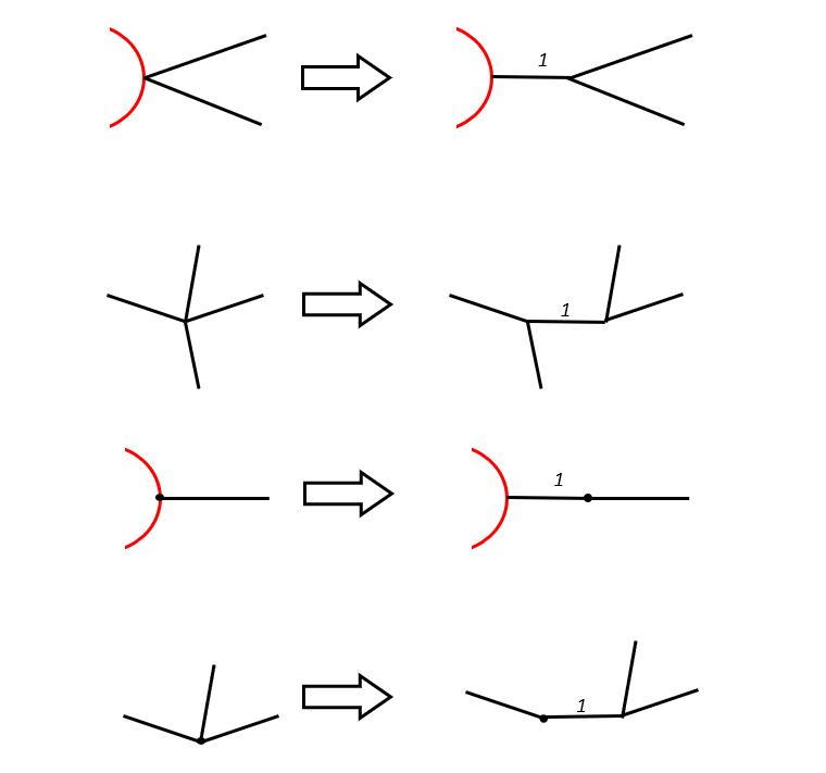
Figure 5: Regularize to trivalent diagrams

Note that the label (viewed as a function $w:E_{int}(\bar{\Gamma})\longrightarrow\{\phi,1\}$) is used to indicate the regularizing process. By using the function $w$, one can rewrite the summation as

$$\sum_{\text{diagrams in }\Gamma_{g,t,s}^{\geq 3}}=\sum_{\bar{\Gamma}\in\Gamma_{g,t,s}^{=3}}\sum_{w}.$$ (3.20)

Note that the qualities $|E_{b,j}|$, $|E_{int}|-|V_{int}|$ do not change after regularization, i.e.

$$|E_{b,j}(\bar{\Gamma})|=|E_{b,j}(\Gamma)|,\quad|E_{int}(\bar{\Gamma})|-|V_{int}(\bar{\Gamma})|=|E_{int}(\Gamma)|-|V_{int}(\Gamma)|,$$ (3.21)

we thus get

$$\widetilde{\mathcal{W}}_{\Gamma,Y_{M}}(k_{1},\cdots,k_{s})\leq\widetilde{\mathcal{W}}_{\bar{\Gamma},Y_{M}}(k_{1},\cdots,k_{s}).$$ (3.22)

Also note that for any regularized diagram $\bar{\Gamma}$, the number of $w:E_{int}(\bar{\Gamma})\longrightarrow\{\phi,1\}$) is at most $2^{|E_{int}(\bar{\Gamma})|}\leq 2^{|E(\bar{\Gamma})|}$, we see from the simple facts $\lambda\geq 1$ and $|E(\bar{\Gamma})|\geq|E(\Gamma)|$ that

$$\sum_{g\geq 0}\sum_{t\geq 0}\sum_{\Gamma\in\Gamma_{g,t,s}^{\geq 3,b}}\lambda^{|E(\Gamma)|}\widetilde{\mathcal{W}}_{\Gamma,Y_{M}}(k_{1},\cdots,k_{s})\leq\sum_{g\geq 0}\sum_{t\geq 0}\sum_{\Gamma\in\Gamma_{g,t,s}^{=3,b}}(2\lambda)^{|E(\Gamma)|}\widetilde{\mathcal{W}}_{\Gamma,Y_{M}}(k_{1},\cdots,k_{s}).$$ (3.23)

This completes the proof. ∎

Proof of Theorem 3.3: Step 2. Next, we will bound the number of trivalent diagrams $|\Gamma_{g,t,s}^{=3}|$.

We follow the argument in [FS10] with slight modifications, where an automation is constructed to generate all possible trivalent $s$-diagrams on closed topological surface. In fact, this automation mechanics can also generate all trivalent diagrams $\Gamma\in\Gamma_{g,t,s}^{=3}$, by additionally demanding that exactly $t$ circles are NOT annihilated in the end. Inspired by the proof of [FS10, Proposition II.3.3] we can obtain an upper bound for $|\Gamma_{g,t,s}^{=3}|$.

Proposition 3.7.

For any $g\geq 0$ and $t,s\geq 1$, we have an upper bound for the number of trivalent diagrams

$$\left|\Gamma_{g,t,s}^{=3}\right|\leq\frac{128^{g+t+2s}(g+t+2s)^{g+t+3s-3}}{(s-1)!}.$$ (3.24)

Proof.

For technical reasons, for each marked point of the diagram, we add an interior edge and reduce the valence of each marked point to 1. Now we use the automation to bound the number of $\Gamma_{g,t,s}^{=3}$.

Note that the number of total steps is $g+t+2s-2$. We first fix the times that our automation starts from these $s$ marked points and back. Suppose the automation starts from the marked point of the first face $D_{1}$ and back to it after $T_{1}$ steps, and then start from marked point of $D_{2}$ and back after $T_{2}$ steps and so on. Note that $T_{1},T_{2},\dots,T_{s}$ satisfies $T_{1}+\cdots+T_{s}=g+t+2s-2$. Hence the number of choices of these $T_{1},T_{2},\dots,T_{s}$ is at most

$$\frac{(g+t+2s-2)^{s-1}}{(s-1)!}\leq\frac{(g+t+2s)^{s-1}}{(s-1)!}.$$ (3.25)

After fixing the times of the automation starts from these marked points and back, we then calculate the number of ways to order the transitions of the four types, which is at most

$$4^{g+t+2s-2}\leq 4^{g+t+2s}.$$ (3.26)

Secondly, for each step, denote $l_{0}$ the length of the line, and $l_{1},l_{2},\dots$ the length of each cycles. Let $m_{i}$ the the number $2-(\text{increase in }\sum_{j\geq 0}l_{j})$ at the $i$-th step. Then $m_{i}\geq 0$ and $m_{1}+\cdots+m_{g+t+2s-2}=2g+2t+4s-4-|E_{b}(\bar{\Gamma})|$. Therefore the number of ways to choose the numbers $m_{i}$ is at most

$$\binom{2g+2t+4s-4-|E_{b}(\bar{\Gamma})|+g+t+2s-2}{g+t+2s-3}\leq 8^{g+t+2s}.$$ (3.27)

Thirdly, the number of diagrams corresponding to the fixed order of transitions and fixed $m_{i}$ is at most $|E|^{g+t+2s-2}\leq(3g+3t+4s-6)^{g+t+2s-2}\leq 4^{g+t+2s}(g+t+2s)^{g+t+2s-2}$.

Thus,

$$|\Gamma_{g,t,s}^{=3}|\leq\frac{128^{g+t+2s}(g+t+2s)^{g+t+3s-3}}{(s-1)!}.$$ (3.28)

∎

Proof of Theorem 3.3: Step 3. Now we are ready to prove Theorem 3.3.

Proof of Theorem 3.3.

We prove the first inequality first. For simplicity, set

$$W_{g,t}:=\sum_{\Gamma\in\Gamma_{g,t,s}^{\geq 3,b}}\lambda^{|E(\Gamma)|}\mathcal{W}_{\Gamma,Y_{M}}(k_{1},\cdots,k_{s}).$$ (3.29)

By Proposition 3.6 and (3.18), we know that

$$W_{g,t}\leq \sum_{\bar{\Gamma}\in\Gamma_{g,t,s}^{=3}}(2\lambda)^{|E(\Gamma)|}\big{|}\mathcal{W}_{\Gamma,Y_{M}}(k_{1},\cdots,k_{s})\big{|}$$

$$\leq \sum_{l\geq 1}\sum_{\begin{subarray}{c}\bar{\Gamma}\in\Gamma_{g,t,s}^{=3}\\ |V_{int}(\bar{\Gamma})|=l\end{subarray}}\Big{(}\frac{2\lambda a^{2}}{a^{2}-1}\Big{)}^{|E(\bar{\Gamma})|}\Big{(}\prod_{j=1}^{s}\frac{(k_{j}/\sqrt{M})^{|E_{b,j}|-1}}{(|E_{b,j}|-1)!}\Big{)}{M}^{-\frac{l}{2}}.$$ (3.30)

Observe that

$$\frac{1}{\prod_{j=1}^{s}(|E_{b,j}(\bar{\Gamma})|-1)!}=\frac{(|E_{b}(\bar{\Gamma})|-s)!}{\prod_{j=1}^{s}(|E_{b,j}(\bar{\Gamma})|-1)!}\times\frac{1}{(|E_{b}(\bar{\Gamma})|-s)!}\leq\frac{s^{|E_{b}(\bar{\Gamma})|-s}}{(|E_{b}(\bar{\Gamma})|-s)!},$$ (3.31)

we have

$$W_{g,t} \leq\sum_{l\geq 1}\sum_{\begin{subarray}{c}\bar{\Gamma}\in\Gamma_{g,t,s}^{=3}\\ |V_{int}(\bar{\Gamma})|=l\end{subarray}}\Big{(}\frac{2\lambda a^{2}}{a^{2}-1}\Big{)}^{|E(\bar{\Gamma})|}\frac{s^{|E_{b}(\bar{\Gamma})|-s}}{(|E_{b}(\bar{\Gamma})|-s)!}\Big{(}\frac{k}{\sqrt{M}}\Big{)}^{|E_{b}(\bar{\Gamma})|-s}{M}^{-\frac{l}{2}}$$ (3.32)

$$\leq|\Gamma_{g,t,s}^{=3}|\sum_{l\geq 1}\Big{(}\frac{2\lambda a^{2}}{a^{2}-1}\Big{)}^{|E(\bar{\Gamma})|}\frac{s^{|E_{b}(\bar{\Gamma})|-s}}{(|E_{b}(\bar{\Gamma})|-s)!}\Big{(}\frac{k}{\sqrt{M}}\Big{)}^{|E_{b}(\bar{\Gamma})|-s}{M}^{-\frac{l}{2}}.$$

By Lemma 2.10, we know that $|E_{b}(\bar{\Gamma})|=2g+2t+3s-4-l$ and $|E(\bar{\Gamma})|=3g+3t+4s-6$. Hence

$$W_{g,t} \leq|\Gamma_{g,t,s}^{=3,b}|\sum_{l}\Big{(}\frac{2\lambda a^{2}}{a^{2}-1}\Big{)}^{|E(\bar{\Gamma})|}\frac{(ks)^{2g+2t+2s-4-l}}{(2g+2t+2s-4-l)!}M^{-(g+t+s-2)}$$ (3.33)

$$=\big{(}\frac{ks}{\sqrt{M}}\big{)}^{2g+2t+2s-4}|\Gamma_{g,t,s}^{=3,b}|\Big{(}\frac{2\lambda a^{2}}{a^{2}-1}\Big{)}^{3g+3t+4s-6}\sum_{l}\frac{1}{(2g+2t+2s-4-l)!(ks)^{l}}.$$

Here the sum $\sum_{l}$ has a natural restriction $l\leq 2g+2t+2s-4$, because of $|E_{b}(\bar{\Gamma})|\geq s$. Now we use $ks\geq l$ and hence $(ks)^{l}\geq l!$, to get

$$\sum_{l}\frac{1}{(2g+2t+2s-4-l)!(ks)^{l}}\leq\frac{1}{(2g+2t+2s-4)!}\sum_{l}\binom{2g+2t+2s-4}{l}.$$ (3.34)

So

$$W_{g,t} \leq\big{(}\frac{2ks}{\sqrt{M}}\big{)}^{2g+2t+2s-4}\Big{(}\frac{2\lambda a^{2}}{a^{2}-1}\Big{)}^{3g+3t+4s-6}\frac{|\Gamma_{g,t,s}^{=3,b}|}{(2g+2t+2s-4)!}.$$ (3.35)

By Proposition 3.7, we have

$$\frac{|\Gamma_{g,t,s}^{=3,b}|}{(2g+2t+2s-4)!}\leq\frac{128^{g+t+2s}(g+t+2s)^{g+t+3s-3}}{(2g+2t+2s-4)!(s-1)!}.$$ (3.36)

After some simple algebraic computations, we have an upper bound

$$\frac{(g+t+2s)^{g+t+3s-3}}{(2g+2t+2s-4)!(s-1)!}\leq\frac{16^{g+t+2s}}{(g+t)!},$$ (3.37)

from which

$$W_{g,t}\leq\frac{2048^{g+t+2s}}{(g+t)!}\big{(}\frac{2ks}{\sqrt{M}}\big{)}^{2g+2t+2s-4}\Big{(}\frac{2\lambda a^{2}}{a^{2}-1}\Big{)}^{3g+3t+4s-6}.$$ (3.38)

Combining the condition $k\leq\xi\sqrt{M}$, we arrive at the first inequality

$$W_{g,t}\leq\mathcal{D}_{g,t,s}(\xi;a,\lambda).$$ (3.39)

Summing over $g\geq 0,t\geq 1$, we obtain the second inequality.

∎

3.2 GOE dominates IRM

We are devoting to proving Theorem 3.4 above, by establishing the fact that GOE dominates the deformed IRM matrix.

To make a more elaborate explanation, we need to consider the weight for the path with given shape. By Equation (2.21), the diagram function can be written as

$$\mathcal{W}_{\Gamma,X}(k_{1},\dots,k_{s})=\rho_{a}^{-k}\sum_{\Upsilon:\Phi(\Upsilon)=\Gamma}\sum_{\eta:\mathcal{V}(\Upsilon)\to[N]}c(\Upsilon,\eta)\prod_{(x,y)\in\mathcal{E}_{int}(\Upsilon)}\sigma_{\eta(x)\eta(y)}^{2}\prod_{(z,w)\in\mathcal{E}_{b}(\Upsilon)}A_{\eta(z)\eta(w)}.$$ (3.40)

Now we consider the inner summation as

$$\sum_{\eta:\mathcal{V}(\Upsilon)\to[N]}c(\Upsilon,\eta)\prod_{(x,y)\in\mathcal{E}_{int}(\Upsilon)}\sigma_{\eta(x)\eta(y)}^{2}\prod_{(z,w)\in\mathcal{E}_{b}(\Upsilon)}A_{\eta(z)\eta(w)}$$ (3.41)

$$=\sum_{\eta|_{\mathcal{V}_{b}(\Upsilon)}}\sum_{\eta|_{\mathcal{V}_{int}(\Upsilon)}}c(\Upsilon,\eta)\prod_{(x,y)\in\mathcal{E}_{int}(\Upsilon)}\sigma_{\eta(x)\eta(y)}^{2}\prod_{(z,w)\in\mathcal{E}_{b}(\Upsilon)}A_{\eta(z)\eta(w)}.$$

Note that $\eta$’s value on $\mathcal{V}_{int}(\Upsilon)$ gives a natural partition of the vertices set $\mathcal{V}_{int}(\Upsilon)$, we then merge the vertices in the same partition to one vertices and get a directed multi-graph.

Next, we reduce the directed multi-graph into a weighted undirected graph $G_{0}$ as follows:

• For inner edges corresponding to elements in $H_{N}$, we reduce the multiplicity as follows: For real symmetric case, if $e=\{u_{e},v_{e}\}$ is traversed for $2k$ time, we set $m(e)=k(e)=k$. For complex case if $e=\{u_{e},v_{e}\}$ is traversed in direction $(u_{e},v_{e})$ for $k_{u_{e}v_{e}}$ times and $(v_{e},u_{e})$ for $k_{v_{e}u_{e}}$ times, we set $k(e)=(k_{1},k_{1})$ and $m(e)={(k_{1}+k_{2})}/{2}$. Here $k_{1},k_{2}$ denote the multiple number of the directed path, if the edge is traversed $k_{1}$ times by direction $u_{e}v_{e}$ and $k_{2}$ times $v_{e}u_{e}$.

• Replace the label of the vertices by abstract labels $v$. Denote the reduced graph by

  $$G_{0}=(\mathcal{E}_{int}(G_{0}),\mathcal{E}_{b}(G_{0}),\mathcal{V}_{int}(G_{0}),\mathcal{V}_{b}(G_{0}),k(e)),$$

  where $\mathcal{E}_{int}$, $\mathcal{V}_{int}$ are the set of inner edges and vertices respectively, and $\mathcal{E}_{b}$, $\mathcal{V}_{b}$ are the set of boundary edges and vertices.

• Denote by $G(\Upsilon)$ the set of all possible $G_{0}$ generated by the above process.

It is worth noticing that we only merge the inner vertices and perform no operation on boundary vertices till now.

By definition values of $\eta$ on $\mathcal{V}_{int}$ are distinct, which is equivalent to

$$\sum_{\eta|_{V_{b0}}}\sum_{\eta|_{\mathcal{V}_{int}}}\prod_{u\neq v\in\mathcal{V}_{int}}(1-1_{\{\eta(u)=\eta(v)\}}).$$ (3.42)

For any graph $G_{0}\in G(\Upsilon)$, we define the weight of $G_{0}$ as

$$\mathcal{K}_{G_{0},X}:=\sum_{\eta|_{V_{b0}}}\sum_{\eta|_{\mathcal{V}_{int}}}\prod_{u\neq v\in\mathcal{V}_{int}}(1-1_{\{\eta(u)=\eta(v)\}})\,c(G_{0},\eta)\prod_{e\in\mathcal{E}_{int}}\sigma_{\eta(u_{e})\eta(v_{e})}^{2m(e)}\prod_{e\in E_{b0}}A_{\eta(u_{e})\eta(v_{e})},$$ (3.43)

where the coupling factor

$$c(G_{0},\eta)=\frac{\mathbb{E}\Big{[}\prod_{e\in\mathcal{E}_{int}}{W}_{\eta(u_{e})\eta(v_{e})}^{k_{u_{e}v_{e}}}{W}_{\eta(v_{e})\eta(u_{e})}^{k_{v_{e}u_{e}}}\Big{]}}{\mathbb{E}\Big{[}\prod_{e\in\mathcal{E}_{int}}({W}^{\rm GOE}_{\eta(u_{e})\eta(v_{e})})^{k_{v_{e}u_{e}}+k_{u_{e}v_{e}}}\Big{]}}.$$ (3.44)

As a direct consequence, we have

Proposition 3.8.

For any ribbon graph $\Upsilon$,

$$\sum_{\eta:\mathcal{V}(\Upsilon)\to[N]}c(\Upsilon,\eta)\prod_{(x,y)\in\mathcal{E}_{int}(\Upsilon)}\sigma_{\eta(x)\eta(y)}^{2}\prod_{(z,w)\in\mathcal{E}_{b}(\Upsilon)}A_{\eta(z)\eta(w)}=\sum_{G_{0}\in G(\Upsilon)}\mathcal{K}_{G_{0},X}.$$ (3.45)

We need a more detailed classification of edges by introducing unilateral and bilateral inner edges. For later use, we turn to the ribbon graph notation $\Upsilon$ instead of the generated graph $G_{0}$ above.

Definition 3.9.

For any ribbon graph $\Upsilon$, let $e$ be an inner edge in $\mathcal{E}_{int}(\Upsilon)$.

• $e$ is said to be 0-sided, if both endpoints are interior vertices.

• $e$ is said to be 1-sided (or unilateral), if exactly one of the two endpoints is a boundary vertex (denoted by $v_{b}(e)$) and the other is an interior vertex (denoted by $v_{i}(e)$).

• $e$ is said to be 2-sided (or bilateral), if both endpoints are boundary vertices.

Furthermore, let $\mathcal{E}_{0}(\Upsilon),\mathcal{E}_{1}(\Upsilon),\mathcal{E}_{2}(\Upsilon)$ be respectively the set of all 0-sided, 1-sided, 2-sided inner edges, one has a partition

$$\mathcal{E}(\Upsilon)=\mathcal{E}_{b}(\Upsilon)\sqcup\mathcal{E}_{0}(\Upsilon)\sqcup\mathcal{E}_{1}(\Upsilon)\sqcup\mathcal{E}_{2}(\Upsilon).$$ (3.46)

Given the condition that $\eta$’s values are different on $\mathcal{V}_{int}(G_{0})$, we know that the 0-side edges can not couple each other again. But the 1-side edges can couple with 0-side edges and 1-side edges. This happens only when $\eta$ takes value on $[r]$. So, for an interior vertex $v\in\mathcal{V}_{int}(G_{0})$, it is natural to consider the two case $\eta(v)\in[r]$ and $\eta(v)\notin[r]$ separately. Formally, we expand the term as

$$1=\prod_{v\in\mathcal{V}_{int}(G_{0})}(1_{\eta(v)\in[r]}+1_{\eta(v)\notin[r]})=\sum_{J\subset\mathcal{V}_{int}(G_{0})}\prod_{v\in J}1_{\eta(v)\in[r]}\prod_{v\notin J}1_{\eta(v)\notin[r]}.$$ (3.47)

The expansion naturally gives two kinds of vertices as in the following definition.

Definition 3.10.

Given a function $\eta:\mathcal{V}(G_{0})\to[N]$ and any vertex $v\in\mathcal{V}_{int}(G_{0})$, $v$ is said to be an elected vertex if $\eta(v)\in[r]$; otherwise, $v$ is a free vertex. Moreover, denote the set of elected vertices by $\mathcal{V}_{elect}(G_{0})$ and the set of free vertices by $\mathcal{V}_{free}(G_{0})$.

To make $\prod_{u\neq v\in\mathcal{V}_{int}}(1-1_{\{\eta(u)=\eta(v)\}})$ non-vanishing, there are almost $r$ vertices $v$ with label $\eta(v)\in[r]$, implying $|\mathcal{V}_{elect}(G_{0})|\leq r$. First choosing the elected vertices and choosing $\eta$ such that $\eta|_{\mathcal{V}_{elect}}\in[r]$, we can expand the product as

$$\prod_{u\neq v\in\mathcal{V}_{int}(G_{0})}(1-1_{\{\eta(u)=\eta(v)\}}) =\sum_{|\mathcal{V}_{elect}(G_{0})|\leq r}\prod_{u\neq v\in\mathcal{V}_{free}(G_{0})}(1-1_{\{\eta(u)=\eta(v)\}})$$ (3.48)

$$\times\prod_{u\in\mathcal{V}_{free}(G_{0})}1_{\{\eta(u)\notin[r]\}}\prod_{u\neq v\in\mathcal{V}_{elect}}(1-1_{\{\eta(u)=\eta(v)\}})\prod_{u\in\mathcal{V}_{elect}}1_{\{\eta(u)\in[r]\}}.$$

To decouple the product $\mathbb{E}\Big{[}\prod_{e\in\mathcal{E}_{int}}{W}_{\eta(u_{e})\eta(v_{e})}^{k_{1}}{W}_{\eta(v_{e})\eta(u_{e})}^{k_{2}}\Big{]}$, we need

Definition 3.11.

Let $G_{0}$ be a graph.

• An edge $e\in\mathcal{E}(G_{0})$ is said to be an elected edge if either $e$ is a 2-side edge, or $e$ is a 1-side edge and there exists another 1-side edge of $G_{0}$ such that they are adjacent common inner vertices. Otherwise, $e$ is callled a free edge. Denote the set of all elected edges in $G_{0}$ by $\mathcal{E}_{\rm elect}(G_{0})$, and the set of all free edges by $\mathcal{E}_{\rm free}(G_{0})$.

• If a tree is attached to some boundary vertex of $G_{0}$ and each edge has no multiplicity ($m(e)=1$), we call it a tree on $G_{0}$’s boundary. A tree on $G_{0}$’s boundary is called unelected if it doesn’t contain any elected vertex.

• Set

  $$c(e,\eta)=\frac{\mathbb{E}\Big{[}{W}_{\eta(u_{e})\eta(v_{e})}^{k_{1}}{W}_{\eta(v_{e})\eta(u_{e})}^{k_{2}}\Big{]}}{\mathbb{E}\Big{[}({W}_{\eta(u_{e})\eta(v_{e})}^{\mathrm{GOE}})^{k_{1}+k_{2}}\Big{]}},\quad c(\mathcal{E}_{elect}(G_{0}),\eta)=\frac{\mathbb{E}\Big{[}\prod_{e\in\mathcal{E}_{elect}}{W}_{\eta(u_{e})\eta(v_{e})}^{k_{1}}{W}_{\eta(v_{e})\eta(u_{e})}^{k_{2}}\Big{]}}{\mathbb{E}\Big{[}\prod_{e\in\mathcal{E}_{elect}(G_{0})}({W}_{\eta(u_{e})\eta(v_{e})}^{\mathrm{GOE}})^{k_{1}+k_{2}}\Big{]}}.$$ (3.49)

Lemma 3.12.

Given an elected vertex set $\mathcal{V}_{elect}$ given in 3.10, if

$$\prod_{u\neq v\in\mathcal{V}_{free}(G_{0})}(1-1_{\{\eta(u)=\eta(v)\}})\prod_{u\in\mathcal{V}_{free}(G_{0})}1_{\{\eta(u)\notin[r]\}}\prod_{u\neq v\in\mathcal{V}_{elect}(G_{0})}(1-1_{\{\eta(u)=\eta(v)\}})\prod_{u\in\mathcal{V}_{elect}(G_{0})}1_{\{\eta(u)\in[r]\}}\neq 0,$$ (3.50)

then the coupling actor $c(G_{0},\eta)$ can be decoupled as

$$c(G_{0},\eta)=c(\mathcal{E}_{elect}(G_{0}),\eta)\cdot\prod_{e\in\mathcal{E}_{free}}c(e,\eta).$$ (3.51)

Proof.

We only need to show that new coupling of edges only happens among $\mathcal{E}_{elect}$. If $e_{1},e_{2}$ couple, and one of them is 2-side edge (cf. Definition 3.11), then we must have $e_{1}$, $e_{2}$ are all 2-side edge since if and only if $v\in\mathcal{V}_{free}$ can take value $\eta(v)\notin[r]$. Now since $\eta$ takes different value on $\mathcal{V}_{int}$, $e_{1}$ and $e_{2}$ must be the same edge.

Hence only edges with at least one endpoint as boundary vertices of elected vertices can be coupled. If $e_{1}$ and $e_{2}$ coupled and moreover $e_{1}$ has an $v\in\mathcal{V}_{free}(G_{0})$, then $v$ must also be $e_{2}$’s end point as $\eta$ takes different value in $\mathcal{V}_{int}(G_{0})$. This means $e_{1},e_{2}\in\mathcal{E}_{elect}$.

So under the condition we can decouple the term

$$\mathbb{E}\Big{[}\prod_{e\in\mathcal{E}_{int}(G_{0})}{W}_{\eta(u_{e})\eta(v_{e})}^{k_{1}}{W}_{\eta(v_{e})\eta(u_{e})}^{k_{2}}\Big{]}=\prod_{e\in\mathcal{E}_{free}}\mathbb{E}\Big{[}{W}_{\eta(u_{e})\eta(v_{e})}^{k_{1}}{W}_{\eta(v_{e})\eta(u_{e})}^{k_{2}}\Big{]}\cdot\mathbb{E}\Big{[}\prod_{e\in E_{int,mark}}{W}_{\eta(u_{e})\eta(v_{e})}^{k_{1}}{W}_{\eta(v_{e})\eta(u_{e})}^{k_{2}}\Big{]}.$$ (3.52)

So does for the the GOE case. Hence we can extract the terms in $\mathcal{E}_{elect}(G_{0})$ and have

$$c(G_{0},\eta)=c(\mathcal{E}_{elect},\eta)\cdot\prod_{e\in\mathcal{E}_{free}}c(e,\eta).$$ (3.53)

∎

Given an elected vertex set $\mathcal{V}_{elect}$, for any partition $\pi=\{\pi_{v}\}$ on $\mathcal{V}_{free}$, we denote by $1_{\{\eta,\pi_{v}\}}$ the event that $\eta$ takes the same value on the block $\pi_{v}$ and set

$$\mathcal{F}_{G_{0}/\{\pi_{v}\},X_{N},\mathcal{V}_{elect}}: =\sum_{\eta|_{V_{b0}}}\sum_{\eta|_{\mathcal{V}_{int}}}\prod_{\pi_{v}}1_{\{\eta,\pi_{v}\}}\prod_{u\in\mathcal{V}_{free}}1_{\{\eta(u)\notin[r]\}}\prod_{u\neq v\in\mathcal{V}_{elect}}(1-1_{\{\eta(u)=\eta(v)\}})$$ (3.54)

$$~{}\times\prod_{u\in\mathcal{V}_{elect}}1_{\{\eta(u)\in[r]\}}c(\mathcal{E}_{elect},\eta)\prod_{e\in\mathcal{E}_{free}}c(e,\eta)\prod_{e\in\mathcal{E}_{int}}\sigma_{\eta(u_{e})\eta(v_{e})}^{2m(e)}\prod_{e\in E_{b0}}A_{\eta(u_{e})\eta(v_{e})}.$$

$\mathcal{F}_{G_{0}/\{\pi_{v}\},X_{N},\mathcal{V}_{elect}}$ can also be viewed as a weight function of the multi-graph $G_{0}/\{\pi_{v}\}$ Note that $G_{0}/\{\pi_{v}\}$ does not merge the multiple edge in $\mathcal{E}_{free}$ but merges edges in $\mathcal{E}_{elect}$.

Lemma 3.13.

Let $V$ be a vertex set and $\eta$ be any function on $V$, then the product admits an expansion

$$\prod_{u\neq v\in V}(1-1_{\{\eta(u)=\eta(v)\}})=\sum_{\pi=\{\pi_{v}\}}C_{\pi}\prod_{\pi_{v}}1_{\{\eta,\pi_{v}\}}.$$ (3.55)

where the summation $\sum_{\pi}$ is summation over all partition $\pi$ of the set $V$, $1_{\{\eta,\pi_{v}\}}$ is the event that $\eta$ takes the same value on the block $\pi_{v}$ and $C_{\pi}$ is the coefficient with absolute value $1$. Furthermore, for any partition $\pi=\{\pi_{v}\}$, let $|\pi_{v}|$ be the size of the block $\pi_{v}$ in the partition $\pi$, then we have

$$C_{\pi}=(-1)^{\sum(|\pi_{v}|-1)}.$$ (3.56)

Proof.

Expanding the product, each term gives a partition of the vertices $\{\pi_{v}\}_{v}$ as $\eta(u)=\eta(v)$ identifies two vertices $u,v$. We can view $1_{\{\eta(u)=\eta(v)\}}$ as an edge connecting $u,v$. The connected component of an edge set leads to a partition of vertex set. Hence the sum over edge set can be classified into summing over partitions. Denote $E_{v}$ be the edge set with all endpoints in $\pi_{v}$. We group them by the partition as

$$C_{\{\pi_{v}\}}=\sum_{\{E_{v}\}_{v}~{}E_{v}\text{ connected}}\prod_{v}(-1)^{|E_{v}|}=\prod_{v}\sum_{E_{v}\text{ connected}}(-1)^{|E_{v}|}.$$ (3.57)

Let us consider a complete graph with abstract label $u$. We view $1_{\{\eta(u)=\eta(v)\}}$ as an edge between $u,v$. Hence the sum can be viewed as a sum over all sub-graphs of the complete graph. For partition $\{\pi_{v}\}=\{\pi_{v,1},\pi_{v,2},\ldots,\pi_{v,l}\}$, we know that $\pi_{v,i}\in\{\pi_{v}\}$ if and only if $\pi_{v,i}$ a connected component of the subgraph and the vertices of $\pi_{v,i}$ do not connect to any other vertices outside $\pi_{v_{i}}$.

Fixing $\pi_{v,i}$ we compute the weight $\pi_{v,i}$ contributes. Let $n=|\pi_{v,i}|$ and $a_{n}$ be the weight, we claim that $a_{n}=(-1)^{n-1}$. This can be proved by induction. The case for $n=1$ is $a_{1}=1$. If $a_{k}=(-1)^{k-1}$, we add the $(k+1)$-th vertex, it must be connected to some vertices of previous $k$ vertices. Summing over all connecting ways of the $(k+1)$-th vertex, we have

$$a_{k+1}=\sum_{l=1}^{k}(-1)^{l}\binom{k}{l}a_{k}=-a_{k}.$$ (3.58)

Hence we have $a_{n}=(-1)^{n-1}$.

It is easy to see that $C_{\{\pi_{v}\}}$ is a product of $a_{|\pi_{v,i}|}$. Hence $C_{\{\pi_{v}\}}=(-1)^{\sum_{v}(|\pi_{v}|-1)}.$ ∎

As a direct corollary, we see that the weight $\mathcal{K}_{G_{0},X_{N}}$ can be dominated by $\mathcal{F}_{G_{0}/\{\pi_{v}\},X_{N},\mathcal{V}_{elect}}$.

Corollary 3.14.

For any graph $G_{0}$, we have

$$\left|\mathcal{K}_{G_{0},X_{N}}\right|\leq\sum_{\mathcal{V}_{elect}}\sum_{\{\pi_{v}\}}\left|\mathcal{F}_{G_{0}/\{\pi_{v}\},X_{N},\mathcal{V}_{elect}}\right|.$$ (3.59)

where the first summation is over all possible elected vertices set $|\mathcal{V}_{elect}|\leq r$, and the second summation is over all partitions of $\mathcal{V}_{free}=\mathcal{V}_{int}(G_{0})\backslash\mathcal{V}_{elect}$ after $\mathcal{V}_{elect}$ is given.

Proof.

Recall that $\mathcal{K}_{G_{0},X}$ is defined in (3.43). Note that the condition can be expressed as

$$\prod_{u\neq v\in\mathcal{V}_{int}}(1-1_{\{\eta(u)=\eta(v)\}}) =\sum_{|\mathcal{V}_{elect}|\leq r}\prod_{u\neq v\in\mathcal{V}_{free}}(1-1_{\{\eta(u)=\eta(v)\}})$$ (3.60)

$$\times\prod_{u\in\mathcal{V}_{int}\backslash\mathcal{V}_{elect}}1_{\{\eta(u)\notin[r]\}}\prod_{u\neq v\in\mathcal{V}_{elect}}(1-1_{\{\eta(u)=\eta(v)\}})\prod_{u\in\mathcal{V}_{elect}}1_{\{\eta(u)\in[r]\}}.$$

After fixing $\mathcal{V}_{elect}$, we now can split the coupling factor,

$$c(G_{0},\eta)=c(\mathcal{E}_{elect},\eta)\cdot\prod_{e\in\mathcal{E}_{free}}c(e,\eta).$$ (3.61)

Now we expand

$$\sum_{\eta|_{V_{b0}}}\sum_{\eta|_{\mathcal{V}_{int}}} \prod_{u\neq v\in\mathcal{V}_{free}}(1-1_{\{\eta(u)=\eta(v)\}})\prod_{u\in\mathcal{V}_{free}}1_{\{\eta(u)\notin[r]\}}\prod_{u\neq v\in\mathcal{V}_{elect}}(1-1_{\{\eta(u)=\eta(v)\}})\prod_{u\in\mathcal{V}_{elect}}1_{\{\eta(u)\in[r]\}}$$ (3.62)

$$\cdot c(\mathcal{E}_{elect},\eta)\prod_{e\in\mathcal{E}_{free}}c(e,\eta)\prod_{e\in\mathcal{E}_{int}}\sigma_{\eta(u_{e})\eta(v_{e})}^{2m(e)}\prod_{e\in E_{b0}}A_{\eta(u_{e})\eta(v_{e})}.$$

We can expand the first term $\prod_{u\neq v\in\mathcal{V}_{free}}(1-1_{\{\eta(u)=\eta(v)\}})$ by Lemma 3.13, and the above term becomes

$$\sum_{\{\pi_{v}\}}C_{\pi_{v}}\mathcal{F}_{G_{0}/\{\pi_{v}\},X_{N},\mathcal{V}_{elect}}.$$ (3.63)

Hence we have

$$\mathcal{K}_{G_{0},X_{N}}=\sum_{\mathcal{V}_{elect}}\sum_{\{\pi_{v}\}}C_{\{\pi_{v}\}}\mathcal{F}_{G_{0}/\{\pi_{v}\},X_{N},\mathcal{V}_{elect}}.$$ (3.64)

Taking the absolute value, we obtain the desired result. ∎

Now we give upper bound for $\left|\mathcal{F}_{G_{0}/\{\pi_{v}\},X_{N},\mathcal{V}_{elect}}\right|.$ Let $V_{b}(G_{0}/\{\pi_{v}\})$ be the set of boundary vertices after removing all unmarked trees on boundary and then delete all divalent boundary vertices in $\mathcal{V}_{b}(G_{0})$ but marked points.

Lemma 3.15.

Let $G_{0}$ be connected and $\{\pi_{v}\}_{v}$ be any partition of $\mathcal{V}_{free}(G_{0})$. If $G_{0}$ contains boundary edges, we have

$$\left|\mathcal{F}_{G_{0}/\{\pi_{v}\},X_{N},\mathcal{V}_{elect}}\right|\leq a^{|\mathcal{E}_{b}(G_{0})|}(\gamma(\sigma^{*}_{N})^{2})^{|\mathcal{E}_{int}(G_{0}/\{\pi_{v}\})|-|\mathcal{V}_{free}(G_{0}/\{\pi_{v}\})|+|\mathcal{V}_{elect}(G_{0}/\{\pi_{v}\})|}r^{|\mathcal{V}_{elect}(G_{0}/\{\pi_{v}\})|+|V_{b}|}.$$ (3.65)

If $G_{0}$ contains no boundary edge, we have

$$\left|\mathcal{F}_{G_{0}/\{\pi_{v}\},X_{N}}\right|\leq N(\gamma(\sigma^{*}_{N})^{2})^{|\mathcal{E}_{int}(G_{0}/\{\pi_{v}\})|-|\mathcal{V}_{int}(G_{0}/\{\pi_{v}\})|+1}.$$ (3.66)

Proof.

We sum over all unmarked trees and merge consecutive boundary edges(remove the divalent boundary vertices). It is worth noting that the sum weight of an unmarked tree is only related with the boundary vertex $\eta(v)$ and the shape of the tree. For the edge merged from $k$-consecutive boundary edges, the weight of trees on $i$-th boundary vertex can be expressed as $\Lambda_{i}(\eta(v))$ with $0\leq\Lambda_{i}(\eta(v))\leq 1$. The total weight for the new edge with end point $p_{0},p_{k}$ is

$$\sum_{p_{1},p_{2},\ldots p_{k-1}}\prod_{i=0}^{k-1}A_{p_{i}p_{i+1}}\Lambda_{i+1}(p_{i+1})=(\prod_{i=1}^{k}A\Lambda_{i})_{p_{0}p_{k}}.$$ (3.67)

Here we denote $\Lambda_{i}$ as a diagram matrix. We have

$$|(\prod_{i=1}^{k-1}A\Lambda_{i})_{p_{0}p_{k}}|\leq\|\prod_{i=1}^{k}A\Lambda_{i}\|_{op}\leq\prod_{i=1}\|A\Lambda_{i}\|_{op}\leq a^{k}.$$ (3.68)

So the boundary contributes $a^{|\mathcal{E}_{b}(G_{0})|}$ with $|V_{b}|$ boundary vertices remaining. The values on boundary vertices and elected vertices contribute the $r^{|V_{b}|+|\mathcal{V}_{elect}|}$ factor.

Now we give an upper bound for the number of the coupling. Removing all the boundary edges, we glue all boundary vertices and elected vertices into a single point. We also expand $e\in\mathcal{E}_{free}$ to $m(e)$ edges.

For edges $e\in\mathcal{E}_{free}$, we have decoupled them in (3.61) and edges and for edges in $\mathcal{E}_{elect}$, we have identify all elected vertices, so this graph gives most possible number of coupling. There are at most

$$L=E-V+1=|\mathcal{E}_{int}|-(|\mathcal{V}_{int}|-|\mathcal{V}_{elect}|+1)+1$$ (3.69)

loops in this graph. Removing the loops, the remaining edges are not coupled. So the couplings contributes at most $\gamma^{|E_{int}|-|V_{int}|}$.

Moreover, we remove $|\mathcal{E}_{int}|-|\mathcal{V}_{int}|+|\mathcal{V}_{elect}|$ edges to make the graph into a tree. This operation gives the factor $(\sigma_{N}^{*})^{|\mathcal{E}_{int}|-|\mathcal{V}_{int}|+|\mathcal{V}_{elect}|}$. We sum over all possible labelings over the tree, the total weight is no more than $1$. Hence we have

$$\left|\mathcal{F}_{G_{0}/\{\pi_{v}\},X_{N},\mathcal{V}_{elect}}\right|\leq a^{|\mathcal{E}_{b}(G_{0})|}(\gamma(\sigma^{*}_{N})^{2})^{|\mathcal{E}_{int}|-|\mathcal{V}_{int}|+|\mathcal{V}_{elect}|}r^{|\mathcal{V}_{elect}|+|V_{b}|}.$$ (3.70)

So the first part of this proposition is proved.

The second part is similar. Since there is no boundary edge, things are even simpler. Fixing any vertex $v$, we remove all loop edges again. There are

$$L=|\mathcal{E}|-|\mathcal{V}|+1$$ (3.71)

loop edges. These contribute the factor $(\gamma(\sigma^{*}_{N})^{2})^{|\mathcal{E}_{int}(G_{0}/\{\pi_{v}\})|-|\mathcal{V}_{int}(G_{0}/\{\pi_{v}\})|+1}$. Summing over all possible value on $\eta(v)$, we obtain the additional factor $N$. ∎

Next we study the quantitative relationship between $|V_{b}|$, $|\mathcal{E}_{int}|-|\mathcal{V}_{int}|$ and $|\mathcal{V}_{marked}|$.

Lemma 3.16.

For any weighted multi-graph $G$ with the elected vertex set $\mathcal{V}_{elect}(G)$ and at most $s$ marked points, we have

$$|V_{b}(G)|\leq s+2\big{(}|\mathcal{E}_{int}(G)|-|\mathcal{V}_{int}(G)|\big{)}+|\mathcal{V}_{elect}(G)|.$$ (3.72)

Proof.

We remove all boundary edges first. Since $V_{b}$ are the remaining boundary vertices after we remove the unmarked trees on boundary, the connected component of inner edges connected to $v\in V_{b}$ can not be an unmarked tree only connecting to $v$.

There are only three cases:

• The connected component is also connected to other boundary vertices.

• The connected component contains loop or edges with $m(e)>1$.

• There is at least one elected vertex on it.

Now for a fixed connected component, we bound the number of boundary vertices. We expand edge $e$ to $m(e)$ multiple edges. For a connected component $C$, by the Euler formula we have

$$|L(C)|=|E(C)|-|V(C)|+1,$$ (3.73)

from which we have

$$|{V}_{b}(C)|=|\mathcal{E}_{int}(C)|-|\mathcal{V}_{int}(C)|+1-|L(C)|.$$ (3.74)

When $|L(C)|\geq 1$ we already have

$$|{V}_{b}(C)|\leq|\mathcal{E}_{int}(C)|-|\mathcal{V}_{int}(C)|.$$ (3.75)

Now we consider the case $L(C)=0$, which means there are no multiple edges and the connected component is a tree if the edge set is not empty. Hence there are at least two leaves to be elected vertices or boundary vertices in the tree. If the number of boundary vertices is larger than $1$, we have

$$|{V}_{b}(C)|\leq 2(|{V}_{b}(C)|-1)\leq 2(|\mathcal{E}_{int}(C)|-|\mathcal{V}_{int}(C)|).$$ (3.76)

If the number of boundary vertices is $1$, we have

$$|{V}_{b}(C)|\leq|\mathcal{V}_{elect}(C)|.$$ (3.77)

For the case where the edge set is empty, the vertex must be a marked point(not vertex). This can happen for most $s$ times and each time contributes a $|{V}_{b}(C)|=1$.

In summary, we have completed the proof. ∎

Lemma 3.17.

For any graph $G$ with $|\mathcal{V}_{int}(G)|\leq k$, we have

$$\sum_{\mathcal{V}_{elect}:|\mathcal{V}_{elect}|\leq r}\sum_{\{\pi_{v}\}}M^{-|\mathcal{E}_{int}(G/\{\pi_{v}\})|+|\mathcal{V}_{int}(G/\{\pi_{v}\})|-|\mathcal{V}_{elect}|}\leq e^{\frac{2k^{2}}{M}+\frac{k}{M}}M^{|\mathcal{E}_{int}(G)|-|\mathcal{V}_{int}(G)|},$$ (3.78)

where the first summation is over all possible elected vertices set $|\mathcal{V}_{elect}|\leq r$, and the second summation is over all partitions of $\mathcal{V}_{free}(G_{0}/\{\pi_{v}\})$ after $\mathcal{V}_{elect}$ is given.

Proof.

The number of inner edges does not change after vertices gluing so $|\mathcal{E}_{int}(G/\{\pi_{v}\})|=|\mathcal{E}_{int}(G)|$. We first fixed $\mathcal{V}_{elect}$ and show

$$\sum_{\{\pi_{v}\}}M^{|\mathcal{V}_{int}(G/\{\pi_{v}\})|-|\mathcal{V}_{int}(G)|}\leq e^{\frac{2k^{2}}{M}}.$$ (3.79)

Assume the gluing is according to the partition $\{\pi_{v}\}=\{\pi_{v,1},\pi_{v,2},\ldots,\pi_{v,l}\}$, we know that $|\mathcal{V}_{int}(G_{0}/\{\pi_{v}\})|=l$ and $|\mathcal{E}_{int}(G_{0}/\{\pi_{v}\})|$ do not change. Let $i_{l}$ be the number of $\pi_{v}$ to be $|\pi_{i}|=l$, we then have $\sum_{l\geq 1}l\cdot i_{l}=t:=|{V}_{int}|$. Hence

$$\sum_{\{\pi_{v}\}}M^{|\mathcal{V}_{int}(\{\pi_{v}\})|-|\mathcal{V}_{int}|}=\sum_{\sum_{l\geq 1}l\cdot i_{l}=t}\frac{t!}{\prod(i_{l}!)(l!)^{i_{l}}}M^{l-t}=\sum_{\sum_{l\geq 1}l\cdot i_{l}=t}\frac{t!}{\prod(i_{l}!)(l!)^{i_{l}}}M^{\sum_{l\geq 1}(1-l)i_{l}}.$$ (3.80)

Set

$$a_{t}=\sum\limits_{\sum_{l\geq 1}l\cdot i_{l}=t}\frac{t!}{\prod(i_{l}!)(l!)^{i_{l}}}M^{\sum_{l\geq 1}(1-l)i_{l}}.$$ (3.81)

Notice the generating function

$$\sum_{t\geq 0}\frac{a_{t}}{t!}=\sum_{i_{l}\geq 0}\frac{z^{\sum_{l\geq 1}l\cdot i_{l}}}{\prod(i_{l}!)(l!)^{i_{l}}}M^{\sum_{l\geq 1}(1-l)i_{l}}\prod_{l\geq 1}e^{M\frac{z^{l}}{l!M^{l}}}=e^{M(e^{\frac{z}{M}}-1)}$$ (3.82)

and the coefficient wise inequality

$$e^{\frac{z}{M}}-1\leq\frac{z}{M}e^{\frac{2z}{M}},$$ (3.83)

we derive the bound of $t$-th coefficients

$$\frac{a_{t}}{t!}\leq[e^{ze^{\frac{2z}{M}}}]_{t}=\sum_{i=0}^{t}\frac{(2i)^{t-i}}{M^{t-i}i!(t-i)!}.$$ (3.84)

So

$$a_{t}\leq\sum_{i=0}^{t}\frac{(2i)^{t-i}t!}{M^{t-i}i!(t-i)!}=\sum_{i=0}^{t}\binom{t}{i}(\frac{2i}{M})^{t-i}\leq\sum_{i=0}^{t}\binom{t}{i}(\frac{2t}{M})^{t-i}=(1+\frac{2t}{M})^{t}\leq e^{\frac{2t^{2}}{M}}\leq e^{\frac{2k^{2}}{M}}.$$ (3.85)

Hence we know that

$$\sum_{\{\pi_{v}\}}M^{-|\mathcal{E}_{int}(G/\{\pi_{v}\})|+|\mathcal{V}_{int}(G/\{\pi_{v}\})|-|\mathcal{V}_{elect}|}\leq e^{\frac{2k^{2}}{M}}M^{-|\mathcal{E}_{int}(G)|+|\mathcal{V}_{int}(G)|-|\mathcal{V}_{elect}|}.$$ (3.86)

Now we sum over

$$\sum_{\mathcal{V}_{elect}}M^{-|\mathcal{V}_{elect}|}\leq\sum_{l\leq r}\binom{k}{l}M^{-l}\leq\frac{1}{l!}(\frac{k}{M})^{l}\leq e^{\frac{k}{M}}.$$ (3.87)

Combine the above two inequalities and we thus complete the proof of the lemma. ∎

Now we are ready to prove Theorem 3.4.

Proof to Theorem 3.4.

We only prove the case where $\Gamma$ that has boundary edges, since no boundary edge case is simpler.

Taking $M\gamma((r+1)\sigma_{N}^{*})^{2}\leq 1$, by Lemma 3.15 and Lemma 3.16, we have

$$\left|\mathcal{F}_{G_{0}/\{\pi_{v}\},X_{N},\mathcal{V}_{elect}}\right|\leq a^{|\mathcal{E}_{b}(G_{0})|}M^{-|E_{int}|+|V_{int}|-|\mathcal{V}_{elect}|}.$$ (3.88)

Hence by Corollary 3.14 and Lemma 3.17, we have

$$|\mathcal{K}_{G_{0},X_{N}}|\leq e^{\frac{3k^{2}}{M}+\frac{k}{M}}\mathcal{K}_{G_{0},Y_{M}}.$$ (3.89)

By (3.40) and Proposition 3.8, we have

$$\left|\mathcal{W}_{\Gamma,X_{N}}(k_{1},\dots,k_{s})\right|\leq r^{s}\gamma^{|E(\Gamma)|}e^{\frac{3k^{2}}{M}+\frac{k}{M}}\mathcal{W}_{\Gamma,Y_{M}}(k_{1},\dots,k_{s}),$$ (3.90)

from which the desired result easily follows. ∎

4 BBP transition

In this section we are dedicated to completing the proof of Theorem 1.2. Even more specifically, we will proceed by establishing almost sure upper bounds of the spectral norm $\|X_{N}\|_{\mathrm{op}}$ of $X_{N}$, concentration inequalities of central moments of matrix powers, and limit spectral projection measure as shown in Theorem 1.5.

4.1 Almost sure bound for spectral norm

We start with the following auxiliary theorem and lemma.

Theorem 4.1 ([FS10, Eq(I.5.6)] ).

For Wigner matrices $W_{N}$ with symmetric sub-Gaussian entries given in Definition 1.1, there is a constant $C_{\gamma}$ depending on $\gamma$ such that

$$\mathbb{E}\left[\operatorname{Tr}\Big{(}\frac{W_{N}}{2\sqrt{N-2}}\Big{)}^{k}\right]\leq C_{\gamma}\frac{N}{k\sqrt{k}}e^{C_{\gamma}\frac{k^{3}}{N^{2}}}.$$ (4.1)

Lemma 4.2.

With $X_{N}$ given in Definition 1.1, assume that the spectral norm $\|A_{N}\|_{op}\leq a$ with $a>1$. If $(r+1)\sigma_{N}^{*}\sqrt{\log N}\to 0$ as $N\to\infty$, then

$$\limsup\limits_{N\rightarrow\infty}\|X_{N}\|_{op}\leq\rho_{a}~{}\ \ a.s.$$ (4.2)

Proof of Lemma 4.2.

We adopt the diagram function expansion as

$$\rho_{a}^{-2k}\mathbb{E}[\mathrm{Tr}X_{N}^{2k}]=\sum_{\Gamma\in\Gamma_{g,t,1}^{\geq 3,b}}\mathcal{W}_{\Gamma,X_{N}}(2k)+\sum_{\Gamma\in\Gamma_{g,t,1}^{\geq 3,a}}\mathcal{W}_{\Gamma,X_{N}}(2k).$$ (4.3)

By Theorem 3.4, we have

$$\sum_{\Gamma\in\Gamma_{g,t,1}^{\geq 3}\backslash\Gamma_{g,t,1}^{\geq 3,b}}\mathcal{W}_{\Gamma,X_{N}}(2k)\leq NM^{-1}e^{\frac{3k^{2}}{M}}\sum_{\Gamma\in\Gamma_{g,t,1}^{\geq 3}\backslash\Gamma_{g,t,1}^{\geq 3,b}}\mathcal{W}_{\Gamma,Y_{M}}(2k).$$ (4.4)

We are summing diagram function without boundary edges so we are summing the non-deformed matrix indeed. By Theorem 4.1, we have

$$\sum_{\Gamma\in\Gamma_{g,t,1}^{\geq 3,a}}\mathcal{W}_{\Gamma,Y_{M}}(2k)=\rho_{a}^{-2k}\mathbb{E}[\mathrm{Tr}(\frac{\mathrm{GOE}_{M}}{2\sqrt{M}})^{2k}]\leq CNe^{C\frac{k^{3}}{M^{2}}}.$$ (4.5)

Furthermore, we see from Theorem 3.2 that

$$\sum_{\Gamma\in\Gamma_{g,t,1}^{\geq 3,b}}\mathcal{W}_{\Gamma,X_{N}}(2k)\leq C_{1}(r+1)\exp\left\{C_{2}\frac{k^{2}}{M}\right\}.$$ (4.6)

Hence,

$$\rho_{a}^{-2k}\mathbb{E}[\mathrm{Tr}X_{N}^{2k}]\leq C_{1}N\exp\left\{C_{2}\frac{k^{2}}{M}\right\}+\rho_{a}^{-2k}N^{2}\exp\left\{3\frac{k^{2}}{M}+C_{4}\frac{k^{3}}{M^{2}}\right\}.$$ (4.7)

Taking $k=\sqrt{M\log N}$ and notice $\gamma((r+1)\sigma_{N}^{*})^{2}\log N\rightarrow 0$, $M=\lfloor\gamma^{-1}((r+1)\sigma_{N}^{*})^{-2}\rfloor$, we have $\log N\ll k\leq\frac{M}{2}$ for $M$ large enough. We also have

$$\frac{k^{2}}{M}+\frac{k^{3}}{M^{2}}=O(\log N).$$ (4.8)

Hence the Markov inequality gives us

$$\mathbb{P}(\|X_{N}\|_{op}\geq(1+\epsilon)\rho_{a})\leq((1+\epsilon)\rho_{a})^{-2k}\mathbb{E}[\mathrm{Tr}X_{N}^{2k}]\leq CN^{C}(1+\epsilon)^{-2k}.$$ (4.9)

Since $k\gg\log N$, we have

$$\mathbb{P}(\|X_{N}\|_{op}\geq(1+\epsilon)\rho_{a})\leq C_{\epsilon,a,\gamma}N^{-2024},$$ (4.10)

where some constant $C_{\epsilon,a}$ may depend $\epsilon,a.$

By Borel-Cantelli lemma we have

$$\limsup\limits_{N\rightarrow\infty}\|X_{N}\|_{op}\leq(1+\epsilon)\rho_{a}~{}~{}~{}~{}a.s.$$ (4.11)

Take $\epsilon\rightarrow 0$, we thus obtain the desired result. ∎

One of primary results in this section is the absence of outliers whenever the perturbation doesn’t reach a threshold.

Theorem 4.3 (No outliers ).

With $X_{N}$ given in Definition 1.1, assume that the spectral norm $\|A_{N}\|_{op}\leq 1$. If $(r+1)\sigma_{N}^{*}\sqrt{\log N}\to 0$ as $N\to\infty$, then

$$\|X_{N}\|_{op}\rightarrow 2~{}~{}~{}~{}a.s.$$ (4.12)

Proof.

Take $a>1$. By Lemma 4.2, we have

$$\limsup\limits_{N\rightarrow\infty}\|X_{N}\|_{op}\leq\rho_{a}~{}~{}~{}a.s.$$ (4.13)

Let $a$ go to 1 from above, we further get

$$\limsup\limits_{N\rightarrow\infty}\|X_{N}\|_{op}\leq 2~{}~{}~{}a.s.$$ (4.14)

Since the empirical spectral measure of the IRM ensemble $X_{N}$ almost surely converges weakly to the semicircle law as $\sigma_{N}^{*}\rightarrow 0$, as proved in [GNT15], so does that of the deformed IRM ensemble due to Weyl’s interlacing inequalities. Hence we arrive at

$$\liminf\limits_{N\rightarrow\infty}\|X_{N}\|_{op}\geq 2~{}~{}~{}a.s.$$ (4.15)

Together with the above bound (4.14), we finally derive the desired limit

$$\lim\limits_{N\rightarrow\infty}\|X_{N}\|_{op}=2~{}~{}~{}a.s.$$ (4.16)

∎

4.2 Concentration of central moments

Establishing upper bounds of central moments of the power entries $(H_{N}^{t})_{ij}$ for the sub-Gaussian IRM ensemble $H_{N}$ is a crucial step in the proof of Theorem 1.5. For this, we need to reduce the sub-Gaussian case to the GOE via the following comparison lemmas. The detailed proof is in appendix A.

Lemma 4.4.

For any finite index set $E$, let $(Y_{e})_{e\in E}$ be independent complex symmetric $\gamma$-sub-Gaussian random variables, and let $(Z_{e})_{e\in E}$ be independent real Gaussian random variables with distribution $\mathcal{N}(0,16\gamma)$. Then, for any integers $k(i,e),k^{\prime}(i,e)\geq 0$ $(i=1,2,\dots,s,e\in E)$, we have

$$\mathbb{E}\left[\prod_{i=1}^{s}(\prod_{e\in E}Z_{e}^{k(i,e)+k^{\prime}(i,e)}-\prod_{e\in E}\mathbb{E}[Z_{e}^{k(i,e)+k^{\prime}(i,e)}])\right]\geq\left|\mathbb{E}\left[\prod_{i=1}^{s}(\prod_{e\in E}Y_{e}^{k(i,e)}\bar{Y}_{e}^{k^{\prime}(i,e)}-\prod_{e\in E}\mathbb{E}[Y_{e}^{k(i,e)}\bar{Y}_{e}^{k^{\prime}(i,e)}])\right]\right|.$$ (4.17)

With the aforementioned lemma in mind, we are ready to afford upper bounds for central moments of entries of $H_{N}^{t}$ and $H_{{\rm GOE}_{M}}^{t}$. Recall that $H_{{\rm GOE}_{M}}$ denotes a normalized $M\times M$ GOE matrix.

Proposition 4.5.

Let $H_{N}$ be the sub-Gaussian IRM matrix in Definition 1.1, then for any integer $M>0$ that satisfies $M(\sigma_{N}^{*})^{2}\leq 1$ we have

$$\mathbb{E}\left[\left|(H_{N}^{t})_{m_{i}m_{j}}-\mathbb{E}[(H_{N}^{t})_{m_{i}m_{j}}]\right|^{2s}\right]\leq(16\gamma)^{2st}\mathbb{E}\left[\left|(H_{{\rm GOE}_{M}}^{t})_{ij}-\mathbb{E}[(H_{{\rm GOE}_{M}}^{t})_{ij}]\right|^{2s}\right].$$ (4.18)

Proposition 4.6.

Given an integer $t\geq 1$, then there exists a large constant $C_{t}>0$ only depending on $t$, such that for any positive integer $s$ that satisfies $C_{t}s\leq M$ and for any $i,j\in[M]$, we have

$$\mathbb{E}\left[\left|(H_{{\rm GOE}_{M}}^{t})_{ij}-\mathbb{E}[(H_{{\rm GOE}_{M}}^{t})_{ij}]\right|^{2s}\right]\leq\mathbb{E}\left[\left|(H_{{\rm GOE}_{M}}^{t})_{11}-\mathbb{E}[(H_{{\rm GOE}_{M}}^{t})_{11}]\right|^{2s}\right]\leq M\Big{(}\frac{C_{t}s}{M}\Big{)}^{s}.$$ (4.19)

Proof of Proposition 4.5.

We use denote the path of length $t$ by $p^{t}=(p_{0}p_{1}\ldots p_{t})$ and denote $H_{p^{t}}=H_{p_{0}p_{1}}H_{p_{1}p_{2}}\ldots H_{p_{t-1}p_{t}}$. Expanding

$$(H_{N}^{t})_{m_{i}m_{j}}=\sum_{p:m_{i}\rightarrow m_{j}}H_{p^{t}}.$$ (4.20)

Hence we have

$$\mathbb{E}\left[\left|(H_{N}^{t})_{m_{i}m_{j}}-\mathbb{E}[(H_{N}^{t})_{m_{i}m_{j}}]\right|^{2s}\right] =\mathbb{E}\left[\left|\sum_{p:m_{i}\rightarrow m_{j}}(H_{p^{t}}-\mathbb{E}[H_{p^{t}}])\right|^{2s}\right]=\sum_{p^{t,1},p^{t,2},\ldots p^{t,2s}}\prod_{i=1}^{2s}(H_{p^{t,i}}-\mathbb{E}[H_{p^{t,i}}]).$$ (4.21)

By Lemma 4.4, each term inside is dominated by replacing the elements in the Wigner matrix $W_{N}$ in Definition 1.1 to i.i.d. $\mathcal{N}(0,16\gamma)$ elements.

Obviously, extracting the factor $(16\gamma)^{2st}$, we only need to show that the central moments of the IRM Gaussian matrix are dominated by those of the GOE.

For IRM Gaussian matrix, we use the Wick formula to expand the expression

$$\mathbb{E}[|(H_{N}^{t})_{m_{i}m_{j}}-\mathbb{E}[(H_{N}^{t})_{m_{i}m_{j}}]|^{2s}]$$ (4.22)

into ribbon graph expansion again. For any fixed ribbon graph $\Upsilon$, denote by $\mathcal{L}(\Upsilon)$ the number of loops in the shape. If $m_{i}\neq m_{j}$, we pick up a spanning tree and remove other edges, which contributes a weight of $(\sigma_{N}^{*})^{2}$ as there are two point forced to be $m_{i},m_{j}$ and the path connecting $m_{i},m_{j}$ contributes the weight at most $(\sigma_{N}^{*})^{2}$, and the removed edges contribute $(\sigma_{N}^{*})^{2L(\Upsilon)}$ weight. The total weight is smaller than $(\sigma_{N}^{*})^{2(L(\Upsilon)+1)}$ which is smaller than $M\times M$ GOE case as $M^{-L(\Upsilon)-1}$. The case for $m_{i}=m_{j}$ is similar. Hence the contribution of ribbon graph $\Upsilon$ in the Gaussian IRM case is not more than that of the normalized GOE. This completes the proof. ∎

To tackle the GOE case in Proposition 4.6, the following upper bound for the trace of the GOE is of central importance and has its own interest.

Lemma 4.7.

Given an integer $t\geq 1$, then there exists a large constant $C_{t}>0$ only depending on $t$, such that for any positive integer $s$ that satisfies $C_{t}s\leq M$, we have

$$\mathbb{E}\left[\left|\frac{1}{M}\mathrm{Tr}H^{t}_{{\rm GOE}_{M}}-\frac{1}{M}\mathbb{E}[\mathrm{Tr}H^{t}_{{\rm GOE}_{M}}]\right|^{2s}\right]\leq\Big{(}\frac{C_{t}s}{M}\Big{)}^{2s}.$$ (4.23)

Proof of Lemma 4.7.

By Wick formula, we first get (possibly disconnected) ribbon graph expansion graphs and then classify the ribbon graphs into different connected cluster $P$, like

$$\mathbb{E}\left[\left|\frac{1}{M}\mathrm{Tr}H^{t}_{{\rm GOE}_{M}}-\frac{1}{M}\mathbb{E}[\mathrm{Tr}H^{t}_{{\rm GOE}_{M}}]\right|^{2s}\right]=\sum_{\pi\in\mathcal{P}^{\prime}(2s)}\prod_{P\in\pi}\frac{1}{M^{|P|}}T\underbrace{(t,\dots,t)}_{|P|}.$$ (4.24)

Here $\mathcal{P}^{\prime}(2s)$ is the set of all partitions of $[2s]$ such that each block contains at least two elements and $T\underbrace{(t,\dots,t)}_{|P|}$ with $|P|$ as the number of $t$’s is defined by

$$T\underbrace{(t,\dots,t)}_{|P|}=\sum_{\Upsilon}M^{V(\Upsilon)-E(\Upsilon)-2s}$$ (4.25)

where the summation is over all connected ribbon graphs constructed by gluing $|P|$ number of $t$-gons.

We now give an upper bound for $T\underbrace{(t,\dots,t)}_{k}$ with $k$ as the number of $t$-gons by using Okounkov’s reduction. We reduce each ribbon graph $\Upsilon$ to diagram $\Gamma=(V(\Gamma),E(\Gamma))$ as we did in Section 2.1. Similar to Proposition 3.6, we only need to consider the trivalent diagram $\bar{\Gamma}$ with a trade off of a factor $2^{E(\bar{\Gamma})}$.

We then use [FS10, Proposition II.3.3] to bound the number of trivalent diagrams. To be precise, denote $g=E(\Gamma)-V(\Gamma)+k=E(\bar{\Gamma})-V(\bar{\Gamma})+k$, which is the number of steps to generate $\Gamma$ in FS’s automation. Since $\bar{\Gamma}$ is trivalent one deduces that $|E(\bar{\Gamma})|=3g-k$ and $|V(\bar{\Gamma})|=2g$. For fixed $g$, by [FS10, Proposition II.3.3] we see the number of trivalent $k$-diagrams generated by $g$ steps is

$$D_{k}(g)\leq\frac{(Cg)^{g+k-1}}{(k-1)!}.$$ (4.26)

Since we consider the $t$-th moment, the parameter on each edge of ribbon graph does not exceed $2t$, and the number of possible trees on each edge are bounded by a constant $C(t)$, say $C(t)\leq 2^{2t}(t+1)^{2}$. So for a fixed diagram $\Gamma$, the number of its pre-images (i.e. un-reduced ribbon graphs $\Upsilon$ corresponding to $\Gamma$) is at most

$$M^{|V(\Gamma)|-|E(\Gamma)|}C(t)^{|E(\Gamma)|}=M^{-g}C(t)^{|E(\Gamma)|}\leq M^{k-g}C(t)^{3g-k},$$ (4.27)

where we use the inequality $|E(\Gamma)|\leq|E(\bar{\Gamma})|=3g-k$. Since a non-degenerate trivalent $k$-diagram is generated at least $k$ step in FS’s automation, we see that $g\geq k$. Note that $3g-k=|E(\bar{\Gamma})|\leq 2kt$, we have

$$\frac{1}{M^{k}}T\underbrace{(t,\dots,t)}_{k} \leq\sum_{kt\geq g\geq k}D_{k}(g)2^{3g-k}M^{-g}C(t)^{E}\leq\frac{1}{(k-1)!}\sum_{kt\geq g\geq k}\frac{{(8CC(t)^{3}g)}^{g+k-1}}{M^{g}}$$ (4.28)

$$\leq\frac{1}{(k-1)!}\sum_{g\geq k}\frac{{(8CC(t)^{3}\cdot tk)}^{g+k-1}}{M^{g}}\leq\sum_{g\geq k}\frac{(C^{\prime}(t)k)^{g}}{M^{g}}\leq(\frac{C^{\prime\prime}(t)k}{M})^{k},$$

where in the last line we need $M>C^{\prime}(t)k$. Hence by (4.24), we have

$$\mathbb{E}\left[\left|\frac{1}{M}\mathrm{Tr}H^{t}_{{\rm GOE}_{M}}-\frac{1}{M}\mathbb{E}[\mathrm{Tr}H^{t}_{{\rm GOE}_{M}}]\right|^{2s}\right]\leq\sum_{\pi\in\mathcal{P}^{\prime}(2s)}\prod_{P\in\pi}(\frac{C^{\prime\prime}(t)|P|}{M})^{|P|}$$ (4.29)

$$\leq\Big{(}\frac{C^{\prime\prime\prime}(t)}{M}\Big{)}^{2s}\sum_{\pi\in\mathcal{P}^{\prime}(2s)}\prod_{P\in\pi}{(|P|)!},$$

where in the last line we use $\sum_{P\in\pi}|P|=2s$, and $|P|^{|P|}\leq C^{|P|}|P|!$.

The above sum can be bounded by $(2s)^{2s}$. In fact, let $i_{l}$ be the number of $P\in\pi$ such that $|P|=l$. Since the number of such partition is $(2s)!/\big{(}\prod_{l\geq 2}(i_{l})!(l!)^{i_{l}}\big{)}$, we have

$$\sum_{\pi\in\mathcal{P^{\prime}}(2s)}\prod_{P\in\pi}(|P|)!=(2s)!\sum_{\sum_{l\geq 2}l\cdot i_{l}=2s}\prod_{l\geq 2}\frac{1}{(i_{l})!}.$$ (4.30)

Consider the generating function

$$G(z)=\sum_{s=0}^{\infty}\sum_{\sum_{l\geq 2}l\cdot i_{l}=s}\prod_{l\geq 2}\frac{1}{(i_{l})!}z^{s}=e^{\sum_{l\geq 2}z^{l}}=e^{\frac{z^{2}}{1-z}}.$$ (4.31)

Note that the coefficient of $z^{2}/(1-z)$ is dominated by that $-\ln(1-2z)$ term-wisely, we obtain

$$\sum_{\pi\in\mathcal{P^{\prime}}(2s)}\prod_{P\in\pi}(|P|)!=(2s)![e^{\frac{z^{2}}{1-z}}]_{2s}\leq(2s)![e^{-\ln(1-2z)}]_{2s}=2^{2s}(2s)!\leq(4s)^{2s}.$$ (4.32)

Therefore, the desired results follows from (4.29). ∎

Proof of Proposition 4.6.

Consider the first inequality. For the GOE matrix, again one expand the product to ribbon graph enumeration. $L_{1},\cdots,L_{2s}$ each of which contains $t$ direct segments. We label the starting point of $L_{i}$ by $v_{i}$, and the destination by $w_{i}$ and glue these lines to ribbon graphs $\Upsilon$. Denote $v_{i}$ by the vertex of $\Upsilon$ corresponding to the starting point of $L_{i}$ and $w_{i}$ by the vertex of $\Upsilon$ corresponding to the destination of $L_{i}$. Repeat same calculation as in Section 2.1 one can check

$$\mathbb{E}\left[\left|(H_{{\rm GOE}_{M}}^{t})_{ij}-\mathbb{E}[(H_{{\rm GOE}_{M}}^{t})_{ij}]\right|^{2s}\right]= \sum_{\Upsilon}\sum_{\begin{subarray}{c}\eta:V(\Upsilon)\to[M]\\ \eta(v_{p})=i,\eta(w_{q})=j\end{subarray}}M^{-|E(\Upsilon)|}$$ (4.33)

$$= \sum_{\Upsilon}M^{-|E(\Upsilon)|}\#\{\eta:V(\Upsilon)\to[M]:\eta(v_{p})=i,\eta(w_{q})=j\}.$$

Similarly we see that

$$\mathbb{E}\left[\left|(H_{{\rm GOE}_{M}}^{t})_{11}-\mathbb{E}[(H_{{\rm GOE}_{M}}^{t})_{11}]\right|^{2s}\right]= \sum_{\Upsilon}\sum_{\begin{subarray}{c}\eta:V(\Upsilon)\to[M]\\ \eta(v_{p})=1,\eta(w_{q})=1\end{subarray}}M^{-|E(\Upsilon)|}$$ (4.34)

$$= \sum_{\Upsilon}M^{-|E(\Upsilon)|}\#\{\eta:V(\Upsilon)\to[M]:\eta(v_{p})=1,\eta(w_{q})=1\}.$$

For any ribbon graph $\Upsilon$ , denote

$$S_{ij}=\{\eta:V(\Upsilon)\to[M]:\eta(v_{p})=i,\eta(w_{q})=j\}.$$

For any ribbon graph, there is a natural injection from $S_{ij}$ to $S_{11}$ constructed by modifying the label on each $v_{p}$ and $w_{q}$ to 1. Hence we see that

$$|S_{ij}|\leq|S_{11}|$$ (4.35)

for any $i,j$. This proves the first inequality.

Second, to verify the second inequality we introduce a spectral decomposition $H_{{\rm GOE}_{M}}=\sum_{i=1}^{M}\lambda_{i}\mathbf{v}_{i}\mathbf{v}^{T}_{i}$ with $v_{i1}$ as the first component of eigenvector $\mathbf{v}_{i}$. Obviously,

$$(H_{{\rm GOE}_{M}}^{t})_{11}=\sum_{i=1}^{M}\lambda_{i}^{t}v_{i1}^{2},$$ (4.36)

from which we get

$$\mathbb{E}\left[\left|(H_{{\rm GOE}_{M}}^{t})_{11}-\mathbb{E}[(H_{{\rm GOE}_{M}}^{t})_{11}]\right|^{2s}\right]=\mathbb{E}\left[\left|\sum_{i=1}^{M}\lambda_{i}^{t}v_{i1}^{2}-\mathbb{E}\left[\sum_{i=1}^{M}\lambda_{i}^{t}v_{i1}^{2}\right]\right|^{2s}\right].$$ (4.37)

By the rotational invariance of the GOE, we can take the expectation in order as $\mathbb{E}[\cdot]=\mathbb{E}_{\lambda}[\mathbb{E}_{v_{i}}[\cdot]],$ where the vector $\mathbf{v}=(v_{11},\ldots,v_{M1})^{T}$ is taken uniformly from the unit sphere $\mathbb{S}^{M-1}$. It’s easy to see that

$$\mathbb{E}\left[\left|\sum_{i=1}^{M}\lambda_{i}^{t}v_{i1}^{2}-\mathbb{E}\left[\sum_{i=1}^{M}\lambda_{i}^{t}v_{i1}^{2}\right]\right|^{2s}\right]=\mathbb{E}\left[\left|\sum_{i=1}^{M}\lambda_{i}^{t}\big{(}v_{i1}^{2}-\frac{1}{M}\big{)}+\frac{1}{M}\sum_{i=1}^{M}\big{(}\lambda_{i}^{t}-\mathbb{E}\left[\lambda_{i}^{t}\right]\big{)}\right|^{2s}\right]$$ (4.38)

$$\leq 2^{2s}\mathbb{E}\left[\left|\sum_{i=1}^{M}\lambda_{i}^{t}\big{(}v_{i1}^{2}-\frac{1}{M}\big{)}\right|^{2s}\right]+2^{2s}\mathbb{E}\left[\left|\frac{1}{M}\mathrm{Tr}H_{{\rm GOE}_{M}}^{t}-\mathbb{E}\left[\frac{1}{M}\mathrm{Tr}H_{{\rm GOE}_{M}}^{t}\right]\right|^{2s}\right].$$

The second term is bounded by Lemma 4.7, so it suffices to bound the first term.

Use a representation of the random vector $\mathbf{v}=\mathbf{Y}/R$ where all components $Y_{i}$ are i.i.d. normal variables with distribution $\mathcal{N}(0,1/M)$ and $R^{2}=\sum_{i=1}^{M}Y_{i}^{2}$. Thus we obtain

$$\mathbb{E}_{\mathbf{Y}}\left[\left|\sum_{i=1}^{M}\lambda_{i}^{t}\big{(}Y_{i}^{2}-\frac{1}{M}\big{)}\right|^{2s}\right] =\mathbb{E}_{\mathbf{v}}\left[\mathbb{E}_{R}\left[\left|R^{2}\sum_{i=1}^{M}\lambda_{i}^{t}v_{i1}^{2}-\frac{1}{M}\sum_{i=1}^{M}\lambda_{i}^{t}\right|^{2s}\right]\right]$$ (4.39)

$$\geq\mathbb{E}_{\mathbf{v}}\left[\left|\sum_{i=1}^{M}\lambda_{i}^{t}v_{i1}^{2}-\frac{1}{M}\sum_{i=1}^{M}\lambda_{i}^{t}\right|^{2s}\right],$$

where the last inequality comes from $\mathbb{E}[R^{2}]=1$ and the convexity of the function $|ax+b|^{2s}$. Now we expand the $2s$-moment into

$$\mathbb{E}_{\mathbf{Y}}\left[\left|\sum_{i=1}^{M}\lambda_{i}^{t}\big{(}Y_{i}^{2}-\frac{1}{M}\big{)}\right|^{2s}\right]=\sum_{i_{k}\in[M],k=1,\ldots 2s}\prod_{k=1}^{2s}\lambda^{t}_{i_{k}}\mathbb{E}\left[\prod_{k=1}^{2s}\big{(}Y_{i_{k}}^{2}-\frac{1}{M}\big{)}\right].$$ (4.40)

By Lemma 4.4 we know that all $\mathbb{E}\left[\prod_{k=1}^{2s}(Y_{i_{k}}^{2}-M^{-1})\right]$ are non-negative, so by the simple inequality $\prod_{k=1}^{2s}\lambda^{t}_{i_{k}}\leq|\lambda|_{\mathrm{max}}^{2st}$ we have

$$\mathbb{E}\left[\left|\sum_{i=1}^{M}\lambda_{i}^{t}\big{(}Y_{i}^{2}-\frac{1}{M}\big{)}\right|^{2s}\right]\leq\mathbb{E}\left[|\lambda|_{\mathrm{max}}^{2st}\right]\mathbb{E}\left[\left|\sum_{i=1}^{M}\big{(}Y_{i}^{2}-\frac{1}{M}\big{)}\right|^{2s}\right]=\mathbb{E}\left[|\lambda|_{\mathrm{max}}^{2st}\right]\mathbb{E}\left[\Big{|}\frac{1}{M}\chi_{M}^{2}-1\Big{|}^{2s}\right].$$ (4.41)

Here $\chi_{M}^{2}$ is the chi square distribution with freedom $M$, whose moment generation function is given by

$$(1-\frac{2t}{M})^{-\frac{M}{2}}e^{-t}=e^{-t-\frac{M}{2}\ln(1-\frac{2t}{M})}.$$ (4.42)

On one hand, notice the simple inequality

$$-t-\frac{M}{2}\ln(1-\frac{2t}{M})\leq\frac{t^{2}}{M-2t},\quad 0\leq t\leq\frac{M}{2},$$ (4.43)

consider the coefficient of $t^{2s}$ in the above generating function and we get

$$\mathbb{E}\Big{[}\Big{|}\frac{1}{M}\chi_{M}^{2}-1\Big{|}^{2s}\Big{]} \leq(2s)!\Big{[}e^{\frac{t^{2}}{M-2t}}\Big{]}_{2s}=(2s)!\sum_{i=0}^{s}\frac{1}{i!M^{i}}\big{(}\frac{2}{M}\big{)}^{2s-2i}\binom{i+2s-2i-1}{2s-2i}$$ (4.44)

$$=2^{2s}\sum_{i=0}^{s}\frac{(2s-i)!}{M^{2s-i}}\binom{2s}{i}\binom{2s-i-1}{2s-2i}\leq 4^{3s}\sum_{i=0}^{s}\frac{(2s-i)!}{M^{2s-i}}$$

$$\leq 2\Big{(}\frac{64s}{M}\Big{)}^{s},$$

where the condition $s\leq M/{2}$ has been used in the last line.

On the other hand, by Theorem 4.1 we have

$$\mathbb{E}\left[|\lambda|_{\mathrm{max}}^{2st}\right]\leq\mathbb{E}[\operatorname{Tr}H_{{\rm GOE}_{M}}^{2st}]\leq C\frac{M}{(\sqrt{st})^{3}}e^{C\frac{(st)^{3}}{M^{2}}}\leq M(C_{t})^{s},$$ (4.45)

whenever $s\leq M/2$. Combine (4.44) and (4.45) , we see from (4.41) that

$$\mathbb{E}\left[\left|\sum_{i=1}^{M}\lambda_{i}^{t}\big{(}v_{i1}^{2}-\frac{1}{M}\big{)}\right|^{2s}\right]\leq M\Big{(}\frac{C_{t}s}{M}\Big{)}^{s}.$$ (4.46)

This shows that the first term on the right-hand side of (4.38) has the desired bound. We thus complete the proof. ∎

4.3 Proof of Theorem 1.2

Now we are ready to prove Theorem 1.5 that characterizes the projection measure for $X_{N}$ and then to use it to prove Theorem 1.2.

Proof of Theorem 1.5.

Note that $(r+1)\sigma_{N}^{*}\sqrt{\log N}\rightarrow 0$ as $N\to\infty$, take $M=\lfloor(\sigma^{*}_{N})^{-2}\rfloor$ and $s=\log N$, by Proposition 4.5 and Proposition 4.6 we have

$$\mathbb{P}\big{(}\left|(H_{N}^{t})_{ij}-\mathbb{E}[(H_{N}^{t})_{ij}]\right|>\frac{\epsilon}{r+1}\big{)}\leq\mathbb{E}[\left|(H_{N}^{t})_{ij}-\mathbb{E}[(H_{N}^{t})_{ij}]\right|^{2s}]\cdot\big{(}\frac{r+1}{\epsilon}\big{)}^{2s}$$ (4.47)

$$\leq(C_{t}\epsilon^{-2}(r+1)^{2}(\sigma_{N}^{*})^{2}\log N)^{s}\leq C_{\epsilon,t}N^{-1958}$$

for sufficiently large $N$. By Borel-Cantelli lemma, we have

$$\mathbb{P}\big{(}\left|(H_{N}^{t})_{ij}-\mathbb{E}[(H_{N}^{t})_{ij}]\right|>\frac{\epsilon}{r+1}\ i.o.\big{)}=0.$$ (4.48)

Since $X_{N}^{t}$ can be expressed as a sum of mixed non-commutative products of $A_{N}^{i_{l}}$, $H_{N}^{j_{l}}$, say,

$$X_{N}^{t}=A_{N}^{t}+\sum_{\sum_{l\geq 1}(i_{l}+j_{l})=t}\prod_{l}A_{N}^{i_{l}}H_{N}^{j_{l}},$$ (4.49)

where the summation over $\sum_{l\geq 1}j_{l}\geq 1$ . There are at most $2^{t}$ terms in total. Pick up a term and we replace $H_{N}^{j_{l}}$ by $\mathbb{E}[(H_{N}^{j_{l}})]$ one by one ($n$ denoting the range of $l$)

$$\prod_{l=1}^{n}A_{N}^{i_{l}}H_{N}^{j_{l}}-\prod_{l=1}^{n}A_{N}^{i_{l}}\mathbb{E}[H_{N}^{j_{l}}]=\sum_{p=1}^{n}\prod_{l=1}^{s}A_{N}^{i_{l}}H_{N}^{j_{l}}\prod_{l=p+1}^{n}A_{N}^{i_{l}}(H_{N}^{j_{l}}-\mathbb{E}[H_{N}^{j_{l}}]).$$ (4.50)

Notice the positions of non-zero entries of $A_{N}$, let’s define reduced matrices $\tilde{A}$ and $\tilde{H}_{t}$ of size $r\times r$ with $(i,j)$ entry $\tilde{A}_{ij}=(A_{N})_{m_{i}m_{j}}$ and $(\tilde{H}_{t})_{ij}=(H_{N}^{t})_{m_{i}m_{j}}$ respectively. Then we have

$$\big{(}\prod_{l=1}^{n}A_{N}^{i_{l}}H_{N}^{j_{l}}-\prod_{l=1}^{n}A_{N}^{i_{l}}\mathbb{E}[H_{N}^{j_{l}}]\big{)}_{m_{i}m_{j}}=\left(\sum_{p=1}^{n}\prod_{l=1}^{s}\tilde{A}^{i_{l}}\tilde{H}_{j_{l}}\prod_{l=p+1}^{n}\tilde{A}^{i_{l}}(\tilde{H}_{j_{l}}-\mathbb{E}[\tilde{H}_{j_{l}}])\right)_{ij}.$$ (4.51)

Now by (4.48), we can always condition on

$$\left|(\tilde{H}_{t})_{ij}-\mathbb{E}[(\tilde{H}_{t})_{ij}]\right|\leq\frac{\epsilon}{r+1},\quad\forall 1\leq i,j\leq r,$$ (4.52)

which is an almost sure event as $N\rightarrow\infty$. Use the boundedness of matrix entries it’s easy to get

$$\|\tilde{H}_{j_{l}}-\mathbb{E}[\tilde{H}_{j_{l}}]\|_{op}\leq\epsilon.$$ (4.53)

Combining the simple facts that

$$\|\mathbb{E}[H_{N}^{2m}]-\frac{1}{m+1}\binom{2m}{m}\mathbf{I}_{N}\|_{op}=O((\sigma_{N}^{*})^{2}),\quad\mathbb{E}[H_{N}^{2m+1}]=0$$ (4.54)

and all the non-zero components of $\mathbf{q}_{i}$ lying in $m_{1},\ldots,m_{r}$ rows and columns, we thus arrive at

$$\left|\langle\big{(}\prod_{l=1}^{n}A_{N}^{i_{l}}H_{N}^{j_{l}}-\prod_{l=1}^{n}A_{N}^{i_{l}}\mathbb{E}[H_{N}^{j_{l}}]\big{)}\mathbf{q}_{i},\mathbf{q}_{i}\rangle\right|=\left|\langle(\prod_{l=1}^{n}\tilde{A}_{i_{l}}\tilde{H}_{j_{l}}-\prod_{l=1}^{n}\tilde{A}_{i_{l}}\mathbb{E}[\tilde{H}_{j_{l}}])\mathbf{q}_{i},\mathbf{q}_{i}\rangle\right|$$ (4.55)

$$\leq\|\prod_{l=1}^{n}\tilde{A}_{i_{l}}\tilde{H}_{j_{l}}-\prod_{l=1}^{n}\tilde{A}_{i_{l}}\mathbb{E}[\tilde{H}_{j_{l}}]\|_{op}\leq\left\|\sum_{p=1}^{n}\prod_{l=1}^{p}\tilde{A}^{i_{l}}\tilde{H}_{j_{l}}\prod_{l=p+1}^{n}\tilde{A}^{i_{l}}(\tilde{H}_{j_{l}}-\mathbb{E}[\tilde{H}_{j_{l}}])\right\|_{op}$$

$$\leq C_{t,a}\epsilon$$

for some constant $C_{t,a}$.

Set

$$\bar{X}_{N,t}=A_{N}^{t}+\sum_{\sum_{l\geq 1}(i_{l}+j_{l})=t}\prod_{l}A_{N}^{i_{l}}\mathbb{E}[H_{N}^{j_{l}}].$$ (4.56)

Summing up all at most $2^{t}$ mixed products shows

$$\left|\langle(X_{N}^{t}-\bar{X}_{N,t})\mathbf{q}_{i},\mathbf{q}_{i}\rangle\right|\leq C^{\prime}_{t,a}\epsilon.$$ (4.57)

The last piece of jigsaw puzzle lies in some explicit calculations. Basic operations in RMT lead us to

$$\langle\bar{X}_{N,t}\mathbf{q}_{i},\mathbf{q}_{i}\rangle=\sum_{j=0}^{t}C(j,t)\langle A_{N}^{t-j}\mathbf{q}_{i},\mathbf{q}_{i}\rangle+O_{t}((\sigma_{N}^{*})^{2})=\sum_{j=0}^{t}C(j,t)a_{i}^{t-j}+o(1),$$ (4.58)

where $C(j,t)$ are constants only related to $t,j$ (cf. Example 2.7 for explicit calculations). Hence we have

$$\lim\limits_{N\rightarrow\infty}\langle X_{N}^{t}\mathbf{q}_{i},\mathbf{q}_{i}\rangle=\sum_{j=0}^{t}C(j,t)a_{i}^{t-j}~{}~{}~{}~{}{a.s.},~{}~{}~{}\forall\,1\leq i\leq r.$$ (4.59)

The sum on the right-hand side is exactly the $t$-th moment of $\mu_{a_{i}}$ as shown by in [Noi21] and [Au23].

Finally, since $\mu_{a_{i}}$ is compactly supported, the moment convergence implies the weak convergence, we deduce that the spectral measure weakly converges to $\mu_{a_{i}}$ almost surely. ∎

Proof of Theorem 1.2.

With Theorem 1.5, Theorem 4.3 and Weyl interlacing inequality, we can complete the proof of Theorem 1.2 by repeating similar argument to that of [Au23, Theorem 1.3] with minor modification. We proceed by induction on $j$.

Step 1. Theorem 1.2 holds when $j=1$.

For simplicity, we assume that $a_{k},|a_{-k}|>1$, since the case for $a_{k}\leq 1$ or $|a_{-k}|\leq 1$ is similar. Without loss of generality, we also assume $|a_{1}|\geq|a_{-1}|>1$. Now we put all rank-one deformations $a_{i}\mathbf{q}_{i}\mathbf{q}_{i}^{T}$ in the original matrix, whenever $|a_{i}|\leq|a_{-1}|$ including $a_{-1}\mathbf{q}_{-1}\mathbf{q}_{-1}^{T}$. Such a deformed matrix is denoted by $X_{N}^{-}$. By Lemma 4.2, we have

$$\limsup\limits_{N\rightarrow\infty}\|X_{N}^{-}\|_{op}\leq|\rho_{a_{-1}}|+\epsilon~{}~{}~{}~{}a.s.$$ (4.60)

which further implies

$$\liminf_{N\rightarrow\infty}\lambda_{N}(X_{N}^{-})\geq\rho_{a_{-1}}-\epsilon~{}~{}~{}~{}a.s.$$ (4.61)

Now we add all other positive deformations so that the resulting matrix is exactly $X_{N}$. We know that $\lambda_{N}(X_{N})$ does not decreasing in this procedure by Weyl interlacing inequality. Hence

$$\liminf_{N\rightarrow\infty}\lambda_{N}(X_{N})\geq\rho_{a_{-1}}-\epsilon~{}a.s.$$ (4.62)

By min-max principle, we have

$$\lambda_{N+1-i}^{2j+1}(X_{N})=\min_{\dim(V)=i}\max_{x\in V}\langle x,(X_{N})^{2j+1}x\rangle.$$ (4.63)

Taking $i=1$ and $V=\mathrm{span}(\mathbf{q}_{-1})$, this gives

$$\limsup_{N\rightarrow\infty}\lambda_{N}(X_{N})\leq\rho_{a_{-1}}+\epsilon~{}a.s.$$ (4.64)

Combine (4.62) and we obtain

$$\lim_{N\rightarrow\infty}\lambda_{N}(X_{N})\rightarrow\rho_{a_{-1}}.~{}a.s.$$ (4.65)

Similarly, for $\lambda_{1}$, we can use Lemma 4.2 to get an upper bound and use max-min principle for the largest eigenvalue by taking $V=\mathrm{span}(\mathbf{q}_{1})$ to get a lower bound. So

$$\lim_{N\rightarrow\infty}\lambda_{1}(X_{N})\rightarrow\rho_{a_{1}}.~{}a.s.$$ (4.66)

Step 2. Assume that Theorem 1.2 holds when $j=1,\ldots,n$, we consider the case of $j=n+1$.

Assume $|a_{1}|\geq|a_{-1}|>1$ again, we put all rank-one deformations $a_{i}\mathbf{q}_{i}\mathbf{q}_{i}^{T}$ to the original matrix whenever $|a_{i}|\leq|a_{-1}|$ except for $a_{-1}\mathbf{q}_{-1}\mathbf{q}_{-1}^{T}$. Such a deformed matrix is denoted by $X_{N}^{-0}$. This time, we know the position of the least $n$ eigenvalues as

$$\limsup\limits_{N\rightarrow\infty}|\lambda_{N-i+1}(X_{N}^{-0})-\rho_{a_{-i-1}}|\leq\epsilon~{}~{}a.s.$$ (4.67)

Now we add $a_{-1}\mathbf{q}_{-1}\mathbf{q}_{-1}^{T}$ and get the resulting matrix $X_{N}^{-}$.

By Weyl interlacing inequality

$$\lambda_{N-i+1}(X_{N}^{-0})\leq\lambda_{N-i+2}(X_{N}^{-}).$$ (4.68)

The least eigenvalue is larger then $\rho_{a_{-1}}-\epsilon$ by the norm bound in Lemma 4.2, hence for $i\leq n+1$ we have

$$\liminf\limits_{N\rightarrow\infty}\lambda_{N-i+1}(X_{N}^{-})\geq\rho_{a_{-i}}-\epsilon~{}~{}a.s.$$ (4.69)

Now we put all other positive deformation except $a_{1}\mathbf{q}_{1}\mathbf{q}_{1}^{T}$ and denote the resulting matrix by $X_{N}^{+}$. Weyl interlacing lemma yields

$$\lambda_{N-i+1}(X_{N}^{-})\leq\lambda_{N-i+1}(X_{N}^{+}).$$ (4.70)

By induction assumption, for $i\leq n$,

$$\limsup\limits_{N\rightarrow\infty}|\lambda_{N-i+1}(X_{N}^{+})-\rho_{a_{-i-1}}|\leq\epsilon~{}~{}a.s.$$ (4.71)

Add the last deformation $a_{1}\mathbf{q}_{1}\mathbf{q}_{1}^{T}$, we see from Weyl interlacing inequality that

$$\lambda_{i}(X_{N}^{+})\leq\lambda_{i+1}(X_{N}).$$ (4.72)

The top eigenvalue can be bounded by Lemma 4.2 again, so for $i\leq n+1$ we have

$$\limsup\limits_{N\rightarrow\infty}\lambda_{i}(X_{N})\leq\rho_{a_{i}}+\epsilon~{}~{}a.s.$$ (4.73)

Since the smallest $n+1$ eigenvalue do not decrease, that is,

$$\liminf\limits_{N\rightarrow\infty}\lambda_{N-i+1}(X_{N})\geq\rho_{a_{-i}}-\epsilon~{}~{}a.s.$$ (4.74)

By min-max principle and take $V_{i}=\mathrm{span}(\mathbf{q}_{-1},\ldots\mathbf{q}_{-i})$, we can give an upper bound for $\lambda_{N-1+i}(X_{N})$. Similarly, using max-min principle for the largest $n+1$ eigenvalues, we obtain a lower bound for $\lambda_{i}(X_{N})$. These lead to

$$\limsup\limits_{N\rightarrow\infty}|\lambda_{i}(X_{N})-\rho_{a_{i}}|\leq\epsilon~{}~{}~{}~{}a.s.$$ (4.75)

and

$$\limsup\limits_{N\rightarrow\infty}|\lambda_{N-i+1}(X_{N})-\rho_{a_{-i}}|\leq\epsilon~{}~{}~{}~{}a.s.$$ (4.76)

Take $\epsilon\rightarrow 0$ and we obtain the desired result. This finishes the induction step. ∎

5 Fluctuations of outliers

This last section is devoted to the fluctuation of spectral outliers and the proof of Theorem 1.6. Fluctuations of outlier eigenvalues for the deformed IRM ensemble are closely related to four crucial elements at least, for which we first give a brief explanation in the framework of moment method. See e.g. [CDMF09, KY14] for deformed Wigner matrices.

• Excursions. The excursions contribute a $r\times r$ Gaussian matrix fluctuation, with variances $\sum_{n\geq 2}p_{n}(x_{i},x_{j})a^{-2n}$. The Gaussianity comes from pairing the excursions and the Wick formula.

• One-step transition. One needs independence between samples of excursions to reduce the counting to the pairings. However, this is violated when $n=1$ (The dash orange line in Figure). At $n=1$ one can only choose one path as random variables $H_{x_{i}x_{j}}$ are involved deeply .

• Fourth moment. There are $O(\sqrt{M})$ trees in each $x_{i}$. By the birthday paradox, the probability that there are two trees with the same root edge is positive. This contributes the fourth moment and Gaussian fluctuation via pairing and Wick formula again with variances $a^{-4}\sum_{x}p_{1}(x_{i},x)^{2}\mu_{4}(H_{x_{i}x})$.

• Eigenvector. Eigenvectors may cause correlation between entries of limiting fluctuation matrix. See e.g. [KY14] and references therein.

All these elements involved are reflected by the coupling factor defined in (2.20) and the inhomogeneous structure. In general the coupling factors are too complicated to tackle with directly, so we will introduce regular and irregular couplings. In section 5.1, we try to get rid of the complicated irregular couplings and prove that they are negligible. Later in section 5.2, we introduce the leafy diagrams to characterize the diagrams with couplings. In section 5.3, we give the asymptotic expansion for diagram functions as sum of limits of leafy diagram functions. Leafy diagrams are naturally related with moments of the random matrix $Z_{\beta}$, and in section 5.4, we explore relations of diagram functions and moments of $Z_{\beta}$ to complete the proof of Theorem 1.6.

Throughout this section, without losing of generality, we assume that $m_{i}=i$ as we can do a permutation and do not change the assumptions and eigenvalues.

For consistency and simplicity, we mainly discuss the real case since the complex case can be done with slight modifications, which will be pointed out when necessary.

5.1 Remove irregular couplings

In the non-Gaussian case, the coupling factor $c(\Upsilon,\eta)$ in Definition 5.2 is quite complicated, so how to tackle with it may be the most challenging part in solving universality or non-universality problem in RMT. In order to analyze the coupling factor in detail, we need to introduce a series of concepts to characterize the structure and property of ribbon graphs.

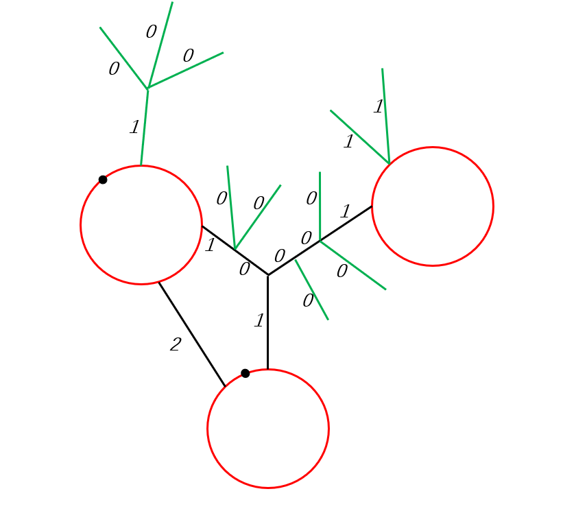
Figure 6: Structure of a ribbon graph: an example with leaves colored green

Except for Definition 3.9 (see Figure 6 for an example), we also need

Definition 5.1.

For any ribbon graph $\Upsilon$, let an inner edge $e\in\mathcal{E}_{int}(\Upsilon)$ and an inner vertex $v\in\mathcal{V}_{int}(\Upsilon)$.

• We call an edge $e$ a leaf if it will be deleted in the first step of Okounkov’s reduction. Otherwise, we call $e$ an excursive edge (excursion), if $e\in\mathcal{E}_{int}$ is not a leaf, that is, $e$ is on an excursion path of the reduced diagram in the sense of Section 2. Let $\mathcal{E}_{leaf},\mathcal{E}_{exc}$ be the set of all leaves and excursive edges in the inner edge set, one has another partition

  $$\mathcal{E}(\Upsilon)=\mathcal{E}_{b}(\Upsilon)\sqcup\mathcal{E}_{leaf}\sqcup\mathcal{E}_{exc}.$$ (5.1)

• Similarly, we can define a leafy vertex and an excursive vertex and have a partition

  $$\mathcal{V}(\Upsilon)=\mathcal{V}_{b}(\Upsilon)\sqcup\{\text{leafy vertices}\}\sqcup\{\text{excursion vectices}\}=:\mathcal{V}_{b}(\Upsilon)\sqcup\mathcal{V}_{leaf}\sqcup\mathcal{V}_{exc}.$$ (5.2)

Definition 5.2 (Couplings).

Let $\Upsilon$ be a ribbon graph. A coupling $\mathfrak{p}$ of $\Upsilon$ is a finite group of edges
$P_{1}=\{e_{1}^{(1)}=(x^{(1)}_{1},y^{(1)}_{1}),\dots,e_{p_{1}}^{(1)}=(x^{(1)}_{p_{1}},y^{(1)}_{p_{1}})\},\cdots,P_{l}=\{e_{1}^{(l)}=(x^{(l)}_{1},y^{(l)}_{1}),\dots,e_{p_{l}}^{(l)}=(x^{(l)}_{p_{l}},y^{(l)}_{p_{l}})\}$, where $p_{1},\dots,p_{l}\geq 2$, and $e^{(i)}_{j}$ $(1\leq i\leq l,1\leq j\leq p_{i})$ are distinct (directed) interior edges of $\Upsilon$. We call $P_{1},\dots,P_{l}$ blocks of $\mathfrak{p}$, and define the number of edges in $P_{i}$ as the length of $P_{i}$.

Roughly speaking, two or more edges $e_{i}=(x_{i},y_{i})\ (1\leq i\leq l)$ are coupled, which in fact means that one glues the these edges by viewing $x_{1}=\cdots=x_{l}$ and $y_{1}=\cdots=y_{l}$. Hence in the definition, for each $e^{(i)}_{j}$ in the coupling $\mathfrak{p}$ we firstly assign it with a order of its two endpoints $(x^{(i)}_{j},y^{(i)}_{j})$. We emphasize that it makes no sense to say that two or more undirected edges are coupled.

For any $\eta:V(\Upsilon)\to[N]$, values of $\eta$ induce a coupling on $V(\Upsilon)$ naturally. But many kinds of couplings can be negligible, except for the following three kinds as shown in Figure 7.

1. A 1-sided leafy edge coupled with another 1-sided leafy edge by identifying their boundary endpoints and inner vertices respectively. Denote such a set of coupling by $\mathfrak{p}_{1}$.

2. Length two excursions coupling by identifying the two boundary endpoints.

3. Two-sided edge couplings.

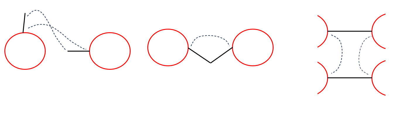
Figure 7: Three kinds of non-negligible couplings.

Hence, for the term contributing the main part, the coupling factor should be decoupled into three parts, corresponding to the above three kinds of couplings. Recalling the notations in Definition 3.9 and Definition 5.2, we introduce the following notations to characterize the three parts.

• For any set of (P1)-couplings $\mathfrak{p}_{1}$, set

  $$c(\eta,\mathfrak{p}_{1})= \prod_{\{e_{1},e_{2}\}\in\mathfrak{p}_{1}}1_{\{\eta(v^{i}_{e_{1}})=\eta(v^{i}_{e_{2}}),\eta(v^{b}_{e_{1}})=\eta(v^{b}_{e_{2}})\}}c(\eta,\{e_{1},e_{2}\})$$ (5.3)

  $$\times\prod_{\{e_{1},e_{2}\}\in\binom{\mathcal{E}_{1}(\Upsilon)\cap\mathcal{E}_{leaf}(\Upsilon)}{2}\backslash\mathfrak{p}_{1}}(1-1_{\{\eta(v^{i}_{e_{1}})=\eta(v^{i}_{e_{2}}),\eta(v^{b}_{e_{1}})=\eta(v^{b}_{e_{2}})\}}),$$

  where

  $$c(\eta,\{e_{1},e_{2}\})=\frac{\mathbb{E}\Big{[}|{W}_{\eta(v^{i}_{e_{1}})\eta(v^{b}_{e_{1}})}|^{4}\Big{]}}{\mathbb{E}\Big{[}({W}_{\eta(v^{i}_{e_{1}})\eta(v^{b}_{e_{1}})}^{\mathrm{GOE}})^{4}\Big{]}}.$$ (5.4)

• For $e_{1},e_{2}\in\mathcal{E}_{exc}(\Upsilon)\cap\mathcal{E}_{1}(\Upsilon)$, set

  $$c_{2,\Upsilon}(\eta)=\prod_{\{e_{1},e_{2}\}\in\binom{\mathcal{E}_{exc}(\Upsilon)\cap\mathcal{E}_{1}(\Upsilon)}{2}}1_{\{v^{i}_{e_{1}}=v^{i}_{e_{2}},\eta(v^{b}_{e_{1}})=\eta(v^{b}_{e_{2}})\}}c(\eta,\{e_{1},e_{2}\}),$$ (5.5)

  Note that the condition $1_{\{v^{i}_{e_{1}}=v^{i}_{e_{2}}\}}$ means that $e_{1},e_{2}$ are the edges on a two-step excursion, and $1_{\{\eta(v^{b}_{e_{1}})=\eta(v^{b}_{e_{2}})\}}$ means the values of $\eta$ on boundary vertices are same. Namely, one should take into account the fourth moment.

• Define

  $$c_{3,\Upsilon}(\eta):=\frac{\mathbb{E}[\prod_{\vec{e}=\vec{xy}\in\mathcal{E}_{2}(\Upsilon)}W_{\eta(x)\eta(y)}]}{\mathbb{E}[\prod_{\vec{e}=\vec{xy}\in\mathcal{E}_{2}(\Upsilon)}(W^{\rm GOE}_{\eta(x)\eta(y)})]}$$ (5.6)

  to measure the effect of (P3)-couplings.

• The main term from the regular couplings is defined as

  $$\mathcal{W}^{\mathrm{reg}}_{\Gamma,X}(k_{1},\dots,k_{s}):= \rho_{a}^{-k}\sum_{\Upsilon:\Phi(\Upsilon)=\Gamma}\sum_{\mathfrak{p}}\sum_{\eta:\mathcal{V}(\Upsilon)\to[N]}c(\eta,\mathfrak{p})c_{2,\Upsilon}(\eta)c_{3,\Upsilon}(\eta)$$ (5.7)

  $$\ \times\prod_{(x,y)\in\mathcal{E}_{int}(\Upsilon)}\sigma_{\eta(x)\eta(y)}^{2}\prod_{(z,w)\in\mathcal{E}_{b}(\Upsilon)}A_{\eta(z)\eta(w)}.$$

where the summation $\sum_{\mathfrak{p}}$ is over all (P1) couplings of the ribbon graph $\Upsilon$.

The first main result in this section is the following proposition that helps us removing other couplings.

Proposition 5.3.

Let $r$ be a fixed constant, if $k=\sum_{i=1}^{s}k_{i}$ is even and $k_{i}=[t_{i}/\sigma^{*}_{N}]$ with any fixed $t_{i}>0$ for $i=1,2,\dots,s$. Then, for any typical diagram $\Gamma$, as $N\to\infty$ we have

$$|\mathcal{W}_{\Gamma,X}(k_{1},\dots,k_{s})-\mathcal{W}^{\mathrm{reg}}_{\Gamma,X}(k_{1},\dots,k_{s})|=o(1).$$ (5.8)

Proof of Proposition 5.3.

Take $M=\lfloor\gamma^{-1}((r+1)\sigma_{N}^{*})^{-2}\rfloor$. To remove negligible parts we only need to consider the GOE case as shown in (3.89) that for any $G_{0}$, GOE bounds IRM.For the diagrams associated with GOE_M, the problem reduces to a counting/probability problem.

During the rest of the proof process, we consider a probabilistic model that uniformly taking all possible $\Upsilon$ with $\Phi(\Upsilon)=\Gamma$ and labeling $\eta:\mathcal{V}(\Upsilon)\rightarrow[M]$, let $\mathbb{P}$ be the probability measure. We also fix the number of boundary edges in our consideration. We show that the non-regular couplings are negligible by showing that their probability tends to $0$ case by case.

• Couplings with 0-sided edge. We consider two 0-sided edges coupling here. If the two edges share no common vertex. We first choose one endpoint of the two edges, saying $u,v$ and $\eta(u)=\eta(v)$. Since $u\neq v$, this reduces a probability $M^{-1}$($M$ available vertices in total). Then we choose the other endpoints, there are almost $d_{u}d_{v}$ ways to choose different vertices and reduce probability $M^{-1}$. If the two edges share a common vertex, saying $u=v$, we choose the other endpoints. This leads to a factor of $M^{-1}{d_{u}^{2}}$.

  $$\mathbb{P}(\text{2 0-sided edges couple})\leq\mathbb{E}\big{[}\sum_{u,v}\frac{d_{u}d_{v}}{M^{2}}+\sum_{u}\frac{d_{u}^{2}}{M}\big{]}\leq O(\frac{k^{2}}{M^{2}})+\frac{k}{M}\mathbb{E}\big{[}\frac{\sum_{u\in\mathcal{V}(\Upsilon)}d_{u}^{2}}{k}\big{]}\rightarrow 0.$$ (5.9)

  Here we have used the fact $\frac{1}{k}\mathbb{E}[\sum_{u\in\mathcal{V}(\Upsilon)}d_{u}^{2}]=O(1)$ in the last line by using results for vertex degree of random trees, see e.g. [OP09].

• Higher coupling of 1-sided edges. We show that the 6-th moment couplings are negligible. We choose three 1-side edges $e_{1},e_{2},e_{3}$ first. If they share no common inner vertex and are coupled, the number of free vertices must reduce at least $2$ by elaborating all possible situations. This leads to a $M^{-2}$ factor, and the total weight for this situation is $O({k^{3}}M^{-2})$.

  Now we consider the case the edges sharing some common inner vertex. Since we are considering the typical diagram, there is no interior vertex with degree $\geq 3$. Hence only two edges can share a common inner vertex and they come from a excursion with length 2 since they are all attached to boundary vertices. The couplings of excursions and 1-sided edges are treated latter.

• Coupling of 1-sided edges and excursions. For a fixed diagram $\Gamma$, the number of excursions is finite. We have already show that coupling with the inner edges are negligible, and the 1-side edges in excursions are finite, implying

  $$\mathbb{P}(\text{1-sided edges couple with excursions})$$ (5.10)

  $$\leq\mathbb{P}(\text{1-sided edges couple with 0-sided edge in excursions})$$

  $$+\mathbb{P}(\text{1-sided edges couple with 1-sided or 2-sided edge in excursions})$$

  We know that the first term tends to 0 from former argument and for the latter term, we have

  $$\mathbb{P}(\text{1-sided edges couple with 1/2-sided edge in excursions})$$ (5.11)

  $$\leq\mathbb{E}[\sum_{e_{1}\in\mathcal{E}_{1},e_{2}\in\mathcal{E}_{1}\cap\mathcal{E}_{exc}}1_{\{e_{1},e_{2}\text{ couple}\}}]\leq\frac{2k}{M}\#\{\text{excursions}\}\rightarrow 0.$$

The above arguments show that in the main term: (1) the 0-sided edges do not get into coupling. (2) The 1-sided edges only have pair couplings. (3) The 1-sided edges do not couple with excursions. These show that only regular couplings in Definition 5.2.

In a formal description, we have

$$|\mathcal{W}_{\Gamma,X}(k_{1},\dots,k_{s})-\mathcal{W}^{\mathrm{reg}}_{\Gamma,X}(k_{1},\dots,k_{s})|\leq|\mathcal{W}_{\Gamma,Y_{M}}(k_{1},\dots,k_{s})-\mathcal{W}^{\mathrm{reg}}_{\Gamma,Y_{M}}(k_{1},\dots,k_{s})|.$$ (5.12)

By the above discussions, with modifying some values in negligible couplings, we have

$$|\mathcal{W}_{\Gamma,Y_{M}}(k_{1},\dots,k_{s})-\mathcal{W}^{\mathrm{reg}}_{\Gamma,Y_{M}}(k_{1},\dots,k_{s})|=o(1).$$ (5.13)

This thus completes the proof of the proposition. ∎

The second main result is the following lemma making the regular term more viable.

Lemma 5.4.

For any typical diagram $\Gamma$, we have the following equation

$$\mathcal{W}^{\mathrm{reg}}_{\Gamma,X}(k_{1},\dots,k_{s})=\rho_{a}^{-k}\sum_{\Upsilon:\Phi(\Upsilon)=\Gamma}\sum_{\mathfrak{p}}\sum_{\eta:\mathcal{V}(\Upsilon)\to[N]}c_{2,\Upsilon}(\eta)c_{3,\Upsilon}(\eta)$$ (5.14)

$$~{}~{}~{}~{}\cdot\prod_{\{e_{1},e_{2}\}\in\mathfrak{p}}1_{\{\eta(v^{i}_{e_{1}})=\eta(v^{i}_{e_{2}}),\eta(v^{b}_{e_{1}})=\eta(v^{b}_{e_{2}})\}}(c(\eta,\{e_{1},e_{2}\})-1)\prod_{(x,y)\in\mathcal{E}_{int}(\Upsilon)}\sigma_{\eta(x)\eta(y)}^{2}\prod_{(z,w)\in\mathcal{E}_{b}(\Upsilon)}A_{\eta(z)\eta(w)}.$$

Here the summation $\sum_{\mathfrak{p}}$ is over all set of unordered pairs in $\mathcal{E}_{1}(\Upsilon)\cap\mathcal{E}_{leaf}(\Upsilon)$.

Proof of Lemma 5.4.

The proof is just a direct calculation.

$$\mathcal{W}^{\mathrm{reg}}_{\Gamma,X}(k_{1},\dots,k_{s})$$ (5.15)

$$= \rho_{a}^{-k}\sum_{\Upsilon:\Phi(\Upsilon)=\Gamma}\sum_{\mathfrak{p}_{1}}\sum_{\eta:\mathcal{V}(\Upsilon)\to[N]}c(\eta,\mathfrak{p}_{1})c_{2,\Upsilon}(\eta)c_{3,\Upsilon}(\eta)\prod_{(x,y)\in\mathcal{E}_{int}(\Upsilon)}\sigma_{\eta(x)\eta(y)}^{2}\prod_{(z,w)\in\mathcal{E}_{b}(\Upsilon)}A_{\eta(z)\eta(w)}$$

$$= \rho_{a}^{-k}\sum_{\Upsilon:\Phi(\Upsilon)=\Gamma}\sum_{\eta:\mathcal{V}(\Upsilon)\to[N]}c_{2,\Upsilon}(\eta)c_{3,\Upsilon}(\eta)\sum_{\mathfrak{p}_{1}}c(\eta,\mathfrak{p}_{1})\prod_{(x,y)\in\mathcal{E}_{int}(\Upsilon)}\sigma_{\eta(x)\eta(y)}^{2}\prod_{(z,w)\in\mathcal{E}_{b}(\Upsilon)}A_{\eta(z)\eta(w)}.$$

Recalling the definition of $c(\eta,\mathfrak{p}_{1})$ in (5.3), we sum over all possible (P1) couplings $\mathfrak{p}_{1}$ and get

$$\sum_{\mathfrak{p}_{1}}c(\eta,\mathfrak{p}_{1}) =\prod_{\{e_{1},e_{2}\}\in\binom{\mathcal{E}_{leaf}\cap\mathcal{E}_{1}}{2}}\Big{(}1_{\{\eta(v^{i}_{e_{1}})=\eta(v^{i}_{e_{2}}),\eta(v^{b}_{e_{1}})=\eta(v^{b}_{e_{2}})\}}c(\eta,\{e_{1},e_{2}\})$$ (5.16)

$$~{}~{}~{}~{}~{}~{}~{}~{}~{}~{}~{}~{}~{}~{}~{}~{}~{}~{}~{}~{}~{}~{}~{}~{}~{}~{}~{}~{}~{}~{}+1-1_{\{\eta(v^{i}_{e_{1}})=\eta(v^{i}_{e_{2}}),\eta(v^{b}_{e_{1}})=\eta(v^{b}_{e_{2}})\}}\Big{)}$$

$$=\sum_{\mathfrak{p}\subset\binom{\mathcal{E}_{leaf}\cap\mathcal{E}_{1}}{2}}\prod_{e=\{e_{1},e_{2}\}\in\mathfrak{p}}1_{\{\eta(v^{i}_{e_{1}})=\eta(v^{i}_{e_{2}}),\eta(v^{b}_{e_{1}})=\eta(v^{b}_{e_{2}})\}}(c(\eta,\{e_{1},e_{2}\})-1)$$

Here the sum over $\mathfrak{p}$ is over all set of pairs in the 1-sided edges.

∎

5.2 Diagram with leaves

To deal with the 1-sided edge coupling and to explore the relation between diagram function and limiting matrix $Z_{\beta}$, we introduce another key concept in the sub-Gaussian setting: leafy diagram. Roughly speaking, we treat the coupling 1-sided edges as the leaves attached to diagrams and their couplings become the couplings of these leaves. While for other leafy edges on $\Upsilon$, Based on (5.14), one can reduce these edge due to the double-stochastic property as we did in Section 2.

Definition 5.5 (Leafy diagram).

A leafy diagram $\Gamma_{l}=(\Gamma,\mathfrak{p})$ with respect to $\Gamma$ is composed of the following three parts:

• A (unnecessarily connected) diagram $\Gamma$ with $s$ faces.

• An (even) number of leaves attach to the boundary edges of $\Gamma$. These edges are named as leafy edges.

• The leaves are coupled by a set of pairs $\mathfrak{p}\subset\binom{E_{leaf}}{2}$, where all leaves occur in $\mathfrak{p}$.

Similar to Definition 5.2, one need the following notations to spell out structures of a leafy diagram.

1. We classify the edge set $E(\Gamma_{l})$ into three parts: excursion edges ${E}_{exc}$, leafy edges $E_{leaf}$ and boundary edges $E_{b}$.

   $$E(\Gamma_{l})={E}_{exc}(\Gamma_{l})\sqcup E_{b}(\Gamma_{l})\sqcup E_{leaf}(\Gamma_{l}).$$ (5.17)

2. For each leafy edge $e$, denote by $v^{b}_{e}$ its boundary endpoint and by $v^{i}_{e}$ the interior endpoint. Note that the coupling $\mathfrak{p}$ induces a pairing of $\{v^{b}_{e}:e\in E_{leaf}\}$ and a pairing of $\{v^{i}_{e}:e\in E_{leaf}\}$. Denote the quotient set as $V_{leaf}^{b}=\{v^{b}_{e}:e\in E_{leaf}\}/\sim$ and $V_{leaf}^{i}=\{v^{i}_{e}:e\in E_{leaf}\}/\sim$.

3. Again, $V_{b}(\Gamma_{l})$ denotes the set of all boundary vertices $\Gamma_{l}$.

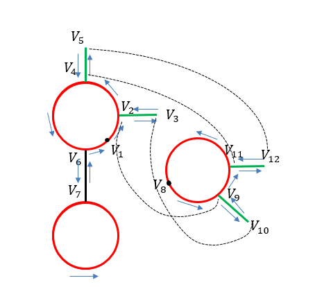
Figure 8: An example of leafy diagram(couplings are drawn as dotted lines)

Now one can use the Okounkov’s contraction to classify ribbon graphs to diagrams. Formally, we construct the contraction map

$$\Phi_{l}:\Big{\{}(\Upsilon,\mathfrak{p}):\mathfrak{p}\subset\binom{\mathcal{E}_{leaf}\cap\mathcal{E}_{1}}{2}\Big{\}}\longrightarrow\ \{\Gamma_{l}:\text{all leafy diagrams}\}$$ (5.18)

defined by removing all edges in $\mathcal{E}_{leaf}(\Upsilon)$ but not in $\mathfrak{p}$.

To be precise, any (P1) type coupling of 1-side edges in $\Upsilon$ naturally gives a leafy diagram with coupling by removing all trees. Conversely, a leafy diagram with $\mathfrak{p}_{1}$ type coupling reconstructs $\Upsilon$ by adding the trees. Given a leafy diagram, we sum up all possible trees and get the resulting diagram function.

Definition 5.6 (Leafy diagram functions).

For any leafy diagram $\Gamma_{l}$, the leafy diagram function associated to $\Gamma_{l}$ is defined to be

$$\mathcal{W}^{\mathrm{leaf}}_{\Gamma_{l},X}(k_{1},\dots,k_{s}): =\rho_{a}^{-k}\sum_{(\Upsilon,\mathfrak{p}):\Phi_{l}(\Upsilon,\mathfrak{p})=\Gamma_{l}}\sum_{\eta:\mathcal{V}(\Upsilon)\to[N]}\prod_{e=\{e_{1},e_{2}\}\in\mathfrak{p}}1_{\{\eta(v^{i}_{e_{1}})=\eta(v^{i}_{e_{2}}),\eta(v^{b}_{e_{1}})=\eta(v^{b}_{e_{2}})\}}$$ (5.19)

$$~{}~{}~{}~{}\cdot(c(\eta,\{e_{1},e_{2}\})-1)c_{2,\Upsilon}(\eta)c_{3,\Upsilon}(\eta)\prod_{(x,y)\in\mathcal{E}_{int}(\Upsilon)}\sigma_{\eta(x)\eta(y)}^{2}\prod_{(z,w)\in\mathcal{E}_{b}(\Upsilon)}A_{\eta(z)\eta(w)}.$$

Let $\Gamma_{l}=(\Gamma,\mathfrak{p})$ be the leafy diagrams corresponding to diagram $\Gamma$, by definition we see

$$\mathcal{W}^{\mathrm{reg}}_{\Gamma,X}(k_{1},\dots,k_{s})=\sum_{\Gamma_{l}=(\Gamma,\mathfrak{p})}\mathcal{W}^{\mathrm{leaf}}_{\Gamma_{l},X}(k_{1},\dots,k_{s}).$$ (5.20)

Similar to discussions in Section 2, the leafy diagram functions can be simplified as follows.

Proposition 5.7.

For any leafy diagram, we have

$$\mathcal{W}^{\mathrm{leaf}}_{\Gamma_{l},X} (k_{1},\dots,k_{s})=\rho_{a}^{-k}\sum_{\begin{subarray}{c}(n_{e})_{e\in E(\Gamma)}\\ n|_{E_{leaf}=1}\end{subarray}}\sum_{\eta:V_{b}\to[r]}\sum_{\eta:V_{\rm leaf}^{i}\to[N]}\prod_{e=(x,y)\in E_{int}}p_{n_{e}}(\eta(x),\eta(y))\prod_{e=(z,w)\in E_{b}}A^{n_{e}}_{\eta(x)\eta(y)}$$ (5.21)

$$\cdot\prod_{j=1}^{s}\binom{k_{j}}{\frac{k_{j}-\sum_{e\in\partial D_{j}}n_{e}}{2}}\prod_{\{e_{1},e_{2}\}\in\mathfrak{p}}1_{\{\eta(v^{i}_{e_{1}})=\eta(v^{i}_{e_{2}}),\eta(v^{b}_{e_{1}})=\eta(v^{b}_{e_{2}})\}}(c(\eta,\{e_{1},e_{2}\})-1)c_{2,\Gamma_{l}}(\eta,\vec{n})c_{3,\Gamma_{l}}(\eta,\vec{n}).$$

where the two coupling factors

$$c_{2,\Gamma_{l}}(\eta,\vec{n}):=\prod_{\begin{subarray}{c}\{e_{1},e_{2}\}\in\binom{E_{exc}}{2}\\ n_{e_{1}}=n_{e_{2}}=1\end{subarray}}1_{\{v^{i}_{e_{1}}=v^{i}_{e_{2}},\eta(v^{b}_{e_{1}})=\eta(v^{b}_{e_{2}})\}}\frac{\mathbb{E}\Big{[}|{W}_{\eta(v^{i}_{e_{1}})\eta(v^{b}_{e_{1}})}|^{4}\Big{]}}{\mathbb{E}\Big{[}({W}_{\eta(v^{i}_{e_{1}})\eta(v^{b}_{e_{1}})}^{\mathrm{GOE}})^{4}\Big{]}}\prod_{\begin{subarray}{c}e\in E_{exc}\\ n_{e}=2\end{subarray}}1_{\{\eta(x)=\eta(y)\}}\sum_{z}\sigma_{\eta(x)z}^{4}\frac{\mathbb{E}[|W_{\eta(x)z}|^{4}]}{\mathbb{E}[|W^{\rm GOE}_{\eta(x)z}|^{4}]}$$ (5.22)

$$c_{3,\Gamma_{l}}(\eta,\vec{n}):=\frac{\mathbb{E}[\prod_{\vec{e}=\vec{xy}\in E_{2}:n_{e}=1}W_{\eta(x)\eta(y)}]}{\mathbb{E}[\prod_{\vec{e}=\vec{xy}\in E_{2}:n_{e}=1}W^{\rm GOE}_{\eta(x)\eta(y)}]}.$$ (5.23)

measures the effect of (P2) couplings and (P3) couplings respectively.

Proof.

We count the pre-images. Again, for any non-leaf edge $e\in E(\Gamma_{l})\backslash E_{\rm leaf}$, denote $n_{e}$ be the number of segments of $\Upsilon$ on the edge $e$. Note that at this time the number of deleted divalent vertex on this edge is $n_{e}-1$.

Similar to the Gaussian case, one sees that the total number of all possible trees on the $j$-th face is

$$\sum_{u_{1}+\cdots u_{n_{j}}=(k_{j}-n_{j})/2,\ u_{i}\geq 0}(2u_{1}+1)\prod_{i=1}^{n_{j}}C_{u_{i}}=\binom{k_{j}}{\frac{1}{2}(k_{j}-n_{j})},$$ (5.24)

here $n_{j}=\sum_{e\in\partial D_{j}}n_{e}$ is the summation of $n_{e}$ for $e\in\partial D_{j}$.

Noting that the coupling factor $c_{2,\Gamma_{l}}(\eta,\vec{n})$, $c_{3,\Gamma_{l}}(\eta,\vec{n})$ coincide with $c_{2,\Upsilon}(\eta)$ and $c_{3,\Upsilon}(\eta)$ respectively. This finishes the proof of Proposition 5.7. ∎

5.3 Limits of leafy diagram functions

The scope of this section is to prove Proposition 5.9, obtaining the limit behaviour of leafy diagram functions.

Definition 5.8.

1. A leafy diagram $\Gamma_{l}=(\Gamma,\mathfrak{p})$ is called typical if $\Gamma$ is a typical diagram, the pairing $\mathfrak{p}$ is a (P1)-coupling, and each $(v_{e}^{b})_{e\in E_{leaf}}$ are distinct.

2. For a typical leafy diagram $\Gamma_{l}$, define the limiting diagram function of $\Gamma_{l}$ as

   $$w_{\Gamma_{l}}(t_{1},\dots,t_{s}):=\sum_{\eta:V_{b}\to[r]}\sum_{J\subset E_{int}}\prod_{j=1}^{s}\frac{(t_{j}\sigma_{a})^{|E_{b,j}|-1}}{(|E_{b,j}|-1)!}\prod_{x\in V_{leaf}^{b}}\Big{(}\frac{1}{3}\tau_{\eta(x)}-\chi_{\eta(x)}\Big{)}\prod_{(z,w)\in E_{b}}(Q_{\beta}Q_{\beta}^{*})_{\eta(z)\eta(w)}\\ \times c_{3,\Gamma_{l}}(\eta,J)a^{-|E_{b}|+s}\prod_{(x,y)\in J}\Big{(}g_{\eta(x)\eta(y)}+\frac{1}{3}\tau_{\eta(x)}\delta_{\eta(x)\eta(y)}\Big{)}\prod_{(x,y)\in E_{int}\backslash J}\tilde{\sigma}^{2}_{\eta(x)\eta(y)},$$ (5.25)

where the coupling factor

$$c_{3,\Gamma_{l}}(\eta,J):=\frac{\mathbb{E}[\prod_{\vec{e}=\vec{xy}\in J}W_{\eta(x)\eta(y)}]}{\mathbb{E}[\prod_{\vec{e}=\vec{xy}\in J}W^{\rm GOE}_{\eta(x)\eta(y)}]}$$ (5.26)

measures the effect of 2-side edge couplings.

Proposition 5.9.

Assume that $k_{i}=\lfloor t_{i}/\sigma_{N}^{*}\rfloor$ with fixed $t_{i}>0$ for $i=1,\ldots,s$. Then for any non-typical leafy diagram $\Gamma_{l}$ such that for any $j$, $E_{b,j}(\Gamma_{l})\neq\emptyset$, we have

$$\lim\limits_{N\rightarrow\infty}\mathcal{W}^{\mathrm{leaf}}_{\Gamma_{l},X}(k_{1},\dots,k_{s})=0.$$ (5.27)

while for any typical leafy diagram $\Gamma_{l}$

$$\lim\limits_{N\rightarrow\infty}\mathcal{W}^{\mathrm{leaf}}_{\Gamma_{l},X}(k_{1},\dots,k_{s})=w_{\Gamma_{l}}(t_{1},\dots,t_{s}).$$ (5.28)

To complete the proof of Proposition 5.9, we proceed in four steps by stating four propositions, in which proofs of Proposition 5.10, Proposition 5.11 and Proposition 5.12 are given in Appendix B, Appendix C and Appendix D.

Step 1: Couplings in $\mathfrak{p}$.

Proposition 5.10.

With $\mathcal{W}^{\mathrm{leaf}}_{\Gamma_{l},X}(k_{1},\dots,k_{s})$ defined in (5.21) and with the same assumptions in Proposition 5.9, we have

$$\lim\limits_{N\rightarrow\infty}|\mathcal{W}^{\mathrm{leaf}}_{\Gamma_{l},X}(k_{1},\dots,k_{s})-\mathcal{W}_{\Gamma_{l},X}^{\rm I}(k_{1},\dots,k_{s})|=0,$$ (5.29)

where

$$\mathcal{W}_{\Gamma_{l},X}^{\rm I}(k_{1},\dots,k_{s}):=\rho_{a}^{-k}\sum_{\begin{subarray}{c}(n_{e})_{e\in E(\Gamma)}\\ n|_{E_{leaf}=1}\end{subarray}}\sum_{\eta:V_{b}\to[r]}c_{2,\Gamma_{l}}(\eta,\vec{n})c_{3,\Gamma_{l}}(\eta,\vec{n})\prod_{e=(x,y)\in E_{exc}}p_{n_{e}}(\eta(x),\eta(y))\\ \times(\sigma_{N}^{*})^{2|\mathfrak{p}|}\prod_{j=1}^{s}\binom{k_{j}}{\frac{k_{j}-\sum_{\partial D_{j}}n_{e}}{2}}\prod_{e=(z,w)\in E_{b}}A^{n_{e}}_{\eta(x)\eta(y)}\prod_{x\in V_{leaf}^{b}}\Big{(}\frac{a^{2}}{3}\tau_{\eta(x)}-a^{2}\chi_{\eta(x)}\Big{)}.$$ (5.30)

Step 2: Removing smaller eigenvalues.

We need to handle the eigenvalues of $A$ less than $a$ and to eliminate their interference in the fluctuation.

Proposition 5.11.

With the same assumptions in Proposition 5.9, we have

$$\lim\limits_{N\rightarrow\infty}|\mathcal{W}_{\Gamma_{l}}^{{\rm I}}(k_{1},\dots,k_{s})-\mathcal{W}_{\Gamma_{l}}^{{\rm I},=a}(k_{1},\dots,k_{s})|=0,$$ (5.31)

where

$$\mathcal{W}_{\Gamma_{l}}^{{\rm I},=a}(k_{1},\dots,k_{s}):=\rho_{a}^{-k}\sum_{\begin{subarray}{c}(n_{e})_{e\in E(\Gamma)}\\ n|_{E_{leaf}=1}\end{subarray}}\sum_{\eta:V_{b}\to[r]}c_{2,\Gamma_{l}}(\eta,\vec{n})c_{3,\Gamma_{l}}(\eta,\vec{n})\prod_{e=(x,y)\in E_{exc}}p_{n_{e}}(\eta(x),\eta(y))\\ \times(\sigma_{N}^{*})^{2|\mathfrak{p}|}\prod_{j=1}^{s}\binom{k_{j}}{\frac{k_{j}-\sum_{\partial D_{j}}n_{e}}{2}}\prod_{e=(z,w)\in E_{b}}\hat{A}^{n_{e}}_{\eta(x)\eta(y)}\prod_{x\in V_{leaf}^{b}}\Big{(}\frac{a^{2}}{3}\tau_{\eta(x)}-a^{2}\chi_{\eta(x)}\Big{)}.$$ (5.32)

Step 3: Enumerating trees.

Proposition 5.12.

With the same assumptions in Proposition 5.9, we have

$$\lim\limits_{N\rightarrow\infty}|\mathcal{W}^{{\rm I},=a}_{\Gamma_{l},X}(k_{1},\dots,k_{s})-\mathcal{W}_{\Gamma_{l},X}^{\rm II}(k_{1},\dots,k_{s})|=0,$$ (5.33)

where

$$\mathcal{W}^{\rm II}_{\Gamma_{l},X}(k_{1},\dots,k_{s}):=\rho_{a}^{-k}\sum_{\eta:V_{b}\to[r]}\sum_{(n_{e})_{e\in{E}_{exc}}}c_{2,\Gamma_{l}}(\eta,\vec{n})c_{3,\Gamma_{l}}(\eta,\vec{n})a^{-4|\mathfrak{p}|}\prod_{x\in V_{leaf}^{b}}\Big{(}\frac{a^{2}}{3}\tau_{\eta(x)}-a^{2}\chi_{\eta(x)}\Big{)}\\ \times\prod_{e=(z,w)\in E_{b}}(Q_{\beta}Q_{\beta}^{*})_{\eta(z)\eta(w)}(\sigma_{N}^{*})^{2|\mathfrak{p}|}\prod_{j=1}^{s}\Big{(}\frac{(k_{j}\sigma_{a})^{|E_{b,j}|-1}}{(|E_{b,j}|-1)!}\Big{)}\prod_{e=(x,y)\in E_{int}}p_{n_{e}}(\eta(x),\eta(y))\frac{1}{a^{2n_{e}}},$$ (5.34)

and recall that

$$\sigma_{a}:=\frac{a^{2}-1}{a^{2}+1}.$$ (5.35)

Step 4: Limiting diagram functions.

Proposition 5.13.

Let $\mathcal{W}^{\rm II}_{\Gamma_{l},X}$ be given in (5.34) and $w_{\Gamma_{l}}$ be given in Definition 5.8, with the same assumptions in Proposition 5.9, we have

$$\lim\limits_{N\rightarrow\infty}\mathcal{W}^{\rm II}_{\Gamma_{l},X}(k_{1},\dots,k_{s})=w_{\Gamma_{l}}(t_{1},\dots,t_{s}).$$ (5.36)

Proof of Proposition 5.13.

We deal with the term $\sum_{n_{e}:e\in E_{int}}$ and study the excursion coupling factors $c_{2,\Gamma_{l}}(\eta,\vec{n})$ and $c_{3,\Gamma_{l}}(\eta,\vec{n})$ carefully.As mentioned before, for the excursion edge $e\in E_{int}$, one should consider the enumeration of 2-sided edges in both the cases of $n_{e}=1$ and $n_{e}\geq 2$ separately. To be precise, rewrite the summation of $n_{e}$ as

$$\sum_{n_{e}:e\in E_{exc}}=\sum_{J\subset{E}_{exc}}\sum_{n_{e}\geq 2:e\in J}$$ (5.37)

which means for $e\in{E}_{exc}\backslash J$, $n_{e}=1$.

For the excursion edges with length $\geq 2$, we calculate as follows

$$\sum_{(n_{e})_{e\in J}}c_{2,\Gamma_{l}}(\eta,\vec{n})\Big{(}\prod_{e=(x,y)\in J}p_{n_{e}}(\eta(x),\eta(y))\frac{1}{a^{2n_{e}}}\Big{)}$$ (5.38)

$$= \prod_{e=(x,y)\in J}\Big{(}\sum_{n_{e}\geq 2}p_{n_{e}}(\eta(x),\eta(y))\frac{1}{a^{2n_{e}}}-p_{2}(\eta(x),\eta(y))\delta_{\eta(x)\eta(y)}a^{-4}+\delta_{\eta(x)\eta(y)}a^{-4}\sum_{z}\sigma_{\eta(x)z}^{4}\frac{\mathbb{E}[|W_{\eta(x)z}|^{4}]}{\mathbb{E}[|W^{\rm GOE}_{\eta(x)z}|^{4}]}$$

$$= \sigma_{N}^{*-2|J|}(1+o(1))\prod_{e=(x,y)\in J}\Big{(}g_{\eta(x)\eta(y)}a^{-2}+\frac{1}{3a^{2}}\tau_{\eta(x)}\delta_{\eta(x)\eta(y)}\Big{)}.$$

While for the length-1 excursions (=2-side edges), we see

$$c_{3,\Gamma_{l}}(\eta,\vec{n})\prod_{e=(x,y)\in{E}_{exc}\backslash J}p_{1}(\eta(x),\eta(y))\frac{1}{a^{2}}=c_{3,\Gamma_{l}}(\eta,J)\prod_{e=(x,y)\in{E}_{exc}\backslash J}\widetilde{\sigma}^{2}_{(\eta(x),\eta(y))}\frac{1}{a^{2}}$$ (5.39)

Hence,

$$\mathcal{W}_{\Gamma_{l}}^{\rm II}(k_{1},\dots,k_{s})\sim\sum_{\eta:V_{b}\to[r]}\sum_{J\subset{E}_{exc}}a^{-4|\mathfrak{p}|-2|E_{exc}|}c_{3,\Gamma_{l}}(\eta,J)\prod_{x\in V_{leaf}^{b}}\Big{(}\frac{a^{2}}{3}\tau_{\eta(x)}-a^{2}\chi_{\eta(x)}\Big{)}\prod_{j=1}^{s}\frac{(t_{j}\sigma_{a})^{|E_{b,j}|-1}}{(|E_{b,j}|-1)!}\\ \times\prod_{(z,w)\in E_{b}}(Q_{\beta}Q_{\beta}^{*})_{\eta(z)\eta(w)}\prod_{e=(x,y)\in J}\Big{(}g_{\eta(x)\eta(y)}+\frac{1}{3}\tau_{\eta(x)}\delta_{\eta(x)\eta(y)}\Big{)}\prod_{e=(x,y)\in{E}_{exc}\backslash J}\tilde{\sigma}^{2}_{\eta(x)\eta(y)}\\ \times\sigma_{N}^{*-|E_{b}|+s+|E_{\rm leaf}|+2|E_{int}|}.$$ (5.40)

We now claim that for any leafy diagram $\Gamma_{l}$,

$$2|E_{int}(\Gamma_{l})|+2|\mathfrak{p}|-2|V_{int}|-|E_{b}(\Gamma_{l})|+s\geq 0.$$ (5.41)

and the equality holds if the diagram $\Gamma_{l}$ is typical.

In fact, in each step, remove a coupling of $\Gamma_{l}$, we see the above term descend with the operation. At the finial step we get the underlying diagram $\Gamma$, hence

$$2|E_{int}(\Gamma_{l})|+2|\mathfrak{p}|-2|V_{int}|-|E_{b}(\Gamma_{l})|+s\geq 2|E_{int}(\Gamma)||-2|V_{int}(\Gamma)|-|E_{b}(\Gamma)|+s\geq 0$$ (5.42)

Here the last inequality we use Lemma 2.9 for $\Gamma$.

Hence, For any non-typical diagram $\Gamma_{l}$,

$$\mathcal{W}_{\Gamma_{l}}^{\rm II}(k_{1},\dots,k_{s})=o(1).$$ (5.43)

And rewriting the power of $a$ as

$$a^{-4|\mathfrak{p}|-2|E_{exc}+2|V^{b}_{leaf}|}=a^{-2|\mathfrak{p}|-2|E_{exc}|}=a^{-|E_{b}|+s},$$ (5.44)

we obtain that for any typical diagram $\Gamma_{l}$,

$$\mathcal{W}_{\Gamma_{l}}^{\rm II}(k_{1},\dots,k_{s})\sim w_{\Gamma_{l}}(t_{1},\dots,t_{s}).$$ (5.45)

This finishes the proof of Proposition 5.13. ∎

Now we are ready to complete the proof of Proposition 5.9.

Proof of Proposition 5.9.

Combine Proposition 5.10-5.13 and we can easily complete the proof of Proposition 5.9. ∎

Remark 5.1.

Same discussions also hold in the Hermitian case with slight modifications.

• In the Hermitian case, $\mathbb{E}[W_{ij}^{2}]=0$, while $\mathbb{E}[|W_{ij}|^{2}]=1$. Hence for any uncoupled edge, the two directions must be opposite. Specifically, let $1_{\rm op}(e)$ be the indicate function of this event, then the regular part of diagram function is defined as

  $$\mathcal{W}^{\mathrm{reg}}_{\Gamma,X}(k_{1},\dots,k_{s}):= \rho_{a}^{-k}\sum_{\Upsilon:\Phi(\Upsilon)=\Gamma}\sum_{\mathfrak{p}}\sum_{\eta:\mathcal{V}(\Upsilon)\to[N]}c(\eta,\mathfrak{p})c_{2,\Upsilon}(\eta)c_{3,\Upsilon}(\eta)c_{4,\Upsilon}(\eta)$$ (5.46)

  $$\ \times\prod_{(x,y)\in\mathcal{E}_{int}(\Upsilon)}\sigma_{\eta(x)\eta(y)}^{2}\prod_{(z,w)\in\mathcal{E}_{b}(\Upsilon)}A_{\eta(z)\eta(w)}.$$

  where

  $$c_{4,\Upsilon}(\eta)=\prod_{e\in\mathcal{E}_{int}:\text{ uncoupled}}1_{\text{op}}(e).$$ (5.47)

  Similarly, the for any leafy diagram, the limiting diagram function is defined as

  $$w_{\Gamma_{l}}(t_{1},\dots,t_{s}):=\sum_{\eta:V_{b}\to[r]}\sum_{J\subset E_{int}}\prod_{j=1}^{s}\frac{(t_{j}\sigma_{a})^{|E_{b,j}|-1}}{(|E_{b,j}|-1)!}\prod_{x\in V_{leaf}^{b}}\Big{(}\frac{1}{3}\tau_{\eta(x)}-\chi_{\eta(x)}\Big{)}\prod_{(z,w)\in E_{b}}(Q_{2}Q_{2}^{*})_{\eta(z)\eta(w)}\\ \times c_{3,\Gamma_{l}}(\eta,J)a^{-|E_{b}|+s}\prod_{e=(x,y)\in J}\Big{(}g_{\eta(x)\eta(y)}1_{\rm op}(e)+\frac{1}{3}\tau_{\eta(x)}\delta_{\eta(x)\eta(y)}\Big{)}\prod_{(x,y)\in E_{int}\backslash J}\tilde{\sigma}^{2}_{\eta(x)\eta(y)},$$ (5.48)

• With $\mathcal{W}^{\mathrm{reg}}_{\Gamma,X}(k_{1},\dots,k_{s})$ defined in (5.46), Proposition 5.3 holds in the Hermitian case without modification since GOE also dominates Hermitian IRM.

• With $\mathcal{W}^{\mathrm{reg}}_{\Gamma,X}(k_{1},\dots,k_{s})$ defined in (5.46), the contraction map defined in (5.18) and Proposition 5.7 holds respectively since for each leaves of $\Upsilon$, the two directions associated with it are always opposite.

• With $w_{\Gamma_{l}}(t_{1},\dots,t_{s})$ defined in (5.48), Proposition 5.9 still holds. Since, roughly speaking, the extra coupling factor does not depend on (P2) couplings, (P3) couplings and tree counting.

5.4 Proof of Theorem 1.3

Theorem 5.14.

With the same notations and assumptions as in Theorem 1.3, let $k_{i}=\lfloor t_{i}/\sigma_{N}^{*}\rfloor$ with $t_{i}>0$, as $N\to\infty$ one has

$$\rho_{a}^{-k}\mathbb{E}\big{[}\prod_{j=1}^{s}\mathrm{Tr}X^{k_{j}}\big{]}\sim\sum_{\Gamma_{l}}w_{\Gamma_{l}}(t_{1},\dots,t_{s})$$ (5.49)

where the summation $\sum_{\Gamma_{l}}$ is over all typical leafy diagrams.

Proof of Theorem 5.14.

We claim that

$$\rho_{a}^{-k}\mathbb{E}[\prod_{j=1}^{s}\mathrm{Tr}X^{k_{j}}]\sim\rho_{a}^{-k}\mathbb{E}[\prod_{j=1}^{s}(\mathrm{Tr}X^{k_{j}}-\mathrm{Tr}H^{k_{j}})].$$ (5.50)

In fact, we have an expansion

$$\mathbb{E}[\prod_{j=1}^{s}\mathrm{Tr}X^{k_{j}}]-\mathbb{E}[\prod_{j=1}^{s}(\mathrm{Tr}X^{k_{j}}-\mathrm{Tr}H^{k_{j}})]=\sum_{\begin{subarray}{c}J\subset[s]\\ J\neq\emptyset\end{subarray}}(-1)^{|J|}\mathbb{E}\Big{[}\prod_{j\in J}\mathrm{Tr}H^{k_{j}}\prod_{j\notin J}\mathrm{Tr}X^{k_{j}}\Big{]}.$$ (5.51)

Hence, to prove the claim, it is enough to show that any non-empty $J\subset[s]$ one has

$$\lim_{N\to\infty}\rho_{a}^{-k}\mathbb{E}\Big{[}\prod_{j\in J}\mathrm{Tr}H^{k_{j}}\prod_{j\notin J}\mathrm{Tr}X^{k_{j}}\Big{]}=0.$$ (5.52)

We first prove (5.52) for $s=1$. By (4.4) and (4.5), noting the assumption $\sigma_{N}^{*}\log N\to 0$, we obtain

$$\rho_{a}^{-k}\mathbb{E}\Big{[}\mathrm{Tr}H^{k}\Big{]}\leq C\rho_{a}^{-k}Ne^{Ck^{3}(\sigma_{N}^{*})^{4}}\rightarrow 0.$$ (5.53)

Now we prove (5.52) for $s\geq 2$. By using Hölder inequality

$$\left|\mathbb{E}[\prod_{i=1}^{s}\xi_{i}]\right|\leq\prod_{i=1}^{s}\left(\mathbb{E}[|\xi_{i}|^{s}]\right)^{1/s},$$ (5.54)

we see

$$\rho_{a}^{-k}\mathbb{E}\Big{[}\prod_{j\in J}\mathrm{Tr}H^{k_{j}}\prod_{j\notin J}\mathrm{Tr}X^{k_{j}}\Big{]}\leq\prod_{j\in J}\left(\mathbb{E}\Big{[}\mathrm{Tr}(\rho_{a}^{-k_{j}}H^{k_{j}})^{s}\Big{]}\right)^{1/s}\prod_{j\notin J}\left(\mathbb{E}\Big{[}\mathrm{Tr}(\rho_{a}^{-k_{j}}X^{k_{j}})^{s}\Big{]}\right)^{1/s}.$$ (5.55)

By using Hölder inequality again but for eigenvalues we see for any $N\times N$ Hermitian matrix $L$, and any even number $k$

$$(\mathrm{Tr}L^{k})^{s}=(\sum_{i=1}^{N}\lambda_{i}^{k})^{s}\leq N^{s-1}\sum_{i=1}^{N}|\lambda_{i}|^{ks}=N^{s-1}\mathrm{Tr}L^{ks}.$$ (5.56)

Combining with (5.53), we have the following upper bound for the terms involving $H$

$$\prod_{j\in J}\left(\mathbb{E}\Big{[}\mathrm{Tr}(\rho_{a}^{-k_{j}}H^{k_{j}})^{s}\Big{]}\right)^{1/s}\leq N^{|J|}\prod_{j\in J}\left(\mathbb{E}[\mathrm{Tr}(\rho_{a}^{-1}H)^{sk_{j}}]\right)^{1/s}\leq C^{|J|}N^{2|J|}\prod_{j\in J}\Big{(}\frac{2}{\rho_{a}}\Big{)}^{sk_{j}}.$$ (5.57)

And combining (5.56), we get

$$\prod_{j\notin J}\mathbb{E}\Big{[}\mathrm{Tr}(\rho_{a}^{-k_{j}}X^{k_{j}})^{s}\Big{]}^{1/s}\leq N^{s-|J|}\prod_{j\notin J}\mathbb{E}[\mathrm{Tr}(\rho_{a}^{-1}X)^{sk_{j}}]^{1/s}\leq N^{s-|J|}C.$$ (5.58)

Hence for any $J\neq\emptyset$,

$$\rho_{a}^{-k}\mathbb{E}\Big{[}\prod_{j\in J}\mathrm{Tr}H^{k_{j}}\prod_{j\notin J}\mathrm{Tr}X^{k_{j}}\Big{]}\leq N^{s}\prod_{j\in J}\Big{(}\frac{2}{\rho_{a}}\Big{)}^{sk_{j}}C^{s}\rightarrow 0.$$ (5.59)

This finishes the proof of (5.52) implying the claim.

Now we combine the claim with Proposition 2.8, Proposition 5.3 and (2.16), to see

$$\rho_{a}^{-k}\mathbb{E}[\prod_{j=1}^{s}\mathrm{Tr}X^{k_{j}}] =\sum_{\Gamma:E_{b},j(\Gamma)\neq\emptyset\text{ for each }j}\mathcal{W}_{\Gamma}(k_{1},\dots,k_{s})+o(1)$$ (5.60)

$$=\sum_{\Gamma:E_{b},j(\Gamma)\neq\emptyset\text{ for each }j}\mathcal{W}^{\rm reg}_{\Gamma}(k_{1},\dots,k_{s})+o(1).$$

Here we use the DCT to make sure that the summation with $\Gamma$ and the limit of $N$ are exchangeable, hence one has ignored the contribution of the irregular part. The dominating function is given by Theorem 3.2. Now we consider

$$\sum_{\Gamma:E_{b},j(\Gamma)\neq\emptyset\text{ for each }j}\mathcal{W}^{\rm reg}_{\Gamma}(k_{1},\dots,k_{s}).$$ (5.61)

We expand (5.61) in terms of leafy diagrams. Formally, by (5.20) we see

$$\sum_{\Gamma:E_{b},j(\Gamma)\neq\emptyset\text{ for each }j}\mathcal{W}^{\rm reg}_{\Gamma}(k_{1},\dots,k_{s})=\sum_{\Gamma_{l}:E_{b},j(\Gamma_{l})\neq\emptyset\text{ for each }j}\mathcal{W}^{\rm leaf}_{\Gamma_{l}}(k_{1},\dots,k_{s}).$$ (5.62)

Now, by Proposition 5.9, we use DCT again (the dominating function is given by the Gaussian case again) to see

$$\lim_{N\to\infty}\sum_{\Gamma_{l}:E_{b},j(\Gamma_{l})\neq\emptyset\text{ for each }j}\mathcal{W}^{\rm leaf}_{\Gamma_{l}}(k_{1},\dots,k_{s})=\sum_{\Gamma_{l}}w_{\Gamma_{l}}(t_{1},\dots,t_{s}).$$ (5.63)

Combining (5.60), (5.62) and (5.63), we thus have completed the proof. ∎

Next, we need to compare the summation over typical leafy diagrams in Theorem 5.14 with the corresponding moments of $Z_{\beta}$ defined in (1.20). By using the similar argument in Proposition 2.8 we have the following lemma.

Lemma 5.15.

For $\beta=1,2$, let $Z_{\beta}$ be the random matrix in (1.20), then for positive integers $e_{1},\dots,e_{s}$, we have a diagram expansion

$$\prod_{j=1}^{s}\frac{1}{e_{j}!}\Big{(}\frac{t_{j}(a^{2}-1)}{a(a^{2}+1)}\Big{)}^{e_{j}}\mathbb{E}\big{[}\prod_{j=1}^{s}\mathrm{Tr}Z_{\beta}^{e_{j}}\big{]}=\sum_{\begin{subarray}{c}\Gamma_{l}{\rm\ typical}\\ |E_{b,j}(\Gamma)|=e_{j}+1\end{subarray}}w_{\Gamma_{l}}(t_{1},\dots,t_{s}).$$ (5.64)

Proof of Lemma 5.15.

In fact we only need to prove the lemma under the assumption $\tau_{i}\geq 3\chi_{i}$ for every $1\leq i\leq r$. For the general case, noting that both sides are polynomials of $\tau_{i}$, we can extend the equality to $\tau_{i}\leq 3\chi_{i}$. We first focus on the real case $\beta=1$.

For technical reasons, we rewrite the expression of $Z_{\beta=1}$ as

$$Z_{1}=Q_{1}(H_{\mathrm{ID}}+{G}+D)Q_{1}^{*}$$ (5.65)

where $G=(\sqrt{g_{ij}+\frac{1}{3}\tau_{i}\delta_{ij}})_{i,j=1}^{r}\circ W_{{\rm GOE}_{r}}$ and $D=\mathrm{diag}(\mathcal{N}(0,\frac{1}{3}\tau_{1}-\chi_{1}),\dots,\mathcal{N}(0,\frac{1}{3}\tau_{r}-\chi_{r}))$ with independent Gaussian entries. A direct calculation shows that

$$\mathbb{E}\big{[}\prod_{j=1}^{s}\mathrm{Tr}Z_{1}^{e_{j}}\big{]}=\mathbb{E}\big{[}\prod_{j=1}^{s}\mathrm{Tr}\ Q_{1}Z_{1}^{e_{j}}Q_{1}^{*}\big{]}=$$ (5.66)

$$\sum_{\eta:[2e-s]\to[r]}\mathbb{E}\big{[}\prod_{j=1}^{s}(Q_{1}Q_{1}^{*})_{\eta(s_{j})\eta(\gamma(s_{j}))}(H_{\rm ID}+G+D)_{\eta(s_{j}+1)\eta(\gamma(s_{j}+1))}\cdots(Q_{1}Q_{1}^{*})_{\eta(s_{j+1}-1)\eta(\gamma(s_{j+1}-1))}\big{]}$$

where $s_{j}=(2e_{1}+1)+\cdots+(2e_{j-1}+1)$ for $j\geq 2$, and we set $s_{1}=1$ for convenience.

Now rewrite the above equation as ribbon graph enumeration as follows: Draw $s$ polygons $D_{1},\dots,D_{s}$, with perimeter $2e_{1}+1,\dots,2e_{s}+1$ respectively, label its vertices and edges in the cyclic order: $v_{1},v_{2},\dots v_{s_{s+1}},$ $\vec{e_{j}}=\overrightarrow{v_{j}v_{\gamma(j)}}$. For each polygon $D_{j}$, starting from the marked point, we call the first,third,…, edges boundary edges, and call other edges interior edges.

Hence, we have

$$\mathbb{E}\big{[}\prod_{j=1}^{s}\mathrm{Tr}Z_{1}^{e_{j}}\big{]}= \sum_{\eta:V\to[r]}\prod_{e=(j,\gamma(j))\in E_{b}}(Q_{1}Q_{1}^{*})_{\eta(j)\eta(\gamma(j))}\mathbb{E}\big{[}\prod_{e=(j,\gamma(j))\in E_{int}}(H_{\rm ID}+G+D)_{\eta(j)\eta(\gamma(j))}\big{]}.$$ (5.67)

Note that

$$\mathbb{E}\big{[}\prod_{e=(j,\gamma(j))\in E_{int}}(H_{\rm ID}+G+D)_{\eta(j)\eta(\gamma(j))}\big{]}=$$

$$\sum_{\begin{subarray}{c}J_{1},J_{2}\subset E_{int}\\ J_{1}\cap J_{2}=\emptyset\end{subarray}}\mathbb{E}\big{[}\prod_{e=(j,\gamma(j))\in J_{1}}H_{{\rm ID}\eta(j)\eta(\gamma(j))}\big{]}\mathbb{E}\big{[}\prod_{e=(j,\gamma(j))\in J_{2}}G_{\eta(j)\eta(\gamma(j))}\big{]}\mathbb{E}\big{[}\prod_{e=(j,\gamma(j))\notin J_{1}\cup J_{2}}D_{\eta(j)\eta(\gamma(j))}\big{]}.$$

Denote by $\mathcal{P}_{2}(J)$ all pairings of the set $J$, note that $\mathcal{P}_{2}(J)=\emptyset$ when $|J|$ is odd. On one hand, by Wick formula one sees

$$\mathbb{E}[\prod_{e=(j,\gamma(j))\in J_{2}}G_{\eta(j)\eta(\gamma(j))}]$$ (5.68)

$$= \sum_{\alpha\in\mathcal{P}_{2}(J_{2})}\prod_{(s,t)\in\alpha}\Big{(}g_{\eta(s)\eta(t)}+\frac{1}{3}\tau_{\eta(s)}\delta_{\eta(s)\eta(t)}\Big{)}\Big{(}\delta_{\eta(s)\eta(\gamma(t))}\delta_{\eta(t)\eta(\gamma(s))}+\delta_{\eta(s)\eta(t)}\delta_{\eta(\gamma(s))\eta(\gamma(s))}\Big{)}.$$

and

$$\mathbb{E}[\prod_{e=(j,\gamma(j))\notin J_{1}\cup J_{2}}D_{\eta(j)\eta(\gamma(j))}]= \sum_{\alpha_{3}\in\mathcal{P}_{2}(J_{1}\cup J_{2})^{c}}\prod_{(s,t)\in\alpha_{3}}\mathbb{E}[D_{\eta(s)\eta(\gamma(s))}D_{\eta(t)\eta(\gamma(t))}]$$ (5.69)

$$= \sum_{\alpha_{3}\in\mathcal{P}_{2}(J_{1}\cup J_{2})^{c}}\prod_{(s,t)\in\alpha_{3}}\delta_{\eta(s)=\eta(\gamma(s))=\eta(t)=\eta(\gamma(t))}\Big{(}\frac{1}{3}\tau_{\eta(s)}-\chi_{\eta(s)}\Big{)}.$$

On the other hand, by comparing with GOE model, we get

$$\mathbb{E}\big{[}\prod_{e=(j,\gamma(j))\in J_{1}}H_{{\rm ID}\eta(j)\eta(\gamma(j))}\big{]}=\prod_{e=(j,\gamma(j))\in J_{1}}\widetilde{\sigma}_{j\gamma(j)}\mathbb{E}\big{[}\prod_{e=(j,\gamma(j))\in J_{1}}W_{\eta(j)\eta(\gamma(j))}\big{]}$$ (5.70)

$$= \frac{\mathbb{E}[\prod_{e=(j,\gamma(j))\in J_{1}}W_{\eta(x)\eta(y)}]}{\mathbb{E}[\prod_{e=(j,\gamma(j))\in J_{1}}W^{\rm GOE}_{\eta(x)\eta(y)}]}\prod_{e=(j,\gamma(j))\in J_{1}}\widetilde{\sigma}_{j\gamma(j)}\mathbb{E}[\prod_{e=(j,\gamma(j))\in J_{1}}W_{\eta(j)\eta(\gamma(j))}^{\rm GOE}]$$

$$= \frac{\mathbb{E}[\prod_{e=(j,\gamma(j))\in J_{1}}W_{\eta(x)\eta(y)}]}{\mathbb{E}[\prod_{e=(j,\gamma(j))\in J_{1}}W^{\rm GOE}_{\eta(x)\eta(y)}]}\sum_{\alpha_{1}\in\mathcal{P}_{2}(J_{1})}\prod_{(s,t)\in\alpha_{1}}\widetilde{\sigma}^{2}_{\eta(s)\eta(t)}\Big{(}\delta_{\eta(s)\eta(\gamma(t))}\delta_{\eta(t)\eta(\gamma(s))}+\delta_{\eta(s)\eta(t)}\delta_{\eta(\gamma(s))\eta(\gamma(s))}\Big{)}.$$

Here in the last line we use Wick formula again.

We glue these $s$ polygons as follows: For any $(s,t)\in\alpha_{1}$, we glue paired the edges in opposite or same direction, for any $(s,t)\in\alpha_{2}$, we glue the paired edges in opposite or same direction. While for any edges in $E_{int}\backslash(J_{1}\cup J_{2})$, we shrink them to and label the pairing by $\mathfrak{p}$.

After gluing, we get a typical leafy diagram, with $|E_{b,j}(\Gamma)|=e_{j}+1$ for $j=1,2,\dots,s$. The pairing $\alpha_{3}$ naturally induces a pairing on leaves, and the partitions $J_{1},J_{2}$ induce a partition of two-sided edges. And the conditions of $\eta$ in the above three equations coincide with $\eta:V_{b}\to[r]$. Furthermore, coefficients of $a$ coincide with the term $\prod_{j=1}^{s}\frac{1}{e_{j}!}\Big{(}\frac{t_{j}(a^{2}-1)}{a(a^{2}+1)}\Big{)}^{e_{j}}$. Finally, the fraction in (5.70) coincide with the coupling factor defined in (5.26).

Converting the above equation by ribbon graph enumeration, we finally arrive at Equation (5.64) accurately. This completes the proof of Lemma 5.15.

The proof of the complex case is essentially same. Firstly, we rewrite the expression of $Z_{\beta=2}$ as

$$Z_{2}=Q_{2}(H_{\mathrm{ID}}+{G}+D)Q_{2}^{*},$$ (5.71)

where in the case of $\beta=2$, $G=(\sqrt{g_{ij}+\frac{2}{3}\tau_{i}\delta_{ij}})_{i,j=1}^{r}\circ W_{{\rm GUE}_{r}}$.

The only difference here is, instead of (5.68), by a direct calculation, we can expand the moments of $G$ as

$$\mathbb{E}[\prod_{e=(j,\gamma(j))\in J_{2}}G_{\eta(j)\eta(\gamma(j))}]$$ (5.72)

$$= \sum_{\alpha\in\mathcal{P}_{2}(J_{2})}\prod_{(s,t)\in\alpha}\Big{(}g_{\eta(s)\eta(t)}(1-\delta_{\eta(s)\eta(t)})+\frac{1}{3}\tau_{\eta(s)}\delta_{\eta(s)\eta(t)}\Big{)}\Big{(}\delta_{\eta(s)\eta(\gamma(t))}\delta_{\eta(t)\eta(\gamma(s))}+\delta_{\eta(\gamma(s))\eta(\gamma(t))}\delta_{\eta(t)\eta(s)}\Big{)}$$

Noting that the factor $(1-\delta_{\eta(s)\eta(t)})$ behind $g_{ij}$ coincides with the indicate function $1_{\rm op}(e)$ in (5.48), the remainder of the proof is same with the real case.

∎

Proof of Theorem 1.6.

Combining Theorem 5.14 and Lemma 5.15, we obtain

$$\rho_{a}^{-k}\mathbb{E}[\prod_{j=1}^{s}\mathrm{Tr}X^{k_{j}}] \sim\sum_{e_{1},\dots,e_{s}\geq 0}\sum_{\begin{subarray}{c}\Gamma\\ {\rm typical\ diagrams}\\ E_{b,j}(\Gamma)=e_{j}+1\end{subarray}}\mathcal{W}_{\Gamma}(k_{1},\dots,k_{s})$$ (5.73)

$$\sim\sum_{e_{1},\dots,e_{s}\geq 0}\prod_{j=1}^{s}\prod_{j=1}^{s}\frac{1}{e_{j}!}\Big{(}\frac{t_{j}(a^{2}-1)}{a(a^{2}+1)}\Big{)}^{e_{j}}\mathbb{E}[\prod_{j=1}^{s}\mathrm{Tr}Z_{\beta}^{e_{j}}]$$

$$=\mathbb{E}\big{[}\prod_{j=1}^{s}\mathrm{Tr}\,e^{\frac{t_{j}(a^{2}-1)}{(a^{2}+1)a}Z_{\beta}}\big{]}.$$

This thus gives a complete proof of Theorem 1.6. ∎

Appendix A Proof of Lemma 4.4

Lemma A.1.

Suppose that $\{A,Z_{1},\ldots,Z_{s}\}$ are real-valued random variables such that $A$ is independent of $\{Z_{1},\ldots,Z_{s}\}$, and $\{B,Y_{1},\ldots,Y_{s}\}$ are real-valued or complex-valued random variables such that $B$ is independent of $\{Y_{1},\ldots,Y_{s}\}$. If the following three conditions hold:

• $$\mathbb{E}[Z_{i}]\geq\left|\mathbb{E}[Y_{i}]\right|,\quad\forall i=1,2,\dots,s;$$ (A.1)

• $$\mathbb{E}\left[\prod_{i\in I}(Z_{i}-\mathbb{E}[Z_{i}])\right]\geq\left|\mathbb{E}\left[\prod_{i\in I}(Y_{i}-\mathbb{E}[Y_{i}])\right]\right|,\quad\forall I\subset[s];$$ (A.2)

• for any non-negative integers $k_{i}$ and $k^{\prime}_{i}$ ($i=1,\ldots,s$),

  $$\mathbb{E}\left[A^{k+k^{\prime}}\prod_{i\in I}(A^{k_{i}+k^{\prime}_{i}}-\mathbb{E}[A^{k_{i}+k^{\prime}_{i}}])\right]\geq\left|\mathbb{E}\left[B^{k}\bar{B}^{k^{\prime}}\prod_{i\in I}(B^{k_{i}}\bar{B}^{k^{\prime}_{i}}-\mathbb{E}[B^{k_{i}}\bar{B}^{k^{\prime}_{i}}])\right]\right|,$$ (A.3)

then for any $I\subset[s]$ we have

$$\mathbb{E}\left[\prod_{i\in I}(Z_{i}A^{k_{i}+k^{\prime}_{i}}-\mathbb{E}[Z_{i}]\mathbb{E}[A^{k_{i}+k^{\prime}_{i}}])\right]\geq\left|\mathbb{E}\left[\prod_{i\in I}(Y_{i}B^{k_{i}}\bar{B}^{k^{\prime}_{i}}-\mathbb{E}[Y_{i}]\mathbb{E}[B^{k_{i}}\bar{B}^{k^{\prime}_{i}}])\right]\right|.$$ (A.4)

Proof.

Rewrite

$$Z_{i}A^{k_{i}+k^{\prime}_{i}}-\mathbb{E}[Z_{i}]\mathbb{E}[A^{k_{i}+k^{\prime}_{i}}]=(Z_{i}-\mathbb{E}[Z_{i}])A^{k_{i}+k^{\prime}_{i}}+\mathbb{E}[Z_{i}](A^{k_{i}+k^{\prime}_{i}}-\mathbb{E}[A^{k_{i}+k^{\prime}_{i}}]),$$ (A.5)

and then expand the inner term, we have

$$\prod_{i\in I}\left(Z_{i}A^{k_{i}+k^{\prime}_{i}}-\mathbb{E}[Z_{i}]\mathbb{E}[A^{k_{i}+k^{\prime}_{i}}]\right)=\sum_{J\subset I}\prod_{i\in J}(Z_{i}-\mathbb{E}[Z_{i}])A^{k_{i}+k^{\prime}_{i}}\prod_{i\in J^{c}}\mathbb{E}[Z_{i}](A^{k_{i}+k^{\prime}_{i}}-\mathbb{E}[A^{k_{i}+k^{\prime}_{i}}]).$$ (A.6)

For each $J\subset I$, by the independence of $\{Z_{i}\}$ and $A$, take expectation and we get

$$\mathbb{E}\left[\prod_{i\in I}\left(Z_{i}A^{k_{i}+k^{\prime}_{i}}-\mathbb{E}[Z_{i}]\mathbb{E}[A^{k_{i}+k^{\prime}_{i}}]\right)\right]$$ (A.7)

$$=\sum_{J\subset I}\mathbb{E}\left[\prod_{i\in J}(Z_{i}-\mathbb{E}[Z_{i}])\prod_{i\in J^{c}}\mathbb{E}[Z_{i}]\right]\mathbb{E}\left[\prod_{i\in J}A^{k_{i}+k^{\prime}_{i}}\prod_{i\in J^{c}}(A^{k_{i}+k^{\prime}_{i}}-\mathbb{E}[A^{k_{i}+k^{\prime}_{i}}])\right].$$

Similarly, we can obtain

$$\mathbb{E}\left[\prod_{i\in I}(Y_{i}B^{k_{i}}\bar{B}^{k^{\prime}_{i}}-\mathbb{E}[Y_{i}]\mathbb{E}[B^{k_{i}}\bar{B}^{k^{\prime}_{i}}])\right]$$ (A.8)

$$= \sum_{J\subset I}\mathbb{E}\left[\prod_{i\in J}(Y_{i}-\mathbb{E}[Y_{i}])\prod_{i\in J^{c}}\mathbb{E}[Y_{i}]\right]\mathbb{E}\left[\prod_{i\in J}B^{k_{i}+k^{\prime}_{i}}\prod_{i\in J^{c}}(B^{k_{i}+k^{\prime}_{i}}-\mathbb{E}[B^{k_{i}+k^{\prime}_{i}}])\right].$$

Apply the comparison inequality conditions to every term of the summation over $J\subset I$ on the right-hand sides of both (A.7), (A.8), the desired inequality immediately follows. ∎

The following lemma gives a formal domination inequality of a symmetric $\gamma$-sub-Gaussian random variable $Y$, whose moments satisfy $\mathbb{E}[|Y|^{2k}]\leq\gamma^{k-1}(2k-1)!!$ for every $k\geq 2$, by a Gaussian one $Z$.

Lemma A.2.

Let $Y$ be a real or complex symmetric $\gamma$-sub-Gaussian random variable and $Z$ be a real Gaussian random variable $Z\sim\mathcal{N}(0,16\gamma)$. Then, for any positive integer $s\geq 1$ and any integers $k_{i},k^{\prime}_{i},k,k^{\prime}\geq 0$ $(i=1,2,\dots,s)$, we have

$$\mathbb{E}\left[Z^{k+k^{\prime}}\prod_{i=1}^{s}(Z^{k_{i}+k^{\prime}_{i}}-\mathbb{E}[Z^{k_{i}+k^{\prime}_{i}}])\right]\geq\left|\mathbb{E}\left[Y^{k}\bar{Y}^{k^{\prime}}\prod_{i=1}^{s}(Y^{k_{i}}\bar{Y}^{k^{\prime}_{i}}-\mathbb{E}[Y^{k_{i}}\bar{Y}^{k^{\prime}_{i}}])\right]\right|.$$ (A.9)

Proof of Lemma A.2.

The case for $s=1$ is a direct computation. Without loss of generality, we can assume that $k_{i}+k^{\prime}_{i}\geq 1$ for $i$. Let $n=k+k^{\prime}+\sum_{i}k_{i}+k^{\prime}_{i}$. We always assume that $n$ is even since both sides vanish by symmetry when it is odd.

A direct calculation gives us an upper bound of the $Y$ term

$$\left|\mathbb{E}\left[Y^{k}\bar{Y}^{k^{\prime}}\prod_{i=1}^{s}(Y^{k_{i}}\bar{Y}^{k^{\prime}_{i}}-\mathbb{E}[Y^{k_{i}}\bar{Y}^{k^{\prime}_{i}}])\right]\right|\leq\mathbb{E}\left[\left|Y^{k}\bar{Y}^{k^{\prime}}\prod_{i=1}^{s}(Y^{k_{i}}\bar{Y}^{k^{\prime}_{i}}-\mathbb{E}[Y^{k_{i}}\bar{Y}^{k^{\prime}_{i}}])\right|\right]$$ (A.10)

$$\leq\sum_{I\subset[s]}\mathbb{E}\left[\left|Y^{k}\bar{Y}^{k^{\prime}}\prod_{i\in I}Y^{k_{i}}\bar{Y}^{k^{\prime}_{i}}\prod_{i\in I^{c}}\mathbb{E}[Y^{k_{i}}\bar{Y}^{k^{\prime}_{i}}]\right|\right]\leq\sum_{I\subset[s]}\mathbb{E}[|Y|^{k+k^{\prime}+\sum_{I\in I}k_{i}+k_{i}^{\prime}}]\prod_{i\in I^{c}}\mathbb{E}[|Y|^{k_{i}+k^{\prime}_{i}}]$$

$$\leq 2^{s}\mathbb{E}\left[|Y|^{k+k^{\prime}+\sum_{i}k_{i}+k^{\prime}_{i}}\right]\leq\mathbb{E}\left[\mathcal{N}(0,4\gamma)^{n}\right],$$

where in the last line we have used the simple inequality $\mathbb{E}[|Y|^{k_{1}+k_{2}}]-\mathbb{E}[|Y|^{k_{1}}]\mathbb{E}[|Y|^{k_{2}}]=\frac{1}{2}\mathbb{E}[(|Y|^{k_{1}}-|Y^{\prime}|^{k_{1}})(|Y|^{k_{2}}-|Y^{\prime}|^{k_{2}})]\geq 0$, with $Y^{\prime}$ a i.i.d. copy of $Y$.

Next, we give a lower bound of the $Z$ term by Wick formula. In this case one can assume that all $n_{i}:=k_{i}+k^{\prime}_{i}$ are even, without loss of generality. If some $k_{1}+k_{1}^{\prime}$ is odd, then $\mathbb{E}[Y^{k_{1}}\bar{Y}^{k_{1}^{\prime}}]=0$ and $\mathbb{E}[Z^{k_{1}+k_{1}^{\prime}}]=0$, so one can merge the term $Y^{k_{1}}\bar{Y}^{k_{1}^{\prime}}$ to $Y^{k}\bar{Y}^{k^{\prime}}$.

Consider $s$ boxes with $n_{i}$ elements in $i$-th box and $k$ elements in the $(s+1)$-th box, and denote by $\Pi$ the set of pairing of all elements with restriction that for all $1\leq i\leq s$, edges in $i$-th box do not only pair edges in $i$-th box. By Wick formula we have

$$\mathbb{E}\left[Z^{k+k^{\prime}}\prod_{i=1}^{s}(Z^{k_{i}+k^{\prime}_{i}}-\mathbb{E}[Z^{k_{i}+k^{\prime}_{i}}])\right]=(16\gamma)^{\frac{n}{2}}|\Pi|.$$ (A.11)

Hence it is enough to give a lower bound for $|\Pi|$.

For the first $s$ boxes, we pick up the first element in each box when $s$ is even, while for odd $s$ we choose first element in the first $s-1$ boxes and first two elements in the $s$-th box. Then we consider the pairing of these elements, such that each element is paired with an element in other set. There are

$$\pi(s)=\begin{cases}2^{-\frac{s}{2}}\frac{s!}{(\frac{s}{2})!},&~{}~{}~{}~{}s\text{ even,}\\ 2^{-\frac{s+1}{2}}\frac{(s+1)!}{(\frac{s+1}{2})!}-2^{-\frac{s-1}{2}}\frac{(s-1)!}{(\frac{s-1}{2})!},&~{}~{}~{}~{}s\text{ odd},\end{cases}$$ (A.12)

pairings and we have $\pi(s)\geq(\lfloor\frac{s}{2}\rfloor)!$ for $s>1$. The number of pairing for other $n-s$ or $n-s-1$ elements is lower bounded by $(\lfloor\frac{n-s}{2}\rfloor)!$. Hence we have

$$|\Pi|\geq\big{(}\lfloor\frac{s}{2}\rfloor\big{)}!\big{(}\lfloor\frac{n-s}{2}\rfloor\big{)}!\geq 2^{-n}\big{(}\frac{n-2}{2}\big{)}!\geq 4^{-n}\big{(}\frac{n}{2}\big{)}!\geq 4^{-n}\mathbb{E}[\mathcal{N}(0,1)^{n}].$$ (A.13)

Therefore,

$$\mathbb{E}\left[Z^{k+k^{\prime}}\prod_{i=1}^{s}(Z^{k_{i}+k^{\prime}_{i}}-\mathbb{E}[Z^{k_{i}+k^{\prime}_{i}}])\right]\geq(4\gamma)^{n}\mathbb{E}[\mathcal{N}(0,1)^{n}]\geq\left|\mathbb{E}\left[Y^{k}\bar{Y}^{k^{\prime}}\prod_{i=1}^{s}(Y^{k_{i}}\bar{Y}^{k^{\prime}_{i}}-\mathbb{E}[Y^{k_{i}}\bar{Y}^{k^{\prime}_{i}}])\right]\right|.$$ (A.14)

This proves Lemma A.2.∎

With the above two lemmas we have a high-dimensional generalization of Lemma A.2.

Proof of Lemma 4.4.

We prove by induction on the size of $E$. The case for $|E|=1$ is just Lemma A.2. Now, suppose the result holds for $E$, now we consider the case for $E^{\prime}=E\cup\{e_{0}\}$. Denote $Y_{i}=\prod_{e\in E}Y_{e}^{k(i,e)}\bar{Y}_{e}^{k^{\prime}(i,e)}$ and $Z_{i}=\prod_{e\in E}Z_{e}^{k(i,e)+k^{\prime}(i,e)}$, $A=Z_{e_{0}},B=Y_{e_{0}}$. By induction assumption, we know that $A,B,Y_{i},Z_{i}$ satisfy the conditions in Lemma A.1 and Lemma A.2. So by mathematical induction the desired lemma holds for $E^{\prime}$. ∎

Appendix B Proof of Proposition 5.10

Proof of Proposition 5.10.

We fix the values of $\eta$ on $V_{\rm roots}$, and sum over $\eta|_{V_{leaf}^{i}}:V_{leaf}^{i}\to[N]$. Recalling the definition of the coupling factor, we have

$$\sum_{\eta:V_{leaf}^{i}\to[N]}\prod_{\{e_{1},e_{2}\}\in\mathfrak{p}}\sigma^{4}_{\eta(e_{1}^{i}),\eta(e_{1}^{b})}\Big{(}\frac{\mathbb{E}[|W_{\eta(e_{1}^{i}),\eta(e_{1}^{b})}|^{4}]}{\mathbb{E}[|W^{\rm GOE}_{\eta(e_{1}^{i}),\eta(e_{1}^{b})}|^{4}]}-1\Big{)}$$ (B.1)

$$= \prod_{\{e_{1},e_{2}\}\in\mathfrak{p}}\Big{(}\sum_{z=1}^{N}\sigma^{4}_{\eta(e_{1}^{i})z}\big{(}\frac{1}{3}\mathbb{E}[|W_{\eta(e_{1}^{i})z}^{4}|]-1\big{)}-\frac{1}{6}\sigma^{4}_{\eta(e_{1}^{i}),\eta(e_{1}^{i})}\mathbb{E}[|W_{\eta(e_{1}^{i})\eta(e_{1}^{i})}^{4}|]\Big{)}$$

$$\sim (\sigma_{N}^{*})^{2|\mathfrak{p}|}\prod_{\{e_{1},e_{2}\}\in\mathfrak{p}}\Big{(}\frac{\tau_{\eta(e_{1}^{i})}}{3}-\chi_{\eta(e_{1}^{i})}\Big{)}.$$

Equivalently, denote the error term by

$$\Delta=\max_{\eta:V_{leaf}^{b}\to[r]}\left|\frac{1}{\sigma_{N}^{*2|\mathfrak{p}|}}\sum_{\eta:V_{leaf}^{i}\to[N]}\prod_{\{e_{1},e_{2}\}\in\mathfrak{p}}\sigma^{4}_{\eta(e_{1}^{i}),\eta(e_{1}^{b})}\Big{(}\frac{\mathbb{E}[|W_{\eta(e_{1}^{i}),\eta(e_{1}^{b})}|^{4}]}{\mathbb{E}[|W^{\rm GOE}_{\eta(e_{1}^{i}),\eta(e_{1}^{b})}|^{4}]}-1\Big{)}-\prod_{\{e_{1},e_{2}\}\in\mathfrak{p}}\Big{(}\frac{\tau_{\eta(e_{1}^{i})}}{3}-\chi_{\eta(e_{1}^{i})})\Big{)}\right|.$$ (B.2)

Then

$$\lim_{N\to\infty}\Delta=0.$$ (B.3)

Hence, by definition, the difference of diagram functions can be bounded as follows.

$$|\mathcal{W}^{\mathrm{leaf}}_{\Gamma_{l},X}(k_{1},\dots,k_{s})-\mathcal{W}_{\Gamma_{l},X}^{\rm I}(k_{1},\dots,k_{s})|$$ (B.4)

$$\leq \Delta\sum_{\begin{subarray}{c}(n_{e})_{e\in E(\Gamma_{l})}\\ n|_{E_{leaf}=1}\end{subarray}}\sum_{\eta:V_{b}\to[r]}\sum_{\eta|_{roots}}(\sigma_{N}^{*})^{2|\mathfrak{p}|+|E_{int}|}\prod_{j=1}^{s}\binom{k_{j}}{\frac{k_{j}-n_{j}}{2}}\prod_{e=(z,w)\in E_{b}}|A^{n_{e}}_{\eta(x)\eta(y)}|.$$

By Remark 3.1, we know that the summation term is bounded by

$$\big{(}\frac{a^{2}}{a^{2}-1}\big{)}^{|E(\Gamma)|}\Big{(}\prod_{j=1}^{s}\frac{k_{j}^{|E_{b,j}|-1}}{(|E_{b_{j}}|-1)!}\Big{)}(\sigma_{N}^{*})^{2|E_{int}|+2|\mathfrak{p}|-2|V_{int}|}$$ (B.5)

$$= \big{(}\frac{a^{2}}{a^{2}-1}\big{)}^{|E(\Gamma)|}\Big{(}\prod_{j=1}^{s}\frac{t_{j}^{|E_{b,j}|-1}}{(|E_{b_{j}}|-1)!}\Big{)}(\sigma_{N}^{*})^{2|E_{int}|+2|\mathfrak{p}|-2|V_{int}|-|E_{b}|+s},$$

which is actually a $O(1)$ term due to (5.41).

Since $\Delta\to 0$ as $N\to\infty$, this completes the proof. ∎

Appendix C Proof of Proposition 5.11

To verify Proposition 5.11, we need the following auxiliary lemma to remove smaller eigenvalues.

Lemma C.1.

Let $A$ be an $r\times r$ Hermitian matrix with eigenvalues $\{a_{i}\}$, assume that $|a_{1}|=|a_{2}|=\cdots=|a_{q}|=a>1$ and $\max\{|a_{q+1}|,\dots,|a_{r}|\}<\delta a$ with $\delta<1$. Then for a $q\times r$ matrix $U_{1}$ created by the orthogonal eigenvectors associated with of $a_{1},a_{2},\ldots a_{q}$, we have

$$\left|\prod_{i=1}^{t}(A^{n_{i}})_{x_{i}y_{i}}-\prod_{i=1}^{t}a^{n_{i}}(U_{1}^{*}U_{1})_{x_{i}y_{i}}\right|\leq a^{\sum_{i=1}^{t}n_{i}}\Big{(}\prod_{i=1}^{t}(1+\delta^{n_{i}})-1\Big{)}.$$ (C.1)

Proof of Lemma C.1.

By the spectral decomposition of ${A}$,

$$A=a\begin{pmatrix}U_{1}^{*}&U_{2}^{*}\end{pmatrix}\begin{pmatrix}I_{q}&O\\ O&B\end{pmatrix}\begin{pmatrix}U_{1}\\ U_{2}\end{pmatrix},$$ (C.2)

where $B={\rm diag}({a_{q+1}}/{a},\dots,{a_{r}}/{a})$ is the diagonal matrix constructed by eigenvalues of $A$ whose absolute value is strictly smaller than $a$, we have

$$\left|\prod_{i=1}^{t}(A^{n_{i}})_{x_{i}y_{i}}-\prod_{i=1}^{t}a^{n_{i}}(U_{1}^{*}U_{1})_{x_{i}y_{i}}\right|$$ (C.3)

$$= \left|\prod_{i=1}^{t}a^{n_{i}}\big{(}(U_{1}^{*}U_{1})+(U_{2}^{*}B^{n_{i}}U_{2})\big{)}_{x_{i}y_{i}}-\prod_{i=1}^{t}a^{n_{i}}(U_{1}^{*}U_{1})_{x_{i}y_{i}}\right|.$$

Expand the product and each term is bounded by

$$\left|\prod_{i\in E_{1}}(U_{1}^{*}U_{1})_{x_{i}y_{i}}\prod_{i\in E_{1}^{c}}(U_{2}^{*}B^{n_{i}}U_{2})_{x_{i}y_{i}}\right|\leq\prod_{i\in E_{1}}\|U_{1}^{*}U_{1}\|_{op}\prod_{i\in E_{1}^{c}}\|U_{2}^{*}B^{n_{i}}U_{2}\|_{op}\leq\prod_{i\in E_{1}}1\cdot\prod_{i\in E_{1}^{c}}\delta^{n_{i}}.$$ (C.4)

Hence the desired result immediately follows. ∎

Proof of Proposition 5.11.

By using Lemma C.1 and the simple bound for the$n_{e}$-step transition probability

$$p_{n_{e}}(\eta(x),\eta(y))\leq(\sigma_{N}^{*})^{2},$$ (C.5)

we can bound the error term

$$\mathcal{W}_{\Gamma_{l}}^{\rm err}(k_{1},\dots,k_{s})\leq C\rho_{a}^{-k}\sum_{\begin{subarray}{c}(n_{e})_{e\in E(\Gamma_{l})}\\ n|_{E_{leaf}=1}\end{subarray}}\prod_{j=1}^{s}\binom{k_{j}}{\frac{k_{j}-\sum_{e\in\partial D_{j}}n_{e}}{2}}(\sigma_{N}^{*})^{2|\mathfrak{p}|+2|E_{int}|}a^{\sum_{e\in E_{b}}n_{e}}\Big{(}\prod_{e\in E_{b}}(1+\delta^{n_{e}})-1\Big{)},$$ (C.6)

for some positive constant $C$ only depending on $r,\Gamma_{l}$ and $\gamma$.

Expand the expression as

$$\prod_{e\in E_{b}}(1+\delta^{n_{e}})-1=\sum_{I\subset E_{b},I\neq\emptyset}\delta^{\sum_{e\in I}n_{e}},$$ (C.7)

we only need to prove, for any $e_{0}\in E_{b}(\Gamma_{l})$,

$$\mathcal{W}_{\Gamma_{l},e_{0}}^{\rm err}(k_{1},\dots,k_{s}):=\sum_{\begin{subarray}{c}(n_{e})_{e\in E(\Gamma_{l})}\\ n|_{E_{leaf}=1}\end{subarray}}\prod_{j=1}^{s}\binom{k_{j}}{\frac{k_{j}-\sum_{\partial D_{j}}n_{e}}{2}}(\sigma_{N}^{*})^{2|\mathfrak{p}|+|E_{int}|}a^{\sum_{e\in E_{b}}n_{e}}\delta^{n_{e_{0}}}=o(1).$$ (C.8)

We use the same method as in dealing with the summation $\sum_{n_{e}:e\in E(\Gamma_{l})}$ in the Gaussian case; see (3.13) and relevant explanations.

Specifically, for $j\neq j_{0}$, we firstly put $(n_{e})_{e\in E_{int}(\Gamma)}$ onto the interior edges, denote $n_{j}=\sum_{e\in\partial D_{j}}n_{e}$, $n_{j}^{\rm int}=\sum_{e\in\partial D_{j}\cap E_{int}}n_{e}$ and put $(n_{e})_{e\in E_{b}(\Gamma)}$ onto the boundary edges satisfying the linear equations

$$\mathfrak{C}_{j}:\sum_{e\in\partial D_{j}\cap E_{b}(\Gamma)}n_{e}=n_{j}-n_{j}^{\rm int}-2\#\{\text{ leaves on }\partial D_{j}\},$$ (C.9)

which has at most

$$\binom{n_{j}-n_{j}^{\rm int}-2\#\{\text{leaves on}\partial D_{j}\}-1}{|E_{b,j}|-1}\leq\frac{n_{j}^{|E_{b,j}|-1}}{(|E_{b,j}|-1)!}$$

solutions. Hence, for $j\neq j_{0}$ one has an upper bound

$$\sum_{n_{e}:e\in E_{b,j}}\binom{k_{j}}{\frac{k_{j}-\sum_{e\in\partial D_{j}}n_{e}}{2}}a^{n_{j}}\rho_{a}^{-k_{j}}\leq\sum_{n_{j}}\sum_{\mathfrak{C}_{j}}\binom{k_{j}}{\frac{k_{j}-n_{j}}{2}}a^{n_{j}}\rho_{a}^{-k_{j}}\leq\frac{a^{2}}{a^{2}-1}\frac{k_{j}^{|E_{b,j}|-1}}{(|E_{b,j}|-1)!}.$$ (C.10)

Similarly, we can deal with the case $j=j_{0}$, with just one modification: we firstly put $(n_{e})_{e\in E_{int}(\Gamma)}$ and $n_{e_{0}}$ onto the corresponding edges, and then put $(n_{e})_{e\in E_{b}(\Gamma)\backslash e_{0}}$ onto the boundary edges satisfying the following linear equation

$$\mathfrak{C}^{\prime}_{j_{0}}:\sum_{e\in E_{b,j_{0}}\backslash e_{0}}n_{e}=n_{j_{0}}-n_{j_{0}}^{\rm int}-2\#\{\text{ leaves on }\partial D_{j_{0}}\}-n_{e_{0}},$$ (C.11)

which has at most

$$\binom{n_{j_{0}}-n_{j_{0}}^{\rm int}-2\#\{\text{ leaves on }\partial D_{j_{0}}\}|-1}{|E_{b,j_{0}}|-2}\leq\frac{n_{j_{0}}^{|E_{b,{j_{0}}}|-2}}{(|E_{b,{j_{0}}}|-2)!}$$

solutions.

Therefore,

$$\sum_{n_{e}:e\in E_{b,j_{0}}}\binom{k_{j_{0}}}{\frac{k_{j_{0}}-\sum_{e\in\partial D_{j_{0}}}n_{e}}{2}}a^{n_{j_{0}}}\rho_{a}^{-k_{j_{0}}}\delta^{n_{e_{0}}}\leq\sum_{n_{j_{0}}}\sum_{\mathfrak{C}_{j_{0}}}a^{n_{j_{0}}}\binom{k_{j_{0}}}{\frac{k_{j_{0}}-n_{j_{0}}}{2}}\rho_{a}^{-k_{j_{0}}}\delta^{n_{e_{0}}}$$ (C.12)

$$\leq \sum_{n_{j_{0}}}\sum_{n_{e_{0}}\geq 0}\frac{n_{j_{0}}^{|E_{b,j}|-2}}{(|E_{b,j}|-2)!}a^{n_{j_{0}}}\binom{k_{j_{0}}}{\frac{k_{j_{0}}-n_{j_{0}}}{2}}\rho_{a}^{-k_{j_{0}}}\delta^{n_{e_{0}}}$$

$$\leq \frac{1}{1-\delta}\sum_{n_{j_{0}}}\frac{n_{j_{0}}^{|E_{b,j}|-2}}{(|E_{b,j}|-2)!}a^{n_{j_{0}}}\binom{k_{j_{0}}}{\frac{k_{j_{0}}-n_{j_{0}}}{2}}\rho_{a}^{-k_{j_{0}}}\leq\frac{1}{1-\delta}\frac{a^{2}}{a^{2}-1}\frac{k_{j_{0}}^{|E_{b,{j_{0}}}|-2}}{(|E_{b,{j_{0}}}|-2)!}.$$

Back to (C.8), we see

$$\mathcal{W}_{\Gamma_{l},e_{0}}^{\rm err}(k_{1},\dots,k_{s})\leq C_{a,\delta,E_{leaf}}\frac{k_{j_{0}}^{|E_{b,{j_{0}}}|-2}}{(|E_{b,{j_{0}}}|-2)!}\prod_{j\neq j_{0}}\frac{k_{j}^{|E_{b,j}|-1}}{(|E_{b,j}|-1)!}(\sigma_{N}^{*})^{2|\mathfrak{p}|+2|E_{int}|}\sum_{n_{e}:e\in E_{int}(\Gamma)}\prod_{e\in E_{int}}\frac{1}{a^{2n_{e}}}$$ (C.13)

$$\leq C_{a,\delta,\Gamma_{l},t_{1},\dots,t_{s}}(\sigma_{N}^{*})^{2|\mathfrak{p}|+2|E_{int}|-|E_{b}|+s+1}\prod_{e\in E_{int}}\Big{(}\sum_{n_{e}\geq 1}\frac{1}{a^{2n_{e}}}\Big{)}=O((\sigma_{N}^{*}))\to 0$$

for some constants. Note that in the last inequality we use (5.41) again.

This thus completes the proof. ∎

Appendix D Proof of Proposition 5.12

Lemma D.1.

For any $j=1,2,\dots,s$ and any $1\leq c\leq k_{j}$, we have

$$\left|\sum_{n_{j}\geq c}\frac{(n_{j}-c)^{|E_{b,j}|-1}}{(|E_{b,j}|-1)!}\binom{k_{j}}{\frac{k_{j}-n_{j}}{2}}a^{n_{j}}\rho_{a}^{-k_{j}}-\frac{\sigma_{a}^{|E_{b,j}|-1}}{(|E_{b,j}|-1)!}k_{j}^{|E_{b,j}|-1}\right|\leq Cck_{j}^{|E_{b,j}|-\frac{3}{2}},$$ (D.1)

for some constant $C>0$, only depending on $a$ and $|E_{b,j}|$.

Proof of Lemma D.1.

When $c\geq\sigma_{a}k_{j}/2$, the inequality is trivial. Since by (3.16)one see

$$\left|\sum_{n_{j}\geq c}\frac{(n_{j}-c)^{|E_{b,j}|-1}}{(|E_{b,j}|-1)!}\binom{k_{j}}{\frac{k_{j}-n_{j}}{2}}a^{n_{j}}\rho_{a}^{-k_{j}}-\frac{\sigma_{a}^{|E_{b,j}|-1}}{(|E_{b,j}|-1)!}k_{j}^{|E_{b,j}|-1}\right|$$ (D.2)

$$\leq \sum_{n_{j}\geq 0}\frac{n_{j}^{|E_{b,j}|-1}}{(|E_{b,j}|-1)!}\binom{k_{j}}{\frac{k_{j}-n_{j}}{2}}a^{n_{j}}\rho_{a}^{-k_{j}}+\frac{\sigma_{a}^{|E_{b,j}|-1}}{(|E_{b,j}|-1)!}k_{j}^{|E_{b,j}|-1}$$

$$\leq \Big{(}1+\frac{\sigma_{a}^{|E_{b,j}|-1}}{(|E_{b,j}|-1)!}\Big{)}k_{j}^{|E_{b,j}|-1}$$

On the other hand, since $c>\sigma_{a}k_{j}/2$,

$$ck_{j}^{|E_{b,j}|-\frac{3}{2}}\geq\sigma_{a}/2k_{j}^{|E_{b,j}|-\frac{1}{2}}$$ (D.3)

Hence the inequality holds.

Therefore, we only need to consider the case $c<\sigma_{a}k_{j}/2$. Let $S_{k_{j}}$ be a binomial random variable defined in (3.15), then one has

$$\left|\sum_{n_{j}\geq c}\frac{(n_{j}-c)^{|E_{b,j}|-1}}{(|E_{b,j}|-1)!}\binom{k_{j}}{\frac{k_{j}-n_{j}}{2}}a^{n_{j}}\rho_{a}^{-k_{j}}-\frac{\sigma_{a}^{|E_{b,j}|-1}}{(|E_{b,j}|-1)!}k_{j}^{|E_{b,j}|-1}\right|$$ (D.4)

$$= \left|\sum_{n_{j}\geq c}\mathbb{P}\Big{(}S_{k_{j}}=\frac{k_{j}+n_{j}}{2}\Big{)}\frac{(n_{j}-c)^{|E_{b,j}|-1}}{(|E_{b,j}|-1)!}-\frac{\sigma_{a}^{|E_{b,j}|-1}}{(|E_{b,j}|-1)!}k_{j}^{|E_{b,j}|-1}\right|$$

$$= \frac{k_{j}^{|E_{b,j}|-1}}{(|E_{b,j}|-1)!}\left|\mathbb{E}\Big{[}\Big{(}2\frac{S_{k_{j}}}{k_{j}}-1-\frac{c}{k_{j}}\Big{)}^{|E_{b,j}|-1}1_{S_{k_{j}}\geq\frac{1}{2}(k_{j}+c)}\Big{]}-\sigma_{a}^{|E_{b,j}|-1}\right|$$

$$\leq \frac{k_{j}^{|E_{b,j}|-1}}{(|E_{b,j}|-1)!}\left(\left|\mathbb{E}\Big{[}\Big{(}2\frac{S_{k_{j}}}{k_{j}}-1-\frac{c}{k_{j}}\Big{)}^{|E_{b,j}|-1}\Big{]}-\sigma_{a}^{|E_{b,j}|-1}\right|+\mathbb{E}\Big{[}\Big{(}-2\frac{S_{k_{j}}}{k_{j}}+1+\frac{c}{k_{j}}\Big{)}^{|E_{b,j}|-1}1_{S_{k_{j}}\leq\frac{1}{2}(k_{j}+c)}\Big{]}\right)$$

The second term in the last line of (D.4) can be bounded by

$$\mathbb{E}\Big{[}\Big{(}-2\frac{S_{k_{j}}}{k_{j}}+1+\frac{c}{k_{j}}\Big{)}^{|E_{b,j}|-1}1_{S_{k_{j}}\leq\frac{1}{2}(k_{j}+c)}\Big{]}\leq 2^{|E_{b,j}|-1}\mathbb{P}\Big{[}S_{k_{j}}\leq\frac{k_{j}+c}{2}\Big{]}.$$ (D.5)

The deviation probability can be bounded by

$$\mathbb{P}\Big{[}S_{k_{j}}\leq\frac{k_{j}+c}{2}\Big{]}\leq\mathbb{P}\Big{[}\Big{|}S_{k_{j}}-\frac{a^{2}{k_{j}}}{a^{2}+1}\Big{|}\geq\frac{1}{4}\sigma_{a}{k_{j}}\Big{]}\leq\frac{16}{\sigma_{a}^{2}{k_{j}}^{2}}{\rm Var}(S_{k_{j}})\leq\frac{C_{a}}{k_{j}},$$ (D.6)

where the assumption $c<\sigma_{a}{k_{j}}/2$ has been used.

For the first term in the last line of (D.4), we use the well-known inequality

$$|a^{n}-b^{n}|\leq n|a-b|\mathrm{max}\{|a|,|b|\}^{n-1}$$ (D.7)

to get (noting $S_{k_{j}}\leq k_{j}$, hence $|(2S_{k_{j}}-k_{j}-c)/{k_{j}}|\leq 4$)

$$\left|\Big{(}2\frac{S_{k_{j}}}{k_{j}}-1-\frac{c}{k_{j}}\Big{)}^{|E_{b,j}|-1}-\sigma_{a}^{|E_{b,j}|-1}\right|\leq 4^{|E_{b,j}|-1}\left|2\frac{S_{k_{j}}}{k_{j}}-1-\sigma_{a}-\frac{c}{k_{j}}\right|\leq 4^{|E_{b,j}|-1}\left|2\frac{S_{k_{j}}}{k_{j}}-1-\sigma_{a}\right|+\frac{c4^{|E_{b,j}|-1}}{k_{j}}.$$ (D.8)

Hence the first term in the last line of (D.4) is bounded by

$$4^{|E_{b,j}|-1}\mathbb{E}\left|2\frac{S_{k_{j}}}{k_{j}}-1-\sigma_{a}\right|+\frac{c4^{|E_{b,j}|-1}}{k_{j}}\leq 4^{|E_{b,j}|-1}\sqrt{\mathbb{E}\Big{(}2\frac{S_{k_{j}}}{k_{j}}-1-\sigma_{a}\Big{)}^{2}}+\frac{c4^{|E_{b,j}|-1}}{k_{j}}$$ (D.9)

$$= 4^{|E_{b,j}|-1}\sqrt{\mathrm{Var}\Big{(}\frac{2S_{k_{j}}}{k_{j}}\Big{)}}+\frac{c4^{|E_{b,j}|-1}}{k_{j}}\leq 4^{|E_{b,j}|-1}\frac{2+c}{\sqrt{k_{j}}}\leq\frac{Cc}{\sqrt{k_{j}}}.$$

Together with the upper bound of the second term we complete the proof. ∎

Lemma D.2.

For any complex numbers $a_{1},\cdots,a_{l},b_{1},\cdots,b_{l}$ such that all $|a_{i}|,|b_{i}|\leq R$, then

$$\big{|}\prod_{i=1}^{l}a_{i}-\prod_{i=1}^{l}b_{i}\big{|}\leq R^{l-1}\sum_{i=1}^{l}|a_{i}-b_{i}|.$$ (D.10)

Proof of Lemma D.2.

It’s easy to obtain the inequality by induction. Or see e.g. [Dur19, Lemma 3.4.3] for a proof. ∎

Proof of Proposition 5.12.

The strategy here is almost the same as in the Gaussian case. We firstly put $(n_{e})_{e\in E_{int}(\Gamma)}$ onto the interior edges, denote $n_{j}=\sum_{e\in\partial D_{j}}n_{e}$, $n_{j}^{\rm int}=\sum_{e\in\partial D_{j}\cap E_{int}}n_{e}$ and put $(n_{e})_{e\in E_{b}(\Gamma)}$ onto the boundary edges satisfying the system of linear equations (C.9) for $j=1,2,\dots,s$. There is exactly

$$\binom{n_{j}-n_{j}^{\rm int}-2\#\{\text{leaves on }\partial D_{j}\}-1}{|E_{b,j}|-1}$$

solutions for each $j$.

And by the same trick used in Gaussian case, we write

$$\prod_{e\in E_{b}}a^{n_{e}}=\prod_{j=1}^{s}a^{n_{j}}\prod_{e\in E_{int}}\frac{1}{a^{2n_{e}}}\times\frac{1}{a^{4|\mathfrak{p}|}}$$ (D.11)

and get

$$\mathcal{W}_{\Gamma_{l}}^{=a}(k_{1},\dots,k_{s})=\rho_{a}^{-k}\sum_{\eta:V_{b}\to[r]}\sum_{(n_{e})_{e\in E_{int}}}\prod_{x\in V_{leaf}^{b}}\Big{(}\frac{1}{3}\tau_{\eta(x)}-\chi_{\eta(x)}\Big{)}c_{2,\Gamma_{l}}(\eta,\vec{n})c_{3,\Gamma_{l}}(\eta,\vec{n})\prod_{e=(z,w)\in E_{b}}(U_{1}U_{1}^{*})_{\eta(z)\eta(w)}\\ \times\frac{1}{a^{4|\mathfrak{p}|}}(\sigma_{N}^{*})^{2|\mathfrak{p}|}\prod_{j=1}^{s}\Big{\{}\sum_{n_{j}\geq 0}\binom{n_{j}-n_{j}^{\rm int}-2\#\{\text{leaves on }\partial D_{j}\}-1}{|E_{b,j}|-1}\binom{k_{j}}{\frac{k_{j}-n_{j}}{2}}a^{n_{j}}\Big{\}}\prod_{e=(x,y)\in E_{int}}p_{n_{e}}(\eta(x),\eta(y))\frac{1}{a^{2n_{e}}}.$$ (D.12)

By using Lemma D.1, we see for each $j=1,2,\dots,s$,

$$\left|\sum_{n_{j}\geq 0}\binom{n_{j}-n_{j}^{\rm int}-2\#\{\text{leaves on }\partial D_{j}\}-1}{|E_{b,j}|-1}\binom{k_{j}}{\frac{k_{j}-n_{j}}{2}}a^{n_{j}}\rho_{a}^{-k_{j}}-\frac{\sigma_{a}^{|E_{b,j}|-1}}{(|E_{b,j}|-1)!}k_{j}^{|E_{b,j}|-1}\right|$$ (D.13)

$$\leq C(n_{j}^{\rm int}+2\#\{\text{leaves on }\partial D_{j}\}+1)k_{j}^{|E_{b,j}|-3/2}\leq C\Big{(}\sum_{e\in E_{int}}(n_{e}+2|\mathfrak{p}|\Big{)}k_{j}^{|E_{b,j}|-3/2},$$

and by following the discussion of (3.16) we have an upper bound

$$\sum_{n_{j}\geq 0}\binom{n_{j}-n_{j}^{\rm int}-2\#\{\text{leaves on }\partial D_{j}\}-1}{|E_{b,j}|-1}\binom{k_{j}}{\frac{k_{j}-n_{j}}{2}}a^{n_{j}}\rho_{a}^{-k_{j}}\leq\frac{k_{j}^{|E_{b,j}|-1}}{(|E_{b,j}|-1)!}.$$ (D.14)

Now in lemma D.2 setting

$$a_{j}=\sum_{n_{j}\geq 0}\binom{n_{j}-n_{j}^{\rm int}-2\#\{\text{leaves on }\partial D_{j}\}-1}{|E_{b,j}|-1}\binom{k_{j}}{\frac{k_{j}-n_{j}}{2}}a^{n_{j}}\rho_{a}^{-k_{j}},\quad b_{j}=\frac{\sigma_{a}^{|E_{b,j}|-1}}{(|E_{b,j}|-1)!}k_{j}^{|E_{b,j}|-1}$$ (D.15)

and taking

$$R=\frac{k_{j}^{|E_{b,j}|-1}}{(|E_{b,j}|-1)!},$$ (D.16)

we arrive at

$$|\mathcal{W}^{{\rm I},=a}_{\Gamma_{l},X}(k_{1},\dots,k_{s})-\mathcal{W}_{\Gamma_{l},X}^{\rm II}(k_{1},\dots,k_{s})|$$ (D.17)

$$\leq \frac{C_{\Gamma_{l}}(\sigma_{N}^{*})^{2|\mathfrak{p}|}}{\sqrt{k}}\prod_{j=1}^{s}\frac{k_{j}^{|E_{b,j}|-1}}{(|E_{b,j}|-1)!}\sum_{\eta:V_{b}\to[r]}\sum_{(n_{e})_{e\in E_{int}}}\Big{(}\sum_{e\in E_{int}}n_{e}\Big{)}\prod_{e=(x,y)\in E_{int}}p_{n_{e}}(\eta(x),\eta(y))\frac{1}{a^{2n_{e}}}$$

$$\leq \frac{C_{\Gamma_{l}}(\sigma_{N}^{*})^{2|\mathfrak{p}|+2|E_{int}|-|E_{b}|+s}}{\sqrt{k}}\prod_{j=1}^{s}\frac{t_{j}^{|E_{b,j}|-1}}{(|E_{b,j}|-1)!}\prod_{e=(x,y)\in E_{int}}\Big{(}\sum_{n_{e}\geq 1}\frac{n_{e}+2|\mathfrak{p}|}{a^{2n_{e}}}\Big{)}.$$

Using the inequality (5.41) again, we will see that the above term goes to zero, since the summation $\sum_{n\geq 1}(n+p)a^{-n}$ converges for $a>1$ for any fixed $p$. ∎

References

• [APSS24] Radosław Adamczak, Joscha Prochno, Marta Strzelecka, and MichałStrzelecki. Norms of structured random matrices. Math. Ann., 388(4):3463–3527, 2024.
• [ASTY24] Dylan J Altschuler, Patrick Oliveira Santos, Konstantin Tikhomirov, and Pierre Youssef. On spectral outliers of inhomogeneous symmetric random matrices. arXiv preprint arXiv:2401.07852, 2024.
• [Au23] Benson Au. BBP phenomena for deformed random band matrices. arXiv preprint arXiv:2304.13047, 2023.
• [BBAP05] Jinho Baik, Gérard Ben Arous, and Sandrine Péché. Phase transition of the largest eigenvalue for nonnull complex sample covariance matrices. Ann. Probab., 33(5):1643–1697, 2005.
• [BBvH23] Afonso S. Bandeira, March T. Boedihardjo, and Ramon van Handel. Matrix concentration inequalities and free probability. Invent. Math., 234(1):419–487, 2023.
• [BGGM11] Florent Benaych-Georges, Alice Guionnet, and Mylène Maïda. Fluctuations of the extreme eigenvalues of finite rank deformations of random matrices. Electron. J. Probab., 16:no. 60, 1621–1662, 2011.
• [BGN11] Florent Benaych-Georges and Raj Rao Nadakuditi. The eigenvalues and eigenvectors of finite, low rank perturbations of large random matrices. Adv. Math., 227(1):494–521, 2011.
• [BGP14] Florent Benaych-Georges and Sandrine Péché. Largest eigenvalues and eigenvectors of band or sparse random matrices. Electron. Commun. Probab., 19:no. 4, 9, 2014.
• [Bou18] Paul Bourgade. Random band matrices. In Proceedings of the International Congress of Mathematicians—Rio de Janeiro 2018. Vol. IV. Invited lectures, pages 2759–2784. World Sci. Publ., Hackensack, NJ, 2018.
• [BS06] Jinho Baik and Jack W. Silverstein. Eigenvalues of large sample covariance matrices of spiked population models. J. Multivariate Anal., 97(6):1382–1408, 2006.
• [BT17] Alexandr Buryak and Ran J. Tessler. Matrix models and a proof of the open analog of Witten’s conjecture. Comm. Math. Phys., 353(3):1299–1328, 2017.
• [BV13] Alex Bloemendal and Bálint Virág. Limits of spiked random matrices I. Probab. Theory Related Fields, 156(3-4):795–825, 2013.
• [BV16] Alex Bloemendal and Bálint Virág. Limits of spiked random matrices II. Ann. Probab., 44(4):2726–2769, 2016.
• [BvH16] Afonso S. Bandeira and Ramon van Handel. Sharp nonasymptotic bounds on the norm of random matrices with independent entries. Ann. Probab., 44(4):2479–2506, 2016.
• [BvH24] Tatiana Brailovskaya and Ramon van Handel. Extremal random matrices with independent entries and matrix superconcentration inequalities. arXiv preprint arXiv:2401.06284, 2024.
• [BY08] Zhidong Bai and Jian-feng Yao. Central limit theorems for eigenvalues in a spiked population model. Ann. Inst. Henri Poincaré Probab. Stat., 44(3):447–474, 2008.
• [Cap14] Mireille Capitaine. Exact separation phenomenon for the eigenvalues of large information-plus-noise type matrices, and an application to spiked models. Indiana Univ. Math. J., 63(6):1875–1910, 2014.
• [CDMF09] Mireille Capitaine, Catherine Donati-Martin, and Delphine Féral. The largest eigenvalues of finite rank deformation of large Wigner matrices: convergence and nonuniversality of the fluctuations. Ann. Probab., 37(1):1–47, 2009.
• [CDMF12] Mireille Capitaine, Catherine Donati-Martin, and Delphine Féral. Central limit theorems for eigenvalues of deformations of Wigner matrices. Ann. Inst. Henri Poincaré Probab. Stat., 48(1):107–133, 2012.
• [DS24] Guozheng Dai and Zhonggen Su. Deviation inequalities for the spectral norm of structured random matrices. arXiv preprint arXiv:2401.09263, 2024.
• [Dur19] Rick Durrett. Probability—theory and examples, volume 49 of Cambridge Series in Statistical and Probabilistic Mathematics. Cambridge University Press, Cambridge, fifth edition, 2019.
• [DY22] Xiucai Ding and Fan Yang. Edge statistics of large dimensional deformed rectangular matrices. J. Multivariate Anal., 192:Paper No. 105051, 22, 2022.
• [Dys62] Freeman J. Dyson. A Brownian-motion model for the eigenvalues of a random matrix. J. Mathematical Phys., 3:1191–1198, 1962.
• [Dys96] Freeman Dyson. Selected papers of Freeman Dyson with commentary, volume 5 of Collected Works. American Mathematical Society, Providence, RI; International Press, Cambridge, MA, 1996. With a foreword by Elliott H. Lieb.
• [EK11a] László Erdös and Antti Knowles. Quantum diffusion and delocalization for band matrices with general distribution. Ann. Henri Poincaré, 12(7):1227–1319, 2011.
• [EK11b] László Erdös and Antti Knowles. Quantum diffusion and eigenfunction delocalization in a random band matrix model. Comm. Math. Phys., 303(2):509–554, 2011.
• [EPR+10] László Erdös, Sandrine Péché, José A. Ramírez, Benjamin Schlein, and Horng-Tzer Yau. Bulk universality for Wigner matrices. Comm. Pure Appl. Math., 63(7):895–925, 2010.
• [FK81] Zoltán Füredi and Janós Komlós. The eigenvalues of random symmetric matrices. Combinatorica, 1(3):233–241, 1981.
• [For23] Peter J. Forrester. Rank 1 perturbations in random matrix theory—a review of exact results. Random Matrices Theory Appl., 12(4):Paper No. 2330001, 48, 2023.
• [FP07] Delphine Féral and Sandrine Péché. The largest eigenvalue of rank one deformation of large Wigner matrices. Comm. Math. Phys., 272(1):185–228, 2007.
• [FS10] Ohad N. Feldheim and Sasha Sodin. A universality result for the smallest eigenvalues of certain sample covariance matrices. Geom. Funct. Anal., 20(1):88–123, 2010.
• [GNT15] Friedrich Götze, Alexey Alexandrovich Naumov, and Alexander N. Tikhomirov. Limit theorems for two classes of random matrices with dependent entries. Theory Probab. Appl., 59(1):23–39, 2015.
• [HZ86] John Harer and Don Zagier. The Euler characteristic of the moduli space of curves. Invent. Math., 85(3):457–485, 1986.
• [JKT78] Raymund C. Jones, J. M. Kosterlitz, and D. J. Thouless. The eigenvalue spectrum of a large symmetric random matrix with a finite mean. J. Phys. A, 11(3):L45–L48, 1978.
• [Joh01] Kurt Johansson. Universality of the local spacing distribution in certain ensembles of Hermitian Wigner matrices. Comm. Math. Phys., 215(3):683–705, 2001.
• [Kho08] Oleksiy Khorunzhiy. Estimates for moments of random matrices with Gaussian elements. In Séminaire de probabilités XLI, volume 1934 of Lecture Notes in Math., pages 51–92. Springer, Berlin, 2008.
• [Kon92] Maxim Kontsevich. Intersection theory on the moduli space of curves and the matrix Airy function. Comm. Math. Phys., 147(1):1–23, 1992.
• [KY13] Antti Knowles and Jun Yin. The isotropic semicircle law and deformation of Wigner matrices. Comm. Pure Appl. Math., 66(11):1663–1750, 2013.
• [KY14] Antti Knowles and Jun Yin. The outliers of a deformed Wigner matrix. Ann. Probab., 42(5):1980–2031, 2014.
• [Lan64] Donald W. Lang. Isolated eigenvalue of a random matrix. Physical Review, 135(4B):B1082, 1964.
• [LV11] Philippe Loubaton and Pascal Vallet. Almost sure localization of the eigenvalues in a Gaussian information plus noise model—application to the spiked models. Electron. J. Probab., 16:no. 70, 1934–1959, 2011.
• [LvHY18] Rafał Latała, Ramon van Handel, and Pierre Youssef. The dimension-free structure of nonhomogeneous random matrices. Invent. Math., 214(3):1031–1080, 2018.
• [LZ04] Sergei K. Lando and Alexander K. Zvonkin. Graphs on surfaces and their applications, volume 141 of Encyclopaedia of Mathematical Sciences. Springer-Verlag, Berlin, 2004. With an appendix by Don B. Zagier, Low-Dimensional Topology, II.
• [LZ23] Dang-Zheng Liu and Guangyi Zou. Edge statistics for random band matrices. arXiv preprint arXiv:2401.00492, 2023.
• [Noi21] Nathan Noiry. Spectral measures of spiked random matrices. J. Theoret. Probab., 34(2):923–952, 2021.
• [Oko00] Andrei Okounkov. Random matrices and random permutations. Internat. Math. Res. Notices, 2000(20):1043–1095, 2000.
• [OP09] Andrei Okounkov and Rahul Pandharipande. Gromov-Witten theory, Hurwitz numbers, and matrix models. In Algebraic geometry—Seattle 2005. Part 1, volume 80, Part 1 of Proc. Sympos. Pure Math., pages 325–414. Amer. Math. Soc., Providence, RI, 2009.
• [Péc06] Sandrine Péché. The largest eigenvalue of small rank perturbations of Hermitian random matrices. Probab. Theory Related Fields, 134(1):127–173, 2006.
• [Péc14] Sandrine Péché. Deformed ensembles of random matrices. In Proceedings of the International Congress of Mathematicians—Seoul 2014. Vol. III, pages 1159–1174. Kyung Moon Sa, Seoul, 2014.
• [PRS13] Alessandro Pizzo, David Renfrew, and Alexander Soshnikov. On finite rank deformations of Wigner matrices. Ann. Inst. Henri Poincaré Probab. Stat., 49(1):64–94, 2013.
• [PST14] Rahul Pandharipande, Jake P Solomon, and Ran J Tessler. Intersection theory on moduli of disks, open kdv and virasoro. arXiv preprint arXiv:1409.2191V3, 2014.
• [Sod10] Sasha Sodin. The spectral edge of some random band matrices. Ann. of Math. (2), 172(3):2223–2251, 2010.
• [Sos99] Alexander Soshnikov. Universality at the edge of the spectrum in Wigner random matrices. Comm. Math. Phys., 207(3):697–733, 1999.
• [Spe11] Thomas Spencer. Random banded and sparse matrices. In The Oxford handbook of random matrix theory, pages 471–488. Oxford Univ. Press, Oxford, 2011.
• [SvH24] Laura Shou and Ramon van Handel. A localization-delocalization transition for nonhomogeneous random matrices. J. Stat. Phys., 191(2):Paper No. 26, 16, 2024.
• [Tes23] Ran J. Tessler. The combinatorial formula for open gravitational descendents. Geom. Topol., 27(7):2497–2648, 2023.
• [TV11] Terence Tao and Van Vu. Random matrices: universality of local eigenvalue statistics. Acta Math., 206(1):127–204, 2011.
• [vH17] Ramon van Handel. Structured random matrices. In Convexity and concentration, volume 161 of IMA Vol. Math. Appl., pages 107–156. Springer, New York, 2017.
• [XYYY24] Changji Xu, Fan Yang, Horng-Tzer Yau, and Jun Yin. Bulk universality and quantum unique ergodicity for random band matrices in high dimensions, 2024.
• [YYY21] Fan Yang, Horng-Tzer Yau, and Jun Yin. Delocalization and quantum diffusion of random band matrices in high dimensions I: Self-energy renormalization. Preprint arXiv:2104.12048, 2021.
• [YYY22] Fan Yang, Horng-Tzer Yau, and Jun Yin. Delocalization and quantum diffusion of random band matrices in high dimensions II: $T$-expansion. Comm. Math. Phys., 396(2):527–622, 2022.