Subject-driven Text-to-Image Generation via Preference-based Reinforcement Learning
Abstract
Text-to-image generative models have recently attracted considerable interest, enabling the synthesis of high-quality images from textual prompts. However, these models often lack the capability to generate specific subjects from given reference images or to synthesize novel renditions under varying conditions. Methods like DreamBooth and Subject-driven Text-to-Image (SuTI) have made significant progress in this area. Yet, both approaches primarily focus on enhancing similarity to reference images and require expensive setups, often overlooking the need for efficient training and avoiding overfitting to the reference images. In this work, we present the -Harmonic reward function, which provides a reliable reward signal and enables early stopping for faster training and effective regularization. By combining the Bradley-Terry preference model, the -Harmonic reward function also provides preference labels for subject-driven generation tasks. We propose Reward Preference Optimization (RPO), which offers a simpler setup (requiring only of the negative samples used by DreamBooth) and fewer gradient steps for fine-tuning. Unlike most existing methods, our approach does not require training a text encoder or optimizing text embeddings and achieves text-image alignment by fine-tuning only the U-Net component. Empirically, -Harmonic proves to be a reliable approach for model selection in subject-driven generation tasks. Based on preference labels and early stopping validation from the -Harmonic reward function, our algorithm achieves a state-of-the-art CLIP-I score of 0.833 and a CLIP-T score of 0.314 on DreamBench.
1 Introduction
In the evolving field of generative AI, text-to-image diffusion models [25, 12, 23, 26, 24, 21, 22] have demonstrated remarkable abilities in rendering scenes that are both imaginative and contextually appropriate. However, these models often struggle with tasks that require the portrayal of specific subjects within text prompts. For instance, if provided with a photo of your cat, current diffusion models are unable to generate an image of your cat situated in the castle of your childhood dreams. This challenge necessitates a deep understanding of subject identity. Consequently, subject-driven text-to-image generation has attracted considerable interest within the community. Chen et al. [7] have noted that this task requires complex transformations of reference images. Additionally, Ruiz et al. [21] have highlighted that detailed and descriptive prompts about specific objects can lead to varied appearances in subjects. Thus, traditional image editing approaches and existing text-to-image models are ill-suited for subject-driven tasks.
Current subject-driven text-to-image generation methods are less expressive and expensive. Textual Inversion [11] performs poorly due to the limited expressiveness of frozen diffusion models. Imagic [14] is both time-consuming and resource-intensive during the fine-tuning phase. It requires text-embedding optimization for each prompt, fine-tuning of diffusion models, and interpolation between optimized and target prompts. The training process is complex and slow. These text-based methods require 30 to 70 minutes to fine-tune their models, which is not scalable for real applications. SuTI [7] proposes an in-context learning method for subject-driven tasks. However, SuTI demands half a million expert models for each different subject, making it prohibitively expensive. Although SuTI can perform in-context learning during inference, the setup of expert models remains costly. DreamBooth [21] provides a simpler method for handling subject-driven tasks. Nevertheless, DreamBooth requires approximately 1000 negative samples and 1000 gradient steps, and also needs fine-tuning of the text encoder to achieve state-of-the-art performance. Therefore, it is worthwhile to explore more efficient training methods: the setup should be as simple as possible, the efficient training should not include multiple optimization phases; second, by learning text-to-image alignment using only the UNet component without text-embedding for each prompt or text-encoder optimization; third, by providing a model-selection approach that enables early stopping for faster evaluation and regularization.
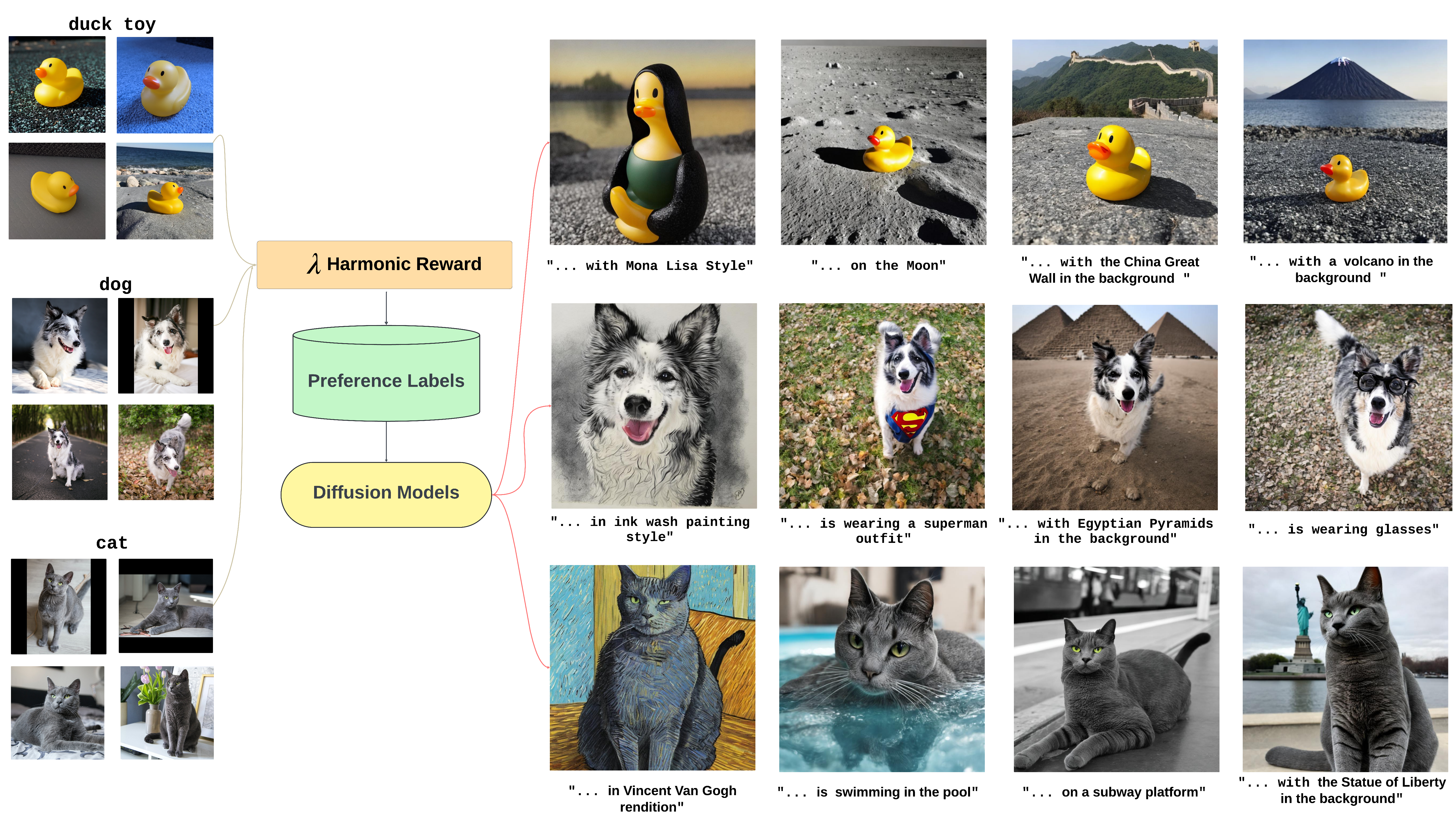
In this paper, we propose a -Harmonic reward function that enables early stopping and accelerate training. In addition, we incorporate the Bradley-Terry preference model to generate preference labels and utilize preference-based reinforcement learning algorithms to finetune pre-trained diffusion models and achieve text-to-image alignment without optimizing any text-encoder or text-embedding. The whole finetuning process including setup, training, validation, and model saving only takes 5 to 20 minutes on Cloud TPU V4. Our method, Reward Preference Optimization (RPO), only requires a few input reference images and the finetuned diffusion model can generate images that preserve the identity of a specific subject and align well with textual prompts (Figure 1).
To show the effectiveness of our -Harmonic reward function, we evaluate RPO on diverse subjects and text prompts on DreamBench [21] and we report the DINO and CLIP-I/CLIP-T of RPO’s generated images on this benchmark and compare them with existing methods. Surprisingly, our method requires a simple setup ( of DreamBooth configuration) and with a small number of gradient steps, but the experimental results outperform or match SOTA.
In summary, our contributions are as follows:
-
•
We introduce the -Harmonic reward function, which permits early-stopping to alleviate overfitting in subject-driven generation tasks and to accelerate the finetuning process.
-
•
By combining the -Harmonic reward function and a preference model, we present RPO, which only require a cheap setup but still can provide high quality results.
-
•
We evaluate RPO and show the effectiveness of the -Harmonic function with diverse subjects and various prompts on DreamBench. We achieve results comparable to SOTA.
2 Related Works
Ruiz et al. [21] formulated a class of problems called subject-driven generation, which refers to preserving the appearance of a subject contextualized in different settings. DreamBooth [21] solves the issue of preserving the subject by binding it in textual space with a unique identifier for the subject in the reference images, and simultaneously generating diverse backgrounds by leveraging prior class-specific information previously learned. A related work that could possibly perform the same task is textual inversion [11]. However, its original objective is to produce a modification of the subject or property marked by a unique token in the text. While it can be used to preserve the subject and change the background or setting, the performance is underwhelming compared to DreamBooth in various metrics [21].
The prevalent issue in DreamBooth and textual inversion is the training times [21, 11] since gradient-based optimization has to be performed on their respective models for each subject. Subject-driven text-to-image generator (SuTI) by [7] aims to alleviate this issue by employing apprenticeship learning. By scraping millions of images online, many expert models are trained for each cluster which allows the apprentice to learn quickly from the experts [7]. However, this is an incredibly intensive task with massive computational overhead during training time.
In the field of natural language processing, direct preference optimization has found great success in large language models (LLM) [19]. By bypassing reinforcement learning from human feedback and directly maximizing likelihoods using preference data, LLMs benefit from more stable training and reduced dependency on an external reward model. Subsequently, this inspired Diffusion-DPO by [27] which applies a similar technique onto the domain of diffusion models. However, this relies on a preference labelled dataset, which can be expensive to collect or not publicly available for legal reasons.
Fortunately, there are reward models that can serve as functional substitutes such as CLIP [17] and ALIGN [13]. ALIGN has a dual encoder architecture that was trained on a large dataset. The encoders can produce text and image embeddings, which allows us to obtain pairwise similarity scores by computing cosine similarity. There are also diffusion modeleling techniques that can leverage reward models. An example is denoising diffusion policy optimization (DDPO) by Black et al. [3] that uses a policy gradient reinforcement learning method to encourage generations that leads to higher rewards.
3 Preliminary
In this section, we introduce notations and some key concepts about text-to-image diffusion models and reinforcement learning.
Text-to-Image Diffusion Models.
Diffusion models [12, 23, 25, 26, 24] are a family of latent variable models of the form , where the are noised latent variables of the same dimensionality as the input data . The diffusion or forward process is often a Markov chain that gradually adds Gaussian noise to the input data and each intermediate sample can be written as
| (1) |
where refers to the variance schedule and . Given a conditioning tensor , the core premise of text-to-image diffusion models is to use a neural network that iteratively refines the current noised sample to obtain the previous step sample , This network can be trained by optimizing a simple denoising objective function, which is the time coefficient weighted mean squared error:
| (2) |
where is uniformly sampled from and can be simplified as 1 according to [12, 24, 20].
Reinforcement Learning and Diffusion DPO
Reinforcement Learning for diffusion models [3, 10, 27] aims to solve the following optimization problem:
| (3) |
where is a hyperparameter controlling the KL-divergence between the finetune model and the pre-trained base model . In Equation (14) from Diffusion-DPO [27], the optimal can be approximated by minimizing the negative log-likelihood:
| (4) |
where represents the preference trajectory, i.e., , and and are independent samples from a Gaussian distribution. A detailed description is given in Appendix A.1.
Additional notations.
We use and to represent the reference image and generated image, respectively. denotes the set of reference images, and is the set of generated images. represents the probability that is more preferred than .
4 Method
We present our -Harmonic reward function that provides reward signals for subject-driven tasks to reduce the learned model to be overfitted to the reference images. Based on this reward function, we use Bradley-Terry model to sample preference labels and a preference algorithm to finetune the diffusion model by optimizing both the similarity loss and the preference loss.
4.1 Reward Preference Optimization
In contrast to other fine-tuning applications [27, 16, 19, 18], there is no human feedback in the subject-driven text-to-image generation task. The model only receives a few reference images and a prompt with a specific subject. Hence, we first propose the -Harmonic reward function that can leverage the ALIGN model [13] to provide valid feedback based on the generated image fidelity: similarity to the given reference images and faithfulness to the text prompts.
-Harmonic Reward Function.
The normalized ALIGN-I and ALIGN-T scores can be denoted as
where is the image feature extractor and is the text encoder in the ALIGN model. Given a reference image set , the -Harmonic reward function can be defined by a weighted harmonic mean of the ALIGN-I and ALIGN-T scores,
| (5) |
Compared to the arithmetic mean, there are two advantages to using the harmonic mean: (1) according to AM-GM-HM inequalities [9], the harmonic mean is a lower bound of the arithmetic mean and maximizing this “pessimistic” reward can also improve the arithmetic mean of ALIGN-I and ALIGN-T scores; (2) the harmonic mean is more sensitive to the smaller of the two scores, i.e., a larger reward is only achieved when both scores are relatively large.
For a simple example, consider . If there are two images, and , where the first image achieves an ALIGN-I score of 0.9 and an ALIGN-T score of 0.01, and the second image receives an ALIGN-I score of 0.7 and an ALIGN-T score of 0.21, we may prefer the second image because it has high similarity to the reference images and is faithful to the text prompts. However, using the arithmetic mean would assign both images the same reward of 0.455. In contrast, the harmonic mean would assign the first image a reward of 0.020 and the second image a reward of 0.323, aligning with our preferences. During training, we set , which means the reward model will focus solely on text-to-image alignment because the objective function consists only of a loss for image-to-image alignment. Note that we set to a different value for validation, which evaluates the fidelity of the subject and faithfulness of the prompt. Details can be found in Section 5.
Dataset.
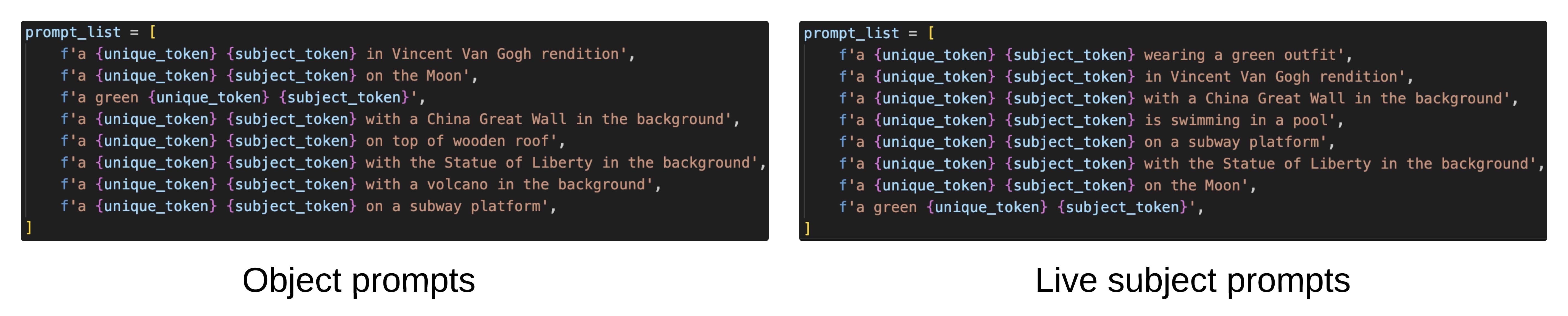
The set of images for subject-driven generative tasks can usually be represented as , where is the image set generated by the base model. DreamBooth [21] requires two different prompts, and , for each subject during the training phase. For example, is ‘‘a photo of [V] dog’’ and is ‘‘a photo of dog’’, where ‘‘[V]’’ is a unique token to specify the subject. DreamBooth then uses to generate for prior preservation loss. Typically, the size of the set of generated images is around 1000, i.e., , which is time-consuming and space-intensive in real applications. However, the diffusion model can only maximize the similarity score and still receives a high reward based on this uninformative prompt . Our method aims to balance the trade-off between similarity and faithfulness. Thus, for efficiency, we introduce 8 novel training prompts, , which can be pre-specified or generated by other Large Language Models111SuTI [7] utilizes PaLM [8] to generate unseen prompts during training. These training prompts include artistic style transfer, re-contextualization, and accessorization. The full list of training prompts is provided in the supplementary material. For example, can be ‘‘a [V] dog is on the Moon’’. We feed these training prompts to the base model and generate 4 images for each training prompt, i.e., .
Once we obtain reward signals, we adopt the Bradley-Terry model [4] to generate preference labels. In particular, given a tuple , we sample preference labels from the following probability model:
| (6) |
Learning.
The learning objective function consist of two parts — similarity loss and preference loss. The similarity loss is designed to minimize the KL divergence between the distribution of reference images and the learned distribution , which is equivalent to minimizing:
| (7) |
The preference loss aims to capture the preference signals and fit the preference model, Eq. (6). Therefore, we use the binary cross-entropy as the objective function for preference loss, combining DPO objective function Eq. 3 the loss function can be written as the following function:
| (8) |
where
and and Combining these two loss functions together, the objective function for finetuning is written as
| (9) |
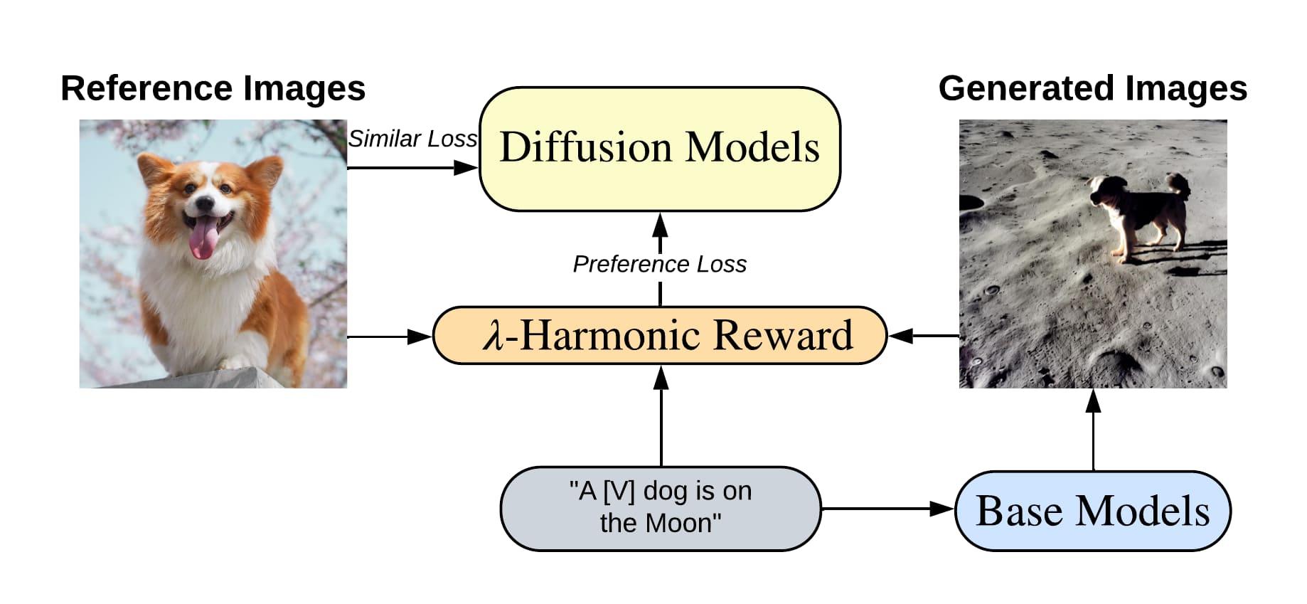
Figure 2 presents an overview of the training method, which includes the base model generated samples, the align reward model, and the preference loss. Note that serves as a regularizer for approximating the text-to-image alignment policy. Conversely, DreamBooth [21] adopts as its regularizer, which cannot guarantee faithfulness to the text-prompt. Based on this loss function and preference model, we only need a few hundred iterations and a small set size of to achieve results that are comparable to, or even better than, the state of the art. The fine-tuning process, which includes generating images, training, and validation, takes about 5 to 20 minutes on a single Google Cloud Platform TPUv4-8 (32GB) for Stable Diffusion.
5 Experiments
In this section, we present the experimental results demonstrated by RPO. We investigate three primary questions. First, can our algorithm learn to generate images that are faithful both to the reference images and to the textual prompts, according to preference labels? Second, if RPO can generate high-quality images, which part is the key component of RPO: the reference loss or the early stopping by the -Harmonic reward function? Third, how do different values affect validation and cause performance differences for RPO? We refer readers to Appendix A.2 for details on the experimental setup, Appendix A.7 for the skill set of RPO, Appendix A.4 for the limitations of the RPO algorithm, and Appendix A.5 for future work involving RPO.
5.1 Dataset and Evaluation
DreamBench.
In this work, we use the DreamBench dataset proposed by DreamBooth [21]. This dataset contains 30 different subject images including backpacks, sneakers, boots, cats, dogs, and toy, etc. DreamBench also provides 25 various prompt templates for each subject and these prompts are requiring the learned models to have such abilities: re-contextualization, accessorization, property modification, and attribute editing.
Evaluation Metrics.
We follow DreamBooth [21] and SuTI [7] to report DINO [5] and CLIP-I [17] for evaluating image-to-image similarity score and CLIP-T [17] for evaluating the text-to-image similarity score. We also use our -Harmonic reward as a evaluation metric for the overall fidelity and the default value of . For evaluation, we follow DreamBooth [21] and SuTI [7] to generate 4 images per prompt, 3000 images in total, which provides robust evaluation.
Baseline algorithms.
DreamBooth [21]: This algorithm requires approximately and 1000 gradient steps to finetune the UNet and text-encoder components. SuTI [7]: A pre-trained method that requires half a million expert models and introduces cross-attention layers into the original diffusion models. Textual Inversion [11]: A text-based method that optimizes the text embedding but freezes the diffusion models. Re-Imagen [6]: An information retrieval-based algorithm that modifies the backbone network architectures and introduces cross-attention layers into the original diffusion models.
5.2 Comparisons
Quantitative Comparisons.
We begin by addressing the first question. We use a quantitative evaluation to compare RPO with other existing methods on three metrics (DINO, CLIP-I, CLIP-T) in DreamBench to validate the effectiveness of RPO. The experimental results on DreamBench is shown in Table 1. We observe that RPO can perform better or on par with SuTI and DreamBooth on all three metrics. Compared to DreamBooth, RPO only requires of the negative samples, but RPO can outperform DreamBooth on the CLIP-I and CLIP-T scores by given the same backbone. Our method outperforms all baseline algorithms in the CLIP-T score, establishing a new SOTA result. This demonstrates that RPO, by solely optimizing UNet through preference labels from the -Harmonic reward function, can generate images that are faithful to the input prompts. Similarly, our CLIP-I score is also the highest, which indicates that RPO can generate images that preserve the subject’s visual features. In terms of the DINO score, our method is almost the same as DreamBooth when using the same backbone. We conjecture that the reason RPO achieves higher CLIP scores and lower DINO score is that the -Harmonic reward function prefers to select images that are semantically similar to the textual prompt, which may result in the loss of some unique features in the pixel space.
| Method | Backbone | Iterations | DINO | CLIP-I | CLIP-T |
|---|---|---|---|---|---|
| Reference Images | N/A | N/A | N/A | ||
| DreamBooth [21] | Imagen [22] | ||||
| DreamBooth [21] | SD [20] | ||||
| Textual inversion [11] | SD [20] | ||||
| SuTI [7] | Imagen [22] | ||||
| Re-Imagen [6] | Imagen [22] | ||||
| Ours: RPO | SD [20] |
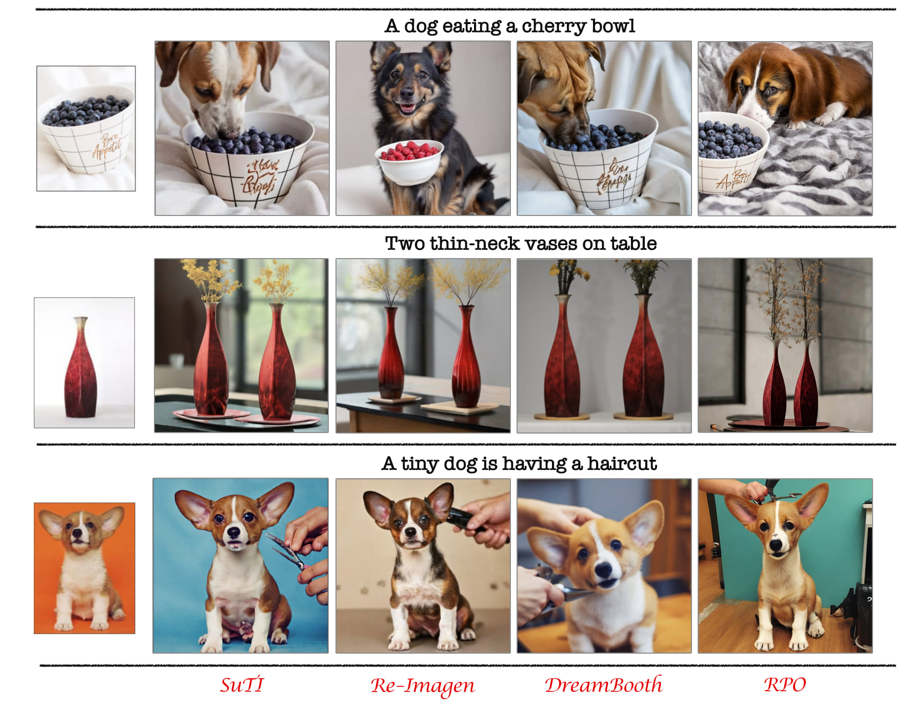
Qualitative Comparisons.
We use the same prompt as SuTI [7], and the generated images are shown in Figure 3. RPO generates images that are faithful to both reference images and textual prompts. We noticed a grammatical mistake in the first prompt used by SuTI [7]; it should be A dog eating a cherry from a bowl. This incorrect prompt caused the RPO-trained model to become confused during the inference phase. However, RPO still preserves the unique appearance of the bowl. For instance, while the text on the bowl is incorrect or blurred in the SuTI and DreamBooth results, RPO accurately retains the words Bon Appetit from the reference bowl images. We also observed that RPO is the only method that generates thin-neck vases. Although existing methods can produce images highly faithful to the reference images, they may not align as well with the textual prompts. We also provide an example in Appendix A.3 that shows how RPO can handle the failure case observed in DreamBooth and SuTI.
| Method | DINO | CLIP-I | CLIP-T | -Harmonic |
|---|---|---|---|---|
| Pure | ||||
| w/o early-stopping | ||||
| Early-stopping w/o | ||||
| RPO () |
| Configuration | DINO | CLIP-I | CLIP-T | -Harmonic |
|---|---|---|---|---|
5.3 Ablation Study and Method Analysis
Preference Loss and -Harmonic Ablation.
We investigate the second primary question through an ablation study. Two regularization components are introduced into RPO: reference loss as a regularizer and early stopping by -Harmonic reward function. Consequently, we compare four methods: (1) Pure , which only minimizes the image-to-image similarity loss ; (2) w/o early stopping, which employs as a regularizer but omits early stopping by -Harmonic reward function; (3) Early stopping w/o , which uses -Harmonic reward function as a regularization method but excludes ; (4) Full RPO, which utilizes both and early stopping by the -Harmonic reward function. We choose the default value in this ablation study.
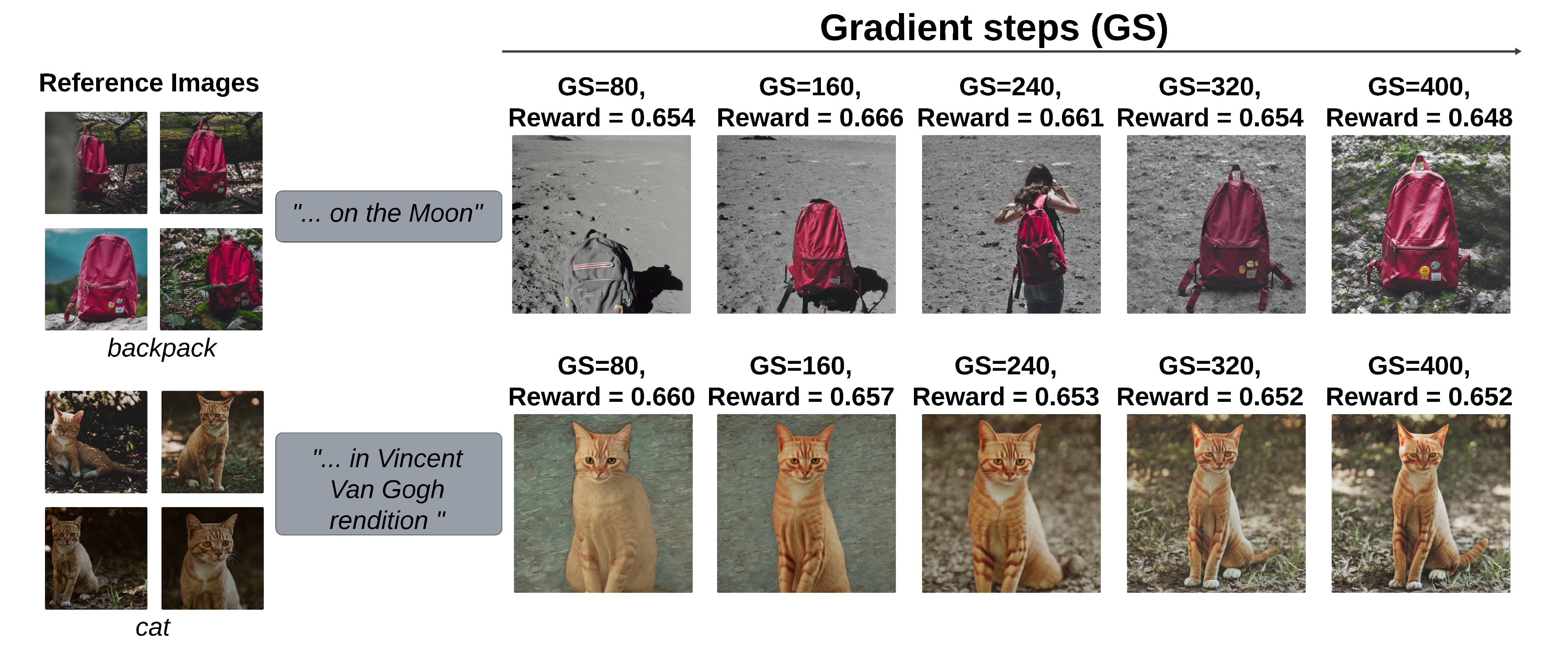
Table 2 lists the evaluation results of these four methods on DreamBench. We observe that without early stopping, can still prevent overfitting to the reference images and improve text-to-image alignment, though the regularization effect is weak. Specifically, the -Harmonic only shows a marginal improvement of 0.003 over pure and 0.001 over early stopping without . The early stopping facilitated by the -Harmonic reward function plays a crucial role in counteracting overfitting, helping the diffusion models retain the ability to generate high-quality images aligned with textual prompts. To provide a deeper understanding of the -Harmonic reward validation, we present two examples from during training in Figure 4, covering both objects and live subjects. We found that the model tends to overfit at a very early stage, i.e., within 200 gradient steps, where -Harmonic can provide correct reward signals for the generated images. For the backpack subject, the generated image receives a low reward at gradient step 80 due to its lack of fidelity to the reference images. However, at gradient step 400, the image is overfitted to the reference images, and the model fails to align well with the input text, resulting in another low reward. -Harmonic assigns a high reward to images that are faithful to both the reference image and textual prompts.
Impact of .
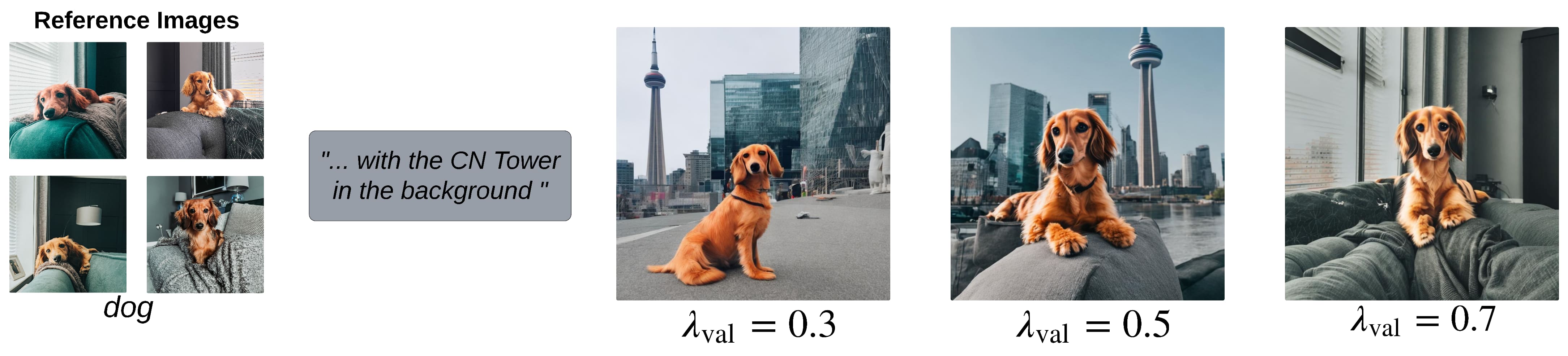
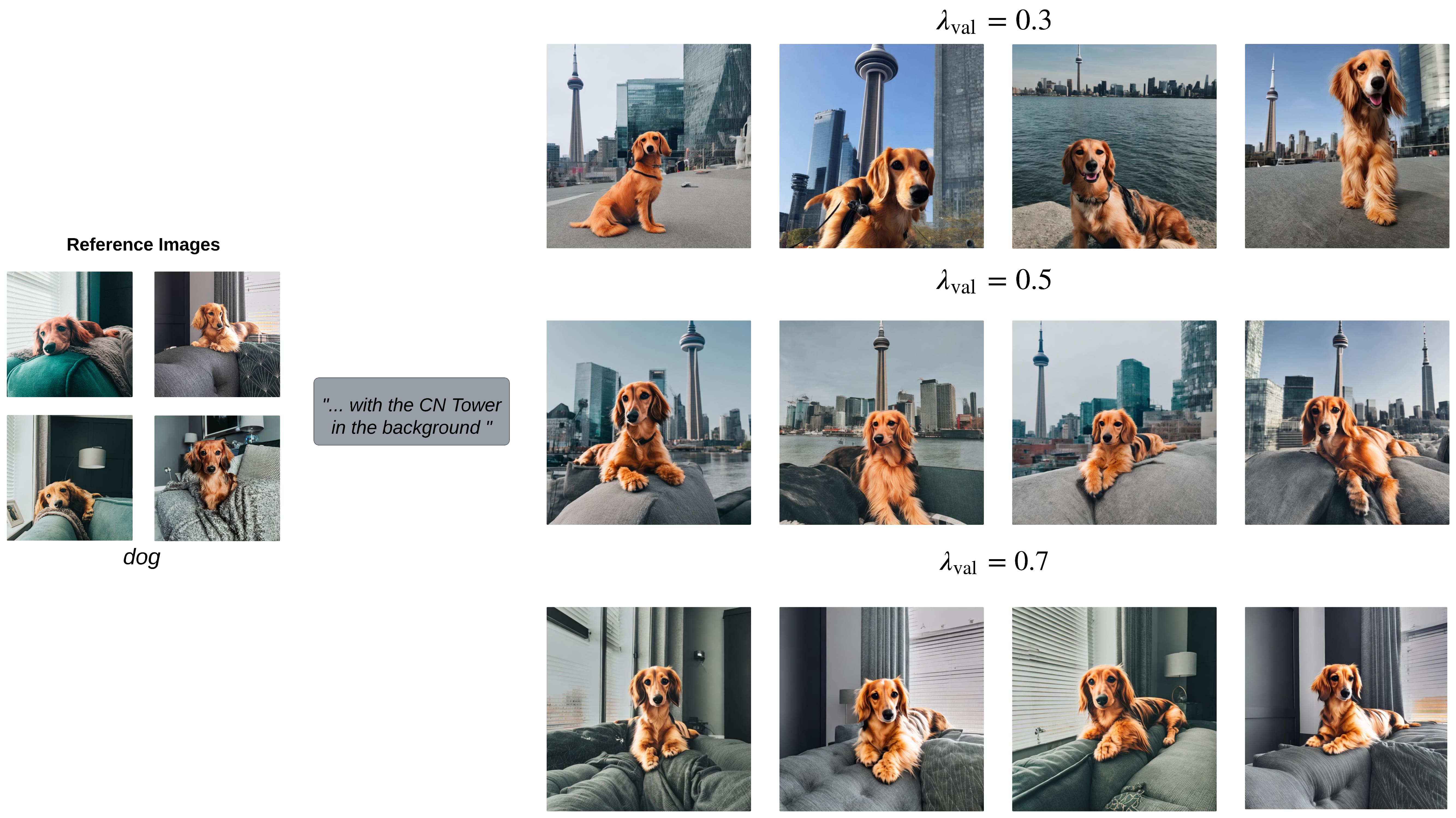
We examine the third primary question by selecting different values from the set as the validation parameters for the -Harmonic reward. According to Equation 5, we believe that as increases, the -Harmonic reward function will give higher weight to the image-to-image similarity score. This will make the generated images more closely resemble the reference images, however, there is also a risk of overfitting. Table 3 shows us the results of three different values on DreamBench. As we expected, a larger makes the images better preserve the characteristics of the reference images, but it also reduces the text-to-image alignment score. Figure 5 shows us an example. In this example, different values lead to different outcomes due to varying strengths of regularization. A smaller can generate more varied results, but seems somewhat off from the reference images. preserves some characteristics beyond the original subject, such as the sofa, but also maintains alignment between text and image. However, when is chosen as an excessively large value, the model actually overfits to the reference images, ignoring the prompts. We have more comparisons in Appendix A.3.
6 Conclusion
We introduce the -Harmonic reward function to derive preference labels and employ RPO to finetune the diffusion model for subject-driven text-to-image generation tasks. Additionally, the -Harmonic reward function serves as a validation method, enabling early stopping to mitigate overfitting to reference images and speeding up the finetuning process.
Acknowledgement
We thank Shixin Luo and Hongliang Fei for providing constructive feedback. This work is supported by a Google grant and with Cloud TPUs from Google’s TPU Research Cloud (TRC).
References
- Bai et al. [2022] Yuntao Bai, Andy Jones, Kamal Ndousse, Amanda Askell, Anna Chen, Nova DasSarma, Dawn Drain, Stanislav Fort, Deep Ganguli, Tom Henighan, et al. Training a helpful and harmless assistant with reinforcement learning from human feedback. arXiv preprint arXiv:2204.05862, 2022.
- Bird et al. [2023] Charlotte Bird, Eddie Ungless, and Atoosa Kasirzadeh. Typology of risks of generative text-to-image models. In Proceedings of the 2023 AAAI/ACM Conference on AI, Ethics, and Society, pages 396–410, 2023.
- Black et al. [2023] Kevin Black, Michael Janner, Yilun Du, Ilya Kostrikov, and Sergey Levine. Training diffusion models with reinforcement learning. arXiv preprint arXiv:2305.13301, 2023.
- Bradley and Terry [1952] Ralph Allan Bradley and Milton E Terry. Rank analysis of incomplete block designs: I. the method of paired comparisons. Biometrika, 39(3/4):324–345, 1952.
- Caron et al. [2021] Mathilde Caron, Hugo Touvron, Ishan Misra, Hervé Jégou, Julien Mairal, Piotr Bojanowski, and Armand Joulin. Emerging properties in self-supervised vision transformers. In Proceedings of the IEEE/CVF international conference on computer vision, pages 9650–9660, 2021.
- Chen et al. [2022] Wenhu Chen, Hexiang Hu, Chitwan Saharia, and William W Cohen. Re-imagen: Retrieval-augmented text-to-image generator. arXiv preprint arXiv:2209.14491, 2022.
- Chen et al. [2024] Wenhu Chen, Hexiang Hu, Yandong Li, Nataniel Ruiz, Xuhui Jia, Ming-Wei Chang, and William W Cohen. Subject-driven text-to-image generation via apprenticeship learning. Advances in Neural Information Processing Systems, 36, 2024.
- Chowdhery et al. [2023] Aakanksha Chowdhery, Sharan Narang, Jacob Devlin, Maarten Bosma, Gaurav Mishra, Adam Roberts, Paul Barham, Hyung Won Chung, Charles Sutton, Sebastian Gehrmann, et al. Palm: Scaling language modeling with pathways. Journal of Machine Learning Research, 24(240):1–113, 2023.
- Djukić et al. [2006] Dušan Djukić, Vladimir Janković, Ivan Matić, and Nikola Petrović. The IMO compendium: a collection of problems suggested for the International Mathematical Olympiads: 1959-2004, volume 119. Springer, 2006.
- Fan et al. [2023] Ying Fan, Olivia Watkins, Yuqing Du, Hao Liu, Moonkyung Ryu, Craig Boutilier, Pieter Abbeel, Mohammad Ghavamzadeh, Kangwook Lee, and Kimin Lee. Reinforcement learning for fine-tuning text-to-image diffusion models. In Thirty-seventh Conference on Neural Information Processing Systems, 2023. URL https://openreview.net/forum?id=8OTPepXzeh.
- Gal et al. [2022] Rinon Gal, Yuval Alaluf, Yuval Atzmon, Or Patashnik, Amit H Bermano, Gal Chechik, and Daniel Cohen-Or. An image is worth one word: Personalizing text-to-image generation using textual inversion. arXiv preprint arXiv:2208.01618, 2022.
- Ho et al. [2020] Jonathan Ho, Ajay Jain, and Pieter Abbeel. Denoising diffusion probabilistic models. Advances in neural information processing systems, 33:6840–6851, 2020.
- Jia et al. [2021] Chao Jia, Yinfei Yang, Ye Xia, Yi-Ting Chen, Zarana Parekh, Hieu Pham, Quoc Le, Yun-Hsuan Sung, Zhen Li, and Tom Duerig. Scaling up visual and vision-language representation learning with noisy text supervision. In International conference on machine learning, pages 4904–4916. PMLR, 2021.
- Kawar et al. [2023] Bahjat Kawar, Shiran Zada, Oran Lang, Omer Tov, Huiwen Chang, Tali Dekel, Inbar Mosseri, and Michal Irani. Imagic: Text-based real image editing with diffusion models. In Proceedings of the IEEE/CVF Conference on Computer Vision and Pattern Recognition, pages 6007–6017, 2023.
- Loshchilov and Hutter [2017] Ilya Loshchilov and Frank Hutter. Decoupled weight decay regularization. arXiv preprint arXiv:1711.05101, 2017.
- Ouyang et al. [2022] Long Ouyang, Jeffrey Wu, Xu Jiang, Diogo Almeida, Carroll Wainwright, Pamela Mishkin, Chong Zhang, Sandhini Agarwal, Katarina Slama, Alex Ray, et al. Training language models to follow instructions with human feedback. Advances in neural information processing systems, 35:27730–27744, 2022.
- Radford et al. [2021] Alec Radford, Jong Wook Kim, Chris Hallacy, Aditya Ramesh, Gabriel Goh, Sandhini Agarwal, Girish Sastry, Amanda Askell, Pamela Mishkin, Jack Clark, et al. Learning transferable visual models from natural language supervision. In International conference on machine learning, pages 8748–8763. PMLR, 2021.
- Rafailov et al. [2024a] Rafael Rafailov, Joey Hejna, Ryan Park, and Chelsea Finn. From to : Your language model is secretly a q-function. arXiv preprint arXiv:2404.12358, 2024a.
- Rafailov et al. [2024b] Rafael Rafailov, Archit Sharma, Eric Mitchell, Christopher D Manning, Stefano Ermon, and Chelsea Finn. Direct preference optimization: Your language model is secretly a reward model. Advances in Neural Information Processing Systems, 36, 2024b.
- Rombach et al. [2022] Robin Rombach, Andreas Blattmann, Dominik Lorenz, Patrick Esser, and Björn Ommer. High-resolution image synthesis with latent diffusion models. In Proceedings of the IEEE/CVF conference on computer vision and pattern recognition, pages 10684–10695, 2022.
- Ruiz et al. [2023] Nataniel Ruiz, Yuanzhen Li, Varun Jampani, Yael Pritch, Michael Rubinstein, and Kfir Aberman. Dreambooth: Fine tuning text-to-image diffusion models for subject-driven generation. In Proceedings of the IEEE/CVF Conference on Computer Vision and Pattern Recognition, pages 22500–22510, 2023.
- Saharia et al. [2022] Chitwan Saharia, William Chan, Saurabh Saxena, Lala Li, Jay Whang, Emily L Denton, Kamyar Ghasemipour, Raphael Gontijo Lopes, Burcu Karagol Ayan, Tim Salimans, et al. Photorealistic text-to-image diffusion models with deep language understanding. Advances in neural information processing systems, 35:36479–36494, 2022.
- Sohl-Dickstein et al. [2015] Jascha Sohl-Dickstein, Eric Weiss, Niru Maheswaranathan, and Surya Ganguli. Deep unsupervised learning using nonequilibrium thermodynamics. In International conference on machine learning, pages 2256–2265. PMLR, 2015.
- Song et al. [2021] Jiaming Song, Chenlin Meng, and Stefano Ermon. Denoising diffusion implicit models. In International Conference on Learning Representations, 2021. URL https://openreview.net/forum?id=St1giarCHLP.
- Song and Ermon [2019] Yang Song and Stefano Ermon. Generative modeling by estimating gradients of the data distribution. Advances in neural information processing systems, 32, 2019.
- Song et al. [2020] Yang Song, Jascha Sohl-Dickstein, Diederik P Kingma, Abhishek Kumar, Stefano Ermon, and Ben Poole. Score-based generative modeling through stochastic differential equations. arXiv preprint arXiv:2011.13456, 2020.
- Wallace et al. [2023] Bram Wallace, Meihua Dang, Rafael Rafailov, Linqi Zhou, Aaron Lou, Senthil Purushwalkam, Stefano Ermon, Caiming Xiong, Shafiq Joty, and Nikhil Naik. Diffusion model alignment using direct preference optimization. arXiv preprint arXiv:2311.12908, 2023.
Appendix A Appendix
A.1 Background
Reinforcement Learning.
In Reinforcement Learning (RL), the environment can be formalized as a Markov Decision Process (MDP). An MDP is defined by a tuple , where is the state space, is the action space, is the transition function, is the reward function, is the distribution over initial states, and is the time horizon. At each timestep , the agent observes a state and selects an action according to a policy , and obtains a reward , and then transit to a next state As the agent interacts with the MDP, it produces a sequence of states and actions, which is denoted as a trajectory . The RL objective is to maximize the expected value of cumulative reward over the trajectories sample from its policy:
Diffusion MDP
We formalize the denoising process as the following Diffusion MDP:
where can be a reward signal for the denoised image. The transition kernel is deterministic, i.e., For brevity, the trajectory is defined by Hence, the trajectory distribution for given diffusion models can be denoted as the joint distribution . In particular, the RL objective function for finetuning diffusion models can be re-written as the following optimization problem:
where is a hyperparameter controlling the KL-divergence between the finetune model and the base model . This constraint prevents the learned model from losing generation diversity and falling into ’mode collapse’ due to a single high cumulative reward result. In practice, this KL-divergence has become a standard constraint in large language model finetuning [1, 16, 19].
Given preference labels and following the Direct Preference Optimization (DPO) framework [27, 19, 18], we can approximate the optimal policy by minimizing the upper bound:
where represents the preference trajectory, i.e., , and and are independent samples from Gaussian distribution. The detailed derivation can be found in [27].
A.2 Experimental Details
Training Prompts.
We collect 8 training prompts: 6 re-contextualization, 1 property modification and 1 artistic style transfer for objects. 5 re-contextualization, 1 attribute editing, 1 artistic style transfer and 1 accessorization for live subjects. The trainig prompts are shown in Figure 6
Experimental Setup
During training we use for the -Harmonic reward function to generate the preference labels. We evaluate the model performance by -Harmonic per 40 gradient steps during training time and save the checkpoint that achieve the highest validation reward. Table 4 lists the common hyperparameters used in the generating skill set and the used in the default setting.
| Parameter | Value |
| Optimization | |
| optimizer | AdamW [15] |
| learning rate | |
| weight decay | |
| gradient clip norm | |
| RPO | |
| regularizer weight, | |
| gradient steps | |
| training preference weight, | |
| validation preference weight (default), |
A.3 Additional Comparisons
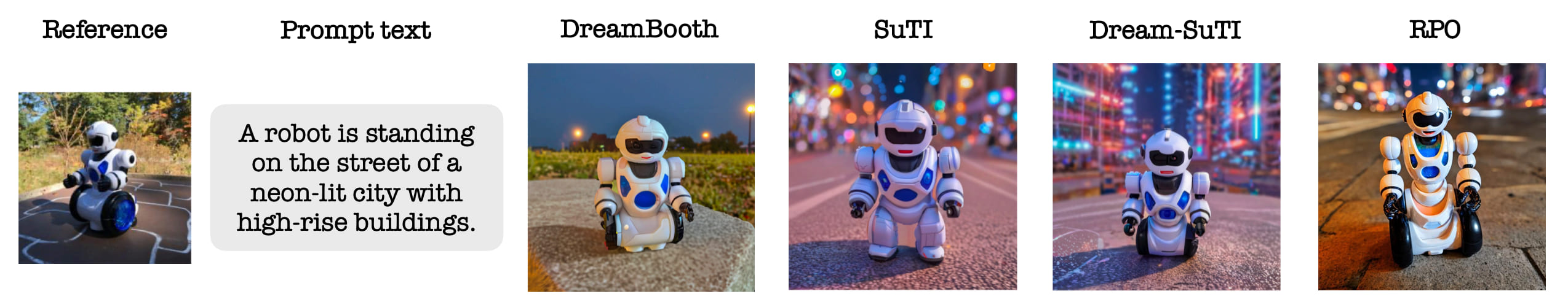
We observe RPO that can be faithful to both reference images and the input prompt. To investigate whether RPO can provide better quality than DreamBooth and SuTI, we follow SuTI paper and pick the robot toy as an example to demonstrate the effectiveness of RPO (Figure 7). In this example, DreamBooth is faithful to the reference image but it does not provide a good text-to-image alignment. SuTI provides an result that is fidelty to textual prompt. However, SuTI lacks fidelity to the reference image, i.e., the robot should stand with its wheels instead of legs. [7] use DreamBooth to finetune SuTI (Dream-SuTI) further to solve this failure case. Instead, RPO can generate an image not only faithful to the reference images but also align well with the input prompts.
We have also added more samples for comparison of different values (see Figure 8). We find that encourages the learned model to retain output diversity while still aligning with textual prompts. However, the generated images invariably contain a sofa, which is unrelated to the subject images. This occurs because every training image includes a sofa. A large weakens the regularization strength and leads to overfitting. Nevertheless, a small value of can potentially eliminate background bias. We highlight that this small not only encourages diversity but also mitigates background bias in identity preservation and enables the model to focus on the subject.
A.4 Limitations
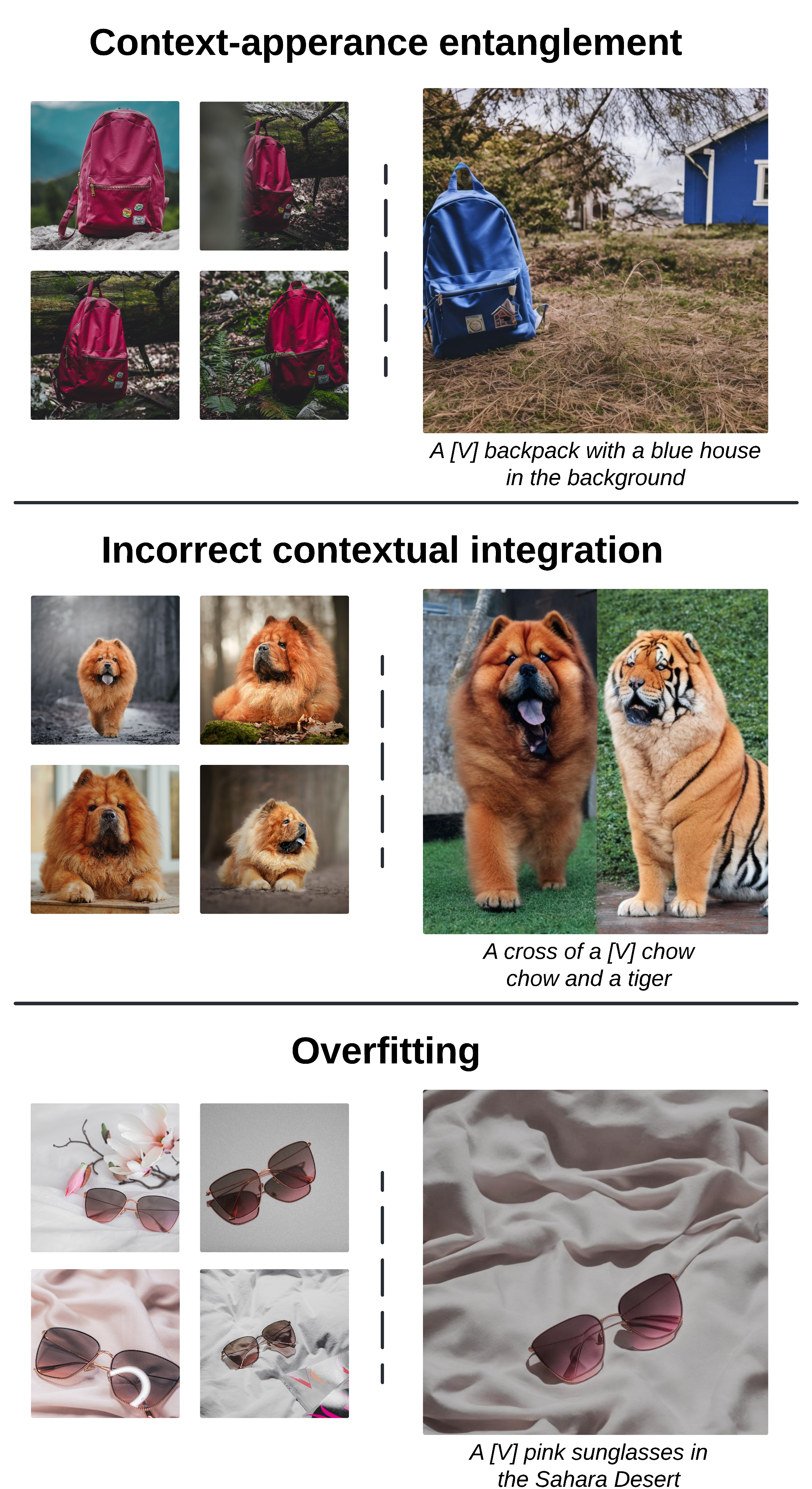
Figure 9 illustrates some failure examples of RPO. The first issue is context-appearance entanglement. In Figure 9, the learned model correctly understands the keyword blue house; however, the appearance of the subject is also altered by this context, e.g. the color of the backpack has changed, and there is a house pattern on the backpack. The second issue is incorrect contextual integration. We conjecture that this failure is due to the rarity of the textual prompt. For instance, imagining a cross between a chow chow and a tiger is challenging, even for humans. Third, although RPO provides regularization, it still cannot guarantee the avoidance of overfitting. As shown in Figure 9, this may be because, to some extent, the visual appearance of sand and bed sheets is similar, which has led to overfitting issues in the model.
A.5 Future Work
The overfitting failure case leads to a future work direction: can online RL improve regularization and avoid overfitting? The second direction for future work involves implementing the LoRA version for RPO and comparing it to LoRA DreamBooth. Last but not least, we aim to identify or construct open-source, subject-driven datasets for comparison. Currently, DreamBench is the only open-source dataset we can access and evaluate for model performance. Nevertheless, we should create a larger dataset that includes more diverse subjects to verify the effectiveness of different algorithms.
A.6 Broader Impacts
The nature of generative image models is inherently subjected to criticism on the issue of privacy, security and ethics in the presence of nefarious actors. However, the core of this paper remains purely on an academic mission to extend the boundaries of generative models. The societal consequences of democratizing such powerful generative models is more thoroughly discussed in other papers. For example, Bird et al. outlines the classes of risks in text-to-image models [2] in greater detail and should be directed to such papers. Nevertheless, we play our part in the management of such risks by avoiding the use of identifiable parts of humans in the reference sets.
A.7 Skill Set
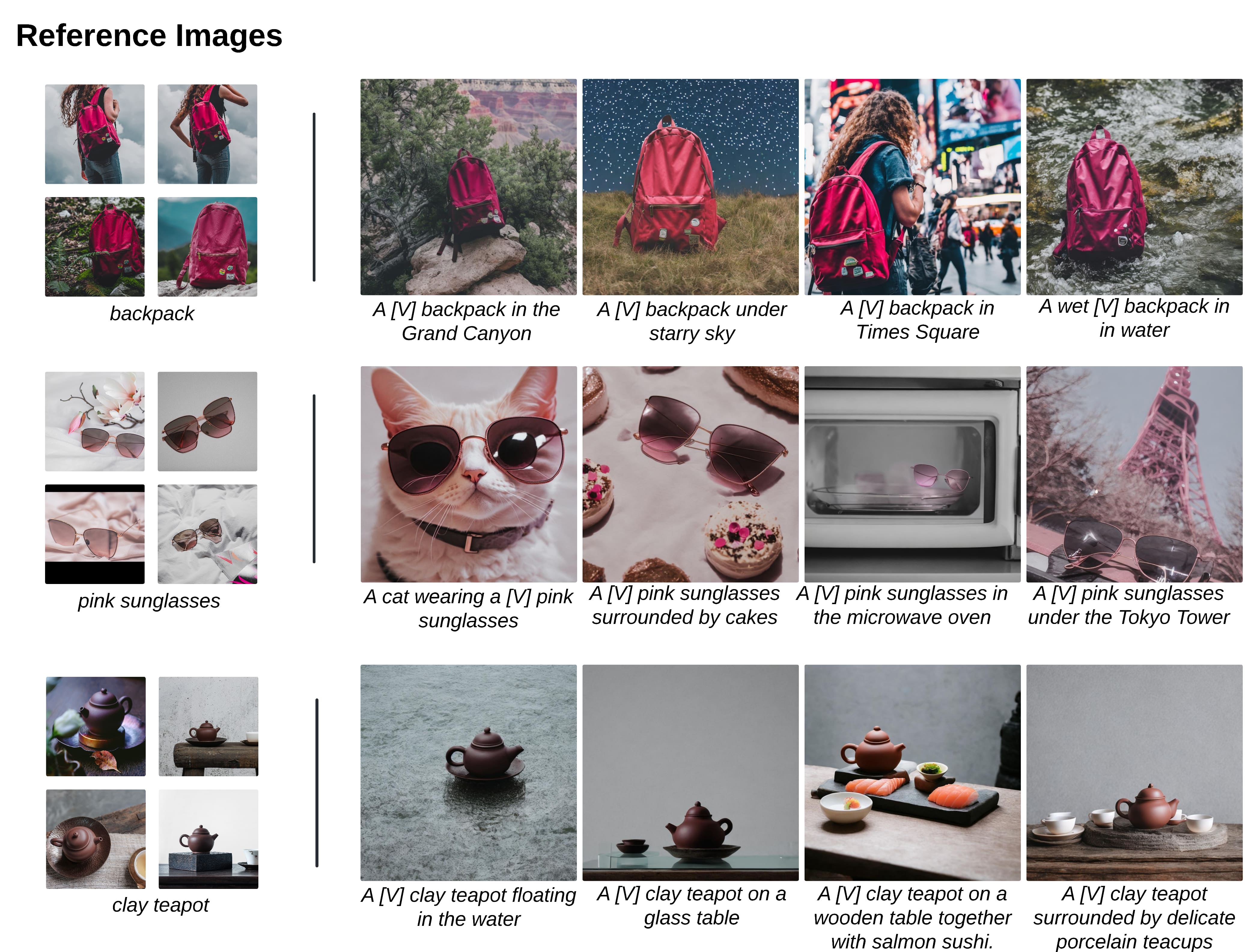
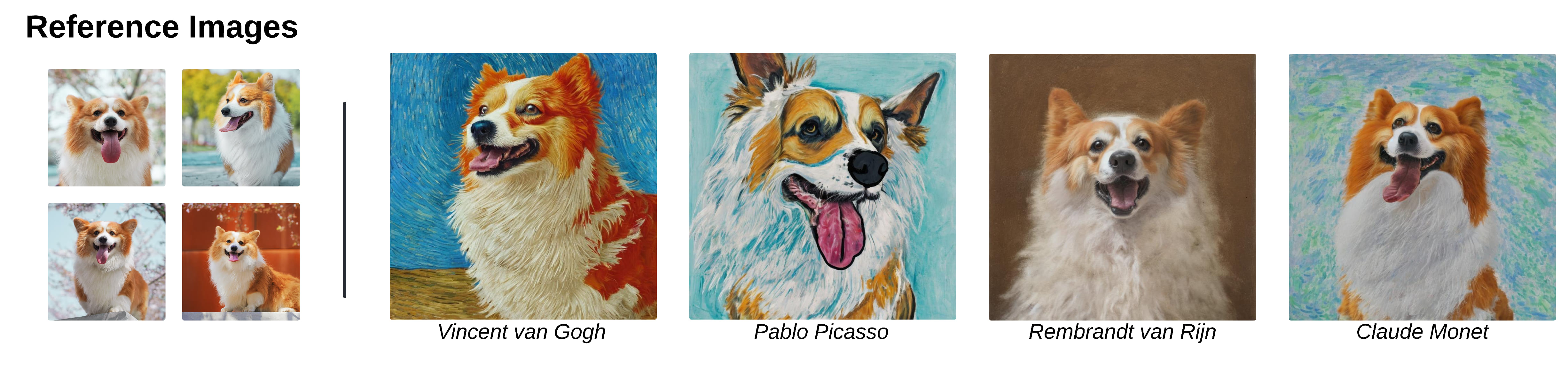
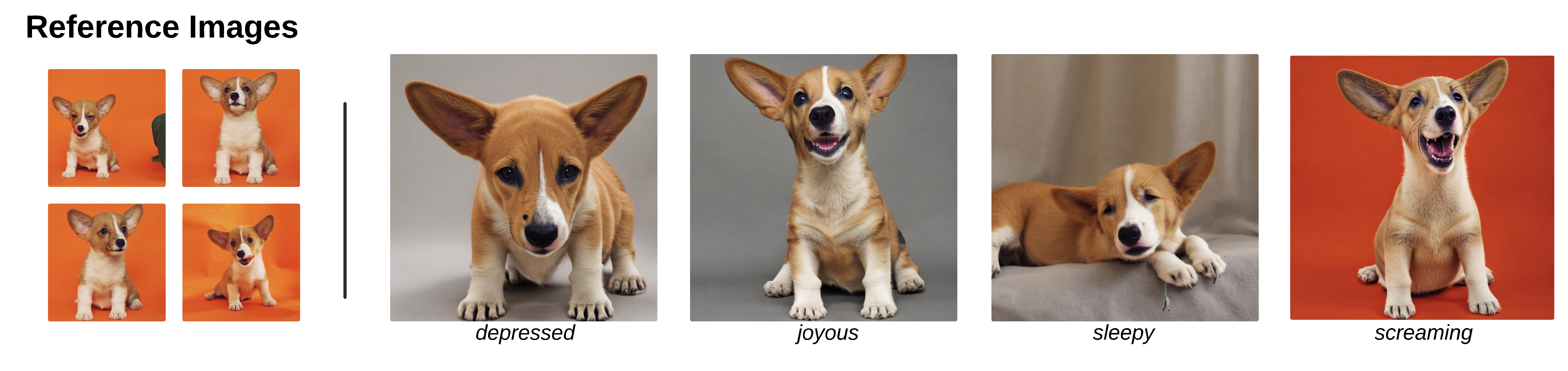
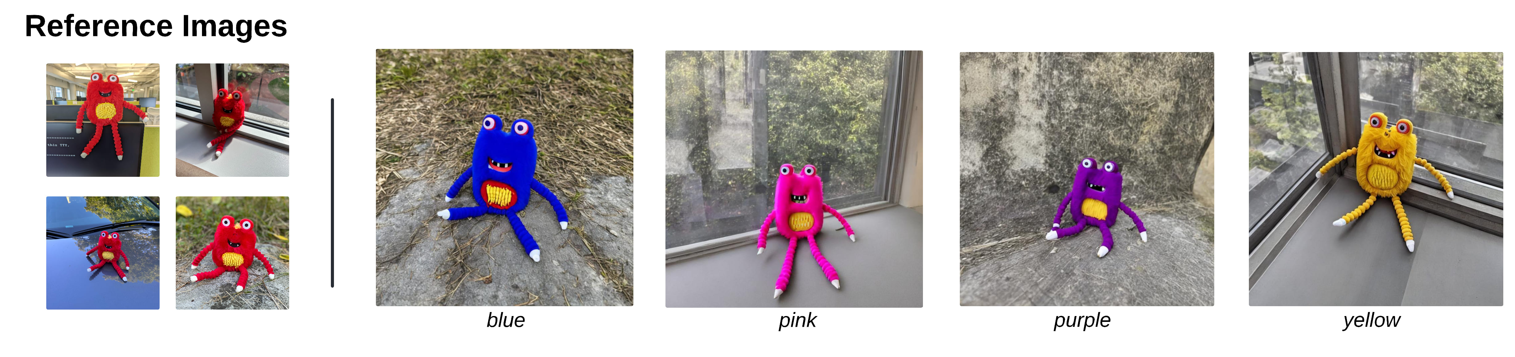
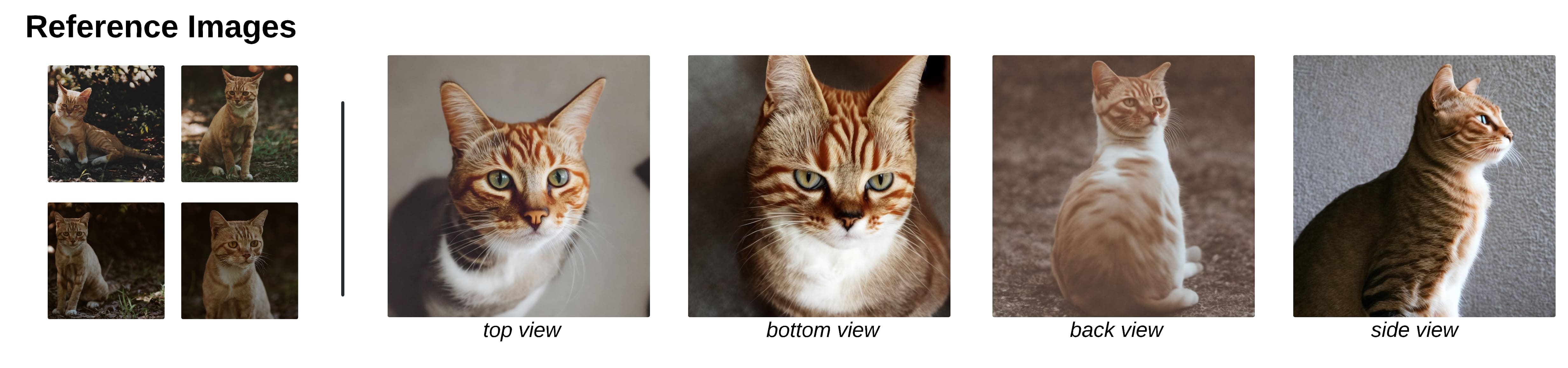
The skill set of the RPO-trained model is varied and includes re-contextualization (Figure 10), artistic style generation (Figure 11), expression modification (Figure 12), subject accessorization (Figure 13), color editing (Figure 14), multi-view rendering (Figure 15), and novel hybrid synthesis (Figure 16).