Revisiting Einstein-Gauss-Bonnet Theories after GW170817
Abstract
In this work we study the inflationary framework of Einstein-Gauss-Bonnet theories which produce a primordial gravitational wave speed that respects the constraint imposed by the GW170817 event, namely in natural units. For these theories in general, the scalar Gauss-Bonnet coupling function is arbitrary and unrelated to the scalar potential. We develop the inflationary formalism of this theory, and present analytic forms for the slow-roll indices, the observational indices and the -foldings number, assuming solely a slow-roll era and also that the constraints imposed by the GW170817 event hold true. We present in detail an interesting class of models that produces a viable inflationary era. Finally, we investigate the behavior of the Einstein-Gauss-Bonnet coupling function during the reheating era, in which case the evolution of the Hubble rate satisfies a constant-roll-like relation . As we show, the behavior of the scalar Gauss-Bonnet coupling during the reheating is different from that of the inflationary era. This is due to the fact that the evolution governing the reheating is different compared to the inflationary era.
pacs:
04.50.Kd, 95.36.+x, 98.80.-k, 98.80.Cq,11.25.-wI Introduction
The inflationary paradigm inflation1 ; inflation2 ; inflation3 ; inflation4 for the early Universe evolution is one exceptional theoretical prediction which explains most of the shortcomings of the Big Bang paradigm and also predicts how the large scale structure of our Universe emerged from the primordial curvature perturbations. To date no sign of inflation has been detected though, and it is vital for the validity of the theory to be observationally confirmed. The next decade is expected to answer the question whether the inflationary era occurred or not, or at least further constrain inflationary theories and give signs or hints that inflation occurred. Indeed, the stage four cosmic microwave background (CMB) experiments that are expected to commence in 2027 CMB-S4:2016ple ; SimonsObservatory:2019qwx , will directly probe the -modes in the CMB polarization pattern, and the future gravitational wave experiments Hild:2010id ; Baker:2019nia ; Smith:2019wny ; Crowder:2005nr ; Smith:2016jqs ; Seto:2001qf ; Kawamura:2020pcg ; Bull:2018lat ; LISACosmologyWorkingGroup:2022jok will probe inflation indirectly via the stochastic gravitational wave background, which is believed to have been generated during the inflationary era. The recent NANOGrav results NANOGrav:2023gor have imposed stringent bounds and constraints on the inflationary era, and it seems highly unlikely that a standard inflationary era can explain the NANOGrav 2023 stochastic gravitational wave background Vagnozzi:2023lwo , however non-standard inflationary scenarios can potentially predict an enhanced inflationary spectrum, see for example Yi:2023mbm ; Balaji:2023ehk . Thus the future experiments are expected to shed light on the question whether inflation actually occurred or not.
Among the candidate theories that can yield an interesting inflationary era are Einstein-Gauss-Bonnet theories Hwang:2005hb ; Nojiri:2006je ; Cognola:2006sp ; Nojiri:2005vv ; Nojiri:2005jg ; Satoh:2007gn ; Bamba:2014zoa ; Yi:2018gse ; Guo:2009uk ; Guo:2010jr ; Jiang:2013gza ; vandeBruck:2017voa ; Pozdeeva:2020apf ; Vernov:2021hxo ; Pozdeeva:2021iwc ; Fomin:2020hfh ; DeLaurentis:2015fea ; Chervon:2019sey ; Nozari:2017rta ; Odintsov:2018zhw ; Kawai:1998ab ; Yi:2018dhl ; vandeBruck:2016xvt ; Maeda:2011zn ; Ai:2020peo ; Easther:1996yd ; Codello:2015mba , which can predict a blue-tilted tensor spectrum. In general, Einstein-Gauss-Bonnet theories are strongly motivated since these are basically string-corrected scalar field theories. Let us recall that the most general scalar field Lagrangian in four dimensions, that contains two derivatives at most is,
| (1) |
and by evaluating the scalar field at its vacuum configuration, it must be either minimally or conformally coupled. By considering the former case, thus and also in the action (1), the most general quantum corrections containing up to fourth order derivatives, of the local effective action, consistent with diffeomorphism invariance, is Codello:2015mba ,
| (2) | ||||
with the parameters , being appropriate dimensionful constants. In 2017 however, the GW170817 event observed by the LIGO-Virgo collaboration TheLIGOScientific:2017qsa ; Monitor:2017mdv ; GBM:2017lvd ; LIGOScientific:2019vic altered our perspective on several candidate theories of inflation, because the observation indicated that the gravitational waves have a propagation speed that it is almost equal to that of light. This result has put severe constraints on theories that predict a propagation speed of tensor perturbations different from that of light, see Refs. Ezquiaga:2017ekz ; Baker:2017hug ; Creminelli:2017sry ; Sakstein:2017xjx ; Boran:2017rdn . However, the GW170817 event is a late-time event, thus one might claim that the speed of primordial tensor perturbations could be different from that of light primordially. This argument however is not correct because inflation is basically a classical theory corresponding to a four dimensional post-Planck Universe. Thus there is no fundamental reason that could make the graviton to change its on-shell mass during and after the inflationary era. Hence, the rule in massive gravity theories is that the speed of tensor perturbations should be equal to that of light. In a series of articles Oikonomou:2021kql ; Oikonomou:2022xoq ; Odintsov:2020sqy , the requirement that the gravitational wave speed is equal to that of light was modelled by using the constraint in Einstein-Gauss-Bonnet theories. This constraint made the scalar potential and the scalar Gauss-Bonnet coupling to be interdependent. In this work we aim to study the inflationary phenomenology of Einstein-Gauss-Bonnet theories by using the actual phenomenological constraints on the gravitational wave speed imposed by the GW170817 event, which is in natural units. Thus, we shall model inflation in Einstein-Gauss-Bonnet theories without taking the constraint into account. In this way, the scalar Gauss-Bonnet coupling function is free to choose and is not directly related to the potential by some physically motivated constraint. We develop the formalism of Einstein-Gauss-Bonnet inflationary theories and we extract analytic relations for the slow-roll indices and the observational indices of inflation. Among a large variety of models, we present a promising class of potentials and scalar Gauss-Bonnet couplings that yield a viable inflationary phenomenology compatible with the GW170817 constraint. Finally, we consider the behavior of the Einstein-Gauss-Bonnet theory during the reheating era, in which case the Hubble rate and its time derivative satisfy a constant-roll-like relation . In this case, the scalar Gauss-Bonnet coupling function is required to obey a differential equation that relates it directly to the scalar potential. We examine several potentials which yielded a viable inflationary phenomenology and we find the functional form of the scalar Gauss-Bonnet coupling for these potentials, and these are different from the forms of the scalar Gauss-Bonnet couplings during the inflationary era.
This article is organized as follows: In section II we develop the Einstein-Gauss-Bonnet inflation formalism, we extract analytic forms for the slow-roll indices and the observational indices of inflation. We also impose several constraints in order to comply with the GW170817 event. In section III we apply the formalism by using a class of models that yields a viable phenomenology for inflationary theories. We determine the range of values of the free parameters of the theory that produce a viable inflationary phenomenology and at the same time a gravitational wave speed which respects the constraint in natural units. Also, in section III we study the behavior of Einstein-Gauss-Bonnet theories during the reheating era and we extract the functional form of the scalar Gauss-Bonnet coupling during this era, given the scalar potential. Finally, the conclusions appear in the end of this article.
II Essential Features of Einstein-Gauss-Bonnet in View of GW170817 Event
We start our analysis by presenting the essential features of Einstein-Gauss-Bonnet theories in view of the GW170817 event. The gravitational action of Einstein-Gauss-Bonnet theories is,
| (3) |
where denotes as usual the Ricci scalar, where is the reduced Planck mass, and also stands for the Gauss-Bonnet invariant in four dimensions, which in terms of the Ricci scalar, the Ricci tensor and the Riemann tensor reads as follows . We assume that the geometric background is a flat Friedmann-Lemaitre-Robertson-Walker (FLRW) spacetime of the form,
| (4) |
We assume that the scalar field is solely time-dependent, so the variation of the gravitational action (3) with respect to the scalar field and with respect to the metric yields the following field equations,
| (5) |
| (6) |
| (7) |
In order for the inflationary era to occur, a requirement is that , and in addition to that we shall assume that the scalar field slow-rolls its potential during the whole inflationary era, so the following requirements are assumed to hold true,
| (8) |
Einstein-Gauss-Bonnet gravities are known to be plagued with the issue related to the propagation speed of primordial gravitational waves, or equivalently with the propagation speed of the tensor perturbations, which is Hwang:2005hb ,
| (9) |
where the functions , and are equal to , , and also . Now there are two ways to take into account the constraints imposed by the GW170817 event, either by requiring that , hence one gets for all the subsequent eras after inflation, or by imposing direct constraints on the values of the terms entering in the gravitational wave speed (9). The first approach was considered in a series of papers Oikonomou:2021kql ; Oikonomou:2022xoq ; Odintsov:2020sqy so we shall not consider this approach in this paper. Instead, we shall assume that the terms entering in the expression of the gravitational wave speed, are sufficiently small, so that the gravitational wave speed satisfies the constraint imposed by the GW170817 event, which is,
| (10) |
In order to achieve this, we assume that,
| (11) |
and if these constraints are satisfied during the inflationary era, then the gravitational wave speed can be sufficiently small in order to satisfy the constraint (10). Let us highlight an important issue here having to do with the inequalities (11), these are not chosen for the sake of analytic simplicity, but these basically quantify the requirement that . Indeed, by looking at Eq. (9) we can see that the gravitational wave speed deviates from unity once the parameter deviates from zero. This parameter can be small enough if , a case thoroughly analyzed in Refs. [56-58], or if each of the terms and are independently very small. This is exactly what the inequalities presented in Eq. (11) signify. Note that the approach we adopted does not constrain the functional form of the Gauss-Bonnet scalar coupling function , which is free to choose, in contrast to the approach adopted in Refs. Oikonomou:2021kql ; Oikonomou:2022xoq ; Odintsov:2020sqy , which constrain the functional form of the Gauss-Bonnet scalar coupling function to be related to the scalar potential. In our approach both the scalar potential and the Gauss-Bonnet scalar coupling function are free to choose. Now let us consider the Friedmann equation, and notice that since we assumed that the constraints of Eq. (11) hold true, the term dominates over the terms . We also make another crucial assumption, regarding the Raychaudhuri equation, that is, we assume that and , that is,
| (12) |
The constraints (12) are additional constraints, which must be satisfied from any viable model. To sum up, the slow-roll and inflationary constraints (8) are natural constraints imposed by inflationary dynamics, the constraints (11) are additional constraints imposed by the GW170817 event, and finally the constraints (12) are rather logical assumptions, which however must be checked if they hold true for any viable model we shall develop. Now in view of the above, the field equations take the simpler form, regarding the Friedmann equation, it becomes,
| (13) |
while the Raychaudhuri equation becomes,
| (14) |
and the modified Klein-Gordon equation yields,
| (15) |
Now the inflationary phenomenology can be studied by using the slow-roll indices and the corresponding observational indices of inflation. Regarding the slow-roll indices, these have the following general form Hwang:2005hb ,
| (16) |
where , , , , , , and also . Regarding the observables of inflation, the scalar spectral index of the primordial curvature perturbations in terms of the slow-roll indices, is equal to,
| (17) |
and the tensor-to-scalar ratio is equal to,
| (18) |
with being the sound speed of the scalar perturbations which is,
| (19) |
and in addition is the gravitational wave speed appearing in Eq. (9). Furthermore, the spectral index of the tensor perturbations is,
| (20) |
An essential and important quantity for the study of the phenomenological viability of an Einstein-Gauss-Bonnet model is the -foldings number expressed in terms of known or given quantities. This is defined as follows,
| (21) |
where and denote the scalar field values at first horizon crossing, in the beginning of inflation, and the end of the inflationary era respectively. We can find the value of the scalar field at the end of inflation easily by equating the first slow-roll index to unity , since the condition indicates the end of inflation, it is the condition of non-acceleration. Alternatively, if the first slow-roll index is constant, another condition would be because this would indicate the end of the slow-roll era, which is equivalent to the end of inflation condition. In view of Eqs. (21) and (15), the -foldings number (21) is written as follows,
| (22) |
which in view of the Friedmann equation (13) is finally written as follows,
| (23) |
Another important quantity, necessary for the phenomenological viability of a model, is the amplitude of scalar perturbations and the constraints on this quantity imposed by the latest Planck data Planck:2018jri . The amplitude of the scalar perturbations is defined as follows,
| (24) |
evaluated at the first horizon crossing when inflation commenced, where is the CMB pivot scale. The constraint on the amplitude of the scalar perturbations coming from the Planck data is Planck:2018jri at the CMB pivot scale. We can express the amplitude of the scalar perturbations in terms of the two point function of the curvature perturbation as follows,
| (25) |
For Einstein-Gauss-Bonnet theories, the amplitude of the scalar perturbations expressed in terms of the slow-roll parameters is given below Hwang:2005hb ,
| (26) |
where and all the quantities must be evaluated at the first horizon crossing, and furthermore at first horizon crossing Hwang:2005hb .
Now, we have all the necessary formulas in order to perform viable model building for GW170817-compatible Einstein-Gauss-Bonnet theories, so let us recapitulate here all the necessary formulas and techniques, and also we discuss the strategy towards choosing a convenient form for the Gauss-Bonnet scalar coupling function. One starts by solving the equation , and the value of the scalar field is determined. Then one solves the equation (22) with respect to , after the integration is performed, and accordingly the slow-roll indices and the observational indices of inflation are evaluated for the value of the scalar field at first horizon crossing.
Regarding the strategy we shall adopt for choosing the appropriate functional form for the Gauss-Bonnet coupling function , the choice will be made based on which one yields analytically simple results. In the present formalism is basically free to choose and it is not constrained in any way, in contrast to the scenario studied in Refs. Oikonomou:2021kql ; Oikonomou:2022xoq ; Odintsov:2020sqy . Thus in the case at hand, the most elegant solution and simple to extract will be determined by the functional form of the first slow-roll index and by the integral in Eq. (23). The exact form of the slow-roll index in terms of the scalar potential is very simple, so by using the Friedmann equation (13), the Raychaudhuri equation (14) and the modified Klein-Gordon equation (15), we get,
| (27) |
and the important issue is to find a convenient form for which can simplify both the functional form of appearing in Eq. (27) and also to simplify the quantity appearing in the integral (23). In view of this line of research, in the next section we shall present several classes of models we did examine and we analyze the resulting phenomenology in detail, also examining whether the constraints we assumed hold true.
III Phenomenological Viability of Several Classes of Einstein-Gauss-Bonnet Models
In this section we shall consider several viable models of Einstein-Gauss-Bonnet gravity which yield both a viable inflationary era and also produce a propagation speed of tensor perturbations that is almost equal to the speed of light and satisfy the constraint (10). For convenience, we shall use the Planck units system for which,
Among the numerous choices for the Gauss-Bonnet coupling function which can be made, the most viable scenarios and the most easy to tackle analytically are obtained by using the following choice,
| (28) |
In this case, the propagation speed of the tensor perturbations acquires a simple form, which is,
| (29) |
and the first slow-roll index takes the form,
| (30) |
while the -foldings number integral takes the form,
| (31) |
Also the tensor-to-scalar ratio takes the form,
| (32) |
while the rest of the observational indices and the slow-roll parameters have quite complicated form to present these here. Now, there are many potentials that can generate a viable evolution, which we list here,
| (33) |
| (34) |
| (35) |
| (36) |
From the above, the last one, namely (36) is viable only for a short inflationary era with -foldings, so let us consider three examples from the above which are viable for -foldings and also have some physical significance in single field scalar field theories. Consider first the potential,
| (37) |
which is known in single scalar field theory as radion gauge inflation scalar potential (RGI), developed in Ref. Fairbairn:2003yx . In this case, the analytic form of the derivative of the Gauss-Bonnet scalar coupling function in Planck units is,
| (38) |
hence the first slow-roll index takes the form,
| (39) |
and therefore one may solve the equation and obtain , but we do not quote it here because it is too lengthy. In this case, the integral involved in the computation of the -foldings number is quite easy to obtain, and it is equal to,
| (40) |
and from it, the value of the scalar field at the beginning of inflation, namely can be obtained. A viable phenomenology is obtained for for various choices of the free parameters , for example for , in which case we get, , and , hence the model is viable regarding the observational indices of inflation and well compatible with the Planck data. In Fig. 1 we plot the model’s predictions versus the Planck 2018 likelihood curves, for and it is apparent that the model is viable.
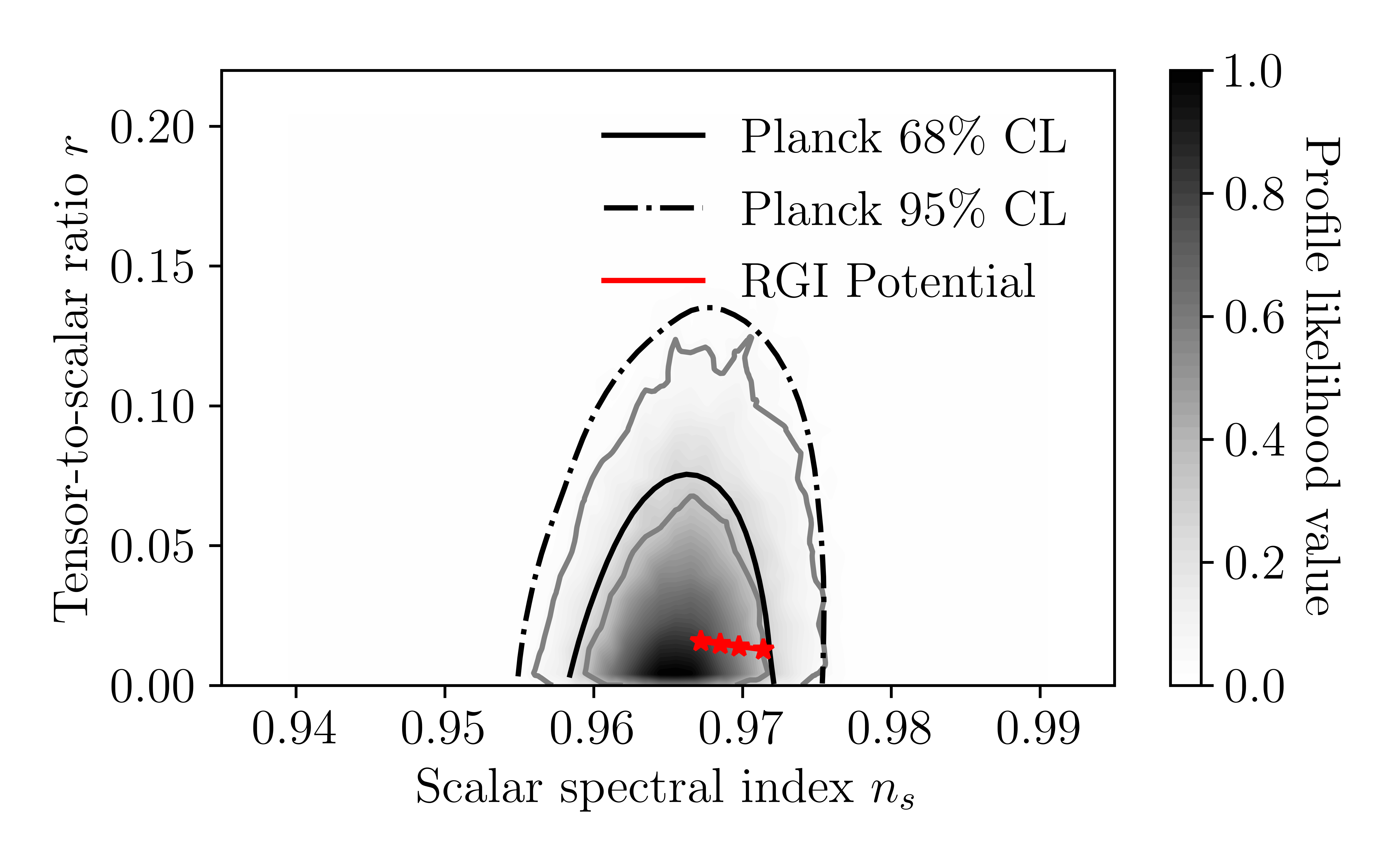
Regarding the amplitude of the scalar perturbations for the current model, for the choice we get exactly , and the amplitude of the scalar perturbations crucially depends on the value of as expected. For we obtain super-Planckian values for the scalar field at the beginning and the end of inflation, but this is a model dependent feature as we show later using other models. For we get, . Regarding the gravitational wave speed, we have , so the model is consistent with the constraint (10). Regarding the constraints (12), these are well satisfied since for we have , and . In Table 1 we collect the characteristic features of this model for convenience.
| Model | Planck Constraints | Values of Scalar Field | Gravitational Wave Speed |
|---|---|---|---|
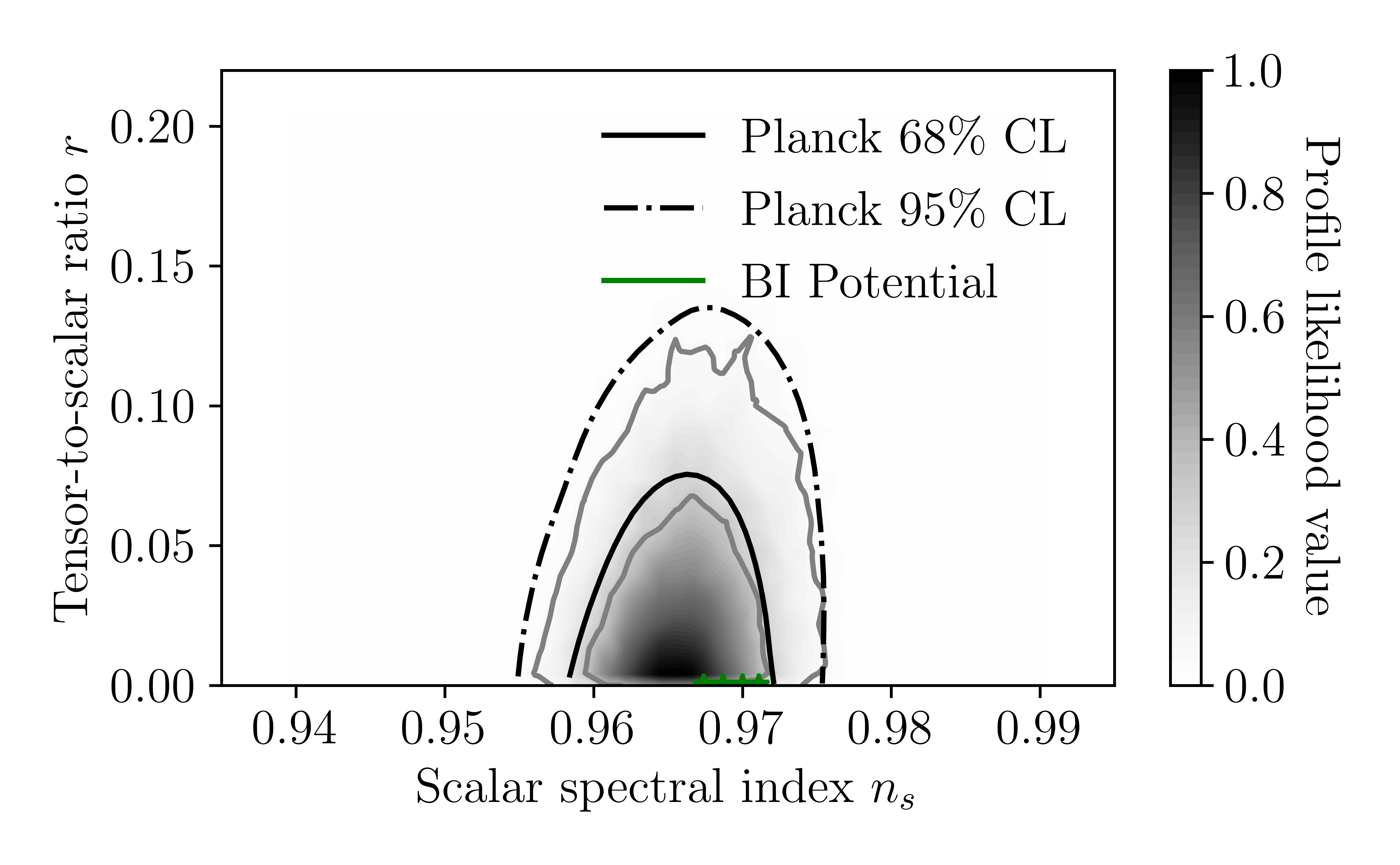
Let us now consider the potential,
| (41) |
which is known in the single scalar field theory literature as brane inflation potential (BI), developed in Refs. Lorenz:2007ze ; Jones:2002cv ; Alexander:2001ks ; Burgess:2001fx ; Pogosian:2003mz ; Brandenberger:2007ca ; Ma:2008rf . In this case, the derivative of the Gauss-Bonnet scalar coupling function in natural units has the form,
| (42) |
and the first slow-roll index becomes,
| (43) |
and therefore one may again solve the equation and obtain the value , which we omit for brevity. In the case at hand, the integral involved in the computation of the -foldings number becomes,
| (44) |
and accordingly, the value of the scalar field can be obtained. In this case too, a large range of the values of the free parameters can guarantee a viable inflationary phenomenology, for example for and for , we get, , and , therefore the model is viable regarding the observational indices of inflation and well compatible with the Planck data. This can also be seen in Fig. 2 where we plot the current model’s predictions versus the Planck 2018 likelihood curves, for .
Regarding the amplitude of the scalar perturbations in this case, for the choice we get exactly , and as expected, the amplitude of the scalar perturbations crucially depends on the value of in this case too. For in this case, the scalar field values at the beginning and the end of inflation are sub-Planckian, specifically, for we get, . Regarding the gravitational wave speed, in this case we have , so in this case too, the model is consistent with the constraint (10). Regarding the constraints (12), these are well satisfied for this model too, for example for we have , and . In Table 1 we collected all the characteristic features for this model too. Let us now consider another viable potential,
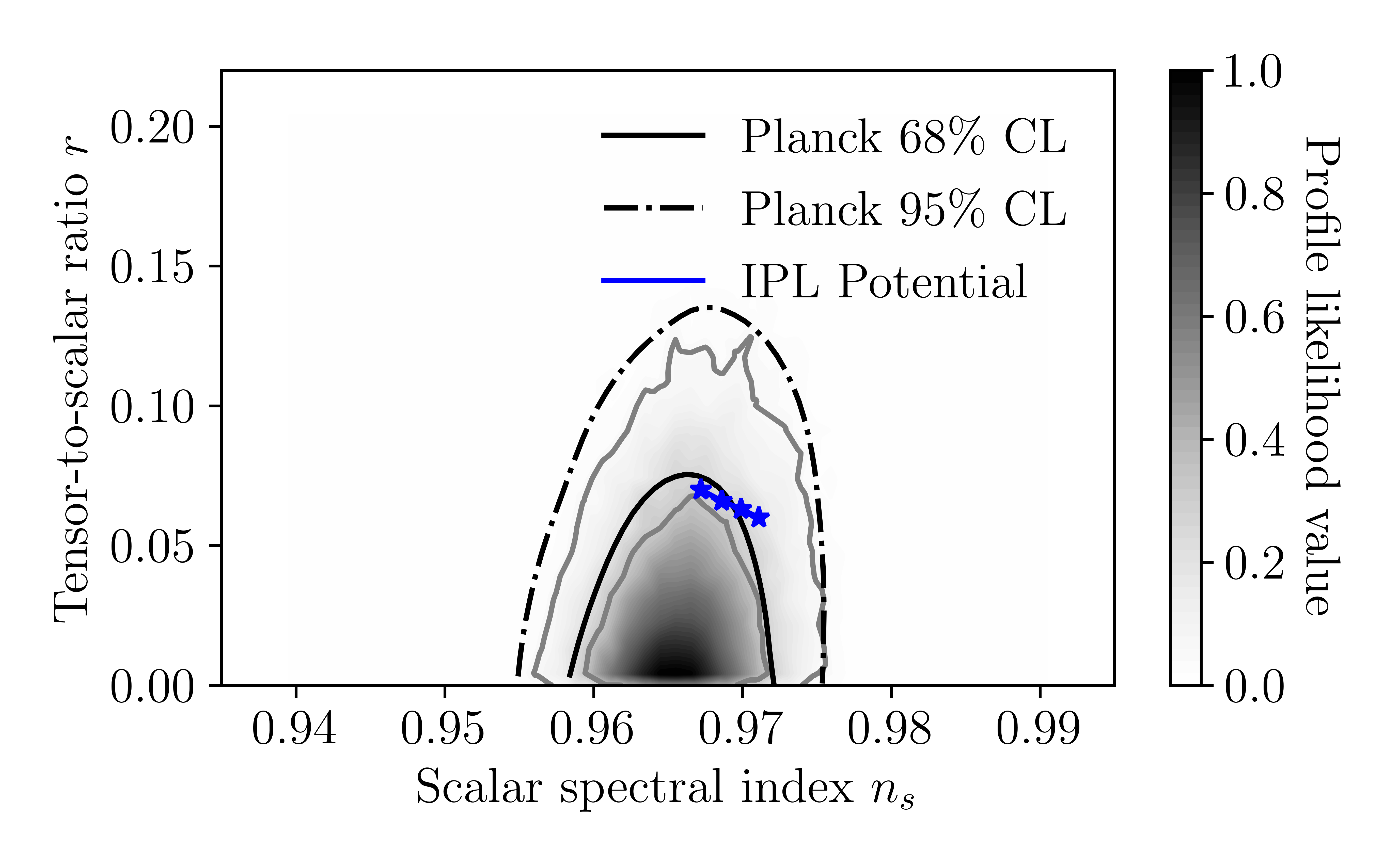
| (45) |
which is not classified into known single scalar field potentials, but provides an interesting viable phenomenology, and we call it inverse power law (IPL). In this case, the derivative of the Gauss-Bonnet scalar coupling function in natural units has the form,
| (46) |
and the first slow-roll index becomes in this case,
| (47) |
and again one may solve the equation and obtain the value , which we again omit for brevity. In this case, the integral involved in the computation of the -foldings number becomes,
| (48) |
and accordingly, the value of the scalar field can be obtained. In this scenario too, a large range of the values of the free parameters guarantees a viable inflationary phenomenology, for example for and if we choose , we get, , and , therefore the model is marginally viable regarding the observational indices of inflation and well compatible with the Planck data. This can also be seen in this case in Fig. 3 where we plot the current model’s predictions versus the Planck 2018 likelihood curves, for .
Now, regarding the amplitude of the scalar perturbations in this case, for the choice we get exactly . For in this case, the scalar field values at the beginning and the end of inflation are super-Planckian, specifically, for we get, , and this is a model dependent feature, in other models we found, the scalar field values are sub-Planckian. In all the cases we found, it is mentionable that the scalar field values decrease as time evolves, which is an anticipated feature, which we shall use in the next section. Regarding the gravitational wave speed, in this case we have , so in this case too, the model is consistent with the constraint (10). Regarding the constraints (12), these are well satisfied for this model too, for example if we choose we get , and . In Table 1 we collected all the characteristic features for this model too.
In conclusion, we presented a variety of models which provide a viable inflationary era, in addition to the compatibility with all the constraints coming from GW170817 and all the additional required constraints. Now in the next section we shall consider an important issue having to do with the functional form of the Gauss-Bonnet coupling function during the reheating era. In this section we chose arbitrarily the scalar Gauss-Bonnet coupling, however this is not the case in the reheating era, in which case the functional form of the scalar Gauss-Bonnet coupling is related to the form of the given potential. An outcome of this section that will be used in the next section, is the well anticipated fact that the scalar field values decrease as the cosmic time evolves.
IV Behavior of the Einstein-Gauss-Bonnet Gravity During the Reheating Era
In this section we shall investigate the reheating era for the Einstein-Gauss-Bonnet gravity framework we developed in the previous sections, and we shall demonstrate that the scalar Gauss-Bonnet coupling is constrained to be related to the scalar potential. The scale factor of the Universe during the reheating era is assumed to have the general form (assuming that ) which results to the relation between the Hubble rate and its time derivative . Now the reason for this is simple, the total equation of state (EoS) parameter , defined as,
| (49) |
during the reheating era takes values in the range , which is explained simply because the value corresponds to the non-acceleration value exactly at the end of the inflationary era, while corresponds to the value of a radiation domination era. The reheating era though is a vague era for which little are known thus it is far from certain what was the total EoS parameter during that era. We will thus assume that during the reheating era, the total EoS parameter takes various characteristic values, varying from the value nearly at the end of the inflationary era, to the value during the radiation domination era . Specifically, we assume that which corresponds to (which is slightly smaller than the end of inflation era value of the EoS ), which corresponds to and describes a matter domination era, and finally which corresponds to and describes a radiation domination era. One can easily work out this scenario to find the behavior of the Gauss-Bonnet scalar coupling function , assuming again that the inequalities of Eq. (11) hold true, so after some algebra one gets,
| (50) |
| (51) |
| (52) |
and finally,
| (53) |
with,
| (54) |
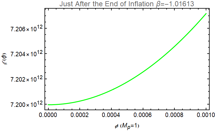
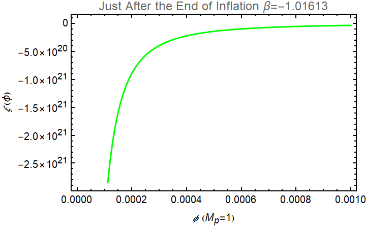
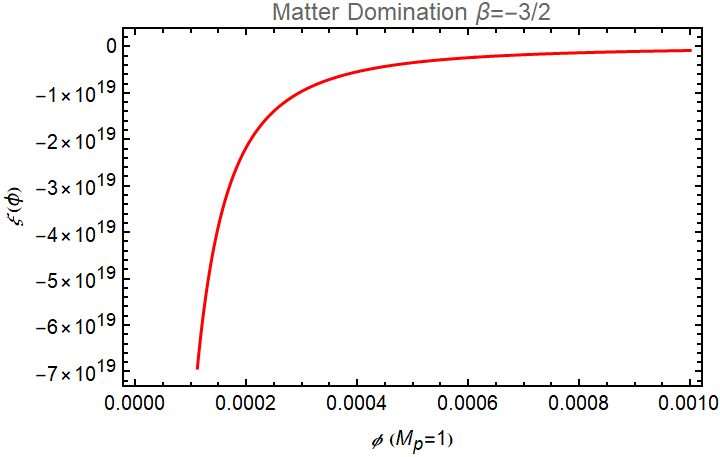
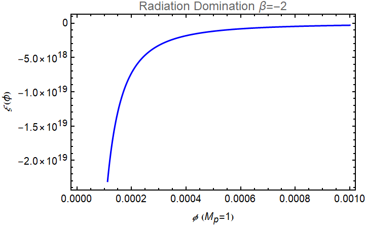
One can solve the differential equation (53), given the scalar field potential, and find the function or can have directly and investigate the behavior of it as a function of the scalar field. We shall reveal the behavior of for the three values of we mentioned earlier and for some characteristic viable potentials we presented in the previous section, using the corresponding values of the free parameters in order to see the behavior of during the reheating era. Consider first the BI potential (41) so by substituting the potential in the differential equation (53) we obtain the following solution for the scalar Gauss-Bonnet coupling function,
| (55) |
Using and working again in Planck units, we can see the behavior of the Gauss-Bonnet coupling function (55) in Fig. 4, for which corresponds to the green curve (nearly the end of inflation era value of the total EoS ), (matter domination era and red curve) and (radiation domination era and blue curve). As it can be seen, as the scalar field values increase, the scalar Gauss-Bonnet scalar coupling decreases, for all the aforementioned cases, the difference is the magnitude of the function for the three distinct scenarios.
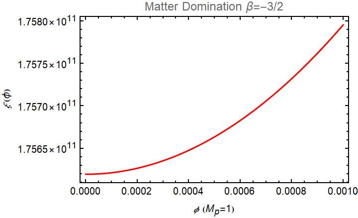
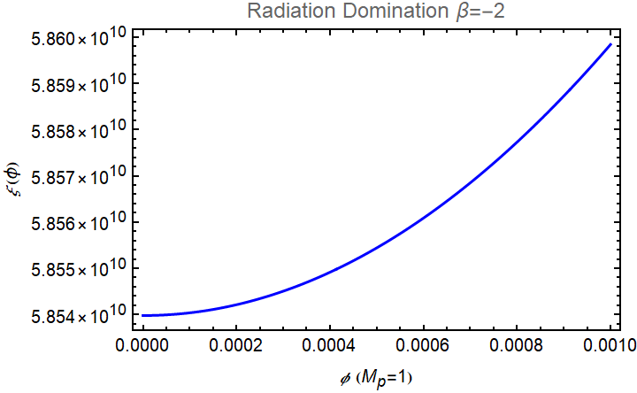
Now let us consider the RDI potential (37) so by substituting the potential in the differential equation (53) in this case we obtain the following solution,
| (56) |
Using in Planck units, we plot the Gauss-Bonnet coupling function (56) as a function of the scalar field in Fig. 5. Contrary to the previous model, in this case the scalar Gauss-Bonnet coupling function increases as the scalar field values increase. The behavior for the three distinct values of we used is qualitatively similar and the only difference among the three cases for the potential under study is, as in the previous case, the magnitude of the Gauss-Bonnet coupling function.
In conclusion, the behavior of the scalar Gauss-Bonnet coupling during the reheating era for the Einstein-Gauss-Bonnet models we considered in this paper strongly depends on the scalar potential. Thus it cannot be predicted how will behave and its behavior is more or less model dependent. Now a crucial comment would be, whether the constrained form of the scalar Gauss-Bonnet coupling function obtained during the reheating, can be the same during the inflationary era. This is hard to decide because this constraint was obtained for a constant-roll-like evolution of the form , and this would imply that the inflationary era would be a power-law evolution. The whole formalism should change though and we did not address this issue in this paper, since it would be out of context. We aim to address this research topic in a future work though.
Concluding Remarks
In this work we developed the inflationary framework of Einstein-Gauss-Bonnet theories that produce a propagating speed of tensor perturbations that respect the constraint imposed by the GW170817 event, namely in natural units. In general, in these theories the scalar Gauss-Bonnet coupling function can be chosen freely and there is no imposed direct relation between the and the scalar potential. We developed the inflationary formalism assuming only a slow-roll era for the scalar field and also imposing the GW170817 constraints on the propagating speed of tensor perturbations which constrain the scalar Gauss-Bonnet coupling function . We applied the formalism using an interesting class of models and for several potentials that produce a viable inflationary era compatible with the Planck constraints and also respect the GW170817 constraints. Also we considered the reheating era in the context of Einstein-Gauss-Bonnet gravitational theories, in which case the Hubble rate obeys a constant-roll-like evolution relation . Assuming that the GW170817 constraints also hold true, it proves that the scalar Gauss-Bonnet coupling function and the scalar potential obey a differential equation. Therefore, given the potential, one finds the scalar Gauss-Bonnet coupling function, which is different from the one during the inflationary era. We considered two examples and we examined the behavior of the scalar Gauss-Bonnet coupling function during the reheating era. An issue which we did not address is to examine the inflationary phenomenology of Einstein-Gauss-Bonnet theories for which the Hubble rate obeys a constant-roll-like evolution during the inflationary era. This would produce a power-law inflationary era, thus the formalism and field equations of the corresponding Einstein-Gauss-Bonnet theory would be different compared to the one we developed here. There is strong motivation for such constant-roll inflationary conditions, which were firstly introduced in Martin:2012pe , for example primordial black hole formation and induced gravitational waves Motohashi:2019rhu ; Tomberg:2023kli . We aim to address this constant-roll inflationary era research task in a future work.
Acknowledgments
This research has been is funded by the Committee of Science of the Ministry of Education and Science of the Republic of Kazakhstan (Grant No. AP14869238).
References
- (1) A. D. Linde, Lect. Notes Phys. 738 (2008) 1 [arXiv:0705.0164 [hep-th]].
- (2) D. S. Gorbunov and V. A. Rubakov, “Introduction to the theory of the early universe: Cosmological perturbations and inflationary theory,” Hackensack, USA: World Scientific (2011) 489 p;
- (3) A. Linde, arXiv:1402.0526 [hep-th];
- (4) D. H. Lyth and A. Riotto, Phys. Rept. 314 (1999) 1 [hep-ph/9807278].
- (5) K. N. Abazajian et al. [CMB-S4], [arXiv:1610.02743 [astro-ph.CO]].
- (6) M. H. Abitbol et al. [Simons Observatory], Bull. Am. Astron. Soc. 51 (2019), 147 [arXiv:1907.08284 [astro-ph.IM]].
- (7) S. Hild, M. Abernathy, F. Acernese, P. Amaro-Seoane, N. Andersson, K. Arun, F. Barone, B. Barr, M. Barsuglia and M. Beker, et al. Class. Quant. Grav. 28 (2011), 094013 doi:10.1088/0264-9381/28/9/094013 [arXiv:1012.0908 [gr-qc]].
- (8) J. Baker, J. Bellovary, P. L. Bender, E. Berti, R. Caldwell, J. Camp, J. W. Conklin, N. Cornish, C. Cutler and R. DeRosa, et al. [arXiv:1907.06482 [astro-ph.IM]].
- (9) T. L. Smith and R. Caldwell, Phys. Rev. D 100 (2019) no.10, 104055 doi:10.1103/PhysRevD.100.104055 [arXiv:1908.00546 [astro-ph.CO]].
- (10) J. Crowder and N. J. Cornish, Phys. Rev. D 72 (2005), 083005 doi:10.1103/PhysRevD.72.083005 [arXiv:gr-qc/0506015 [gr-qc]].
- (11) T. L. Smith and R. Caldwell, Phys. Rev. D 95 (2017) no.4, 044036 doi:10.1103/PhysRevD.95.044036 [arXiv:1609.05901 [gr-qc]].
- (12) N. Seto, S. Kawamura and T. Nakamura, Phys. Rev. Lett. 87 (2001), 221103 doi:10.1103/PhysRevLett.87.221103 [arXiv:astro-ph/0108011 [astro-ph]].
- (13) S. Kawamura, M. Ando, N. Seto, S. Sato, M. Musha, I. Kawano, J. Yokoyama, T. Tanaka, K. Ioka and T. Akutsu, et al. [arXiv:2006.13545 [gr-qc]].
- (14) A. Weltman, P. Bull, S. Camera, K. Kelley, H. Padmanabhan, J. Pritchard, A. Raccanelli, S. Riemer-Sørensen, L. Shao and S. Andrianomena, et al. Publ. Astron. Soc. Austral. 37 (2020), e002 doi:10.1017/pasa.2019.42 [arXiv:1810.02680 [astro-ph.CO]].
- (15) P. Auclair et al. [LISA Cosmology Working Group], [arXiv:2204.05434 [astro-ph.CO]].
- (16) G. Agazie et al. [NANOGrav], Astrophys. J. Lett. 951 (2023) no.1, L8 doi:10.3847/2041-8213/acdac6 [arXiv:2306.16213 [astro-ph.HE]].
- (17) S. Vagnozzi, JHEAp 39 (2023), 81-98 doi:10.1016/j.jheap.2023.07.001 [arXiv:2306.16912 [astro-ph.CO]].
- (18) Z. Yi, Q. Gao, Y. Gong, Y. Wang and F. Zhang, Sci. China Phys. Mech. Astron. 66 (2023) no.12, 120404 doi:10.1007/s11433-023-2266-1 [arXiv:2307.02467 [gr-qc]].
- (19) S. Balaji, G. Domènech and G. Franciolini, JCAP 10 (2023), 041 doi:10.1088/1475-7516/2023/10/041 [arXiv:2307.08552 [gr-qc]].
- (20) J. c. Hwang and H. Noh, Phys. Rev. D 71 (2005) 063536 doi:10.1103/PhysRevD.71.063536 [gr-qc/0412126].
- (21) S. Nojiri, S. D. Odintsov and M. Sami, Phys. Rev. D 74 (2006) 046004 doi:10.1103/PhysRevD.74.046004 [hep-th/0605039].
- (22) G. Cognola, E. Elizalde, S. Nojiri, S. Odintsov and S. Zerbini, Phys. Rev. D 75 (2007) 086002 doi:10.1103/PhysRevD.75.086002 [hep-th/0611198].
- (23) S. Nojiri, S. D. Odintsov and M. Sasaki, Phys. Rev. D 71 (2005) 123509 doi:10.1103/PhysRevD.71.123509 [hep-th/0504052].
- (24) S. Nojiri and S. D. Odintsov, Phys. Lett. B 631 (2005) 1 doi:10.1016/j.physletb.2005.10.010 [hep-th/0508049].
- (25) M. Satoh, S. Kanno and J. Soda, Phys. Rev. D 77 (2008) 023526 doi:10.1103/PhysRevD.77.023526 [arXiv:0706.3585 [astro-ph]].
- (26) K. Bamba, A. N. Makarenko, A. N. Myagky and S. D. Odintsov, JCAP 1504 (2015) 001 doi:10.1088/1475-7516/2015/04/001 [arXiv:1411.3852 [hep-th]].
- (27) Z. Yi, Y. Gong and M. Sabir, Phys. Rev. D 98 (2018) no.8, 083521 doi:10.1103/PhysRevD.98.083521 [arXiv:1804.09116 [gr-qc]].
- (28) Z. K. Guo and D. J. Schwarz, Phys. Rev. D 80 (2009) 063523 doi:10.1103/PhysRevD.80.063523 [arXiv:0907.0427 [hep-th]].
- (29) Z. K. Guo and D. J. Schwarz, Phys. Rev. D 81 (2010) 123520 doi:10.1103/PhysRevD.81.123520 [arXiv:1001.1897 [hep-th]].
- (30) P. X. Jiang, J. W. Hu and Z. K. Guo, Phys. Rev. D 88 (2013) 123508 doi:10.1103/PhysRevD.88.123508 [arXiv:1310.5579 [hep-th]].
- (31) C. van de Bruck, K. Dimopoulos, C. Longden and C. Owen, arXiv:1707.06839 [astro-ph.CO].
- (32) E. O. Pozdeeva, M. R. Gangopadhyay, M. Sami, A. V. Toporensky and S. Y. Vernov, Phys. Rev. D 102 (2020) no.4, 043525 doi:10.1103/PhysRevD.102.043525 [arXiv:2006.08027 [gr-qc]].
- (33) S. Vernov and E. Pozdeeva, Universe 7 (2021) no.5, 149 doi:10.3390/universe7050149 [arXiv:2104.11111 [gr-qc]].
- (34) E. O. Pozdeeva and S. Y. Vernov, Eur. Phys. J. C 81 (2021) no.7, 633 doi:10.1140/epjc/s10052-021-09435-8 [arXiv:2104.04995 [gr-qc]].
- (35) I. Fomin, Eur. Phys. J. C 80 (2020) no.12, 1145 doi:10.1140/epjc/s10052-020-08718-w [arXiv:2004.08065 [gr-qc]].
- (36) M. De Laurentis, M. Paolella and S. Capozziello, Phys. Rev. D 91 (2015) no.8, 083531 doi:10.1103/PhysRevD.91.083531 [arXiv:1503.04659 [gr-qc]].
-
(37)
Scalar Field Cosmology, S. Chervon, I. Fomin, V. Yurov and
A. Yurov, World Scientific 2019,
doi:10.1142/11405 - (38) K. Nozari and N. Rashidi, Phys. Rev. D 95 (2017) no.12, 123518 doi:10.1103/PhysRevD.95.123518 [arXiv:1705.02617 [astro-ph.CO]].
- (39) S. D. Odintsov and V. K. Oikonomou, Phys. Rev. D 98 (2018) no.4, 044039 doi:10.1103/PhysRevD.98.044039 [arXiv:1808.05045 [gr-qc]].
- (40) S. Kawai, M. a. Sakagami and J. Soda, Phys. Lett. B 437, 284 (1998) doi:10.1016/S0370-2693(98)00925-3 [gr-qc/9802033].
- (41) Z. Yi and Y. Gong, Universe 5 (2019) no.9, 200 doi:10.3390/universe5090200 [arXiv:1811.01625 [gr-qc]].
- (42) C. van de Bruck, K. Dimopoulos and C. Longden, Phys. Rev. D 94 (2016) no.2, 023506 doi:10.1103/PhysRevD.94.023506 [arXiv:1605.06350 [astro-ph.CO]].
- (43) K. i. Maeda, N. Ohta and R. Wakebe, Eur. Phys. J. C 72 (2012) 1949 doi:10.1140/epjc/s10052-012-1949-6 [arXiv:1111.3251 [hep-th]].
- (44) W. Y. Ai, Commun. Theor. Phys. 72 (2020) no.9, 095402 doi:10.1088/1572-9494/aba242 [arXiv:2004.02858 [gr-qc]].
- (45) R. Easther and K. i. Maeda, Phys. Rev. D 54 (1996) 7252 doi:10.1103/PhysRevD.54.7252 [hep-th/9605173].
- (46) A. Codello and R. K. Jain, Class. Quant. Grav. 33 (2016) no.22, 225006 doi:10.1088/0264-9381/33/22/225006 [arXiv:1507.06308 [gr-qc]].
- (47) B. P. Abbott et al. [LIGO Scientific and Virgo], Phys. Rev. Lett. 119 (2017) no.16, 161101 doi:10.1103/PhysRevLett.119.161101 [arXiv:1710.05832 [gr-qc]].
- (48) B. P. Abbott et al. [LIGO Scientific, Virgo, Fermi-GBM and INTEGRAL], Astrophys. J. Lett. 848 (2017) no.2, L13 doi:10.3847/2041-8213/aa920c [arXiv:1710.05834 [astro-ph.HE]].
- (49) B. P. Abbott et al. “Multi-messenger Observations of a Binary Neutron Star Merger,” Astrophys. J. 848 (2017) no.2, L12 doi:10.3847/2041-8213/aa91c9 [arXiv:1710.05833 [astro-ph.HE]].
- (50) B. P. Abbott et al. [LIGO Scientific and Virgo], Phys. Rev. D 100 (2019) no.6, 061101 doi:10.1103/PhysRevD.100.061101 [arXiv:1903.02886 [gr-qc]].
- (51) J. M. Ezquiaga and M. Zumalacárregui, Phys. Rev. Lett. 119 (2017) no.25, 251304 doi:10.1103/PhysRevLett.119.251304 [arXiv:1710.05901 [astro-ph.CO]].
- (52) T. Baker, E. Bellini, P. G. Ferreira, M. Lagos, J. Noller and I. Sawicki, Phys. Rev. Lett. 119 (2017) no.25, 251301 doi:10.1103/PhysRevLett.119.251301 [arXiv:1710.06394 [astro-ph.CO]].
- (53) P. Creminelli and F. Vernizzi, Phys. Rev. Lett. 119 (2017) no.25, 251302 doi:10.1103/PhysRevLett.119.251302 [arXiv:1710.05877 [astro-ph.CO]].
- (54) J. Sakstein and B. Jain, Phys. Rev. Lett. 119 (2017) no.25, 251303 doi:10.1103/PhysRevLett.119.251303 [arXiv:1710.05893 [astro-ph.CO]].
- (55) S. Boran, S. Desai, E. O. Kahya and R. P. Woodard, Phys. Rev. D 97 (2018) no.4, 041501 doi:10.1103/PhysRevD.97.041501 [arXiv:1710.06168 [astro-ph.HE]].
- (56) V. K. Oikonomou, Class. Quant. Grav. 38 (2021) no.19, 195025 doi:10.1088/1361-6382/ac2168 [arXiv:2108.10460 [gr-qc]].
- (57) V. K. Oikonomou, Astropart. Phys. 141 (2022), 102718 doi:10.1016/j.astropartphys.2022.102718 [arXiv:2204.06304 [gr-qc]].
- (58) S. D. Odintsov, V. K. Oikonomou and F. P. Fronimos, Nucl. Phys. B 958 (2020), 115135 doi:10.1016/j.nuclphysb.2020.115135 [arXiv:2003.13724 [gr-qc]].
- (59) Y. Akrami et al. [Planck], Astron. Astrophys. 641 (2020), A10 doi:10.1051/0004-6361/201833887 [arXiv:1807.06211 [astro-ph.CO]].
- (60) M. Fairbairn, L. Lopez Honorez and M. H. G. Tytgat, Phys. Rev. D 67 (2003), 101302 doi:10.1103/PhysRevD.67.101302 [arXiv:hep-ph/0302160 [hep-ph]].
- (61) L. Lorenz, J. Martin and C. Ringeval, JCAP 04 (2008), 001 doi:10.1088/1475-7516/2008/04/001 [arXiv:0709.3758 [hep-th]].
- (62) N. T. Jones, H. Stoica and S. H. H. Tye, JHEP 07 (2002), 051 doi:10.1088/1126-6708/2002/07/051 [arXiv:hep-th/0203163 [hep-th]].
- (63) S. H. S. Alexander, Phys. Rev. D 65 (2002), 023507 doi:10.1103/PhysRevD.65.023507 [arXiv:hep-th/0105032 [hep-th]].
- (64) C. P. Burgess, M. Majumdar, D. Nolte, F. Quevedo, G. Rajesh and R. J. Zhang, JHEP 07 (2001), 047 doi:10.1088/1126-6708/2001/07/047 [arXiv:hep-th/0105204 [hep-th]].
- (65) L. Pogosian, S. H. H. Tye, I. Wasserman and M. Wyman, Phys. Rev. D 68 (2003), 023506 [erratum: Phys. Rev. D 73 (2006), 089904] doi:10.1103/PhysRevD.68.023506 [arXiv:hep-th/0304188 [hep-th]].
- (66) R. H. Brandenberger, A. R. Frey and L. C. Lorenz, Int. J. Mod. Phys. A 24 (2009), 4327-4354 doi:10.1142/S0217751X09045509 [arXiv:0712.2178 [hep-th]].
- (67) Y. Z. Ma and X. Zhang, JCAP 03 (2009), 006 doi:10.1088/1475-7516/2009/03/006 [arXiv:0812.3421 [astro-ph]].
- (68) J. Martin, H. Motohashi and T. Suyama, Phys. Rev. D 87 (2013) no.2, 023514 doi:10.1103/PhysRevD.87.023514 [arXiv:1211.0083 [astro-ph.CO]].
- (69) H. Motohashi, S. Mukohyama and M. Oliosi, JCAP 03 (2020), 002 doi:10.1088/1475-7516/2020/03/002 [arXiv:1910.13235 [gr-qc]].
- (70) E. Tomberg, Phys. Rev. D 108 (2023) no.4, 4 doi:10.1103/PhysRevD.108.043502 [arXiv:2304.10903 [astro-ph.CO]].