To Trade Or Not To Trade: Cascading Waterfall Round Robin Rebalancing Mechanism for Cryptocurrencies

Estonian Business School / City University of Hong Kong

August 5, 2024

Keywords: Rebalancing; Portfolio Weights; Trade Execution; Volatility; Asset Price; Blockchain; Investment Fund

Journal of Economic Literature Codes: G11 Investment Decisions; D81 Criteria for Decision-Making under Risk and Uncertainty; C32 Time-Series Models; B23 Econometrics, Quantitative and Mathematical Studies; D8: Information, Knowledge, and Uncertainty; O3 Innovation • Research and Development • Technological Change • Intellectual Property Rights;

Mathematics Subject Classification Codes: 91G15 Financial markets; 91G10 Portfolio theory; 62M10 Time series; 91G70 Statistical methods, risk measures; 91G45 Financial networks; 97U70 Technological tools; 93A14 Decentralized systems; 97D10 Comparative studies; 68T37 Reasoning under uncertainty in the context of artificial intelligence

1 Abstract

We have designed an innovative portfolio rebalancing mechanism termed the Cascading Waterfall Round Robin Mechanism. This algorithmic approach recommends an ideal size and number of trades for each asset during the periodic rebalancing process, factoring in the gas fee and slippage. The essence of the model we have created gives indications regarding whether trades should be made on individual assets depending on the uncertainty in the micro - asset level characteristics - and macro - aggregate market factors - environments. In the hyper-volatile crypto market, our approach to daily rebalancing will benefit from volatility. Price movements will cause our algorithm to buy assets that drop in prices and sell as they soar. In fact, the buying and selling happen only when certain boundaries are crossed in order to weed out any market noise and ensure sound trade execution. We have provided several numerical examples to illustrate the steps - including the calculation of several intermediate variables - of our rebalancing mechanism. The Algorithm we have developed can be easily applied outside blockchain to investment funds across all asset classes at any trading frequency and rebalancing duration.

1.1 Shakespeare As A Crypto Trader

To Trade Or Not To Trade, that is the Question,

Whether an Optimizer can Yield the Answer,

Against the Spikes and Crashes of Markets Gone Wild,

To Quench One’s Thirst before Liquidity Runs Dry,

Or Wait till the Tide of Momentum turns Mild.

This is inspired by Prince Hamlet’s soliloquy in the works of Shakespeare: "To be or not to be; that is the question" (End-note 1; Bradley 1991).

2 Introduction: Costs, Constraints and Countless Critical Considerations for Portfolio Rebalancing

Rebalancing is a method of ensuring that a financial portfolio - comprised of investment assets - stays aligned with its intended risk and return objectives (Ross et al., 1999; Tokat & Wicas 2007; Elton et al., 2009; End-note 2). A portfolio is created based on allocations of wealth to various assets to achieve certain economic goals. Deviations from expectations - in terms of risk and return, as reflected by movements in the asset prices and changes to portfolio weights - happen due to changes in market conditions and / or asset characteristics and / or due to changes in the intentions themselves.

The essence of rebalancing simply involves decreasing the exposure to assets that have become a bigger proportion of the portfolio and increasing the exposure to assets that have smaller allocations to them - as compared to their respective holdings at a previous point in time. Clearly the funds obtained from selling some securities can be used for the purchase of other instruments. In addition additional funds can be used to buy assets - to enhance the portfolio and change the asset weights with the passage of time, without selling any assets - or profits can be taken out - to trim the portfolio - by selling some assets and not making any new asset purchases.

The necessity to rebalance asset holdings is widely acknowledged - and documented - for both risk management in investment portfolios and for capital structure decisions - which are also risk driven - in corporate finance circles (Leary & Roberts 2005; Cook & Tang 2010; Rastad 2016; Chauhan & Huseynov 2018; Juelsrud & Wold 2020; An et al., 2021). There are numerous mutually educational lessons from both these approaches - investment management and capital structure decisions - for either side that seeks to change their asset compositions. In this paper, we are focusing on the risk management of investment vehicles holding several assets - which tend to happen more frequently compared to capital structure rebalancing.

The proponents of rebalancing advocate its use due to efficacies in improving returns and reducing risks. Maeso & Martellini (2020) find that - after controlling for various factor risk exposures (Cochrane 2009; End-note 3) - the average outperformance of the rebalanced portfolio when compared to the corresponding buy-and-hold portfolio remains substantial at an annualized level - above 100 basis points over a 5-year time horizon for stocks in the S&P 500 universe.

Numerous studies identify variables that can influence the decision to rebalance and provide conceptual frameworks - including several practical suggestions - for developing rebalancing strategies. Such techniques are based on gauging changes in the financial landscape and asset properties while being cognizant of the costs of rebalancing, the risk tolerance and investment time horizon of the investors. Many sophisticated methodologies - involving complex resource intensive calculations and operational efforts - have been created in contrast to the more commonly used simpler alternatives - which tend to be highly generic limiting their effectiveness for specific investment goals (Masters 2003; Sun et al., 2006; Tokat & Wicas 2007; Stutzer 2010).

Due to this possibility of expending varying levels of efforts for rebalancing, we can expect differences in rebalancing approaches to be more prevalent between more sophisticated institutional investors and less informed individual investors. Calvet et al., (2009) investigate the dynamics of individual portfolios using household data from Sweden. They find that that households primarily rebalance by increasing their sales of risks assets - and reducing their asset buys - when they have higher than average returns, and by increasing their purchases of risky assets when they have lower than average returns.

Each asset in a portfolio contributes to the overall compound return of the portfolio - termed the return contribution of that asset - with the rebalancing mandate of keeping a constant weight across each asset. This share of the asset towards the portfolio compound return - the return contribution - exceeds the asset’s compound return by an additional amount which is know as the diversification return. The diversification return of the overall portfolio is the weighted average of individual assets’ diversification returns. Measuring diversification return can be a useful way to determine the advantages of rebalancing - despite several misunderstandings in assessing the benefits and the need to pay attention to the nuances of the situations where rebalancing actually yields benefits (Willenbrock 2011; Bouchey et al., 2012; Qian 2012; Chambers & Zdanowicz 2014; Hallerbach 2014).

Several tools and techniques have been developed which facilitate rebalancing specific to an investment horizon while taking into account the corresponding transaction costs that are generated (Woodside-Oriakh et al., 2013; Cuthbertson et al., 2016; ). More realistic multi-period analysis such as in Guastaroba et al., (2009) study the effect of fixed and proportional transaction costs on rebalancing in a multi-period setting. Kimball et al., (2020) develop an overlapping generations model of optimal rebalancing where agents differ in age and risk tolerance.

Yu & Lee (2011) compare several portfolio rebalancing models based on different combinations of criteria such as transaction cost, risk, return, short selling, skewness, and kurtosis. Rebalancing can be more strategic - by not following set time schedules - based on trends in the movement of asset prices, and in particular delaying rebalancing when markets are moving downwards can reduce the negative impact of drawdowns (Rattray et al., 2020). Another aspect is the extent of international securities in a portfolio versus the domestic holdings - and hence the influence of foreign exchange and returns from foreign securities - which influence rebalancing and the corresponding capital flows (Stein et al., 2009; Camanho et al., 2017; 2022).

2.1 Blockchain Based Rebalancing and Trade Execution

Kashyap (2022) describes several innovations geared at bringing better wealth appreciation and risk management methodologies to the decentralized investment landscape. These innovations create novel investment techniques - in addition to modifying many traditional finance principles where necessary - aimed at delivering superior risk adjusted returns to everyone - accessible to the masses due to the use of decentralized technology.

In this article, we take a closer look at the  trade execution innovations we have brought to the decentralized finance (DeFi - Zetzsche et al., 2020; Jensen et al., 2021; End-note 4) space to be able to securely and efficiently execute trades to rebalance portfolios on a daily basis or even at an intraday frequency. The Algorithm we detail below can be easily applied outside blockchain to investment funds across all asset classes at any trading frequency and rebalancing duration.

Our rebalancing algorithm can be summarized in a few words as the “Cascading Waterfall Round Robin Mechanism”. To describe how this algorithm works, we first start by assigning to each asset in our portfolio a certain capacity to hold funds. This capacity is the result of several calculations that depend upon: 1) the risk and return properties of each asset, 2) how the asset prices vary in comparison to other assets in the portfolio, and 3) the amount of funds collected for investment or the total requests for redemption.

In Section (6) we will go into greater detail regarding the use of risk and return characteristics to arrive at the capacity for each asset. Once the capacity is determined, we check how much of that capacity is utilized. This gives us an idea of how much money we can put into each individual asset when we have to invest money across our assets. Likewise, it also tells us how much we can pull out of each asset if we need to withdraw money from assets. Next, we distribute funds among the assets - or redeem funds from the assets - in a circular manner - or round robin fashion - till the full capacity of each asset is reached. As the capacity on one asset reaches its full limit, the funds start trickling down to the next asset, similar to a waterfall. The reverse happens when redemptions are to be fulfilled. Hence the name, “Cascading Waterfall Round Robin Mechanism”.

After the trade execution schedule is decided, we need to consider the transaction costs of completing the buy and sell orders. There are two main implicit costs we face at this stage. First are the gas fees for each transaction we execute (Pierro et al., 2020; 2022). The second cost of doing trades is known as slippage or market impact (Bertsimas & Lo 1998; Almgren & Chriss 2001; Karastilo 2020). The gas fees depend on a number of factors, such as the time of execution and the network on which we are transacting (Zarir, et. al. 2021; Donmez & Karaivanov 2022). The slippage will depend on the size of our trades in comparison to the sources of liquidity chosen for doing the trades. If we have more trades, the total gas costs will increase. If we have larger trade sizes, the slippage will increase.

The quintessential trading conundrum in traditional finance is whether (and how much) to trade during a given interval or wait for the next interval when the price momentum is more favorable to the direction of trading. The problem is compounded in the crypto domain since we have to factor in the gas fees. The optimal amount of funds, to be moved in and out of assets, is determined by the dual objectives of minimizing both gas fees and slippage or market impact costs.

We perform asset level calculations which are coupled with our “Cascading Waterfall Round Robin Mechanism” to arrive at recommended minimum and maximum trade sizes (Section 5.2). These trade size recommendations ensure that our fund managers can adhere to certain security guidelines, when funds need to be moved into and out of assets according to a blockchain specific security blue print described in Katarina (2023). The goal of strengthening security is achieved without creating bottlenecks for trading since fund movements correspond to trade size restrictions.

The calculation of asset capacities and the rebalancing methodology are among the most central elements of any investment process. It is no different in the overall plan we have created to bring better risk management to decentralized finance (Kashyap 2022). If anything they - asset capacity calculations and the rebalancing methodology - become more important given that our overall process adheres to strict risk metrics. This emphasis on rigorous risk management necessitated that we had to build several new techniques geared towards overcoming the additional challenges in the decentralized space. The first piece of work we undertook was related to rebalancing underscoring the importance of this component towards accomplishing superior risk management on blockchain.

2.2 Outline of the Sections Arranged Inline

Section (2) which we have already seen, provides an introductory overview of rebalancing in investment funds and an intuitive description of the mechanism we have developed for blockchain investment vehicles. Section (3) gives a step by step algorithm that performs rebalancing after factoring in various constraints related to trade execution in a decentralized environment. Section (4) has the flow charts related to the material discussed in Section (3). The diagram in Section (4) is given for completion and for helping readers obtain a better understanding of the concepts involved.

Section (5) is a discussion of some suggested methods to arrive at minimum and maximum trade execution sizes on any asset. Section (6) gives a summary of weight calculation techniques that can help determine the minimum and maximum investment capacity across each asset. Sections (5; 6) provide inputs to the calculations being done in the main rebalancing algorithm given in Section (3).

Section (7) explains the numerical results we have obtained, which illustrate examples of how our rebalancing algorithm works and also how our innovations compare to existing rebalancing techniques. Sections (8; 9) suggest further avenues for improvement and the conclusions respectively.

3 The Cascading Waterfall Round Robin Rebalancing Algorithm

• The following algorithm aims to capture the key concepts of our rebalancing methodology. This algorithm is one of the earliest pieces any investment firm should focus on implementing in its entirety. This is because of the importance of generating an optimal set of trades while minimizing transaction costs. Hence, it is important to ensure that sufficient time is allotted - by any fund launching blockchain investment operations - so that implementation and testing of the corresponding logic can happen as early as possible. The other components (Sections 5; 6) that interact with the rebalancing piece - to produce the list of orders - can have simplified implementations initially and they can be improved over time.

• When rebalancing across multiple networks (Ethereum Mainnet, ETH, or Binance Smart Chain Mainnet, BSC; Cernera et al., 2023; End-notes 5; 5a) the following logic applies only to the assets within each network. For example, Ethereum Mainnet is likely to be rebalanced only once a day, but BSC Mainnet will be rebalanced every four hours. This means that every four hours the amount to deploy or withdraw will be spread across BSC assets only. The exception is that every 6th rebalancing event, the assets from Ethereum will also be part of the rebalancing mechanism. When other networks are added, the same logic applies but perhaps with different rebalancing intervals. For example, Polygon Network Mainnet (MATIC), when it is included, can be rebalanced every hour. The number of hours to rebalance is only an example and it has to depend on the type of trading strategy. The main point being conveyed here is that networks with lower gas fees are generally rebalanced more often.

• If there are no bridge constraints the below mechanism can be applied in one go across all assets - spread across various platforms - that are participating in the rebalancing event. When there are bridge limitations, Kashyap (2023) provides modifications to the amounts to be deployed on each of the individual participating networks. It also has adjustments to provide network specific asset weights. It is to be understood that the relevant steps in Kashyap (2023) are to be carried out before the algorithm below is attempted when there are multiple networks.

• Kashyap (2023) considers limitations on bridge capacities when multiple networks are included in a rebalancing event. It provides a mechanism to modify asset weights to be network specific when the same asset is available on multiple networks. The weights to be used in this section for the assets in any network, with bridge constraints, are the ones calculated in one of the steps in the algorithm given in Kashyap (2023). The amounts to be deployed on each network, after considering the bridge capacity constraints, are also calculated.

• This rebalancing logic can be applied even to the liquidity pools and indices (Xu & Feng 2022; End-note 6) - and the strategies they hold - at a corresponding rebalancing frequency. If the vault or index contains other indices, strategies or complex components, the principle behind this rebalancing mechanism will work in a similar manner.

• What this mechanism does is it will decide how much allocation (or dollar amount) a particular asset - or other strategy - will get across the overall portfolio. Once this decision is made. A strategy specific component will distribute that dollar amount to the various pieces within that strategy. A recursive approach can also be undertaken where subcomponents can apply this mechanism further. But it is simpler to have this rebalancing approach for the top level portfolio and rely on simpler distribution mechanisms for the component assets and strategies.

• Many of the calculation steps below could be combined when iterating through the list of assets in a loop. Other computational overhead improvements are also recommended accordingly. The below steps have been broken down to ensure that the main ideas of the mechanism are easily understood.

• $\left(minw_{it},idealw_{it},maxw_{it}\right)$ are the minimum, ideal and maximum weights recommended for asset $i$ at time $t$. Note that, $\left(minw_{it}\leq idealw_{it}\leq maxw_{it}\right)$.

• $\left(mins_{it},maxs_{it}\right)$ represent the minimum and maximum order size for asset $i$ at time $t$. Note that,$\left(mins_{it}\leq maxs_{it}\right)$.

• Other notation is explained as it occurs in the below steps. We will add a dictionary of notation in the Appendix where all the notation and terminology will be listed with suitable explanations.

• Coins, tokens, vaults and any vehicle capable of holding investments will be considered an asset here.

• Note that negative amounts denote outflows (or sells) and positive amounts denote inflows (buys).

• There will be a total of $k_{t}$ assets at time $t$.

• Rebalancing occurs every $T$ minutes and the following algorithm will generate an order list to deploy or withdraw money into the holdings based on the net amount collected since the previous rebalancing event. Note that rebalancing will occur for different networks at different time intervals. $N$ is the number of rebalancing events that have occurred from inception till the present time, $t$.

  $$N=\left\lfloor\frac{t}{T}\right\rfloor$$ (1)

• $\left\lfloor x\right\rfloor$ represents rounding to the nearest integer less than or equal to $x$. $\left\lceil x\right\rceil$ represents rounding to the nearest integer greater than or equal to $x$.

Algorithm 1.

The following algorithm captures the summary of the rebalancing mechanism by outlining the following steps:

1. Read $\left(minw_{it},idealw_{it},maxw_{it}\right)$ for each asset.

2. Read $\left(mins_{it},maxs_{it}\right)$ for each asset.

3. Get current notional amounts invested across all existing assets, $currentTotalAmount_{t}$. This is done by adding up the amount in each asset $i$, $currentAmount_{it}$, using the quantity $q_{it}$ of the asset times its latest price $p_{it}$ at the present time, $t$. Note that, there could be new assets every rebalancing period, in which case the current notional amounts will be zero for such assets. When an asset is to be sold completely, its new weight will become zero $\left(minw_{it}=idealw_{it}=maxw_{it}=0\right)$. When an asset position is to be exited completely, the following min and max positions (based on the weights) will not apply to such assets, the asset will be completely liquidated using the minimum and maximum order size.

   $$currentTotalAmount_{t}=\sum_{i=1}^{k_{t}}\left(q_{it}\right)\left(p_{it}\right)$$ (2)

   $$currentAmount_{it}=\left(q_{it}\right)\left(p_{it}\right)$$ (3)

4. Get the net new amount to be deployed, $TBDAmount_{t}$ since the last rebalancing event, $N$. If this amount is positive, then we have a net buy or deposit indicator, $depositIND_{t}$ set to 1. If this amount is negative, then we have a net sell indicator or a withdrawal indictor set to 1, $withdrawIND_{t}$. Note that only one of them is 1 for any rebalance event. That is they are negations of each other. We can also use only one of them, but some formulae become simpler and we can eliminate a lot of condition checking if we have both indicators.

   $$depositIND_{t}=\begin{cases}1,&TBDAmount_{t}\geq 0\\ 0,&TBDAmount_{t}<0\end{cases}$$ (4)

   $$withdrawIND_{t}=\lnot\left(depositIND_{t}\right)$$ (5)

   $\lnot$ is the negation operators which changes 1 to 0 and 0 to 1 (also true to false and vice versa).

5. Calculate the new dollar amounts that each asset should hold (or the new capacity) based on the existing investments and the new deployment amount. This is calculated as the minimum, ideal and maximum amounts, $\left(minNewAmount_{it},idealNewAmount_{it},maxNewAmount_{it}\right)$, that each asset $i$ can hold as follows,

   $$minNewAmount_{it} =\min\left[\left(currentTotalAmount_{t}+TBDAmount_{t}\right)*minw_{it},\right.$$ (6)

   $$\qquad\qquad\left.\left(currentTotalAmount_{t}+TBDAmount_{t}\right)*maxw_{it}\right]$$ (7)

   $$idealNewAmount_{it} =\left(currentTotalAmount_{t}+TBDAmount_{t}\right)*idealw_{it}$$ (8)

   $$maxNewAmount_{it} =\max\left[\left(currentTotalAmount_{t}+TBDAmount_{t}\right)*minw_{it},\right.$$ (9)

   $$\qquad\qquad\left.\left(currentTotalAmount_{t}+TBDAmount_{t}\right)*maxw_{it}\right]$$ (10)

6. Across each asset, $i$, calculate the notional difference between the actual amount currently deployed with the minimum and maximum new capacity, $minMaxCurrentDiff_{it}$. This depends on whether we are deploying net new funds or withdrawing funds.

   $$minMaxCurrentDiff_{it} =\left(depositIND_{t}\right)*\left(maxNewAmount_{it}-currentAmount_{it}\right)$$ (11)

   $$+\left(withdrawIND_{t}\right)*\left(minNewAmount_{it}-currentAmount_{it}\right)$$ (12)

7. Calculate the rebalance delta, $rebalanceDelta_{it}$, on each asset, $i$, which indicates that we might need to buy some assets even if there is a net withdrawal and vice versa. This is to align the portfolio to stay within the weight range due to the market movements. We also need the total rebalance delta, $rebalanceDeltaTotal_{t}$, across the entire set of assets.

   $$rebalanceDelta_{it} =\left(depositIND_{t}\right)*\min\left[\left(maxNewAmount_{it}-currentAmount_{it}\right),0\right]$$ (13)

   $$+\left(withdrawIND_{t}\right)*\max\left[\left(minNewAmount_{it}-currentAmount_{it}\right),0\right]$$ (14)

   $$rebalanceDeltaTotal_{t}=\sum_{i=1}^{k_{t}}\left(rebalanceDelta_{it}\right)$$ (15)

8. Calculate, $rebalanceMinSizeDelta_{it}$, on each asset, $i$, which indicates whether this asset rebalance delta is less than the minimum order size, in which case this amount will not get executed. We also need the total minimum size rebalance delta, $rebalanceMinSizeDeltaTotal_{t}$, across the entire set of assets.

   $$rebalanceMinSizeDelta_{it}=\begin{cases}0,&\left|rebalanceDelta_{it}\right|\geq mins_{it}\\ rebalanceDelta_{it},&\left|rebalanceDelta_{it}\right|<mins_{it}\end{cases}$$ (16)

   $$rebalanceMinSizeDeltaTotal_{t}=\sum_{i=1}^{k_{t}}\left(rebalanceMinSizeDelta_{it}\right)$$ (17)

9. Across each asset, $i$, set the buy indicator, $buyIND_{it}=1$, which indicates if we need to buy further shares on that asset. Otherwise, it will be set to zero and indicates a sell order on that asset.

   $$buyIND_{it}=\begin{cases}1,&minMaxCurrentDiff_{it}\geq 0\\ 0,&minMaxCurrentDiff_{it}<0\end{cases}$$ (18)

10. Calculate the total number of buy and sell orders, $\left(totalBuyOrders_{t},totalSellOrders_{t}\right)$,

    $$totalBuyOrders_{t}=\sum_{i=i}^{k_{t}}\left(buyIND_{it}\right)$$ (19)

    $$totalSellOrders_{t}=k_{t}-\sum_{i=i}^{k_{t}}\left(buyIND_{it}\right)$$ (20)

11. Rank the capacity on each asset $i$, such that the largest sell orders show up in the ranking first to the smallest sell order. Then the largest buy order will show up until the smallest buy order. This could simply be done by sorting the sell orders from the largest absolute value (or minimum since they are negative) to the smallest. Then sorting the buy orders from largest to smallest and adding to the rank of each buy order the total number of sell orders. This is also done by the following formula.

    $maxToMinRank_{it}$, $minToMaxRank_{it}$ and $assetCapRank_{it}$ indicate the rank when counting from the largest to the smallest (largest buy order first since it is positive), smallest to the largest (largest sell order first since it is negative) and the rank with sell orders ranked before buy orders respectively. All three rankings give a unique rank if more than two assets have the same sell or buy order size by using $COUNT\left(\cdots\right)$, which counts the number of times a number shows up in the entire asset capacity list.

    $$maxToMinRank_{it}= RANK\left(minMaxCurrentDiff_{it},\text{HIGH-TO-LOW}\right)$$ (21)

    $$+ \quad COUNT\left(minMaxCurrentDiff_{it}\right)-1$$ (22)

    $$minToMaxRank_{it} =RANK\left(minMaxCurrentDiff_{it},\text{LOW-TO-HIGH}\right)$$ (23)

    $$+\quad COUNT\left(minMaxCurrentDiff_{it}\right)-1$$ (24)

    $$assetCapRank_{it} =minToMaxRank_{it}$$ (25)

    $$+buyIND_{it}*\left(maxToMinRank_{it}-minToMaxRank_{it}+totalSellOrders_{t}\right)$$ (26)

12. Then calculate the capacity to fill, $assetCapToFill_{it}$, on each asset $i$ based on the difference between the current amount on each asset and maximum capacity, while taking into account the total new amount to be deployed or withdrawn. $assetRawCapFilled_{it}$, indicates how much capacity has been filled without counting the capacity on asset $i$ and those ranked higher than it by using the ranking, $assetCapRank_{it}$.

    $$assetRawCapFilled_{it} =\sum_{i=1}^{\left(assetCapRank_{it}-1\right)}\left(minMaxCurrentDiff_{it}\right)$$ (27)

    $$assetCapToFill_{it} =\left(depositIND_{t}\right)*\min\left[minMaxCurrentDiff_{it}\right.$$ (28)

    $$\qquad\qquad\qquad,\left(TBDAmount_{t}+rebalanceMinSizeDeltaTotal_{t}\right.$$ (29)

    $$\qquad\qquad\qquad-\min\left[\left(TBDAmount_{t}+rebalanceMinSizeDeltaTotal_{t}\right)\right.$$ (30)

    $$\qquad\qquad\qquad,\left.\left.\left.assetRawCapFilled_{it}\right]\right)\right]$$ (31)

    $$+\left(withdrawIND_{t}\right)*\max\left[minMaxCurrentDiff_{it}\right.$$ (32)

    $$\qquad\qquad\qquad,\left(TBDAmount_{t}-rebalanceDeltaTotal_{t}\right.$$ (33)

    $$\qquad\qquad\qquad-\max\left[\left(TBDAmount_{t}-rebalanceDeltaTotal_{t}\right)\right.$$ (34)

    $$\qquad\qquad\qquad,\left.\left.\left.assetRawCapFilled_{it}\right]\right)\right]$$ (35)

    Alternately, we can get $assetCapToFill_{it}$, on each asset $i$, using multiple steps and with a few intermediate asset specific calculations as shown below,

    $$assetBoundCapToFill_{it} =\left(depositIND_{t}\right)*\min\left[\right.$$ (36)

    $$\qquad\qquad\qquad\left(TBDAmount_{t}+rebalanceMinSizeDeltaTotal_{t}\right)$$ (37)

    $$\qquad\qquad\qquad\qquad\qquad\left.,assetRawCapFilled_{it}\right]$$ (38)

    $$+\left(withdrawIND_{t}\right)*\max\left[\left(TBDAmount_{t}-rebalanceDeltaTotal_{t}\right)\right.$$ (39)

    $$\qquad\qquad\qquad\qquad\qquad\left.,assetRawCapFilled_{it}\right]$$ (40)

    $$assetCapInclusive_{it} =\left(depositIND_{t}\right)*\min\left[\right.$$ (41)

    $$\qquad\qquad\qquad\left(TBDAmount_{t}+rebalanceMinSizeDeltaTotal_{t}\right)$$ (42)

    $$\qquad\qquad\qquad\left.,\left(minMaxCurrentDiff_{it}+assetBoundCapToFill_{it}\right)\right]$$ (43)

    $$+\left(withdrawIND_{t}\right)*\max\left[\left(TBDAmount_{t}-rebalanceDeltaTotal_{t}\right)\right.$$ (44)

    $$\qquad\qquad\qquad\left.,\left(minMaxCurrentDiff_{it}+assetBoundCapToFill_{it}\right)\right]$$ (45)

    $$assetCapToFill_{it} =\left(depositIND_{t}\right)*\min\left[minMaxCurrentDiff_{it}\right.$$ (46)

    $$\qquad\qquad\qquad\left.,\left(assetCapInclusive_{it}-assetBoundCapToFill_{it}\right)\right]$$ (47)

    $$+\left(withdrawIND_{t}\right)*\max\left[minMaxCurrentDiff_{it}\right.$$ (48)

    $$\qquad\qquad\qquad\left.,\left(assetCapInclusive_{it}-assetBoundCapToFill_{it}\right)\right]$$ (49)

13. Calculate the minimum number of orders, $minOrders_{it}$, on each asset $i$ and additional orders,

    $additionalOrders_{it}$, on each asset $i$ to get the total number of orders, $totalOrders_{it}$, as shown below,

    $$minOrders_{it}=\begin{cases}1,&\left|assetCapToFill_{it}\right|\geq mins_{it}\\ 0,&\left|assetCapToFill_{it}\right|<mins_{it}\end{cases}$$ (50)

    $$additionalOrders_{it}=\left\lfloor\frac{\left|assetCapToFill_{it}\right|}{maxs_{it}}\right\rfloor$$ (51)

    $$totalOrders_{it}=minOrders_{it}+additionalOrders_{it}$$ (52)

14. Calculate the order size, $orderSize_{it}$, on each asset $i$,

    $$orderSize_{it}=\left(minOrders_{it}\right)*\left(\frac{assetCapToFill_{it}}{\left\lfloor\frac{\left|assetCapToFill_{it}\right|}{maxs_{it}}\right\rfloor+1}\right)$$ (53)

We have thus arrived at the number of orders on each asset and the size of each order. Figures (3; 4; 5; 6; 7) show the order schedule based on the cascading rebalancing and also several intermediate variables being calculated as required by Algorithm (1). The illustrations also provide a comparison of cascading rebalancing versus a simple rebalancing method - similar to what is practiced currently.

As noticed, sell orders are always sent first and then the buy orders. This is because once the sell orders are completed, the amount from these sell orders are used to buy other assets. It is recommended that we send the buy orders once we have got confirmation that the sell orders have completed successfully. The amount that we receive from the sell orders might be smaller and hence the amount to buy needs to adjusted accordingly. Some sell orders might fail and these errors should be handled and the buy amounts should be adjusted accordingly. This is accomplished by changing, $rebalanceMinSizeDeltaTotal_{t}$, by the difference between the value of sell orders when placed and the value actually received. Then, we need to recalculate, $assetCapToFill_{it}$, on each asset $i$.

It is also recommended that there be a delay of a few seconds between orders. Lastly, something we need to consider for later, is to change the size of the orders marginally, so that the orders do not look similar and we cannot be front run or other possibilities from other traders.

4 Rebalancing Flow Flow Chart

The flow chart in Figure (1) corresponds to all the steps mentioned in Algorithm (1) in Section (3).

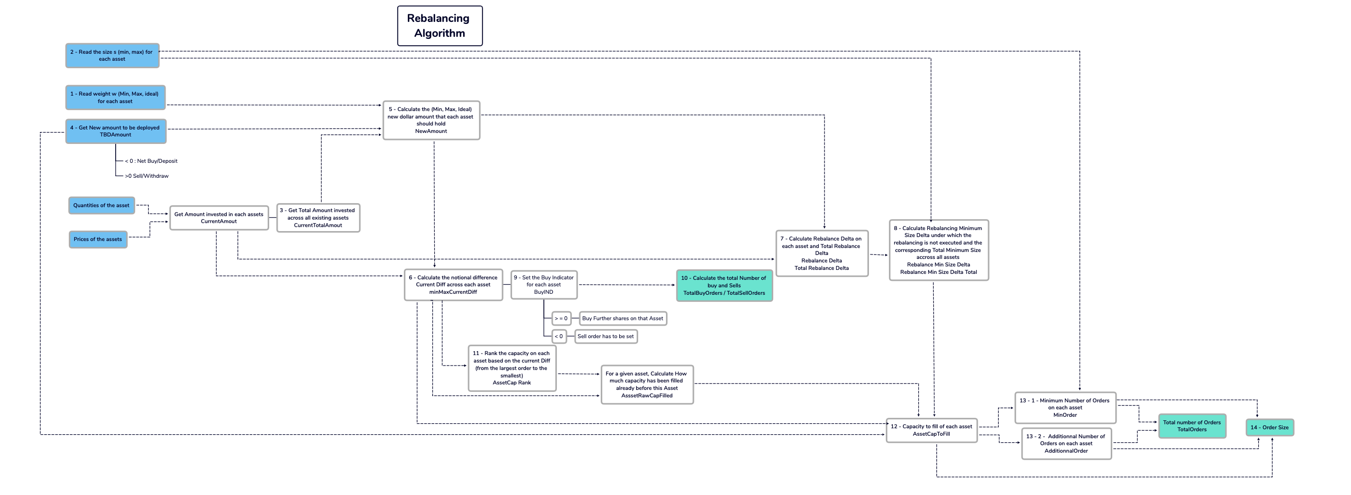
Figure 1: Rebalancing Flow Flow Chart: Cascading Waterfall Round Robin Algorithm

5 Alien vs. Predator, aka, Gas-Fees versus Slippage: Coming Soon To Every Blockchain Network Near You

• In this section we describe in more details the intuitive explanations - regarding the minimum and maximum order size that depend on gas fees and slippage - provided in Section (2.1) to supplement the main algorithm described in Section (3).

5.1 Prequel: David versus Goliath (You against The Markets)

The recent blockbuster book, David and Goliath: Underdogs, Misfits, and the Art of Battling Giants (Gladwell 2013), talks about the advantages of disadvantages, which in the legendary battle refers to (among other things) the nimbleness that David possesses due to his smaller size and lack of armor, that comes in handy while defeating the massive and seemingly unbeatable Goliath. Despite the inspiring tone of the story the efforts of the most valiant financial market participant can seem puny and turn out to be inadequate, as it gets undone when dealing with the gargantuan and mysterious temperament of uncertainty in the markets.

Another main feature of the David versus Goliath story is the tool (sling: End-note 7) that David uses to defeat Goliath. In this section, we hope to provide tools for market participants to contend with the Goliath-like uncertainty in financial markets. A trader’s conundrum is whether (and how much) to trade during a given interval or wait for the next interval when the price momentum is more favorable to his direction of trading. But given the nature of uncertainty in the social sciences, any weapon might prove to be insufficient compared to the sling that delivered the fatal blow to Goliath, until perhaps, one can discern the ability to read the minds of all the market participants. That being said, the techniques in this section will go a long way towards helping participants and making their life easier when confronting the markets. In addition, the mechanisms we provide can be useful for combating uncertainty and aiding better decision making in many areas of the social sciences.

Note that, Slippage is also known as Market Impact. The problem of minimizing slippage by finding an optimal trade size is extensively studied in traditional finance. Numerous models have been developed that provide insights to market participants and deliver a well curated trade execution schedule (Bertsimas & Lo 1998; Almgren & Chriss 2001; Karastilo 2020).

5.2 Checking Block-Busters and Calculating Trading Block-Sizes

The size of all the trades done on a blockchain network have to be optimized so that gas fees and slippage are minimized. If we try to decrease slippage, we will have to do more trades and hence incur higher gas fees. Likewise, if we try to reduce gas fees, by trading bigger executions, we will take on more market impact or slippage.

The trading block size calculations will have to be implemented in a separate technological component. In the initial phases - for simplicity - we can have these block sizes computed in a spreadsheet - or other data store whenever necessary - and we can use it in the algorithm in Section (3). Once the rebalancing portion and weight calculations are performing satisfactorily the focus can shift on rigorous implementation of the trading block size calculations using live data. Optimization of the trading block sizes are less important for now than the weight calculations and rebalancing. A separate calculation procedure will calculate and output the minimum and maximum size of trades across each asset into a data store from which the rebalancing engine will access these values. This size is related to the average daily volume across each asset, average network gas fees and a few other factors. This mechanism which is ideally implemented as an independent portion will need historical market data and generate the block size list. $\left(mins_{it},maxs_{it}\right)$ are the minimum and maximum trading block sizes recommend for asset $i$ at time $t$. In the initial iterations of the platform, the following size calculations will suffice. These will be enhanced later depending on various considerations.

• Input: Historical Market Data and Asset List

• Output: Minimum and Maximum Trading Block Size

  $$mins_{it}=\max\left[\left(AVGGASFEES_{it}\right)*\left(MINSIZEMULTIPLIER_{it}\right),MINSIZEPARAM{}_{it}\right]$$ (54)

  Here, $AVGGASFEES_{it}$, $MINSIZEMULTIPLIER_{it}$ and $MINSIZEPARAM_{it}$ represent respectively, at time $t$, the average gas fees on the network that asset $i$ is part of, a factor to set the order size as a multiple of the average gas fees and a safety parameter to ensure that order sizes are not too small. $\left(MINSIZEMULTIPLIER_{t}=1000\right)$ is a suggested value such that gas fees (implicit transaction costs) will be around 0.1% of the order size. $MINSIZEPARAM_{it}=25000$ in USD terms is a suggested value; but it will generally have to be different across networks. Note that $AVGGASFEES_{it}$, $MINSIZEMULTIPLIER_{it}$ and $MINSIZEPARAM_{it}$ will be the same across many assets. Some indicative gas fees are given in Figure (2).

  $$maxs_{it}=\min\left(\left[\frac{AVGDAILYVOLUME_{it}}{MAXSIZEDIVISOR_{it}}\right],\left[\frac{LIQUIDITYPOOLDEPTH_{it}}{2*\left(MAXSIZEDIVISOR_{it}\right)}\right],MAXSIZEPARAM_{it}\right)$$ (55)

  Here, $AVGDAILYVOLUME_{it}$, $LIQUIDITYPOOLDEPTH_{it}$, $MAXSIZEDIVISOR_{it}$ and

  $MAXSIZEPARAM_{it}$ represent respectively, at time $t$, the average daily volume of asset $i$ on the centralized exchange to which orders for that asset will be sent, the total depth of the liquidity pool from which the asset will be procured or liquidated, a factor to set the order size as a fraction of the daily volume or the liquidity pool depth and a safety parameter to ensure that order sizes are not too large. $\left(MAXSIZEDIVISOR_{it}=1000\right)$ is a suggested value such that the market impact (implicit transaction costs) will be around 0.1% of the transaction costs. Cleary these parameters will be revisited and estimated based on several factors using actual historical data mixed with human instincts. $MAXSIZEPARAM_{it}=200000$ in USD terms is a suggested value; but it will generally have to be different across networks and this default should be such that the maximum slippage is less than 1 percent. Note that $MAXSIZEDIVISOR_{it}$ and $MAXSIZEPARAM_{it}$ will be the same across many assets. Clearly, we can set $MAXSIZEDIVISOR_{it}$ to be different for centralized exchanges and decentralized exchange liquidity pools.

  

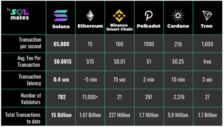
  Source: Introduction To Solana, Chaindebrief Article Link

  Figure 2: Blockchain Network Comparison

• Figure (5) shows the minimum and maximum trade size being used - at the asset level - as part of the rebalancing algorithm in Section (3).

6 Weight Calculation Engine: Obtaining Mathematical Risk Parity

Kashyap (2022) provides more detailed and intuitive explanations to supplement the methodologies described here. The weight calculations will have to be implemented in a separate technological component. Initially - for simplicity - we can have these weights computed in a spreadsheet - or other data store, on demand as necessary- and we can use it in the algorithm in Section (3).

Within the first few weeks of operation, the goal will be to calculate weights weekly or even several times during a week if possible. Once the rebalancing portion is performing satisfactorily the focus can shift to the weight calculation mechanism, which is extremely crucial, and to have it connected to live data feeds. A separate calculation routine will calculate and output the minimum, ideal and maximum weights across each asset into a data store from which the rebalancing engine will access these values. VVV (Velocity of Volatility and Variance) weights will be the core of this engine and our reference weight. This central portion will be mixed with other suitable adjustments to get the overall weights on the assets. The rebalancing mechanism which is ideally implemented as an independent portion will read these weights from the data store and generate the order list. $\left(minw_{it},idealw_{it},maxw_{it}\right)$ are the minimum, ideal and maximum weights recommend for asset $i$ at time $t$.

• Input: Historical Market Data (Daily Open, Close, High, Low Prices) and Asset List

• Output: Minimum, Ideal and Maximum Weights

The following weight calculation methodologies will need to be implemented initially. These can be modified to more sophisticated techniques in subsequent iterations. We need the return, risk (volatility) across each asset and the covariance between each asset pair to calculate the weights for each asset, $i$, in the portfolio at time $t$. The total number of assets in the portfolio is $k_{t}$ assets at time $t$.

6.1 Return and Risk (Volatility) Calculations

The weight calculation depends on calculating the return of asset prices on a daily basis (could be at other frequencies as well, but we start with daily returns). The return will be the continuously compounded measure. The volatility will be the standard deviation of the continuously compounded returns over a historical time period, generally around 90 days. The volatility will need to be calculated on a rolling 90 days basis.

1. Continuously Compounded Return, $R_{t}$, at any time $t$ is given by the logarithm of the ratio of the Price at time $t$, $P_{t}$, and the Price at time $t-1$, $P_{t-1}$, as shown below,

   $$R_{t}=\ln\left(\frac{P_{t}}{P_{t-1}}\right)$$ (56)

2. Volatility at time $t$, $\sigma_{t}$ is calculated as below using the average return, $\bar{R}_{t}$, at time $t$ and then calculating the standard deviation. It can be done directly if suitable libraries are available. $\sigma_{t}^{2}$ is the variance at time $t$. Here, $T=90$ unless otherwise stated.

   $$\bar{R}_{t}=\left(\frac{1}{T}\right)\sum_{i=t}^{t-T}R_{i}$$ (57)

   $$\sigma_{t}^{2}=\left(\frac{1}{T-1}\right)\sum_{i=t}^{t-T}\left(R_{i}-\bar{R}_{t}\right)^{2}$$ (58)

   $$\sigma_{t}=\sqrt{\left(\frac{1}{T-1}\right)\sum_{i=t}^{t-T}\left(R_{i}-\bar{R}_{t}\right)^{2}}$$ (59)

3. Calculate the volatility for the longest historical time period possible for each asset. Possibly for the last 360 days or longer. Some new assets might have a relatively shorter price time series, and it is okay to calculate volatility for those assets for the number of days for which prices are available.

6.2 Asset Weight Calculations

1. Equal Weighted Scenario gives the same weight, $wequal_{it}$, for each asset, $i$, in the portfolio at time $t$. The total number of assets in the portfolio is $k_{t}$ assets at time $t$. This is a fairly robust strategy and performs well under many scenarios and is highly tolerant to estimation errors.

   $$wequal_{it}=\frac{1}{k_{t}}$$ (60)

2. Simple Variance Weighted Scenario gives the weight, $wsimplevar_{it}$, for each asset, $i$, in the portfolio at time $t$. The total number of assets in the portfolio is $k_{t}$ assets at time $t$. This weighting scheme can be shown to give the lowest variance of the portfolio under certain conditions.

   $$wsimplevar_{it}=\left(\frac{\frac{1}{\sigma_{it}^{2}}}{\sum_{j=1}^{k_{t}}\frac{1}{\sigma_{jt}^{2}}}\right)$$ (61)

   Here, $\sigma_{it}^{2}$ is the variance of asset, $i$, at time $t$, calculated using Steps (1; 2) in Section (6.1).

3. Simple Parity Weighted Scenario gives the weight, $wsimpleparity_{it}$, for each asset, $i$, in the portfolio at time $t$. The total number of assets in the portfolio is $k_{t}$ assets at time $t$. This weighting scheme holds when correlations tend to one, which is a reasonable assumption during market crashes. When we set the weights to be inverse of the volatilities divided by the sum of all the inverse volatilities, we get one solution such that the risk contribution from each asset is equal. This solution also satisfies the constraints that the sum of the weights is equal to one and the weights are positive.

   $$wsimpleparity_{it}=\left(\frac{\frac{1}{\sigma_{it}}}{\sum_{j=1}^{k_{t}}\frac{1}{\sigma_{jt}}}\right)$$ (62)

   Here, $\sigma_{it}$ is the volatility of asset, $i$, at time $t$, calculated using Steps (1; 2) in Section (6.1).

4. Risk Parity Weighted Scenario gives the weight, $wriskparity_{it}$, for each asset, $i$, in the portfolio at time $t$. The total number of assets in the portfolio is $k$ assets at time $t$. We remove the time suffix for the number of assets to lighten the notation. This weighting schemes ensures that the risk contribution of each asset towards the overall portfolio risk is equal. The covariance between the assets is also considered in this formulation. Using matrix notation, we can write the variance of the portfolio as,

   $$\boldsymbol{\sigma_{p}\left(w\right)^{2}}=\boldsymbol{w^{\prime}Xw}$$ (63)

   $\boldsymbol{\sigma_{p}^{2}}$ is the portfolio variance which is expressed using the covariance matrix, $\boldsymbol{X}$ of the $k$ individual securities. $\boldsymbol{w}$ is the weight vector to be estimated. One condition on the weights can be that that $\boldsymbol{w^{\prime}1}=1$ Here, $\boldsymbol{1}$ is the column vector (or k*1 matrix) with 1. Simplifying this further, using the condition that the risk contribution from each asset is equal, we arrive at the below formulation, which can be solved using fixed point techniques,

   $$\boldsymbol{w_{i}}=\frac{\boldsymbol{\sigma_{p}\left(w\right)^{2}}}{\boldsymbol{k\left(\sum w\right)_{i}}}$$ (64)

   This is equivalently solved as the below minimization problem,

   $$\underset{\boldsymbol{w}}{\min}\sum_{i=1}^{k}\left(\boldsymbol{w_{i}}-\frac{\boldsymbol{\sigma_{p}\left(w\right)^{2}}}{\boldsymbol{k\left(\sum w\right)_{i}}}\right)$$ (65)

   A python library to solve the above problem, and to calculate the risk Parity weights, is available at this location: (Risk Parity Portfolio, Python Library). The corresponding R package is available at this location: (Risk Parity Portfolio, R Library; Risk Parity Portfolio, R Reference PDF).

5. Velocity of Volatility and Variance or Volatility of Volatility and Variance (VVV) Scenario gives the weight, $wvvv_{it}$, for each asset, $i$, in the portfolio at time $t$. The total number of assets in the portfolio is $k_{t}$ assets at time $t$. In this scenario, we adjust the volatilities higher by the volatility of the volatilities of each asset. This weighting scheme holds when correlations tend to one, which is a reasonable assumption during market crashes. When we set the weights to be inverse of the adjusted volatilities divided by the sum of all the inverse adjusted volatilities, we get one solution such that the risk contribution from each asset is equal. This solution also satisfies the constraints that the sum of the weights is equal to one and the weights are positive. We first use the formulae in Steps (1; 2) in Section (6.1), along with similar notation, to calculate the volatility of volatility as follows,

   $$V_{it}=\ln\left(\frac{\sigma_{it}}{\sigma_{i,t-1}}\right)$$ (66)

   $$\bar{V}_{it}=\left(\frac{1}{T}\right)\sum_{l=t}^{t-T}V_{il}$$ (67)

   $$\sigma_{it}^{VVVFactor}=\sqrt{\left(\frac{1}{T-1}\right)\sum_{l=t}^{t-T}\left(V_{il}-\bar{V}_{it}\right)^{2}}$$ (68)

   $$\sigma_{it}^{VVV}=\sigma_{it}+\left(\theta\right)\sigma_{it}^{VVVFactor}$$ (69)

   Here, $\theta$, is a parameter that has to be calibrated to give the length of time a market downturn occurs. We set $\theta=1$ for now and we can consider further estimates of $\theta$ in later iterations.

   $$wvvv_{it}=\left(\frac{\frac{1}{\sigma_{it}^{VVV}}}{\sum_{j=1}^{k_{t}}\frac{1}{\sigma_{jt}^{VVV}}}\right)$$ (70)

   The ideal weight $idealw_{it}$ mentioned in Algorithm (1) corresponds to the weights calculated using this procedure.

6. Covariance Weighted Scenario gives the weight, $wcovar_{it}$, for each asset, $i$, in the portfolio at time $t$. The total number of assets in the portfolio is $k_{t}$ assets at time $t$. We remove the time suffix for the number of assets to lighten the notation. These are the traditional Markowitz inspired portfolio theory weights. The weight, $wcovar_{it}$ for each asset, $i$ is given by using the corresponding row in the weight vector derived below. Consider a portfolio variance optimization problem, shown using matrix notation, in Equation (71). $\boldsymbol{\sigma_{p}^{2}}$ is the portfolio variance which is expressed using the covariance matrix, $\boldsymbol{X}$ of the $k$ individual securities. $\boldsymbol{w}$ is the weight vector to be estimated with the condition that $\boldsymbol{w^{\prime}1}=1$. Here, $\boldsymbol{1}$ is the column vector (or k*1 matrix) with 1.

   $$\boldsymbol{\sigma_{p}^{2}}=\boldsymbol{w^{\prime}Xw}\qquad;\boldsymbol{w^{\prime}1}=1$$ (71)

   Minimizing variance using Lagrangian multiplier techniques gives the following weights,

   $$\boldsymbol{w}=\frac{\boldsymbol{X^{-1}1}}{\boldsymbol{1^{\prime}X^{-1}1}}$$ (72)

   Note that several alternate constrained optimizations are possible and there is a detailed discussion of the issues that arise with constrained optimizations in Kashyap (2022). The limitations of optimization methodologies and the need for range based techniques, which introduce randomness in the decision process are discussed in detail in the series, “Fighting Uncertainty with Uncertainty”: (End-note 8; Kabeer 2016).

7. To get a weight range for each asset, we need a minimum and maximum weight. The minimum and maximum weights for each asset will be arrived at using the below formulae.

   $$minweight_{it}=\max\left[\min\left(All\>Weights\>For\>Asset\>i\right),\min\left(wvvv_{it},MINASSETWEIGHT_{t}\right)\right]$$ (73)

   $$maxweight_{it}=\min\left[\max\left(All\>Weights\>For\>Asset\>i\right),\max\left(wvvv_{it},MAXASSETWEIGHT_{t}\right)\right]$$ (74)

   Here, $MINASSETWEIGHT_{t}$ and $MAXASSETWEIGHT_{t}$ are based on risk management guidelines which will also be reviewed and revised continuously. Suggested values to start with are $MINASSETWEIGHT_{t}=0.0$ and $MAXASSETWEIGHT_{t}=0.15$. We will consider several other weight calculation techniques in later stages. Further fine tuning of the range for each asset will be based on these additional weight calculations, observed empirical performance and other additional considerations. The minimum and maximum weights $\left(minw_{it},maxw_{it}\right)$ mentioned in Algorithm (1) correspond to the weights calculated using this procedure.

8. An initial simplification can be to calculate weights on each network separately. This is related to limitations on bridge capacities and related bottlenecks (Kashyap 2023). This means that we will have weights optimized for each network. Hence, instead of relying on global portfolio weights and arriving at network weights from the global portfolio weights, we will calculate weights on each network by considering it to be a global portfolio.

9. Figures (3; 4) show weights being calculated using different techniques and how we arrive at the minimum and maximum capacity - at the asset level - as part of the rebalancing algorithm in Section (3). Several other weighting mechanisms are possible and much further research can be conducted in this domain - seeking to improve portfolio performance - and can be implemented progressively at conducive times. These additional weighting techniques can either replace or can be included as an extra weight before choosing the minimum and maximum for each asset.

7 Numerical Results

Each of the tables in this section are referenced in the main body of the article. Below, we provide supplementary descriptions for each table.

• The Table in Figure (3) shows numerical examples related to the weight calculations described in Section (6) and the material in Section (6.2). The numbers in the figure also show the volatility and variance at the asset level. Certain control parameters are also given such as the net inflow or outflow into the fund. We have a spreadsheet, which can be shared upon request, wherein the control variables can be changed to see how the cascading algorithm performs - by observing several intermediate variables that are calculated - and compare it to a simple rebalancing rule.

• The asset weights shown in the illustrations are based on real historical asset prices. The full data sample consists of daily observations from October 31, 2020 to October 31, 2021. The asset names used are based on naming conventions followed by most crypto data providers (End-note 5; 5a). The USD suffix in the asset name indicates that the prices were denominated in US Dollars. The asset prices are expressed in stable coins such as USDT or USDC which are pegged to the US dollar (Ante, Fiedler & Strehle 2021; End-note 9).

• The simple rebalancing mechanism considers the difference between the ideal notional that an asset should hold and the amount it currently holds to arrive at the whether buy or sell orders need to be made. In contrast, the cascading rebalancing mechanism considers the different between the minimum notional that an asset should hold - or the maximum notional amount an asset can hold depending on whether there is a net deposit or withdrawal from the portfolio - and the amount it currently holds to arrive at the whether buy or sell orders need to be made. Numerous simulation based comparisons can be included either in appendix of this paper or will be provided in a subsequent paper that will have more analytical estimates and performance results.

• The columns in Figure (3) represent the following information respectively:

  1. AssetName is the symbol or asset name that is part of the portfolio being rebalanced.

  2. Volatility is the volatility of the corresponding asset.

  3. vvvFactor corresponds to the calculation of asset weights based on the Velocity of Volatility and Variance technique described in Section (6.2).

  4. VVV refers to the VVV adjusted volatility of the asset.

  5. Variance is the variance of the corresponding asset.

  6. EqualWeight is the weight allocated to the asset based on the equal weighting technique. This is discussed in Point (1) in Section (6.2).

  7. MinVarianceWeight is the weight allocated to the asset such that the variance of the portfolio is minimized. This is discussed in Point (6) in Section (6.2).

  8. SimpleParityWeight is the weight allocated to the asset based on the simple parity scheme. This is discussed in Point (3) in Section (6.2).

  9. vvvWeight is the weight allocated to the asset based on the VVV weighting technique. This is discussed in Point (5) in Section (6.2).

  10. riskParityWeight is the weight allocated to the asset based on the risk parity weighting technique. This is discussed in Point (4) in Section (6.2).

  11. riskParityWeight-2% is 2% less than the weight in the risk parity weighting technique.

  12. riskParityWeight+2% is 2% more than the weight in the risk parity weighting technique.

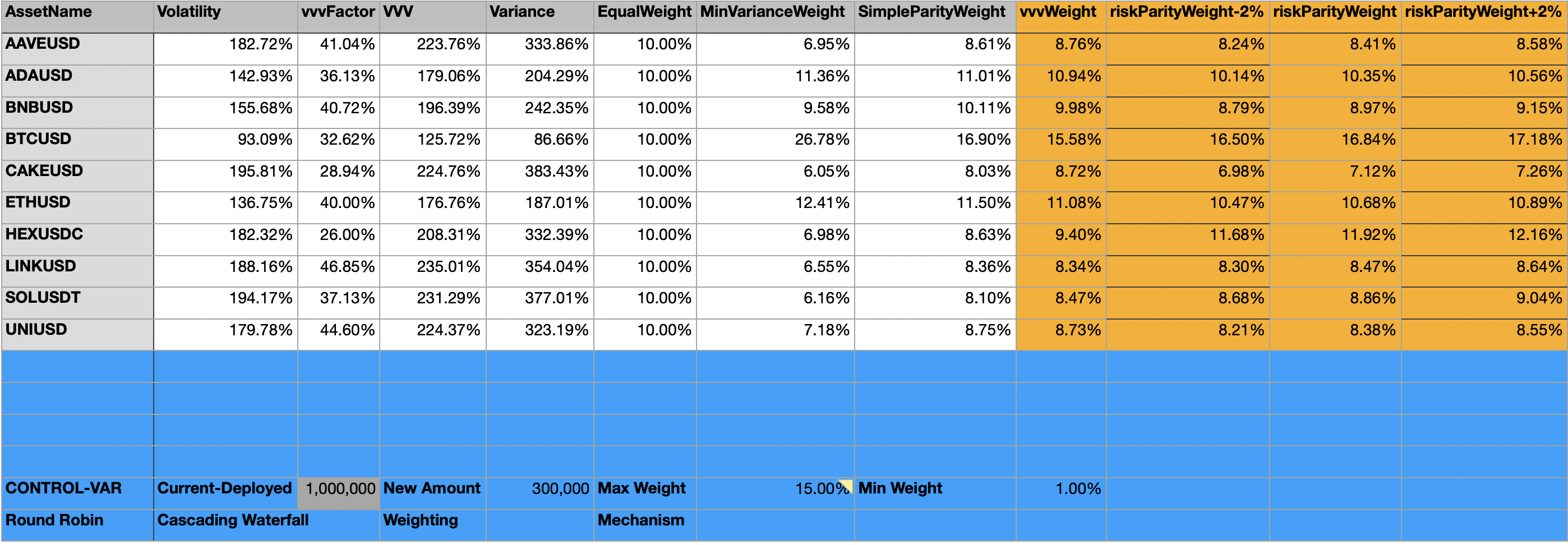
Figure 3: Rebalancing Illustration: Asset Weights

• The Table in Figure (4) shows numerical examples related to how we arrive at the minimum and maximum capacity for each asset, which is expressed in terms of the notional amounts each asset can hold. The difference between asset capacities and the current notional amounts deployed across each asset - also given in the illustration - determine whether an asset will receive new funds or funds will be withdrawn when there are net inflows and outflows into the fund.

• The columns in Figure (4) represent the following information respectively:

  1. minMaxWeight is the weight allocated to the asset such that the variance of the portfolio is minimized but where there are minimum and maximum weight constraints set for each asset. The variance minimization of the portfolio and the corresponding method to derive asset weights is discussed in Point (6) in Section (6.2). The minimum and maximum constraint across each asset is set at 0% and 15% respectively.

  2. noShortWeight is the weight allocated to the asset such that the variance of the portfolio is minimized but when no shorts are allowed across any asset. This corresponds to not having a maximum weight constraint on any asset but having a zero percent minimum level. The variance minimization of the portfolio and the corresponding method to derive asset weights is discussed in Point (6) in Section (6.2).

  3. minWeightAlt is the minimum weight based on the minimum and maximum weight bounds given in Figure (3). This weight is obtained after selecting the minimum and maximum based on the weighting techniques discussed in Section (6.2) and Figure (3).

  4. minWeight is the minimum weight based on selecting the minimum across the various weighting techniques discussed in Section (6.2) and Figure (3).

  5. idealWeight is obtained using the VVV weighting technique. This is discussed in Point (5) in Section (6.2).

  6. maxWeight is the maximum weight based on selecting the maximum across the various weighting techniques discussed in Section (6.2) and Figure (3).

  7. trueMinWeight is the minimum weight without using the minimum weight bound given in Figure (3).

  8. minNotionalCurrent is the minimum notional capacity of the asset based on the minimum weight of the corresponding asset and the total current amount invested in the portfolio plus net deposits or withdrawals to be made across all investors.

  9. idealNotionalCurrent is the ideal notional capacity of the asset based on the ideal weight of the corresponding asset and the total current amount invested in the portfolio plus net deposits or withdrawals to be made across all investors.

  10. maxNotionalCurrent is the maximum notional capacity of the asset based on the maximum weight of the corresponding asset and the total current amount invested in the portfolio plus net deposits or withdrawals to be made across all investors.

  11. actualNotionalCurrent is the actual amount invested into the corresponding asset.

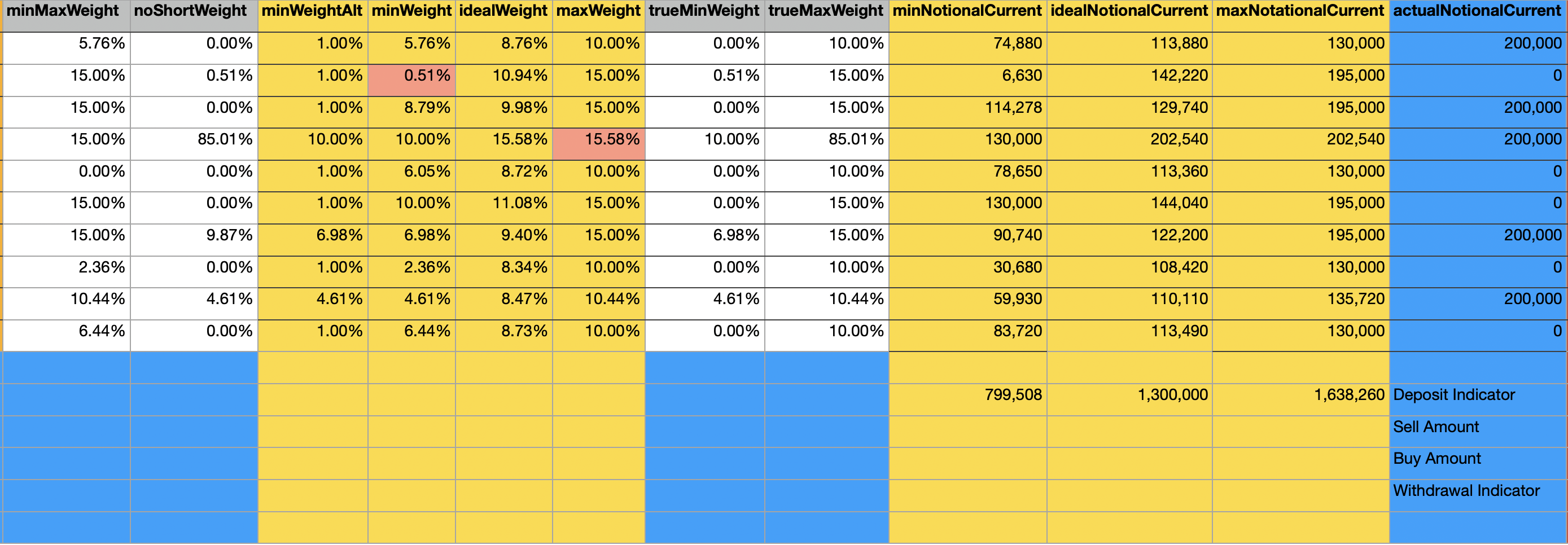
Figure 4: Rebalancing Illustration: Current Notional Amounts

• The Table in Figure (5) shows numerical examples related to the minimum and maximum trade size calculations described in Section (5.2) based on the material in Section (5) regarding the trade-off between gas fees and trading slippage. This figure also illustrates the order schedule based on a simple rebalancing rule when trades are generated as assets move away from their intended weights.

• The columns in Figure (5) represent the following information respectively:

  1. idealActualNotionalDiff is the difference between the ideal notional capacity of the asset and the actual amount invested in the asset.

  2. absIdealActDiff is the difference between the ideal notional capacity of the asset and the actual amount invested in the asset.

  3. newMinDeploy is the minimum notional amount that should be deployed - or invested - into this asset based on the minimum weight of the corresponding asset and the net deposits or withdrawals to be made across all investors.

  4. newIdealDeploy is the ideal notional amount that should be deployed - or invested - into this asset based on the ideal weight of the corresponding asset and the net deposits or withdrawals to be made across all investors.

  5. newMaxDeploy is the maximum notional amount that should be deployed - or invested - into this asset based on the maximum weight of the corresponding asset and the net deposits or withdrawals to be made across all investors.

  6. minBlockSize is the minimum trade size for this asset based on the calculations described in Section (5.2).

  7. maxBlockSize is the maximum trade size for this asset based on the calculations described in Section (5.2).

  8. minNumberOrders is the minimum number of orders that need to be made on this asset based on the simple rebalancing mechanism described above Figure (3). This column shows zero - 0- if the absolute Value of difference between ideal and actual notional is less than the minimum block size; and 1 otherwise.

  9. minBlockSizeInd indicates that the trade size on this asset is below the minimum trade size for that asset. This column shows minus one, -1, if the absolute Value of the difference between ideal and actual notional is less than minimum block size; 1 otherwise.

  10. additionalOrders is the number of additional orders required to fill the total deficit in this asset. This is the number of orders in addition to the minimum number of orders indicated by minNumberOrders.

  11. Buy or Sell indicates if we are making buy or sell trades on this asset.

  12. totalOrders indicates the total number of orders to be made on this asset.

  13. orderSize is the size of each trade to be made on this asset.

  14. orderSchedule indicates the sequence in which trades for this asset will have to be executed in comparison to the other assets in the portfolio.

  15. amountDeployed indicates the total amount deployed on this asset in this rebalancing event. This is the product of totalOrders and orderSize.

  16. cummTotalDeployed indicates the cumulative total deployed - summing up the amounts invested or withdrawn, bought or sold - across all the assets in the portfolio starting from the asset in the first row.

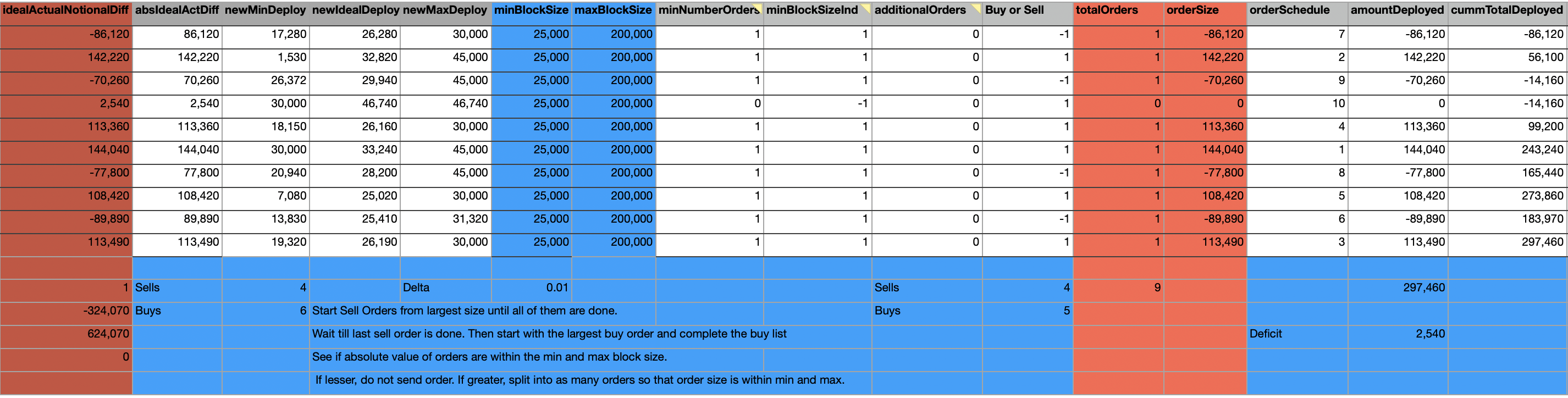
Figure 5: Rebalancing Illustration: Simple Mechanism Order Schedule

• The Table in Figure (6) shows intermediate variables related to the calculations based on the material described in Section (3) corresponding to the steps in Algorithm (1). This figure also gives a capacity ranking of the assets depending on how much funds they can hold. Assets that need to reduce their holdings - or those that generate sell orders - are higher up in the capacity list and then assets which require inflows show up next - both in decreasing absolute value of dollar amounts.

• The columns in Figure (6) represent the following information respectively:

  1. minMaxActualNotionalDiff is the difference between either the minimum or maximum notional capacity of the asset and the actual amount invested in the asset. This is explained in Step (6) of Algorithm (1) in Section (3).

  2. rebalanceDelta indicates that for the corresponding asset there is a need add to the existing position even if there is a net withdrawal and vice versa. This is explained in Steps (7; 8) of Algorithm (1) in Section (3).

  3. buyIndicator indicates that we need to buy additional positions for this asset. This is explained in Step (9) of Algorithm (1) in Section (3).

  4. capRankCrudeDec indicates the ranking for this asset based on capacity while comparing with all the other assets in the portfolio in decreasing order. This is explained in Step (11) of Algorithm (1) in Section (3).

  5. capRankCrudeDec indicates the ranking for this asset based on capacity while comparing with all the other assets in the portfolio in increasing order. This is explained in Step (11) of Algorithm (1) in Section (3).

  6. capacityRank indicates the ranking for this asset based on capacity while comparing with all the other assets in the portfolio with the largest sells in decreasing order first and then largest buys in decreasing order next. This is explained in Step (11) of Algorithm (1) in Section (3).

  7. rawCapacityAlreadyFilled is an intermediate variable used to arrive at the capacity to fill - capacityToFill - on that asset. This is explained in Step (12) of Algorithm (1) in Section (3).

  8. capacityAlreadyFilled is an intermediate variable used to arrive at the capacity to fill - capacityToFill - on that asset. This is explained in Step (12) of Algorithm (1) in Section (3).

  9. rawCapacityInclusive is an intermediate variable used to arrive at the capacity to fill - capacityToFill - on that asset. This is explained in Step (12) of Algorithm (1) in Section (3).

  10. capacityInclusive is an intermediate variable used to arrive at the capacity to fill - capacityToFill - on that asset. This is explained in Step (12) of Algorithm (1) in Section (3).

  11. capacityIndicator is an intermediate variable used to arrive at the capacity to fill - capacityToFill - on that asset. This is explained in Step (12) of Algorithm (1) in Section (3).

  12. capacityToFill indicates the capacity to fill on the corresponding asset based on the difference between the current amount on each asset and maximum capacity on the asset, while taking into account the total new amount to be deployed or withdrawn. This is explained in Step (12) of Algorithm (1) in Section (3).

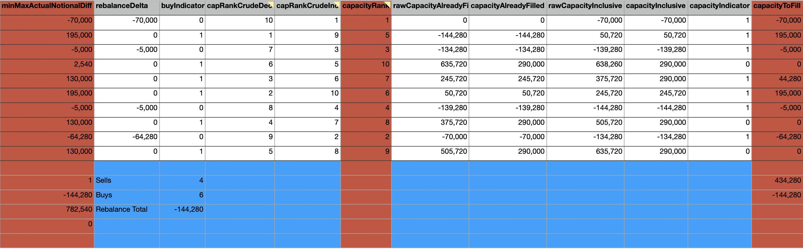
Figure 6: Rebalancing Illustration: Cascading Mechanism Capacity To Fill

• The Table in Figure (7) shows numerical examples related to the order schedule generated for the cascading rebalancing mechanism in Algorithm (1) based on the material in Section (3). This figure illustrates the number of trades and the size of each trade across each asset. Sell orders are sent first followed by buy orders since the amount received from selling assets is required for investment into assets that require additional inflows.

• The columns in Figure (7) represent the following information respectively:

  1. AbsCapacityToFill corresponds to each rebalance event corresponding to

  2. minNumberOrders is the minimum number of orders that need to be made on this asset based on the cascading rebalancing mechanism described in Algorithm (1) in Section (3). This column shows zero - 0- if the absolute Value of capacity to fill is less than minimum block size; and 1 otherwise. This is explained in Step (13) of Algorithm (1) in Section (3).

  3. minBlockSizeInd indicates that the trade size on this asset is below the minimum trade size for that asset. This column shows minus one, -1, if the absolute Value of capacity to fill is less than minimum block size; 1 otherwise.

  4. additionalOrders is the number of additional orders required to fill the total deficit in this asset. This is the number of orders in addition to the minimum number of orders indicated by minNumberOrders. This is explained in Step (13) of Algorithm (1) in Section (3).

  5. Buy or Sell indicates if we are making buy or sell trades on this asset.

  6. totalOrders indicates the total number of orders to be made on this asset. This is the sum of minNumberOrders and additionalOrders. This is explained in Step (13) of Algorithm (1) in Section (3).

  7. orderSize is the size of each trade to be made on this asset. This is explained in Step (14) of Algorithm (1) in Section (3).

  8. orderSchedule indicates the sequence in which trades for this asset will have to be executed in comparison to the other assets in the portfolio.

  9. amountDeployed indicates the total amount deployed on this asset in this rebalancing event. This is the product of totalOrders and orderSize.

  10. cummTotalDeployed indicates the cumulative total deployed - summing up the amounts invested or withdrawn, bought or sold - across all the assets in the portfolio starting from the asset in the first row.

  11. altCapacityToFill is an alternative calculation to find the capacity to fill - capacityToFill in Figure (6) - on the corresponding asset based on the difference between the current amount on each asset and maximum capacity on the asset, while taking into account the total new amount to be deployed or withdrawn. This is explained in Step (12) of Algorithm (1) in Section (3).

  12. altMinNumberOfOrders is an alternative calculation to find the minimum number of orders - minNumberOrders in Figure (6) - but with the difference that orders are counted only when the quantities are within the minimum and maximum trade size. That is if the quantity to be traded on the asset is less than the minimum trade size, it is not considered as an order.

  13. rebalanceDeltaAdusted indicates the rebalance delta - rebalanceDelta in Figure (6) - on the asset by taking into account the alternate minimum number of orders, altMinNumberOfOrders.

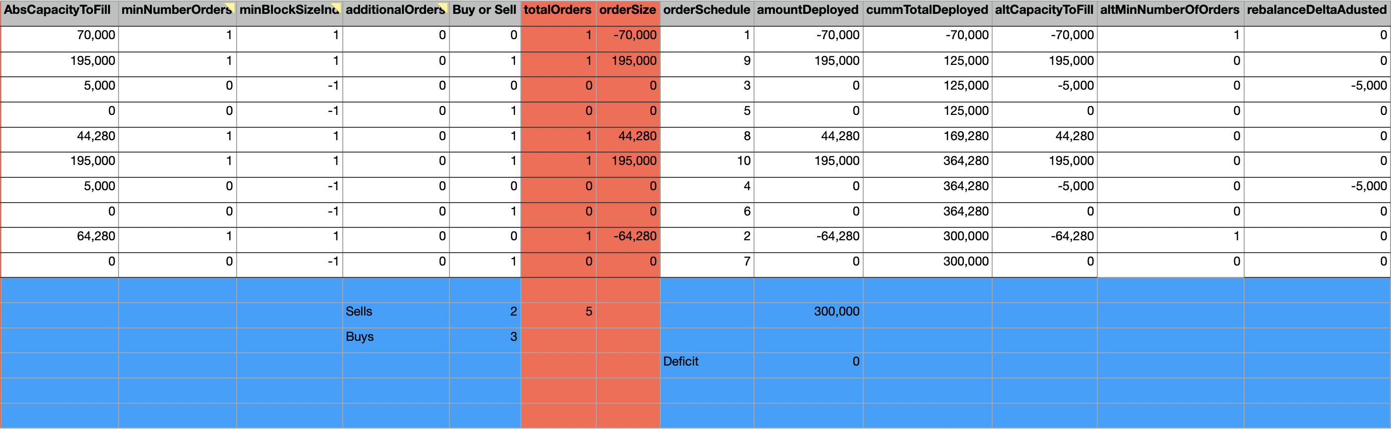
Figure 7: Rebalancing Illustration: Cascading Mechanism Order Schedule

8 Implementation Pointers and Areas for Further Research

The two components - calculation of asset capacities and the rebalancing methodology described in this paper - are some of the earliest pieces that need to be built, and tested, to understand how well they apply to various investment mandates and how seamlessly they would work in a blockchain environment. Once these initial efforts have proved satisfactory, attempting to make improvements is quite natural. If any investment firm has to approach the implementation in terms of phases, it would be prudent in the initial phase to ensure these techniques could be invoked and utilized on an on-demand basis. The next set of enhancements are to be able to connect them to live data updates, and completely automate them, so that these calculations can run on a daily basis or even several times during a 24 hour period.

The rebalancing algorithm can be a stand alone component - external to the blockchain system - that reads the investment variables and outputs the trade schedule for each asset, which will be used by fund personnel to perform the necessary trades. The trades need to happen on the blockchain environment, but the calculations for the steps in the rebalancing algorithm can be done in off-chain scripts. The weight calculation engine will be a separate component which interact with the rebalancing calculation routines and provides the relevant information to the portfolio teams. A similar stand-alone component can perform the minimum and maximum trade size calculations. This ensures that each piece can be enhanced without affecting the other components.

Numerous alternative weight calculation techniques are possible. We have used the closing prices to calculate the weights. But open, high or low prices for a particular day can be used instead of the close prices to get alternate weights. The rebalancing algorithm looks at the difference between current amounts invested in an asset from the minimum and maximum capacities, instead we how the ideal capacities vary from the current amounts - based on the ideal weights of the asset - to get the trades to be done on any asset. Again the choice of which approach should depend on how often we plan to rebalance and how closely we wish to stay aligned with the calculated weights and the extent of forecast errors that persist in the operating environment.

To govern a system with many moving parts, such as the one described in this paper, several parameters need to be monitored and tweaked on a regular basis. The portfolio management team will have to observe these parameters continuously and update them, as necessary, using specialized internal tools. The bulk of the configurations that decide how the system will run on a periodic basis are related to asset capacities and trade executions. In addition, trade executions can be error prone wherein failures need to be monitored and intelligent customizations to retry need to be incorporated into the process. Hence trade execution related parameters and operational procedures will garner significant focus and a big chunk of time from the investment team.

Internal tools have to be designed such that the flow of funds happens automatically, for the most part, with human intervention to complement the decision making. Significant automation of the investment apparatus will allow the fund to take advantage of market opportunities seamlessly and human oversight will enable the team to watch out for exceptional situations and fine tune the decisions. This coupling of man and machine will lead to a better final outcome for all our participants.

An illustration of this pairing is that the approach we have described to investing on blockchain will benefit from volatility, which is seen as the bane of crypto markets by most players. Volatility, which is the up and down movement of asset prices, will cause our rebalancing algorithm to buy assets that drop in prices and sell assets as they start soaring again. But to filter out the noise and react only to real signals, the buying and selling happens only when certain boundaries or range thresholds are crossed. This spectrum over which transactions happen are automatically calculated based on asset properties, but have to be fine tuned by investment specialists. Suffice it to say, while mathematical optimization techniques offer powerful venues to garner profits, they might fall short of conquering the extreme scenarios that markets present. Hence mixing mathematics models with human intuition, that takes care of exceptional cases, is the ideal recipe for wealth creation.

Our rebalancing methodology will significantly outperform any simple rebalancing mechanism (without minimum and maximum weights on assets) over time in terms of gas fees savings and market impact costs. It could under-perform the simple mechanism when new assets are being added and removed frequently. The underperformance is small compared to the benefits. The algorithm we have designed will provide better performance when the number of assets increases. The algorithm performance will converge to any simple rebalancing mechanism when the minimum and maximum weights on the assets get closer to one another. Quantitative bounds and other analytical results will be provided in a later paper since this paper has a lot of innovations and material already. But if necessary, we can include some of the mathematical estimates as propositions - with the proofs provided in the appendix of this paper or in the related paper.

For the sake of brevity, we have focused on the central elements of our technique. The actual technical implementation will have to cover several specialized scenarios, nuances or other constraints. Additional checks pertaining to division by zero and other such cases need to be considered in the software coding and testing (End-note 10).

9 Conclusions

We have designed a rebalancing algorithm that is tailored for the nuances of blockchain based trading and portfolio management. Our rebalancing mechanism recommends an ideal size and number of trades for each asset, factoring in the gas fee and slippage. The essence of the model we have created gives indications regarding whether trades should be made on individual assets depending on the uncertainty in the micro - asset level characteristics - and macro - aggregate market factors - environments.

The algorithm is presented as a sequence of steps with detailed explanations for the computations that happen in each step and the rationale for performing those calculations. We have provided several numerical examples to illustrate the various steps - including the calculation of numerous intermediate variables - of our rebalancing approach. The Algorithm we have developed can be easily applied outside blockchain to investment funds across all asset classes at any trading frequency and rebalancing duration. In the hyper-volatile crypto market, our approach to daily rebalancing will benefit from volatility. Price movements will cause our algorithm to buy assets that drop in prices and sell as they soar. In fact, the buying and selling happen only when certain boundaries are crossed in order to weed out any market noise and ensure sound trade execution.

We have also shown different ways to calculate portfolio weights and the minimum and maximum trade sizes on an asset that depend on the blockchain network and the properties of the asset. The asset weights and minimum and maximum trade sizes act as inputs to the rebalancing algorithm which then outputs the number of trades on each asset and the size of each trade. We have given detailed mathematical formulations, and technical pointers, to be able to implement the algorithm and its related components as stand-alone technical pieces. Each piece receives information from the blockchain decentralized ledger - and other independent external data sources - to perform its designated calculations. The result of the calculations aid the investment strategy in maintaining its preferred risk and return objectives. Careful orchestration among mathematical optimization for portfolio construction, trade automation of the investment apparatus, and human oversight will allow us to watch out for exceptional situations and ultimately lead to better risk management - which is very much the need of the hour for the decentralized financial landscape.

10 Explanations and End-notes

1. To be, or not to be" is the opening phrase of a soliloquy given by Prince Hamlet in the so-called "nunnery scene" of William Shakespeare’s play Hamlet, Act 3, Scene 1. (William Shakespeare: William Shakespeare, Wikipedia Link)

   To be, or not to be, that is the question:

   Whether ’tis nobler in the mind to suffer

   The slings and arrows of outrageous fortune,

   Or to take Arms against a Sea of troubles,

   And by opposing end them: to die, to sleep …

2. In finance and investing, rebalancing of investments (or constant mix) is a strategy of bringing a portfolio that has deviated away from one’s target asset allocation back into line. Rebalancing Investments, Wikipedia Link

3. In finance, risk factors are the building blocks of investing, that help explain the systematic returns in equity market, and the possibility of losing money in investments or business adventures. Risk Factor (finance), Wikipedia Link

4. Decentralized finance (often stylized as DeFi) offers financial instruments without relying on intermediaries such as brokerages, exchanges, or banks by using smart contracts on a blockchain. Decentralized Finance (DeFi), Wikipedia Link

5. CoinMarketCap is a leading price-tracking website for crypto-assets in the cryptocurrency space. Its mission is to make crypto discoverable and efficient globally by empowering retail users with unbiased, high quality and accurate information for drawing their own informed conclusions. It was founded in May 2013 by Brandon Chez. CoinMarketCap, Website Link

   1. A ranking of cryptocurrencies, including symbols for the various tokens, by market capitalization is available on the CoinMarketCap website. We are using the data as of May-25-2022, when the first version of this article was written. CoinMarketCap Cryptocurrency Ranking, Website Link

6. The following are the four main types of blockchain decentralized financial products or services. These are sometimes collectively referred to as vaults since it requires additional steps to withdraw funds from them. We can also consider them as the main types of yield enhancement, or return generation, vehicles available in decentralized finance:

   1. Single-Sided Staking: This allows users to earn yield by providing liquidity for one type of asset, in contrast to liquidity provisioning on AMMs, which requires a pair of assets. Single Sided Staking, SuacerSwap Link

      1. Bancor is an example of a provider who supports single sided staking. Bancor natively supports Single-Sided Liquidity Provision of tokens in a liquidity pool. This is one of the main benefits to liquidity providers that distinguishes Bancor from other DeFi staking protocols. Typical AMM liquidity pools require a liquidity provider to provide two assets. Meaning, if you wish to deposit "TKN1" into a pool, you would be forced to sell 50% of that token and trade it for "TKN2". When providing liquidity, your deposit is composed of both TKN1 and TKN2 in the pool. Bancor Single-Side Staking changes this and enables liquidity providers to: Provide only the token they hold (TKN1 from the example above) Collect liquidity providers fees in TKN1. Single Sided Staking, Bancor Link

   2. AMM Liquidity Pairs (AMM LP): A constant-function market maker (CFMM) is a market maker with the property that that the amount of any asset held in its inventory is completely described by a well-defined function of the amounts of the other assets in its inventory (Hanson 2007). Constant Function Market Maker, Wikipedia Link

      This is the most common type of market maker liquidity pool. Other types of market makers are discussed in Mohan (2022). All of them can be grouped under the category Automated Market Makers. Hence the name AMM Liquidity Pairs. A more general discussion of AMMs, without being restricted only to the blockchain environment, is given in (Slamka, Skiera & Spann 2012).

   3. LP Token Staking: LP staking is a valuable way to incentivize token holders to provide liquidity. When a token holder provides liquidity as mentioned earlier in Point (6b) they receive LP tokens. LP staking allows the liquidity providers to stake their LP tokens and receive project tokens tokens as rewards. This mitigates the risk of impermanent loss and compensates for the loss. Liquidity Provider Staking, DeFactor Link

      1. Note that this is also a type of single sided staking discussed in Point (6a). The key point to remember is that the LP Tokens can be considered as receipts for the crypto assets deposits in an AMM LP Point (6b). These LP Token receipts can be further staked to generate additional yield.

   4. Lending: Crypto lending is the process of depositing cryptocurrency that is lent out to borrowers in return for regular interest payments. Payments are typically made in the form of the cryptocurrency that is deposited and can be compounded on a daily, weekly, or monthly basis. Crypto Lending, Investopedia Link; DeFi Lending, DeFiPrime Link; Top Lending Coins by Market Capitalization, Crypto.com Link.

      1. Crypto lending is very common on decentralized finance projects and also in centralized exchanges. Centralized cryptocurrency exchanges are online platforms used to buy and sell cryptocurrencies. They are the most common means that investors use to buy and sell cryptocurrency holdings. Centralized Cryptocurrency Exchanges, Investopedia Link

      2. Lending is a very active area of research both on blockchain and off chain (traditional finance) as well (Cai 2018; Zeng et al., 2019; Bartoletti, Chiang & Lafuente 2021; Gonzalez 2020; Hassija et al., 2020; Patel et al. , 2020).

      3. Lending is also a highly profitable business in the traditional financial world (Kashyap 2022). Investment funds, especially hedge funds, engage in borrowing securities to put on short positions depending on their investment strategies.Long only investment funds typically supply securities or lend their assets for a fee.

      4. In finance, a long position in a financial instrument means the holder of the position owns a positive amount of the instrument. Long Position in Finance, Wikipedia Link

      5. In finance, being short in an asset means investing in such a way that the investor will profit if the value of the asset falls. This is the opposite of a more conventional "long" position, where the investor will profit if the value of the asset rises. Short Position in Finance, Wikipedia Link

7. A sling is a projectile weapon typically used to throw a blunt projectile such as a stone, clay, or lead "sling-bullet". It is also known as the shepherd’s sling. Sling (Weapon), Wikipedia Link

8. The range based models we have outlined for the weights are based on a wider set of techniques termed: Randoptimization. The limitations of optimization methodologies and the need for range based methodologies - which introduce randomness in the decision process - are discussed in detail in the series: “Fighting Uncertainty with Uncertainty” Kabeer (2016). The minimum and maximum asset weights we have discussed in the main text are based on this idea of operating a system within a range as opposed to pinning down operational parameters to a single value. The range of values is prudent to use due to the errors that exist around the estimates we obtain for an ideal value. Clearly, the weight range we can use to minimize rebalancing requirements is dependent upon the estimation errors in the corresponding weight optimization process. Conversely, depending on the extent to which we wish to undertake rebalancing - that is how often and the size of trades in comparison to the holdings in the portfolio - we can decide the width of the range we can tolerate for the weights.

9. A Stablecoin is a type of cryptocurrency where the value of the digital asset is supposed to be pegged to a reference asset, which is either fiat money, exchange-traded commodities (such as precious metals or industrial metals), or another cryptocurrency. Stable Coin, Wikipedia Link

10. We would like to highlight the following points to help with the actual coding of the software (Boehm 1983; Balci 1995; Desikan & Ramesh 2006; Green & Ledgard 2011; Knuth 2014). The algorithm we have provided acts mostly as detailed implementation guidelines. Many cases and error conditions need to be handled appropriately during implementation. Alternate implementation simplifications, time conventions, and counters are possible and can be accommodated accordingly. There might even be some issues - or bugs - with the variables, counters and timing. These are due to limitations of not actually testing scenarios using a full fledged software system. But the gist of what we have provided should carry over to the coding stage with very little changes. Conditional statements such as - if … then … else - can be used depending on the implementation language and other efficiency considerations as necessary.

11 References

• Almgren, R., & Chriss, N. (2001). Optimal execution of portfolio transactions. Journal of Risk, 3, 5-40.

• An, Z., Chen, C., Li, D., & Yin, C. (2021). Foreign institutional ownership and the speed of leverage adjustment: International evidence. Journal of Corporate Finance, 68, 101966.

• Ante, L., Fiedler, I., & Strehle, E. (2021). The influence of stablecoin issuances on cryptocurrency markets. Finance Research Letters, 41, 101867.

• Balci, O. (1995, December). Principles and techniques of simulation validation, verification, and testing. In Proceedings of the 27th conference on Winter simulation (pp. 147-154).

• Bartoletti, M., Chiang, J. H. Y., & Lafuente, A. L. (2021). SoK: lending pools in decentralized finance. In Financial Cryptography and Data Security. FC 2021 International Workshops: CoDecFin, DeFi, VOTING, and WTSC, Virtual Event, March 5, 2021, Revised Selected Papers 25 (pp. 553-578). Springer Berlin Heidelberg.

• Bertsimas, D., & Lo, A. W. (1998). Optimal control of execution costs. Journal of financial markets, 1(1), 1-50.

• Boehm, B. W. (1983). Seven basic principles of software engineering. Journal of Systems and Software, 3(1), 3-24.

• Bouchey, P., Nemtchinov, V., Paulsen, A., & Stein, D. M. (2012). Volatility harvesting: Why does diversifying and rebalancing create portfolio growth?. The Journal of Wealth Management, 15(2), 26-35.

• Bradley, A.C. (1991). Shakespearean Tragedy: Lectures on Hamlet, Othello, King Lear and Macbeth. London: Penguin. ISBN 978-0-14-053019-3.

• Cai, C. W. (2018). Disruption of financial intermediation by FinTech: a review on crowdfunding and blockchain. Accounting & Finance, 58(4), 965-992.

• Calvet, L. E., Campbell, J. Y., & Sodini, P. (2009). Fight or flight? Portfolio rebalancing by individual investors. The Quarterly journal of economics, 124(1), 301-348.

• Camanho, N., Hau, H., & Rey, H. (2017). Global portfolio rebalancing under the microscope. Review of Financial Studies.

• Camanho, N., Hau, H., & Rey, H. (2022). Global portfolio rebalancing and exchange rates. The Review of Financial Studies, 35(11), 5228-5274.

• Cernera, F., La Morgia, M., Mei, A., & Sassi, F. (2023). Token Spammers, Rug Pulls, and Sniper Bots: An Analysis of the Ecosystem of Tokens in Ethereum and in the Binance Smart Chain ({{{{{BNB}}}}}). In 32nd USENIX Security Symposium (USENIX Security 23) (pp. 3349-3366).

• Chambers, D. R., & Zdanowicz, J. S. (2014). The limitations of diversification return. The Journal of Portfolio Management, 40(4), 65-76.

• Chauhan, G. S., & Huseynov, F. (2018). Corporate financing and target behavior: New tests and evidence. Journal of Corporate Finance, 48, 840-856.

• Cochrane, J. (2009). Asset pricing: Revised edition. Princeton university press.

• Cook, D. O., & Tang, T. (2010). Macroeconomic conditions and capital structure adjustment speed. Journal of corporate finance, 16(1), 73-87.

• Cuthbertson, K., Hayley, S., Motson, N., & Nitzsche, D. (2016). What does rebalancing really achieve?. International Journal of Finance & Economics, 21(3), 224-240.

• Desikan, S., & Ramesh, G. (2006). Software testing: principles and practice. Pearson Education India.

• Donmez, A., & Karaivanov, A. (2022). Transaction fee economics in the Ethereum blockchain. Economic Inquiry, 60(1), 265-292.

• Elton, E. J., Gruber, M. J., Brown, S. J., & Goetzmann, W. N. (2009). Modern portfolio theory and investment analysis. John Wiley & Sons.

• Gonzalez, L. (2020). Blockchain, herding and trust in peer-to-peer lending. Managerial Finance, 46(6), 815-831.

• Green, R., & Ledgard, H. (2011). Coding guidelines: Finding the art in the science. Communications of the ACM, 54(12), 57-63.

• Guastaroba, G., Mansini, R., & Speranza, M. G. (2009). Models and simulations for portfolio rebalancing. Computational Economics, 33, 237-262.

• Hallerbach, W. G. (2014). Disentangling rebalancing return. Journal of Asset Management, 15(5), 301-316.

• Hanson, R. (2007). Logarithmic market scoring rules for modular combinatorial information aggregation. The Journal of Prediction Markets, 1(1), 3-15.

• Hassija, V., Bansal, G., Chamola, V., Kumar, N., & Guizani, M. (2020). Secure lending: Blockchain and prospect theory-based decentralized credit scoring model. IEEE Transactions on Network Science and Engineering, 7(4), 2566-2575.

• Jensen, J. R., von Wachter, V., & Ross, O. (2021). An introduction to decentralized finance (defi). Complex Systems Informatics and Modeling Quarterly, (26), 46-54.

• Juelsrud, R. E., & Wold, E. G. (2020). Risk-weighted capital requirements and portfolio rebalancing. Journal of Financial Intermediation, 41, 100806.

• Kabeer, B. (2016). Fighting Uncertainty with Uncertainty. Available at SSRN 2715424.

• Karastilo, P. (2020). David vs Goliath (You against the Markets), A dynamic programming approach to separate the impact and timing of trading costs. Physica A: Statistical Mechanics and its Applications, 545, 122848.

• Kashyap, R. (2022). Bringing Risk Parity To The DeFi Party: A Complete Solution To The Crypto Asset Management Conundrum. Working Paper.

• Kashyap, R. (2023). Arguably Adequate Aqueduct Algorithm: Crossing A Bridge-Less Block-Chain Chasm. Finance Research Letters, 58, 104421.

• Katarina, A. (2023). DeFi Security: Turning The Weakest Link Into The Strongest Attraction. arXiv preprint arXiv:2312.00033.

• Kimball, M. S., Shapiro, M. D., Shumway, T., & Zhang, J. (2020). Portfolio rebalancing in general equilibrium. Journal of Financial Economics, 135(3), 816-834.

• Knuth, D. E. (2014). Art of computer programming, volume 2: Seminumerical algorithms. Addison-Wesley Professional.

• Leary, M. T., & Roberts, M. R. (2005). Do firms rebalance their capital structures?. The journal of finance, 60(6), 2575-2619.

• Maeso, J. M., & Martellini, L. (2020). Measuring portfolio rebalancing benefits in equity markets. The Journal of Portfolio Management, 46(4), 94-109.

• Masters, S. J. (2003). Rebalancing. The Journal of Portfolio Management, 29(3), 52-57.

• Mohan, V. (2022). Automated market makers and decentralized exchanges: a DeFi primer. Financial Innovation, 8(1), 20.

• Patel, S. B., Bhattacharya, P., Tanwar, S., & Kumar, N. (2020). Kirti: A blockchain-based credit recommender system for financial institutions. IEEE Transactions on Network Science and Engineering, 8(2), 1044-1054.

• Pierro, G. A., Rocha, H., Tonelli, R., & Ducasse, S. (2020, February). Are the gas prices oracle reliable? a case study using the ethgasstation. In 2020 IEEE International Workshop on Blockchain Oriented Software Engineering (IWBOSE) (pp. 1-8). IEEE.

• Pierro, G. A., Rocha, H., Ducasse, S., Marchesi, M., & Tonelli, R. (2022). A user-oriented model for oracles’ gas price prediction. Future Generation Computer Systems, 128, 142-157.

• Qian, E. (2012). Diversification return and leveraged portfolios. The Journal of Portfolio Management, 38(4), 14-25.

• Rastad, M. (2016). Capital structure pre-balancing: Evidence from convertible bonds. Journal of Corporate Finance, 41, 43-65.

• Rattray, S., Granger, N., Harvey, C. R., & Van Hemert, O. (2020). Strategic rebalancing. The Journal of Portfolio Management, 46(6), 10-31.

• Ross, S. A., Westerfield, R., & Jaffe, J. F. (1999). Corporate finance. Irwin/McGraw-Hill.

• Slamka, C., Skiera, B., & Spann, M. (2012). Prediction market performance and market liquidity: A comparison of automated market makers. IEEE Transactions on Engineering Management, 60(1), 169-185.

• Stein, D. M., Nemtchinov, V., & Pittman, S. (2009). Diversifying and rebalancing emerging market countries. The Journal of Wealth Management, 11(4), 79.

• Sun, W., Fan, A., Chen, L., Schouwenaars, T., & Albota, M. A. (2006). Optimal rebalancing for institutional portfolios. Journal of Portfolio Management, 32(2), 33.

• Stutzer, M. (2010). The paradox of diversification. The Journal of Investing, 19(1), 32-35.

• Tokat, Y., & Wicas, N. W. (2007). Portfolio rebalancing in theory and practice. The Journal of Investing, 16(2), 52-59.

• Willenbrock, S. (2011). Diversification return, portfolio rebalancing, and the commodity return puzzle. Financial Analysts Journal, 67(4), 42-49.

• Woodside-Oriakhi, M., Lucas, C., & Beasley, J. E. (2013). Portfolio rebalancing with an investment horizon and transaction costs. Omega, 41(2), 406-420.

• Xu, J., & Feng, Y. (2022). Reap the Harvest on Blockchain: A Survey of Yield Farming Protocols. IEEE Transactions on Network and Service Management.

• Yu, J. R., & Lee, W. Y. (2011). Portfolio rebalancing model using multiple criteria. European Journal of Operational Research, 209(2), 166-175.

• Zarir, A. A., Oliva, G. A., Jiang, Z. M., & Hassan, A. E. (2021). Developing cost-effective blockchain-powered applications: A case study of the gas usage of smart contract transactions in the ethereum blockchain platform. ACM Transactions on Software Engineering and Methodology (TOSEM), 30(3), 1-38.

• Zeng, X., Hao, N., Zheng, J., & Xu, X. (2019). A consortium blockchain paradigm on hyperledger-based peer-to-peer lending system. China Communications, 16(8), 38-50.

• Zetzsche, D. A., Arner, D. W., & Buckley, R. P. (2020). Decentralized finance (defi). Journal of Financial Regulation, 6, 172-203.