Physical partisan proximity outweighs online ties in predicting US voting outcomes

Abstract

Affective polarization and increasing social divisions affect social mixing and the spread of information across online and physical spaces, reinforcing social and electoral cleavages and influencing political outcomes. Here, using aggregated and de-identified co-location and online network data, we investigate the relationship between partisan exposure and voting patterns in the USA by comparing three dimensions of partisan exposure: physical proximity and exposure to the same social contexts, online social ties, and residential sorting. By leveraging various statistical modeling approaches, we consistently find that partisan exposure in the physical space, as captured by co-location patterns, more accurately predicts electoral outcomes in US counties, outperforming online and residential exposures across metropolitan and non-metro areas. Moreover, our results show that physical partisan proximity is the best predictor of voting patterns in swing counties, where the election results are most uncertain. We also estimate county-level experienced partisan segregation and examine its relationship with individuals’ demographic and socioeconomic characteristics. Focusing on metropolitan areas, our results confirm the presence of extensive partisan segregation in the US and show that offline partisan isolation, both considering physical encounters or residential sorting, is higher than online segregation and is primarily associated with educational attainment. Our findings emphasize the importance of physical space in understanding the relationship between social networks and political behavior, in contrast to the intense scrutiny focused on online social networks and elections.

Keywords: co-location, voting behavior, social networks, partisan segregation, political polarization

Introduction

Affective polarization has emerged as a critical concern for contemporary democracies, dividing populations along partisan and political lines and impacting various aspects of individuals’ lives [1, 2, 3, 4]. Moreover, recent years have witnessed considerable attention on the impact of online social media and news consumption - specifically misinformation and disinformation - on opinion dynamics, political polarization and, consequently, on political elections [5, 6, 7, 8, 9, 10, 11, 12, 13]. However, political polarization and partisan exposure cannot be solely explained by human behavior on social media platforms, as they are influenced by various dimensions of individuals’ daily lives, including physical and online environments, as well as the role of social networks and existing social divisions.

While social mixing and diversity are associated with positive effects on many socioeconomic aspects of human life [14, 15, 16], social segregation in physical spaces has been observed concerning ethnicity and migrants’ characteristics [17], income inequality [18, 19], and partisan affiliation [20, 21, 22, 23]. Such divisions might impact the diversity of individuals’ social exposure and the spread of information, contributing to the maintenance of social and electoral cleavages. While previous studies have primarily focused on partisan exposure in terms of residential locations, experienced social exposure extends beyond the place of residence and involves routines, habits, and social interactions throughout people’s daily experiences [24, 19, 25, 26], both in physical and online spaces [27]. In this context, social networks represent and shape many aspects of individuals’ lives, with relevant impacts on the access to novel information [28, 29, 30], economic actions and prosperity [31, 14, 32]. Positive associations have also been observed between geographic areas, where regions with higher levels of connection generally have better social and economic outcomes [33, 34]. From this perspective, understanding partisan social exposure and segregation dynamics is crucial for studying the transmission of political choices through social networks, following social influence and voting contagion dynamics [35, 36]. However, a comparative analysis between online and physical partisan exposure in social networks, and their relationship with political voting patterns is still lacking.

In this context, our study aims to understand the relationship between social exposure and voting outcomes by comparing partisan exposure in online and physical spaces. To this aim, we explore the relationship between partisan exposure and voting patterns in US counties by estimating the association between political vote and physical proximity and exposure to the same social context, online social connections, and residential sorting. Specifically, first, we ask whether there are differences between partisan exposure across the different dimensions, both in metropolitan and non-metropolitan areas. Second, we evaluate the dimension that best predicts voting patterns across the urban-rural divide and historical voting outcomes. Third, we investigate how partisan segregation relates to demographic and socioeconomic characteristics of US counties.

To compare the online and physical exposure patterns, we leverage three datasets. First, we consider offline social connectedness using the Colocation Maps dataset, which provides the co-location probability between two randomly selected individuals residing in different US counties [37]. Second, we analyze the Social Connectedness Index (SCI) dataset, which measures the relative probability of friendship on Facebook between two randomly selected individuals residing in different counties [33]. Third, we consider the probability of being exposed to Democratic and Republican voters based on the place of residence, by looking at individuals’ neighbors, using a publicly available dataset [38]. We compute partisan exposure to Democrats and Republicans for each county in the contiguous United States and each dimension: offline, online, and residential. We then model the relationship with voting patterns at the county level and seek to determine which dimension best explains the observed variance of voting patterns.

Our findings reveal the strong and significant role of physical proximity and local exposure in predicting the voting outcomes of the US counties, in both metropolitan and non-metro areas. Moreover, when focusing on the electoral outcomes of swing counties, where political results are less predictable from year to year, we show that physical proximity significantly outweighs all other dimensions in the prediction task. Finally, we find that partisan segregation is higher in offline social networks than online ones, with physical partisan segregation primarily associated with the county population’s educational attainment and the urban-rural divide. Overall, our work contributes to a better understanding of the role of social exposure in determining political outcomes in the US, specifically the voting patterns of the US presidential elections at the county level. Our results highlight the importance of gauging the relative role of different types of exposure, offline and online, when considering their effects on election results.

Results

Leveraging three datasets representing different dimensions of individuals’ daily lives, we compare partisan exposure and its relationship with voting behavior at the county level in the United States. We first compute partisan exposure from the Colocation Maps[37], the Social Connectedness Index[33], and at the residential level[23]. We then estimate the relationship between partisan exposure across these dimensions and the voting patterns of US counties. Finally, we investigate how partisan segregation relates to individuals’ demographic and socioeconomic characteristics in metropolitan areas.

Partisan exposure across different dimensions

We first compute the relative exposure to Republican and Democratic voters for each dimension. Physical partisan exposure is derived from the Colocation Maps, while online exposure is measured from the Social Connectedness Index (SCI). Specifically, the former provides the co-location (Fig. 1a) probability between two randomly selected individuals from US counties $i$ and $j$ [37]. A co-location event (Fig. 1a) is registered when two Facebook users are in the same location for at least 5 minutes [37]. Conversely, the SCI dataset provides the relative probability of friendship on Facebook between two users from $i$ and $j$ (Fig. 1a) [33]. We refer to the Materials and Methods Section for further details.

Despite a high correlation between Colocation Maps and SCI raw probabilities (Pearson’s $r=0.83$), their corresponding networks show significant structural differences. Specifically, as shown in Figs. 1b and 1c, which compare the connection probabilities for Jackson County, MO, online connections are more homogeneously distributed across the country than offline co-location events. This is further explored in the SI Appendix, Fig. S3, which shows that US counties display a higher heterogeneity of social connections (network diversity $D(i)$) in the online space, with a median value of $0.39$ compared to $D(i)=0.15$ offline. Moreover, US counties have higher online extroversion (defined as the ratio between external and internal connection probabilities) than offline extroversion, with a median value of $1.19$ compared to $0.27$.

Experienced physical and online partisan exposures, $PE$, for a county $i$ are computed as the relative exposure to Republican and Democratic voters of a county $j$ weighted by either the co-location or online connection probabilities between $i$ and $j$ (see Materials and Methods Section for more details). Specifically, we define the share of Republican and Democratic voters as the average share of votes for Republican and Democratic candidates in the last three presidential elections (i.e., 2012, 2016, and 2020), following the normal vote concept [39] to account for candidate- or election-specific influences on voter turnout and election results. Partisan exposure ($PE$) is a measure that ranges from 0 (low exposure to either Democratic or Republican voters) to 1 (high exposure to either Democratic or Republican voters).

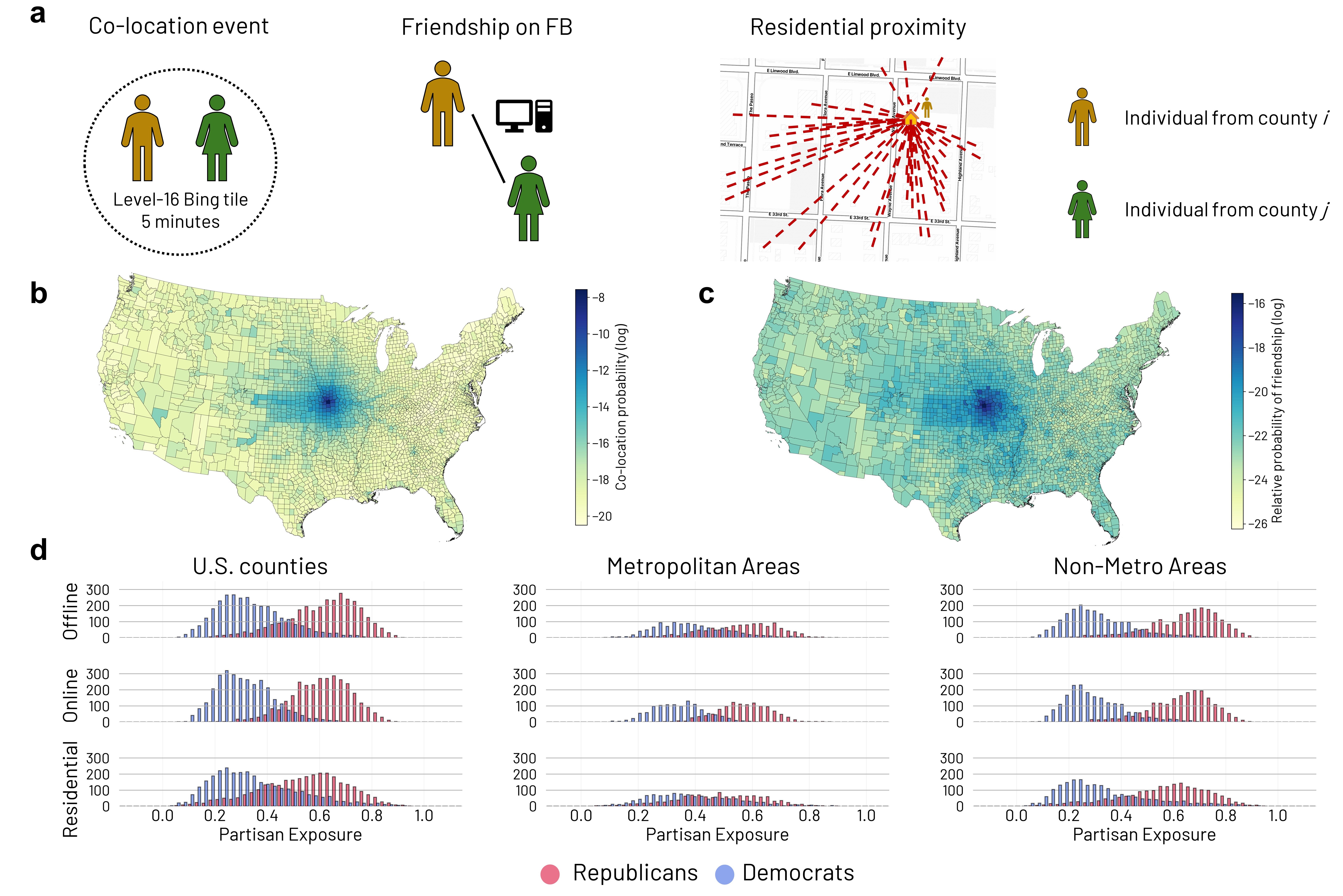
Figure 1: The three dimensions considered to estimate partisan exposure. (a) A co-location event between two randomly selected individuals from counties i and j is defined as being co-located in the same place for at least 5 minutes, while the Social Connectedness Index accounts for the number of friendships on Facebook between individuals from i and j. Residential proximity considers the nearest 1,000 individuals that registered to vote. (b and c) Co-location probabilities and relative probabilities of friendship on Facebook, respectively, between Jackson County, MO, and all the others. (d) Distributions of partisan exposure by county, including metro and non-metro areas. Note: distributions are not population-weighted.

We then compute residential partisan exposure for each county from the dataset provided by R. Enos [38, 23], which provides the conditional probabilities of being exposed to either Republican or Democratic voters for both Republicans and Democrats at the residential level, based on the proximity to the nearest 1,000 individuals who have registered to vote. To the aim of our study, we compute partisan exposure to Democratic and Republican voters for each US county, as the probability that a random individual is exposed to Republicans or Democrats. Further details can be found in the Materials and Methods Section.

To investigate the differences between partisan exposure across the three dimensions, we perform a t-test between the distributions of offline, online, and residential exposures (SI Appendix, Table S1). Note that the distributions are not population-weighted. Considering all counties in the contiguous United States (Fig. 1d), we find significant differences ($p<.001$) in partisan exposure to Republican voters when comparing residential exposure to either online or offline exposure. However, no significant difference ($p>.05$) is observed between the distributions of online and offline exposures (SI Appendix, Table S1). For Democratic voters, partisan exposure differences across the various dimensions are also significant ($p<.001$).

Additionally, we categorize counties into metropolitan and non-metro areas based on the Rural-Urban Continuum Codes (RUCC) and test the significance of the differences between partisan exposures (Fig. 1d; see also SI Appendix, Tables S2 and S3). We assess the differences between exposure in metropolitan and non-metro areas using a Welch’s t-test (SI Appendix, Table S4). Results show significant differences in the distributions of partisan exposure to Republicans in metro areas. In contrast, offline and residential exposure to Democrats shows similar patterns, with no significant differences (SI Appendix, Table S2). In non-metropolitan areas, there are significant differences ($p<.001$) between offline, online, and residential exposures to both Democrats and Republicans (SI Appendix, Table S3). Finally, we identify significant differences ($p<.001$) between exposure in metro and non-metro areas for all the dimensions (SI Appendix, Table S4).

Partisan exposure and voting behavior

We estimate the relationship between physical, online, and residential partisan exposure and voting behavior through several statistical models to assess their relative contribution to voting dynamics. As with the computation of partisan exposure, voting patterns of US counties are defined as the average share of Democratic and Republican voters in the last three presidential elections (i.e., 2012, 2016, and 2020). The shares are not complementary because we account for third-party and null votes. According to the normal vote concept [39], this method adjusts for candidate- or election-specific influences on voter turnout and election results, providing a more accurate assessment of voting patterns. In all the models, the shares of Democrats and Republicans in the US counties are our dependent or target variables.

We first model each dimension of partisan exposure ($PE$) and voting patterns for Democrats and Republicans separately with spatial autoregressive lag models [40], accounting for spatial autocorrelation across all counties in the contiguous United States. We use k-nearest neighbor to compute spatial weights, with different values of $k$ ($5$, $7$, and $10$) for robustness. Similarly, we evaluate the relationship between partisan exposure and voting patterns in metropolitan and non-metropolitan areas with ordinary least squares (OLS) regressions. Finally, we compare swing and non-swing counties, considering counties with varying political outcomes in the last three presidential elections and whose voting patterns are consequently less predictable.

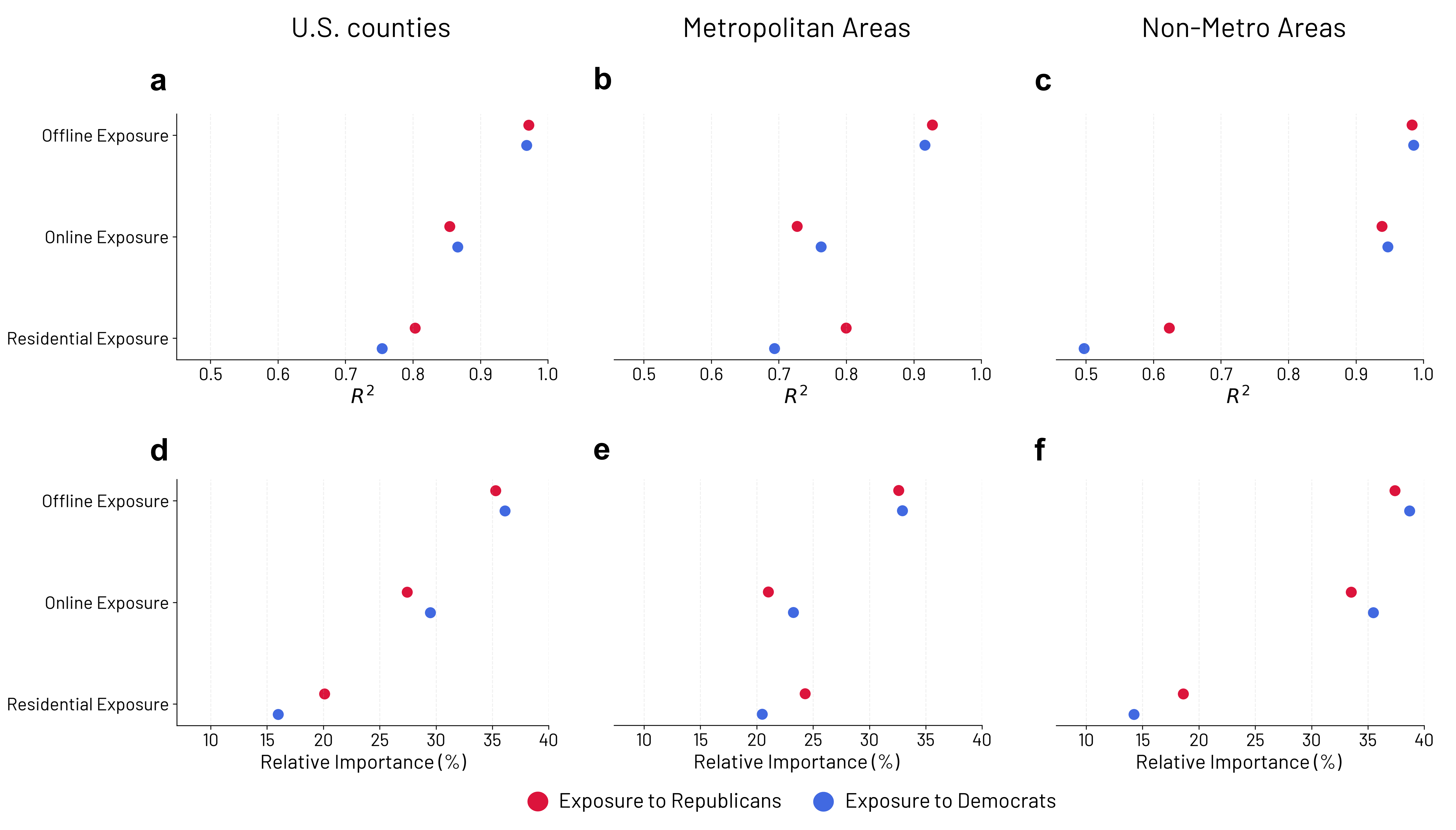
Figure 2: Relative contribution of the three dimensions of partisan exposure on voting patterns. Physical partisan exposure outweighs online and residential exposure considering all the counties in the contiguous US in both spatial models (a) with $k=7$ ($R^{2}$) and dominance analysis (d) which considers demographic and socioeconomic controls. The result is consistent in both metropolitan (b and e) and non-metro areas (c and f), employing both OLS models ($R^{2}$) and dominance analysis.

In Fig. 2, we show the results for both spatial and OLS models, for Democrats and Republicans, further disaggregated by metropolitan and non-metropolitan counties. We compare the models’ ability to explain the variance in the dependent variable using $R^{2}$, with consistent results when measuring the model’s quality with the Akaike Information Criterion (AIC) and log-likelihood. Considering all US counties and accounting for spatial autocorrelation, physical partisan exposure to both Democrats and Republicans, as captured by Colocation Maps, is the dimension that best explains the variance in the share of Democratic ($R^{2}=0.97$) and Republican ($R^{2}=0.97$) votes respectively, when compared to online ($R^{2}=0.87$ and $0.85$) and residential ($R^{2}=0.80$ and $0.75$) exposures (Fig. 2a). Moreover, when comparing online and residential partisan exposures, the former has a higher explanatory power of the variance in voting patterns than the latter, for Democrats and Republicans. Disentangling the analysis across the urban-rural axis according to the RUCC, we find that while in non-metro areas offline and online partisan exposures have similar predictive power ($R^{2}=0.98$ and $0.94$ respectively for Republicans and $R^{2}=0.99$ and $0.95$ for Democrats), in metro areas the partisan exposure captured by Colocation Maps significantly outperforms both the other dimensions, with the $R^{2}$ of the model related to offline exposure equal to $0.93$ (Republicans) and $0.92$ (Democrats) compared to online ($0.73$ and $0.76$ respectively) and residential ($0.80$ and $0.69$) exposures (Figs. 2b and 2c). Therefore, in metropolitan areas, voting patterns are predominantly associated with the partisan exposure to Democrats and Republicans in the physical space, when sharing the same social context.

To check the robustness of our results, we test our findings with different modeling approaches. First, we perform a dominance analysis [41] to compare the three dimensions, accounting for possible demographic and socioeconomic confounders, including the shares of Hispanics and Latinos, African Americans, graduated individuals, unemployment, and urban population. These characteristics are selected based on the literature on the determinants of political outcomes [42, 43, 44, 42, 45, 46] and by computing Variance Inflation Factors (VIFs) to address multicollinearity issues. We refer to the Materials and Methods Section for further details about the variable selection. From this perspective, dominance analysis allows us to deal with highly correlated variables and determine the relative importance of each predictor. Fig. 2d confirms the results obtained using the spatial lag models (Fig. 2a), with the higher relative importance of offline exposure in explaining the variance of US voting patterns. Specifically, offline exposure shows greater relative importance for both Republicans ($35.29\%$) and Democrats ($36.12\%$) compared to the online ($27.43\%$ and $29.5\%$ respectively) and residential ($20.11\%$ and $15.97\%$) exposures. Moreover, the results of the OLS models (Figs. 2b and 2c) are confirmed by the dominance analysis in both metropolitan (Fig. 2e) and non-metropolitan areas (Fig. 2f). See the SI Appendix for complete results.

Second, we enhance the generalizability of our findings by modeling the relationship between the three $PE$ dimensions and the voting patterns using the Elastic Net models with k-fold cross-validation [47] (see Materials and Methods Section and SI Appendix, Table S22). Consistently with previous results, physical exposure, as captured by Colocation Maps, has the greatest impact on the prediction compared to online and residential exposures ($\beta=1.08$ compared to $-0.18$ and $0.09$ for Republicans and $\beta=1.15$ compared to $-0.22$ and $0.06$ for Democrats). Overall, the models achieve high performances in terms of generalizability, with $R^{2}$ equal to $0.97$ in the test sets for both models.

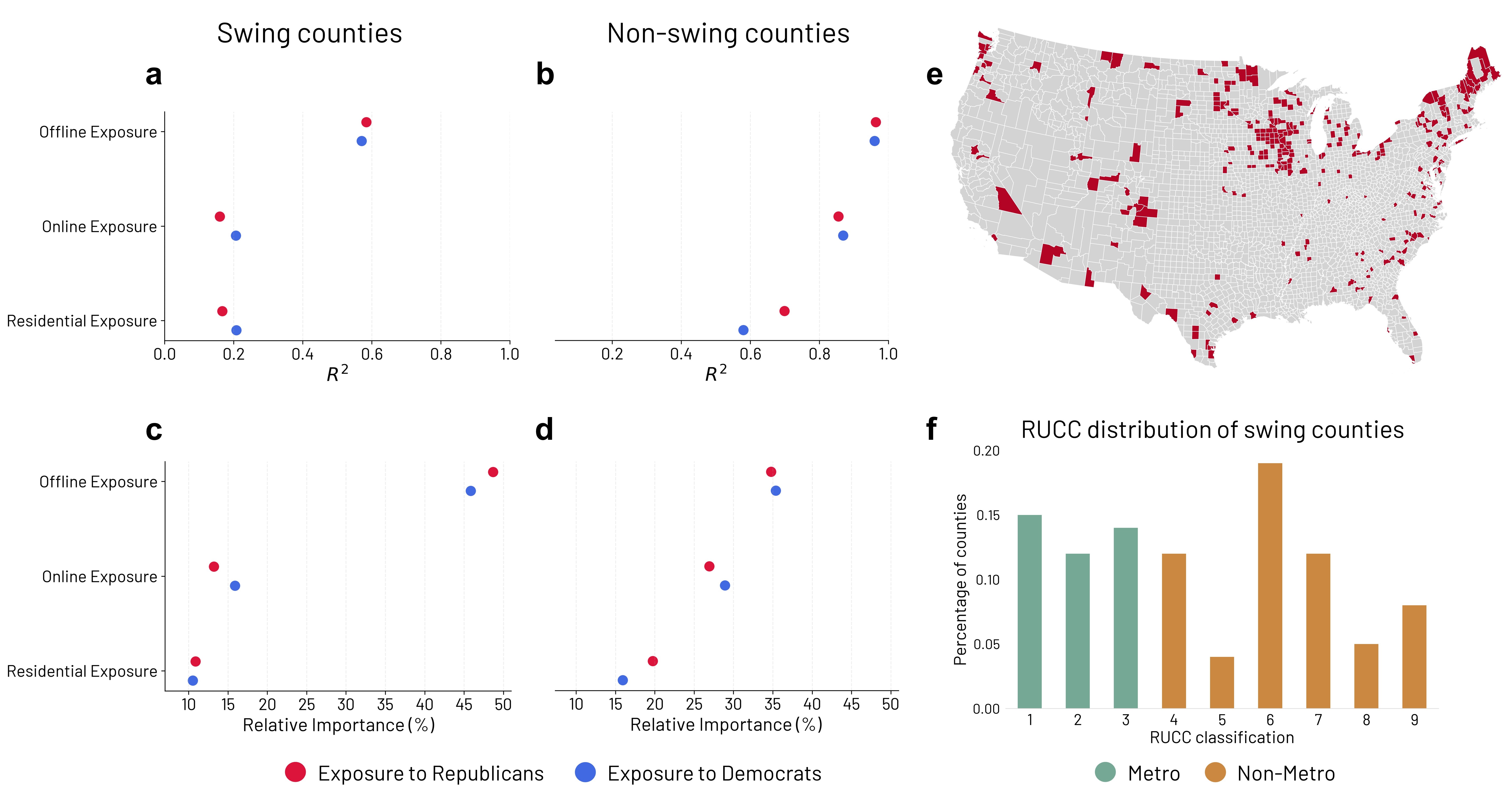
Figure 3: Relative contribution of the three dimensions of partisan exposure on voting patterns comparing swing and non-swing counties. (a and b) $R^{2}$ of the OLS models for the swing counties and non-swing counties, respectively, highlight the higher predictive power of physical exposure, especially in the swing counties. (c and d) Dominance analysis for the swing and non-swing counties, respectively, considering the three dimensions, along with demographic and socioeconomic controls. (e and f) Map of the swing counties in the contiguous US and distribution according to the RUCC classification.

We then categorize counties into swing and non-swing counties based on their voting patterns in the presidential elections from 2012 to 2020. We also consider the 2008 presidential election as an additional robustness check in the SI Appendix (Fig. S2). Swing counties are defined as counties that experienced electoral volatility, shifting their majority support among different parties across three consecutive presidential elections. We refer to the Materials and Methods Section for further details. The experienced physical exposure $PE$ to Democrats and Republicans best explains the variance in voting patterns for both swing and non-swing counties. However, when comparing swing and non-swing counties, the difference between the predictive power of physical and online exposures is larger in the swing counties in both OLS models and dominance analysis. Specifically, in the OLS models for Republicans and Democrats, physical exposure in swing counties explains $58\%$ and $57\%$ of the variance, respectively, while online exposure accounts for only $16\%$ and $21\%$ of the variance, respectively (Fig. 3a and SI Appendix, Tables S10 and S18). In contrast, in non-swing counties, the differences between offline and online predictive power are reduced to $11\%$ in the model for the Republican vote and $9\%$ in the model for the Democratic vote (Fig. 3c and SI Appendix, Tables S11 and S19). Therefore, voting patterns are strongly associated with partisan exposure in the physical space, demonstrating a greater influence than online connections and residential proximity.

Finally, as a sensitivity analysis, we excluded the self-loops from the co-location and online connections networks. A self-loop represents the co-location or friendship probability between individuals in county $i$ and residents of the same county, leading to an edge between $i$ and itself. In the physical network, local exposure represents a substantial and fundamental aspect of an individual’s exposure, with a median value of counties’ extroversion equal to $0.27$. Conversely, while local exposure still plays a significant role in the online network, the network structure is more heterogeneous and characterized by higher external exposure (median value of extroversion equal to $1.19$). Detailed descriptions can be found in the SI Appendix (Fig. S3). Fig. S4 of the SI Appendix shows that when local exposure is excluded from the computation of $PE$, online ties outweigh physical proximity in predicting US political outcomes at the county level. Specifically, considering all the US counties, online exposure explains $65\%$ and $67\%$ ($R^{2}$) of the variance of voting patterns for Republicans and Democrats, respectively, compared to $61\%$ and $60\%$ explained by the physical proximity (Fig. S4a). However, predictive performances are lower when local exposure is not considered, particularly in the offline network, characterized by low heterogeneity and extroversion. Hence, local exposure appears to be a fundamental dimension in predicting voting outcomes.

Partisan segregation across demographic and socioeconomic factors

To investigate the levels of social segregation across political lines in the US, we estimate partisan segregation for each dimension as the net difference between exposure to Republicans and exposure to Democrats in a given county. The metric is scaled from 0 (indicating exclusive exposure to Democrats) to 1 (indicating exclusive exposure to Republicans). Intermediate values represent different mixing levels, with 0.5 indicating an equal share of exposure between the two electorates (see Materials and Methods Section for further details). We then investigate the relationship between partisan segregation and the county demographic and socioeconomic characteristics, focusing on metropolitan areas. To this aim, we predict partisan segregation for each network dimension using Gradient Boosting (GB) regressions, based on a set of demographic and socioeconomic factors: the shares of Hispanics and Latinos, African Americans, graduated individuals, unemployment, and urban population. Additionally, we enhance model explainability by computing SHAP values [48], which provide importance scores that represent the impact of each variable on the predicted outcome. We refer to the Materials and Methods for further details on machine learning models.

We perform Welch’s t-tests to assess differences between physical, online, and residential partisan segregation, revealing significant differences ($p<.001$) between them (see SI Appendix, Table S23). Overall, partisan segregation in the physical world, both considering co-location maps and residential sorting, is higher than online segregation. As shown by the distributions of Fig. 4, in the offline and the residential networks we observe more frequently counties characterized by $PS>0.75$ (highly Republican-segregated) or $PS<0.25$ (highly Democrat-segregated). In particular, largely populated urban areas display values of $PS<0.2$ in the offline networks, that are not met by the online ties.

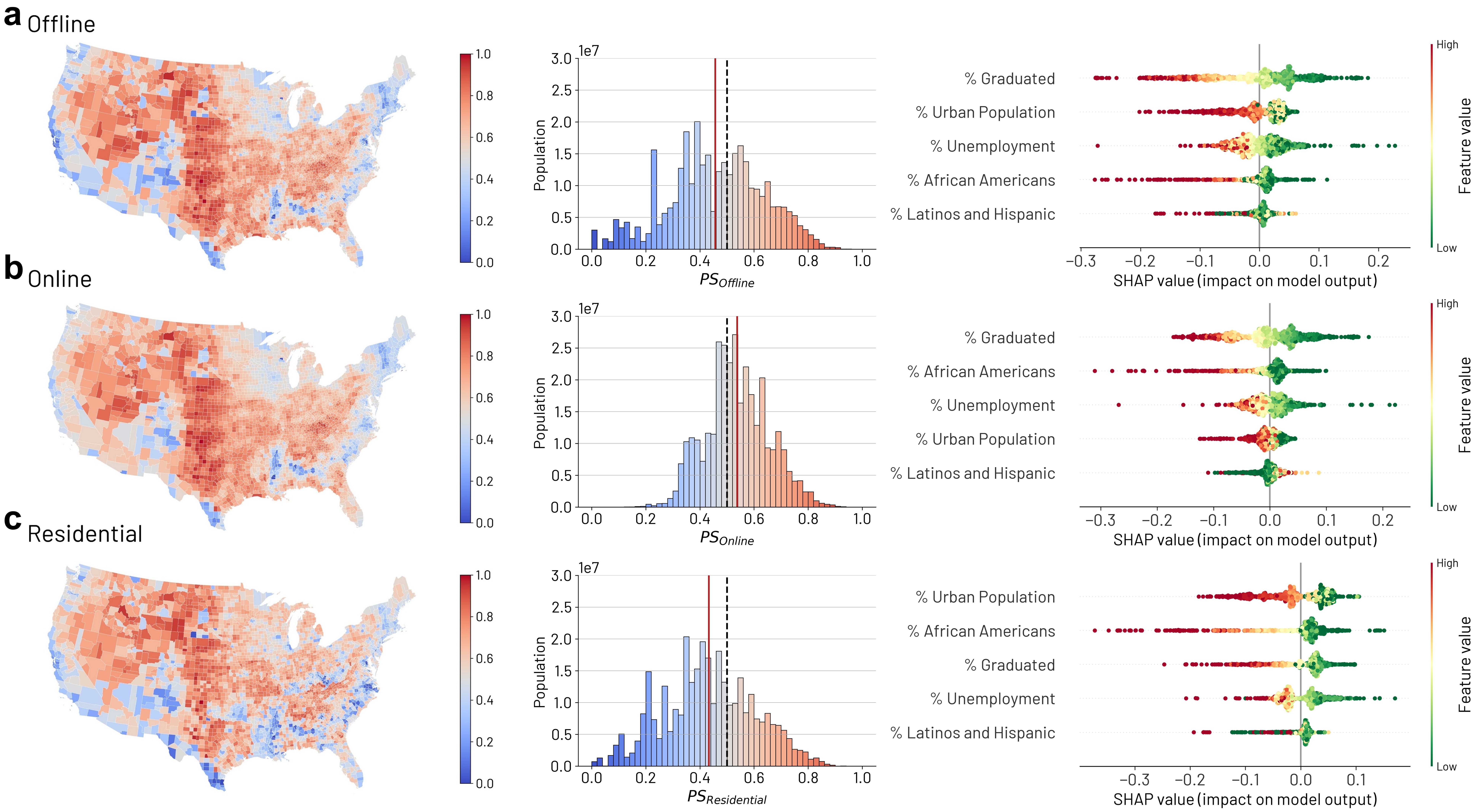
Figure 4: Partisan segregation across demographic and socioeconomic factors for each dimension. Maps and population-weighted distributions of the partisan segregation as captured by the Colocation Maps (a), Social Connectedness Index (b), and at the residential level (c). The red solid line represents the weighted average, while the black dashed line indicates balanced social mixing ($0.5$). For each dimension, the SHAP values distributions, computed from the GB regressions, highlight how the demographic and socioeconomic characteristics of the counties impact partisan segregation. Predictors are ordered by their impact on the final prediction, with points colored red for high and green for low values.

Overall, GB regressions effectively explain the variance of offline ($R^{2}=0.63$), online ($0.55$), and residential ($0.64$) segregation. Moreover, Fig. 4 shows the distribution of the SHAP values for each predictor related to offline, online, and residential partisan segregation in metropolitan areas. Predictors are ordered based on the impact on the prediction, with the most impactful variable at the top, and each point represents an observation. Finally, each point is colored based on its value, with red indicating high values and green indicating low values.

The share of graduated individuals is the best predictor for both partisan segregations computed from offline (average absolute impact equal to $0.06$) and online ($0.048$) networks. While counties with higher shares of graduated individuals tend to be exposed to Democrats (with higher Democratic segregation), counties with less educated individuals tend to be co-located and connected online with individuals who vote for the Republican party (Figs. 4a and 4b). In contrast, at the residential level, the educational level follows similar patterns but is the third predictor (mean average impact equal to $0.038$) in terms of variable importance (Fig. 4c).

Moreover, we find that the shares of urban population have a greater impact on partisan segregation in offline spaces, including both co-location ($0.033$) and residential ($0.045$) exposures, compared to online connections ($0.016$). Specifically, metropolitan areas with urban characteristics show higher levels of Democratic segregation in offline spaces (Fig. 4).

Furthermore, partisan segregation is closely tied to the presence of ethnic communities. Specifically, the presence of a large share of African Americans is the second most relevant predictor for partisan segregation both online ($0.026$) and at the residential level ($0.042$) in metropolitan areas. Large communities of African Americans are associated with predominant exposure to Democrats, while areas with low African American presence tend to Republican segregation (Fig. 4). Finally, as shown in Fig. 4, the presence of Latinos and Hispanics is the least relevant predictor in all the dimensions, namely offline ($0.014$), online ($0.012$), and at the residential level ($0.016$). Interestingly, a larger share of Latinos and Hispanics in US counties are associated with higher levels of Democratic and Republican offline and online segregation.

Discussion

In this study, we compared partisan exposure across physical and online spaces, investigated the relationship between partisan exposure and the voting patterns of US counties, and evaluated the association between partisan segregation in online and physical spaces and the underlying counties’ demographic and socioeconomic characteristics. Our findings highlight the dominant role of physical proximity and local exposure in predicting voting patterns in the United States, outperforming the influence of online ties and residential proximity. The result was consistent across both metropolitan and non-metro areas, as well as in swing and non-swing counties. Moreover, we found that partisan segregation is higher in offline social networks than online ones, and such difference is primarily driven by individuals’ educational attainment. The urban-rural divide significantly shapes offline and residential partisan segregation, with Republican voter segregation more prevalent in metro areas with large rural populations. Thus, physical partisan exposure, which is the best predictor of voting outcomes, is also strongly associated with educational attainment and urbanization levels.

Our findings contribute to a better understanding of the relationship between social networks, physical and online spaces, and political behavior. Previous studies have mainly focused on the impact of new media technologies, particularly online social media, on affective polarization and political elections [5, 6, 7, 8, 9, 10, 11, 12, 13], either through mechanisms of echo chambers and selective exposure [6, 49] or through interactions outside one’s local bubbles [11]. In this context, our study, by comparing physical and online networks, highlights the high relevance of physical space and offline ties in predicting political voting patterns at the county level, in both metro and non-metro areas, and especially where political voting is less predictable (i.e., swing counties). Local exposure and physical proximity, characterized by low heterogeneity of social exposure and low extroversion, not only account for social ties but also for visitation patterns to places where individuals spend their time, as captured by the co-location probabilities. Our findings call for a deeper investigation of geographic space, human behavior, and the social groups that share this space, which often tend to share beliefs and opinions through mechanisms of homophily [50].

Moreover, partisan exposure and segregation vary across physical and online spaces, as well as between urban and rural areas. In line with the literature, our findings highlight that a large share of the US population, up to 10%, has low exposure to outgroup partisans, not only in the residential sphere [23], but also in physical social encounters, where experienced segregation is even greater than online partisan segregation. Both forms of experienced segregation are associated with individuals’ educational attainment, a known driver of socioeconomic segregation [51]. Furthermore, the tendency of Republican voter segregation in areas with large rural populations reveals differences between urban and rural areas related not only in terms of political party support [52] but also in partisan exposure [23]. In contrast, consistent with the literature, our findings show greater Democratic segregation in high-density urban areas [23]. These findings are relevant for public policy as they highlight how human activities, either online or in physical social encounters, reduce political social mixing, driven by educational and geographic disparities. Addressing these underlying factors can help policymakers to reduce social divisions and enhance social cohesion.

Our study comes with some limitations. First, we compared online and physical networks using aggregated observational data from social media platforms. Despite the two-step reweighting applied to the Colocation Maps dataset [37], Facebook data might under-represent certain categories of people (e.g., young and older individuals) and the population of rural areas [53]. Moreover, these aggregated networks are considered at a rather coarse geographical level, the US county, whose population sizes vary widely, ranging from $83$ individuals (Loving County, TX) to over $10$ million inhabitants. Furthermore, we use the SCI as a proxy of online connections, but people interact through multiple social media platforms and have access to novel information from different sources. However, although some studies have attempted to map online interactions spatially [27, 54, 55], achieving comprehensive coverage across the entire US remains challenging. Finally, we acknowledge that co-location does not imply a face-to-face interaction between individuals. However, co-presence temporal networks have been found to have comparable structural and statistical features to face-to-face interaction temporal networks [56].

Overall, our study underscores the centrality of physical space in understanding human and political behavior in both urban and rural areas. Despite challenges related to data limitations and privacy concerns, future studies on political polarization, partisan segregation, and their impact on political outcomes should not overlook the importance of real-world interactions in the physical space.

Materials and methods

Data sources

Online network

We use the Social Connectedness Index (SCI) [33] dataset provided by Meta through its Data for Good program as a proxy of online connections. The SCI measures the social connectedness between administrative areas by computing the probability at which two random individuals, living respectively in administrative areas $i$ and $j$, are friends on Facebook, as of April 2016 [33]. The SCI is available at both the county and zip code levels. We analyze online connections at the county level to enable comparison with the Colocation Maps. Specifically, to be able to compare the online probabilities with the offline ones, we use the original version of the dataset adopted in Bailey et al. [33], which includes the relative probabilities of friendship between counties computed as follows:

$$rel\_prob\_friend=C\frac{sci}{pop_{i}*pop_{j}},$$ (1)

where $sci$ is the number of Facebook friendships between administrative regions $i$ and $j$ and $pop_{i}$ and $pop_{j}$ are the population size of $i$ and $j$. $C$ is a scaling factor, equal to $10^{12}$, that we drop to obtain the raw probabilities.

Offline network

We use the Colocation Maps [37] provided by Meta through its Data for Good program to measure offline exposure. Similarly to the SCI, the dataset provides the weekly co-location probability between two randomly selected individuals from two administrative areas $i$ and $j$. A co-location event (Fig. 1a) is registered when two individuals who enabled location-based services on the Facebook smartphone application are located in the same place (i.e., a level-16 Bing-tile, approximately 600 by 600 meters at the equator) at the same time for at least 5 minutes. The co-location probability between geographic regions $i$ and $j$ is then determined by the number of co-location events between individuals from $i$ and $j$ weighted by their population sizes. As described by Iyer et al. [37], the authors applied a two-steps reweighting to enhance representativeness. Specifically, the first step aligns the Facebook user data to the general population, and the second step reweights the Colocation Maps population to the Facebook user base. The dataset has been designed and used mainly for epidemiological purposes [57, 58]. For the aim of our study, we collected weekly co-location probabilities between US counties from August 2022 to January 2024, for a total of $76$ weeks/observations. We then use the average co-location value over the full period to mitigate seasonality effects and data sparsity and reduce computational errors in data measurement, ensuring a more realistic measure of physical exposure between counties.

Residential partisan exposure

We compare online and offline networks with a measure of residential proximity, based on individuals’ residential locations. To this purpose, we use the dataset provided by R. Enos [38] supporting the recent study by Brown et al. [23], which includes the conditional probability of exposure to Democratic and Republican voters, conditioned on an individual’s political affiliation (either Democrat or Republican). The probabilities are computed based on the nearest 1,000 individuals, but the results remain consistent even considering a larger sample size of 50,000 individuals. The dataset is derived from voter registration records, which require individuals in the majority of US states to declare their party affiliation and it provides information at different geographical levels. To have a measure of partisan exposure at the residential level, we compute the probabilities of exposure to Democrats and Republicans for a random individual for each US county. Specifically, from the available raw data, we compute the partisan exposure to Republicans for a county $i$ as follows:

$$P(R)=\frac{P(R|D)P(D)}{P(D|R)},$$ (2)

where $P(R|D)$ is the conditional probability of exposure to Republicans being a Democrat and $P(D|R)$ is the conditional probability of exposure to Democrats being a Republican. Similarly, we compute the partisan exposure to Democrats.

Voting patterns in US counties

We define the voting patterns of the counties in the contiguous United States following the normal vote concept [39] to account for candidate- and election-specific influences on voting outcomes. Specifically, the share of Republican and Democratic voters for each county is computed as the average of the last three presidential elections (i.e., 2012, 2016, and 2020). We obtained data on presidential election results from the work conducted by Algara and Amlani [59].

Demographic and socioeconomic indicators

To evaluate the relationship between partisan segregation and county characteristics, we obtain data from the 2017-2021 5-year estimates of the American Community Survey (ACS) provided by the United States Census Bureau [60]. Specifically, we use data related to the shares of Hispanics and Latinos, African Americans, unemployed individuals, and urban population. Moreover, we use the information about the share of graduated individuals for each county provided by Chetty et al. [61] through the Opportunity Insights repository [62]. We select this information from a broader set of counties’ characteristics by computing Variance Inflation Factors (VIFs) to address multicollinearity issues (See SI for further details) and drawing on the literature on the determinants of county outcomes in US presidential elections. Specifically, ethnicity is one of the strongest predictors of political outcomes, with African Americans tending to vote for the Democratic party [42, 46]. Additionally, educational attainment, which is highly correlated with income (addressed through VIF), is associated with Democratic voting tendencies [42, 44]. Finally, unemployment is one of the economic indicators that impact political outcomes [45], as well as the urban-rural characteristics and divide [43, 52].

Metropolitan and Non-Metropolitan areas

We define metropolitan and non-metropolitan areas based on the Rural-Urban Continuum Codes (RUCC) 2013 [63]. Specifically, metropolitan areas include the codes 1 to 3 (RUCC 1–3), while non-metropolitan areas include codes 4 to 9 (RUCC 4–9).

Methods

Partisan exposure

We define partisan exposure of a county $i$ as the relative exposure to people with a certain voting behavior (i.e., Republican or Democratic voters), weighted by either the co-location probability between counties $i$ and $j$ (i.e., Colocation Maps) or the relative probability of friendship on Facebook between $i$ and $j$ (i.e., the Social Connectedness Index). Formally, we define the partisan exposure as:

$$PE_{p}(i)=\sum^{N}_{j}\ v_{p}(j)\ \frac{p_{ij}}{\sum^{N}_{k}p_{ik}}\,,$$ (3)

where $PE_{p}(i)$ is the partisan exposure to either Republicans or Democrats for a county $i$, $N$ is the number of US counties, $v_{p}(j)$ is the percentage of Republican or Democratic voters in the county $j$, and $p_{ij}$ is either the co-location probability between counties $i$ and $j$, or the relative probability of friendship on Facebook between $i$ and $j$. Partisan exposure ranges from 0 (low exposure to either Democrats or Republicans) to 1 (high exposure to either Democrats or Republicans). The sum of partisan exposures to Republicans and Democrats is less than $1$ because we account for null and third-party votes.

Residential and experienced partisan segregation

Residential and experienced partisan segregation are computed from the residential and either online or offline partisan exposures respectively. Specifically, partisan segregation is computed as the difference between exposure to Republicans and to Democrats. The index is scaled from 0 (indicating exclusive exposure to Democrats) to 1 (indicating exclusive exposure to Republicans). Intermediate values indicate varying levels of partisan mixing. The index is computed as follows:

$$PS(i)=PE_{rep}(i)-PE_{dem}(i),$$ (4)

where $PS(i)$ is the index of partisan segregation for a county $i$, $PE_{rep}(i)$ is the partisan exposure to Republicans and $PE_{dem}(i)$ is the partisan exposure to Democrats.

Swing counties

We define swing counties as counties that experienced different majority outcomes in consecutive presidential elections between 2012 and 2020 (for example, a majority of Republican votes in 2012 followed by a majority of votes for the Democratic candidate in 2016). The number of swing counties according to our definition is $285$. Hence, swing counties can determine political elections with their results. Figs. 3e and 3f show their geographic locations and classification according to the RUCC. Swing counties, as defined in our study, are located in both metropolitan and non-metropolitan areas, mainly concentrated in the Midwest and Northeast regions. We also perform the same analyses defining swing counties as counties that experienced different outcomes between 2008 and 2020, for a total of $455$ counties (see SI Appendix, Fig. S2).

Spatial Autoregressive Lag Models and OLS

To explore which dimension of partisan exposure better predicts voting patterns in US counties, we separately model physical, online, and residential exposures using spatial regressions, both for Republicans and Democrats. Due to the high correlation between these dimensions, combining them in the same model could impact the interpretation and potentially lead to misleading conclusions. Specifically, we use spatial lag models [40], which are autoregressive models that account for spatial autocorrelation among observations. Specifically, the models are defined as:

$$v_{p}(i)=\alpha+\rho Wy+\beta PE_{p,d}(i)+\epsilon,$$ (5)

where $v$ is the share of either Republican or Democratic votes, $p$ is either Democrats or Republicans, $\rho Wy$ is the autoregressive coefficient, and $PE$ is the partisan exposure to either Democrats or Republicans, $p$. The model is fitted for each dimension $d$, namely offline, online, and residential. To enhance the robustness of the method, we compute k-nearest neighbour spatial weights $W$ using different values of $k$, specifically $5$, $7$, and $10$. This approach is preferred because contiguity-based methods would exclude non-contiguous counties from the analysis. When comparing metropolitan and non-metropolitan areas based on the Rural-Urban Continuum Codes (RUCC), we use ordinary least squares (OLS) regressions. In both types of models, we determine the dimension that better predicts voting patterns based on its ability to explain the variance of the dependent variable (i.e., $R^{2}$).

Dominance analysis

While we treat the three dimensions separately in the regressions, due to their high collinearity, we use dominance analysis [41] to consider them together and evaluate their relative importance. This method allows us to evaluate the impact of predictors by measuring the contribution of each predictor through designing a series of linear regressions with all possible combinations of predictors to systematically assess and compare each variable’s individual and combined predictive power. Specifically, we perform dominance analysis for both the exposure to Republicans and Democrats, including in the models physical, online, and residential exposure along with the demographic and socioeconomic characteristics previously described. The method provides the relative importance of each predictor as a percentage (Fig. 2). The full model is defined as:

$$v_{p}(i)=\alpha+\beta_{1}PE_{p,offline}(i)+\beta_{2}PE_{p,online}(i)+\beta_{3}PE_{p,residential}(i)+\beta_{n}controls(i)+\epsilon,$$ (6)

where we also account for the demographic and socioeconomic characteristics of the counties.

Predictive modeling and model explainability

To enhance the robustness and the generalizability of the result related to the relationship between partisan exposure and voting patterns, we model each dimension separately using Elastic Net [47] models with k-fold cross-validation ($k=5$). This allows us to evaluate beta coefficients of the model using a regularization technique.

Second, we predict partisan segregation in metropolitan areas (RUCC 1–3) for each dimension using demographic and socioeconomic characteristics of the US counties. To this aim, we model Gradient Boosting regressions and compute SHAP [48] values to interpret the predictions. Specifically, drawing on game theory, the SHAP framework computes importance scores for each predictor, representing the impact of each variable on the final prediction. Before training the model, we split the dataset into training and test sets using a 70/30 ratio.

Data and code availability

Colocation Maps are available through the Meta Data for Good program by signing a data sharing agreement (https://dataforgood.facebook.com/). The Social Connectedness Index (SCI) is publicly available through the Humanitarian Data Exchange portal (https://data.humdata.org/dataset/social-connectedness-index). Residential partisan exposure is available through the Harvard Dataverse (https://doi.org/10.7910/DVN/A40X5L). The code to reproduce the study’s findings is available at https://github.com/tonmarco.

Author contribution statement

M.To. collected and analyzed the data, performed the research, and drafted the first version of the manuscript. M.To., B.L., M.Ti. designed the study, interpreted the results, provided critical feedback, helped shape the manuscript, and revised it. All authors approved the final version of the manuscript.

References

- [1] Baldassarri, D. & Gelman, A. Partisans without constraint: Political polarization and trends in american public opinion. \JournalTitleAmerican Journal of Sociology 114, 408–446 (2008).
- [2] Iyengar, S., Sood, G. & Lelkes, Y. Affect, not ideology: A social identity perspective on polarization. \JournalTitlePublic opinion quarterly 76, 405–431 (2012).
- [3] Webster, S. W. & Abramowitz, A. I. The ideological foundations of affective polarization in the us electorate. \JournalTitleAmerican Politics Research 45, 621–647 (2017).
- [4] Iyengar, S., Lelkes, Y., Levendusky, M., Malhotra, N. & Westwood, S. J. The origins and consequences of affective polarization in the united states. \JournalTitleAnnual review of political science 22, 129–146 (2019).
- [5] Bessi, A. & Ferrara, E. Social bots distort the 2016 us presidential election online discussion. \JournalTitleFirst monday 21 (2016).
- [6] Del Vicario, M. et al. The spreading of misinformation online. \JournalTitleProceedings of the national academy of Sciences 113, 554–559 (2016).
- [7] Allcott, H. & Gentzkow, M. Social media and fake news in the 2016 election. \JournalTitleJournal of economic perspectives 31, 211–236 (2017).
- [8] Badawy, A., Ferrara, E. & Lerman, K. Analyzing the digital traces of political manipulation: The 2016 russian interference twitter campaign. In 2018 IEEE/ACM international conference on advances in social networks analysis and mining (ASONAM), 258–265 (IEEE, 2018).
- [9] Boxell, L., Gentzkow, M. & Shapiro, J. M. Greater internet use is not associated with faster growth in political polarization among us demographic groups. \JournalTitleProceedings of the National Academy of Sciences 114, 10612–10617 (2017).
- [10] Lazer, D. M. et al. The science of fake news. \JournalTitleScience 359, 1094–1096 (2018).
- [11] Törnberg, P. How digital media drive affective polarization through partisan sorting. \JournalTitleProceedings of the National Academy of Sciences 119, e2207159119 (2022).
- [12] Muise, D. et al. Quantifying partisan news diets in web and tv audiences. \JournalTitleScience advances 8, eabn0083 (2022).
- [13] Allcott, H. et al. The effects of facebook and instagram on the 2020 election: A deactivation experiment. \JournalTitleProceedings of the National Academy of Sciences 121, e2321584121 (2024).
- [14] Eagle, N., Macy, M. & Claxton, R. Network diversity and economic development. \JournalTitleScience 328, 1029–1031 (2010).
- [15] Chetty, R. et al. Social capital i: measurement and associations with economic mobility. \JournalTitleNature 608, 108–121 (2022).
- [16] Chetty, R. et al. Social capital ii: determinants of economic connectedness. \JournalTitleNature 608, 122–134 (2022).
- [17] Charles, C. Z. The dynamics of racial residential segregation. \JournalTitleAnnual review of sociology 29, 167–207 (2003).
- [18] Reardon, S. F. & Bischoff, K. Income inequality and income segregation. \JournalTitleAmerican journal of sociology 116, 1092–1153 (2011).
- [19] Moro, E., Calacci, D., Dong, X. & Pentland, A. Mobility patterns are associated with experienced income segregation in large us cities. \JournalTitleNature communications 12, 4633 (2021).
- [20] Bishop, B. & Cushing, R. G. The big sort: Why the clustering of like-minded America is tearing us apart (Houghton Mifflin Harcourt, 2009).
- [21] Gimpel, J. G. & Hui, I. S. Seeking politically compatible neighbors? the role of neighborhood partisan composition in residential sorting. \JournalTitlePolitical Geography 48, 130–142 (2015).
- [22] Mummolo, J. & Nall, C. Why partisans do not sort: The constraints on political segregation. \JournalTitleThe Journal of Politics 79, 45–59 (2017).
- [23] Brown, J. R. & Enos, R. D. The measurement of partisan sorting for 180 million voters. \JournalTitleNature Human Behaviour 5, 998–1008 (2021).
- [24] Wang, Q., Phillips, N. E., Small, M. L. & Sampson, R. J. Urban mobility and neighborhood isolation in america’s 50 largest cities. \JournalTitleProceedings of the National Academy of Sciences 115, 7735–7740 (2018).
- [25] Zhang, Y., Cheng, S., Li, Z. & Jiang, W. Human mobility patterns are associated with experienced partisan segregation in us metropolitan areas. \JournalTitleScientific Reports 13, 9768 (2023).
- [26] de la Prada, À. G. & Small, M. L. How people are exposed to neighborhoods racially different from their own. \JournalTitleProceedings of the National Academy of Sciences 121, e2401661121 (2024).
- [27] Dong, X. et al. Segregated interactions in urban and online space. \JournalTitleEPJ Data Science 9, 20 (2020).
- [28] Granovetter, M. S. The strength of weak ties. \JournalTitleAmerican journal of sociology 78, 1360–1380 (1973).
- [29] Aral, S. & Van Alstyne, M. The diversity-bandwidth trade-off. \JournalTitleAmerican journal of sociology 117, 90–171 (2011).
- [30] Park, P. S., Blumenstock, J. E. & Macy, M. W. The strength of long-range ties in population-scale social networks. \JournalTitleScience 362, 1410–1413 (2018).
- [31] Granovetter, M. Economic action and social structure: The problem of embeddedness. \JournalTitleAmerican journal of sociology 91, 481–510 (1985).
- [32] Jahani, E., Fraiberger, S. P., Bailey, M. & Eckles, D. Long ties, disruptive life events, and economic prosperity. \JournalTitleProceedings of the National Academy of Sciences 120, e2211062120 (2023).
- [33] Bailey, M., Cao, R., Kuchler, T., Stroebel, J. & Wong, A. Social connectedness: Measurement, determinants, and effects. \JournalTitleJournal of Economic Perspectives 32, 259–280 (2018).
- [34] Bailey, M. et al. The determinants of social connectedness in europe. In Social Informatics: 12th International Conference, SocInfo 2020, Pisa, Italy, October 6–9, 2020, Proceedings 12, 1–14 (Springer, 2020).
- [35] Nickerson, D. W. Is voting contagious? evidence from two field experiments. \JournalTitleAmerican political Science review 102, 49–57 (2008).
- [36] Braha, D. & De Aguiar, M. A. Voting contagion: Modeling and analysis of a century of us presidential elections. \JournalTitlePloS one 12, e0177970 (2017).
- [37] Iyer, S. et al. Large-scale measurement of aggregate human colocation patterns for epidemiological modeling. \JournalTitleEpidemics 100663 (2023).
- [38] Enos, R. Replication Data for: The Measurement of Partisan Sorting for 180 Million Voters, DOI: 10.7910/DVN/A40X5L (2020). Accessed: 2024-06-26.
- [39] Converse, P. E. The concept of a normal vote. \JournalTitleElections and the political order 9, 39 (1966).
- [40] Anselin, L. Spatial Econometrics: Methods and Models (Kluwer Academic Publishers, Dordrecht, 1988).
- [41] Azen, R. & Budescu, D. V. The dominance analysis approach for comparing predictors in multiple regression. \JournalTitlePsychological methods 8, 129 (2003).
- [42] Gelman, A. & Park, D. (eds.) Red state, blue state, rich state, poor state: why Americans vote the way they do (Princeton Univ. Press, Princeton, NJ, 2010), expand. ed edn.
- [43] Scala, D. J. & Johnson, K. M. Political polarization along the rural-urban continuum? the geography of the presidential vote, 2000–2016. \JournalTitleThe ANNALS of the American Academy of Political and Social Science 672, 162–184 (2017).
- [44] Ambrosius, J. D. Blue city… red city? a comparison of competing theories of core county outcomes in us presidential elections, 2000–2012. \JournalTitleJournal of Urban Affairs 38, 169–195 (2016).
- [45] Kahane, L. H. Determinants of county-level voting patterns in the 2012 and 2016 presidential elections. \JournalTitleApplied Economics 52, 3574–3587 (2020).
- [46] Kuriwaki, S., Ansolabehere, S., Dagonel, A. & Yamauchi, S. The geography of racially polarized voting: calibrating surveys at the district level. \JournalTitleAmerican Political Science Review 118, 922–939 (2024).
- [47] Zou, H. & Hastie, T. Regularization and variable selection via the elastic net. \JournalTitleJournal of the Royal Statistical Society Series B: Statistical Methodology 67, 301–320 (2005).
- [48] Lundberg, S. M. & Lee, S.-I. A unified approach to interpreting model predictions. \JournalTitleAdvances in neural information processing systems 30 (2017).
- [49] Cinelli, M., De Francisci Morales, G., Galeazzi, A., Quattrociocchi, W. & Starnini, M. The echo chamber effect on social media. \JournalTitleProceedings of the National Academy of Sciences 118, e2023301118 (2021).
- [50] McPherson, M., Smith-Lovin, L. & Cook, J. M. Birds of a feather: Homophily in social networks. \JournalTitleAnnual review of sociology 27, 415–444 (2001).
- [51] Browning, C. R., Calder, C. A., Krivo, L. J., Smith, A. L. & Boettner, B. Socioeconomic segregation of activity spaces in urban neighborhoods: Does shared residence mean shared routines? \JournalTitleRSF: The Russell Sage Foundation Journal of the Social Sciences 3, 210–231 (2017).
- [52] Gimpel, J. G., Lovin, N., Moy, B. & Reeves, A. The urban–rural gulf in american political behavior. \JournalTitlePolitical behavior 42, 1343–1368 (2020).
- [53] Rama, D., Mejova, Y., Tizzoni, M., Kalimeri, K. & Weber, I. Facebook ads as a demographic tool to measure the urban-rural divide. In Proceedings of The Web Conference 2020, 327–338 (2020).
- [54] Morales, A. J., Dong, X., Bar-Yam, Y. & ‘Sandy’Pentland, A. Segregation and polarization in urban areas. \JournalTitleRoyal Society Open Science 6, 190573 (2019).
- [55] Tizzoni, M., Sun, K., Benusiglio, D., Karsai, M. & Perra, N. The scaling of human contacts and epidemic processes in metapopulation networks. \JournalTitleScientific reports 5, 15111 (2015).
- [56] Génois, M. & Barrat, A. Can co-location be used as a proxy for face-to-face contacts? \JournalTitleEPJ Data Science 7, 1–18 (2018).
- [57] Fritz, C. & Kauermann, G. On the interplay of regional mobility, social connectedness and the spread of covid-19 in germany. \JournalTitleJournal of the Royal Statistical Society Series A: Statistics in Society 185, 400–424 (2022).
- [58] Delussu, F., Tizzoni, M. & Gauvin, L. The limits of human mobility traces to predict the spread of COVID-19: A transfer entropy approach. \JournalTitlePNAS Nexus 2, pgad302 (2023).
- [59] Algara, C. & Amlani, S. Replication Data for: Partisanship & Nationalization in American Elections: Evidence from Presidential, Senatorial, & Gubernatorial Elections in the U.S. Counties, 1872-2020 (2021).
- [60] U.S. Census Bureau. 2021 American Community Survey 5-Year Data (2022). https://www.census.gov/programs-surveys/acs. Accessed: 2024-06-26.
- [61] Chetty, R., Friedman, J. N., Hendren, N., Jones, M. R. & Porter, S. R. The opportunity atlas: Mapping the childhood roots of social mobility. Tech. Rep., National Bureau of Economic Research (2018).
- [62] Opportunity Insights. Neighborhood Characteristics by County (2018). https://opportunityinsights.org/data. Accessed: 2024-06-26.
- [63] Rural-Urban Continuum Codes. 2013 Rural-Urban Continuum Codes (2013). https://www.ers.usda.gov/data-products/rural-urban-continuum-codes. Accessed: 2024-06-26.