A Multimodal Transformer for Live Streaming Highlight Prediction

Abstract

Recently, live streaming platforms have gained immense popularity. Traditional video highlight detection mainly focuses on visual features and utilizes both past and future content for prediction. However, live streaming requires models to infer without future frames and process complex multimodal interactions, including images, audio and text comments. To address these issues, we propose a multimodal transformer that incorporates historical look-back windows. We introduce a novel Modality Temporal Alignment Module to handle the temporal shift of cross-modal signals. Additionally, using existing datasets with limited manual annotations is insufficient for live streaming whose topics are constantly updated and changed. Therefore, we propose a novel Border-aware Pairwise Loss to learn from a large-scale dataset and utilize user implicit feedback as a weak supervision signal. Extensive experiments show our model outperforms various strong baselines on both real-world scenarios and public datasets. And we will release our dataset and code to better assess this topic.

I Introduction

Live streaming platforms represent a new type of online interaction and have experienced rapid growth in recent years. This new form of interaction and entertainment has motivated researchers to study emerging issues such as gift-sending mechanisms, E-Commerce events and other practices. As shown in Figure 1 (a), live streaming contains complex multimodal interactions, including images, audio and text comments. And the host’s streaming content may undergo dramatic topic shifts affected by the interactive comments of audiences. So an accurate live streaming understanding algorithm, which is capable of fully utilizing multimodal information during broadcasting has become paramount.

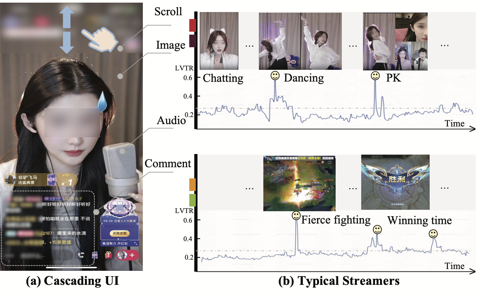
Figure 1: The live streaming platform and typical streamers. (a) Cascading UI of live streaming. (b) Highlight moments of two typical streamers.

Although plenty of methods [1, 2, 3, 4] have proposed to process frames or text in videos, the application and research in live streaming still suffer from lots of difficulties. First, unlike videos, live streaming makes predictions only based on information available up until that moment. Besides, multimodal information in these untrimmed videos is usually misaligned. For example, the reaction of hosts and audiences can experience a time lag, so the streamer’s speech and audiences’ comments may be ambiguous and not sequentially aligned with the visual frames, necessitating a module to mitigate the noise caused by misalignment. Moreover, there is no large-scale public dataset for live streaming highlight detection. AntPivot [5] propose a dataset called AntHighlgiht, but it only provides 3,656 samples with only textual feature. Hence, a large-scale live streaming dataset with multimodal information is crucial to assessing this topic.

In this paper, we propose a transformer-based network, which leverages multi-modality features for live streaming highlight prediction. First, we formulate the task as a prediction task based on historical look-back windows and the casual attention mask is proposed to avoid the information leakage from the future. Second, to alleviate the misalignment between visual and textual modality, we develop a novel Modality Temporal Alignment Module to address potential temporal discrepancies that may arise during live streaming events. Finally, we construct a large-scale live streaming dataset, named KLive, which provides segment-level content information like visual frames, comments and ASR results. Different from previous highlight datasets which use binary labels (highlight or non-highlight frames), KLive provides dense annotations and is more precise in reflecting the users’ general preferences on live streaming content. Based on KLive, we design a novel Border Aware Pairwise Loss with first-order difference constraints. We find that the constraints are essential when jointly optimizing pointwise and pairwise losses to avoid collisions and model collapse. We perform comprehensive experiments on both the large-scale real-world live streaming dataset KLive and a public PHD dataset [1] and achieve state-of-the-art performance. In summary, the main contributions made in this work are as follows:

• We propose a multimodal transformer framework for highlight detection in live streaming. For alleviating cross-modality misalignment, a modality Temporal Alignment Module is further presented to tackle this challenge.

• We provide a new dataset, called KLive, and design a Border Aware Pairwise Loss with first-order difference constraints to exploit the contrastive information of highlight frames and no-highlight frames.

• Extensive experiments are conducted on both KLive and public PHD dataset, and our model achieves state-of-the-art performance. We also present ablation and visualization results to demonstrate the effectiveness.

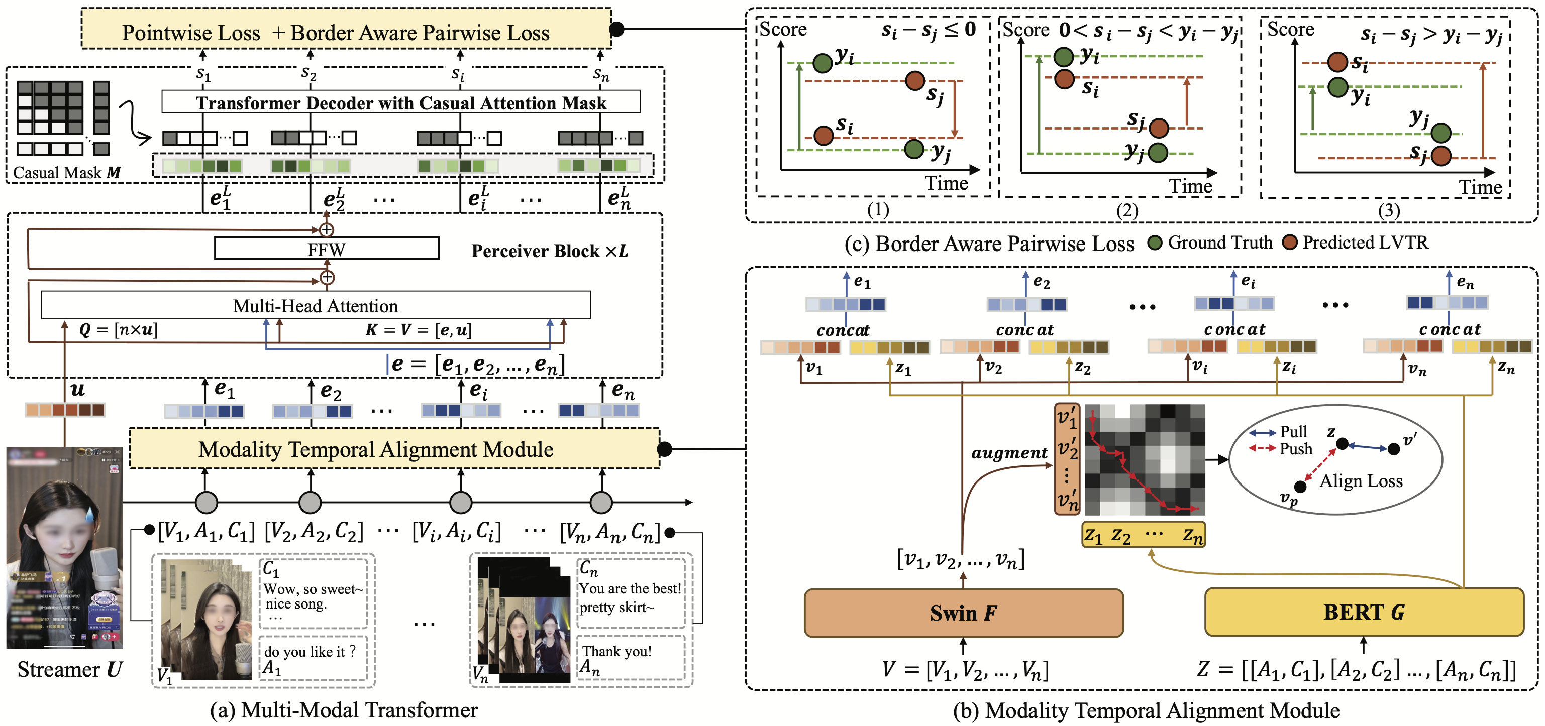
Figure 2: The framework of our method. Part (a) shows the architecture of Perceiver Block and Casual Attention Decoder which are discussed in Sect.III-B. Part (b) shows the proposed Modality Temporal Alignment Module which is discussed in Sect.III-C. Part (c) shows the motivation of Border-aware Pairwise Loss which is discussed in Sect.III-D.

II Related Work

II-A Video Highlight Detection

The task most closely related to streaming highlight prediction is Video Highlight Detection, as both aim to identify different content patterns in temporal sequences. Previous works such as dppLSTM [6] and Video2GIF [7] attempt to exploit temporal dependence from both past and future content. However, these works fail to adapt to live streaming scenarios without future frames. Recently, several works [1, 2, 8, 4, 3] try to further extract user-adaptive highlight predictions guided by annotated user history. For example, PHD-GIFs [1] is the first personalized video highlight detection technique that also creates a large-scale dataset called PHD. [4] design a DBC module to generate user-adaptive highlight classifier. [3] focus on leveraging the visual contents of both preferred clips and the target videos. We will compare with the above baselines to prove the effectiveness of our model.

II-B Live Streaming Highlight Detection

To the best of our knowledge, the concept of Live Streaming Highlight Detection (LSHD) is initially defined by [5]. The task seeks to retrieve corresponding frames for highlight topics and discussions. They propose a novel Pivot Transformer to capture temporal dependencies and integrate hierarchical semantic levels. They also construct a dataset called AntHighlight for streaming highlight detection. However, this work mainly considers the conversation interaction. And AntHighlight provides 3,656 records with speech modality information while our propose dataset provides multimodal information and more dense highlight labels.

III Methodology

III-A Problem Formulation and Model Overview

As shown in Figure 1 (a), the live streaming frame $\delta_{i}$ is shown to user with cascading UI. The streaming content will automatically play in this UI and users can choose to stop viewing current streaming room by scrolling to the last or next streaming room. Therefore, the view time becomes an important signal to reflect the live streaming content quality, which correlates with the occurrence of highlight moments. We define the impression whose watching time is greater than a threshold as long-viewing impressions. Note an impression is defined as an instance when live streaming frame $\delta_{i}$ was recommended to a user [9]. Then, the Long View Through Rate (LVTR) is calculated as follows:

$$LVTR=\frac{\mathrm{Number}\ \mathrm{of}\ \mathrm{Long}\ \mathrm{View}\ \mathrm{Impressions}}{\mathrm{Number}\ \mathrm{of}\ \mathrm{the}\ \mathrm{Total}\ \mathrm{Impressions}}$$ (1)

From the Figure 1 (b), we find that the high points of the LVTR curve usually correspond to the highlight moments. So we formulate the live streaming highlight prediction task by predicting the LVTR of frame $\delta_{i}$. We denote $M_{i}=\{V_{i},A_{i},C_{i}\}$ as the multi-modal tuple, where $V_{i},A_{i}$ and $C_{i}$ represent the visual, audio and comments of frame $\delta_{i}$. Note that we use Automatic Speech Recognition (ASR) to extract information from audio. For frames $\delta_{i}$ at timestamp $i$, the corresponding frames feature $v_{i}$ and concated ASR and comments text feature $z_{i}$ are extracted as follows:

$$v_{i}=F\left(V_{i}\right),z_{i}=G\left(\left[A_{i},C_{i}\right]\right)$$ (2)

where $F(\cdot)$ is a swin and $G(\cdot)$ is BERT. We concatenate $v_{i}$ and $z_{i}$ as the final input tokens $e_{i}$. Since the highlight pattern and audience taste change over time, the model should use the multi-modal information from the $n-1$ lookahead windows $e=[e_{i-n+1},e_{i-n+2},\cdots,e_{i-1}]$ of previous frames to predict the LVTR $y_{i}$ of frame $\delta_{i}$.

In this work, the multi-modal features will interact with ID embedding by the Perceiver Block and Casual Attention Decoder defined in Sect. III-B and be aligned by the Modality Temporal Alignment Module in Sect. III-C. Finally, the model will be optimized by the Pointwise and Pairwise loss defined in Sect. III-D.

III-B Perceiver Block and Casual Attention

Perceiver Block We hypothesize that different streamers have distinct talents and attract different audiences. For instance, as shown in Figure 1 (b), some audiences like dancing, while others may be attracted to the PK events between streamers. Therefore, we use separated ID embeddings $u$ for streamer $U$ to extract streamer-aware multimodal features (see Figure 2 (a)). Note $u$ will be repeated $n$ times to match the sequence length of the multimodal features $e$. First, we initialize learned latent query $Q$ with flattened $n\times u$. Next, we concatenate the flattened $e$ and $n\times u$ at the second dimension and take $K=V=[e,n\times u]$ as key and value. Then we perform standard scaled dot-product multi-head attention on the projected vectors with feed-forward network and residual connections. The Perceiver block is stacked for $L$ layers and the final output of Perceiver block is denoted by $e^{L}$.

Transformer Docoder We unflatten and squeeze the output of Perceiver block $e^{L}$ as the dimension of $\mathcal{R}^{b\times n\times d}$. Then we initialize the query, key and value of the decoder as $Q=K=V=e^{L}$ and we apply the scaled dot-product attention function with casual attention as follows:

$$\operatorname{Attention}(Q,K,V)=\operatorname{softmax}\left(\frac{QK^{\top}}{\sqrt{d_{h}}}+M\right)\cdot V$$ (3)

where $M$ is the casual attention mask and $d_{h}$ is the hidden dimension. As shown in Figure 2 (a), it is an $n\times n$ matrix filled with -inf and its upper triangular sub-matrices are filled with 0. By applying the casual attention mask $M$ the problem of future information leakage in the temporal dimension is avoided. The output from the final attention layer is then fed into a fully connected layer, followed by a sigmoid transformation to produce the scalar prediction of LVTR $s$.

III-C Modality Temporal Alignment Module (MTAM)

The motivation behind for alignment is to address potential temporal discrepancies that may arise during live streaming events. For example, the streamer may describe the plan before taking action, or explain detailed information after action. Additionally, the comments from the audiences may experience some time lag, which further exacerbates the misalignment issue. Therefore, it is essential to train text and visual encoders that can handle misalignment to alleviate that problem. Inspired by previous works [10], in this section we present our contrastive learning-based framework for visual and text sequence alignment.

In order to align $z$ and $v$ with optimal matching correspondence while considering the constraint of temporal order, we utilize the Dynamic Time Warping (DTW) algorithm by calculating the minimum cumulative matching cost between two sequences. Specially, we first compute a pairwise distance matrix $D\left(z,v\right)\coloneqq\left[\mathrm{sim}\left(z_{i},v_{j}\right)\right]_{ij}\in\mathcal{R}^{n\times n}$ with a distance measure $\mathrm{sim}(\cdot)$. In our work, we apply the cosine similarity as $\mathrm{sim}(\cdot)$. Then, we employ dynamic programming and sets a matrix $H\in\mathcal{R}^{n\times n}$ to record the minimum cumulative cost between $z_{i}$ and $v_{j}$:

$$H_{i,j}=D_{i,j}+\min\left\{H_{i-1,j-1},H_{i-1,j},H_{i,j-1}\right\}$$ (4)

where $1\leq i,j\leq n$. Then, the distance $d_{\left\{z,v\right\}}$ between sequences $z$ and $v$ is set to the last element of matrix $C$:

$$d_{\left\{z,v\right\}}=H_{n,n}$$ (5)

However, the standard DTW cannot solve the non-sequential alignments since it allows only three movement directions $\left\{\downarrow,\searrow,\rightarrow\right\}$. To tackle this problem, we propose a novel augmentation method to partially shuffle the original video sequence. Let $\omega$ denote all possible time index pair combinations retrieved from $v$, we formulate the target distribution as follows:

$$p^{video}=\mathrm{softmax}\left(\frac{D\left(z,v\right)_{ij}}{\gamma}\right),\left(i,j\right)\in\omega$$ (6)

where $\gamma$ is a temperature parameter. The proposed target distribution is more likely to generate a time index pair that has the most similarity between $z$ and $v$. Then, the index pair $(i,j)\sim P^{video}$ is sampled from the distribution $P^{video}$ defined in Equation 6 and we swap the corresponding values of $v$ to generate a new positive sample $v^{{}^{\prime}}$. In this way, the positive sample $v^{\prime}$ is more likely to have a more optimal temporal alignment order with $z$. Because compared to the original sequence $v$, there may exist no sequential alignment instances between original $v$ and $z$. We hypothesize that the positive pair $\left\{z,v^{{}^{\prime}}\right\}$ should be similar, while the negative pair $\left\{z,{v}_{p}\right\}$ should be dissimilar, where ${v}_{p}$ is directly shuffled from $v$. Consequently, we can formulate the training objective as minimizing the well-known InfoNCE loss:

$$\mathcal{L}_{align}=-\log\frac{\exp\left(d_{\left\{z,v^{{}^{\prime}}\right\}}/\tau\right)}{\exp\left(d_{\left\{z,v^{{}^{\prime}}\right\}}/\tau\right)+\sum_{v^{i}_{p}\in\omega}^{N}{\exp}\left(d_{\left\{z,v^{i}_{p}\right\}}/\tau\right)}$$ (7)

where $N$ is the number of negative samples directly shuffled from $v$. As shown in Figure 2 (b), by minimizing the align loss $\mathcal{L}_{align}$, the visual encoder $F(\cdot)$ and text encoder $G(\cdot)$ are encouraged to learn a good representation from aligned and misaligned pairs.

III-D Border Aware Pairwise Loss

The objective of pointwise loss is to maximize the log-likelihood between the predicted LVTR $s$ and the actual LVTR $y$, which can be achieved using the following pointwise model to optimize the standard LogLoss [11]:

$$L_{Point}=-\frac{1}{n}\sum_{i=1}^{n}\left[y_{i}\cdot\log\left(s_{i}\right)+(1-y_{i})\cdot\log\left(1-s_{i}\right)\right]$$ (8)

However, the pointwise loss defined in Equation 8 may fail to effectively exploit the contrastive information between the highlight and no-highlight frames. Therefore, we introduce the pairwise loss for further optimization. In this section, we present some intriguing discoveries on the traditional pairwise logistic ranking loss [12] and propose modifications to the loss function by integrating the border-aware first-order difference constraint.

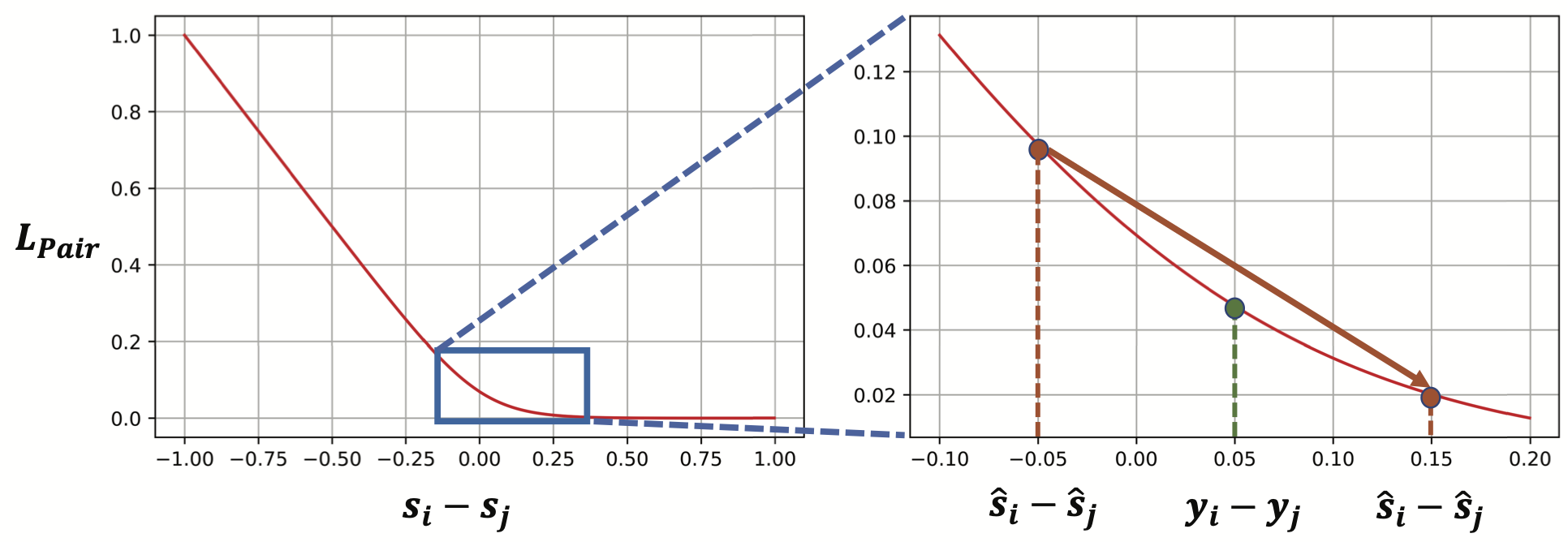
Figure 3: The change of pairwise loss function w.r.t. $s_{i}-s_{j}$ .

Consider the following pairwise loss function, which has no constraints:

$$L_{Pair}^{0}=\sum_{y_{i}>y_{j}}{\log\left(1+e^{-\sigma\left(s_{i}-s_{j}\right)}\right)}$$ (9)

where $y_{i}$ and $y_{j}$ are the ground truth LVTR at timestamps $i$ and $j$, $s_{i}$ and $s_{j}$ is the predicted LVTR from the model and $\sigma$ is a scale hyperparameter. Figure 3 illustrates the changing of the loss function $L_{Pair}$ with respect to $s_{i}-s_{j}$, which reveals that minimizing $L_{Pair}$ tends to cause $s_{i}-s_{j}$ to overtake the optimal value of $y_{i}-y_{j}$. This leads to over-optimization.

Based on the above findings, we propose a revised pairwise loss with a border-aware first-order difference constraint:

$$L_{Pair}^{1}=\sum_{y_{i}>y_{j}}{\log\left(1+e^{-\sigma\left(s_{i}-s_{j}\right)}\right)},\left(y_{i}-y_{j}\right)-\left(s_{i}-s_{j}\right)\geqslant 0$$ (10)

where $\left(y_{i}-y_{j}\right)-\left(s_{i}-s_{j}\right)\geqslant 0$ denotes the border, and solely those samples that reside within the border will calculate $L_{Pair}^{1}$. Any samples located outside the border will result in $L_{Pair}^{1}$ being set to 0.

Without losing generality, the original pairwise loss function $L_{Pair}^{0}$ presented in Equation 9 can be divided into three distinct parts:

• Part 1: As shown in Figure 2 (c1), when $s_{i}-s_{j}\leq 0$, the model’s assessment of the significance between timestamp $i$ and $j$ is entirely incorrect, given that timestamp $i$ is more "highlighting" than timestamp $j$.

• Part 2: As shown in Figure 2 (c2), when $0<s_{i}-s_{j}<y_{i}-y_{j}$, it implies that the model has distinguished that timestamp $i$ is more "highlighting" than timestamp $j$, but it still fails to accurately predict the difference in LVTR values between the two timestamps, and thus, it is still not optimal.

• Part 3: As shown in Figure 2 (c3), when $y_{i}-y_{j}<s_{i}-s_{j}$, it indicates that the model’s predicted LVTR value is too aggressive, resulting in over-optimization.

In order to verify the above scenarios, we design the following loss functions:

$$L_{Pair}^{2}=\sum_{y_{i}>y_{j}}{\log\left(1+e^{-\sigma\left(s_{i}-s_{j}\right)}\right)},s_{i}-s_{j}\leq 0$$ (11)

where $s_{i}-s_{j}\leq 0$ means that it only optimizes on Part 1.

$$L_{Pair}^{3}=\sum_{y_{i}>y_{j}}{\log\left(1+e^{-\sigma\left(s_{i}-s_{j}\right)}\right)},y_{i}-y_{j}>s_{i}-s_{j}>0$$ (12)

where $y_{i}-y_{j}>s_{i}-s_{j}>0$ means that it only optimizes on Part 2. The ablation study among $L_{Pair}^{0}$, $L_{Pair}^{1}$, $L_{Pair}^{2}$ and $L_{Pair}^{3}$ is discussed in Section IV. In this work, we apply the $L_{Pair}^{1}$ for optimization.

By combining pointwise loss in section III-B, align loss in section III-C and pairwise loss, our final loss used to learn the model parameters is defined as:

$$\mathcal{L}=\lambda_{1}\mathcal{L}_{Point}+\lambda_{2}\mathcal{L}_{align}+\lambda_{3}\mathcal{L}_{Pair}^{1}$$ (13)

where $\lambda_{1}$, $\lambda_{2}$ and $\lambda_{3}$ are the tradeoff parameters.

TABLE I: Performances of different methods on KLive and PHD dataset

Methods		KLive Tau $\boldsymbol{\tau\uparrow}$				PHD mAP $\boldsymbol{\uparrow}$
		$\Delta=0$	$\Delta=0.2$	$\Delta=0.4$	$\Delta=0.6$
VHD Methods
Adaptive-H-FCSN [2]	[ECCV’20]	0.5782	0.5707	0.5511	0.5322	15.65
PR-Net [8]	[ICCV’21]	0.5848	0.5818	0.5461	0.5403	18.66
PAC-Net [4]	[ECCV’22]	0.5823	0.5845	0.5537	0.5409	17.51
ShowMe [3]	[MM’22]	0.5798	0.5705	0.5348	0.5407	16.40
LSHD Methods
AntPivot [5]	[arXiv’22]	0.5818	0.5809	0.5483	0.5421	-
KuaiHL	[Ours]	0.5961	0.5871	0.5686	0.5563	21.89

IV Experiments

In this section, we perform experiments with KLive and PHD dataset and present the experimental results and some analysis of them. Please refer to the supplementary material for more information of dataset and implementation details. Our code is available at https://github.com/ICME24/KLive.

IV-A Dataset

To comprehensively evaluate the model’s performance, we show results on both KLive and public PHD dataset [1].

KLive Dataset We construct a large-scale dataset that contains 17,897 high-quality live rooms (19,334 hours) from a well-known live streaming platform. Each live room is divided into multiple consecutive 30s live segments, with three pictures evenly sampled for each segment, the streamer’s ASR and audiences’ comments. We employ consecutive 20 segments as a sample and obtain 1,436,979 and 286,510 samples for training and test datasets. Because the objective is to predict the LVTR of future frames, we left shift the ground truth for all live segments as the final label.

PHD Dataset To verify the generality of our method, we evaluate on the publicly available video highlight detection dataset [1] (PHD). The training set comprises of 81,056 videos, while the testing set has 7,595 videos. Please refer to supplementary material for more details.

IV-B Evaluation Metrics

For the experiments on KLive dataset, we employ rank correlation coefficients Kendall’s tau $\tau$ [13] to measure the correlation between our predicted LVTR $s$ and the ground truth LVTR $y$. We also report the various levels of Kendall’s tau agreement for the live frames whose ground truth LVTR is greater than the threshold $\Delta$. On PHD dataset, we utilize the widely adopted mean Average Precision (mAP) as a metric to evaluate the performance of our method, which is also applied in previous works [3, 4, 8, 2] in video highlight detection. We report the mAP on the test set and follow the way in [4] to calculate the mAP.

IV-C Overall Performance Comparison

Table I summarizes the LVTR prediction performances achieved by various methods on KLive and PHD dataset. On the KLive dataset, KuaiHL exhibits superior performance compared to all VHD and LSHD methods across various threshold levels, surpassing the LSHD method AntPivot which only models the text modality by +1.43% in tau. Similarly, on PHD dataset, KuaiHL outperforms the strongest baseline PR-Net [8] by +3.23%.

IV-D Border Aware Pairwise Loss and MTAM

We investigate the impact of different loss functions on KLive dataset, which include $L_{Point}$, $L_{Pair}^{0}$, $L_{Pair}^{1}$, $L_{Pair}^{2}$, $L_{Pair}^{3}$, and $L_{align}$ (Note that alignment loss without the augmentation method defined in Equation 6 is represented as $L_{align}^{{}^{\prime}}$).

TABLE II: Ablation study of KuaiHL with different loss functions on KLive dataset.

Methods	$\boldsymbol{L_{Point}}$	$\boldsymbol{L_{Pair}^{0}}$	$\boldsymbol{L_{Pair}^{1}}$	$\boldsymbol{L_{Pair}^{2}}$	$\boldsymbol{L_{Pair}^{3}}$	$\boldsymbol{L_{align}^{{}^{\prime}}}$	$\boldsymbol{L_{align}}$	Tau $\boldsymbol{\tau}$
(a)	✓	-	-	-	-	-	-	0.5761
(b)	✓	✓	-	-	-	-	-	0.5857 $\uparrow$ 0.96%
(c)	✓	-	✓	-	-	-	-	0.5872 $\uparrow$ 1.11%
(d)	✓	-	-	✓	-	-	-	0.5256 $\downarrow$ 5.05%
(e)	✓	-	-	-	✓	-	-	0.5824 $\uparrow$ 0.66%
(f)	✓	-	✓	-	-	✓	-	0.5919 $\uparrow$ 1.58%
(g)	✓	-	✓	-	-	-	✓	0.5961 $\uparrow$ 2.00%

When Method (b) optimizes $L_{Point}$ with unconstrained pairwise loss $L_{Pair}^{0}$, it shows a performance improvement of +0.96%. However, we have noticed that during training, the pointwise loss of Method (b) tends to collapse due to the over-optimization of pairwise loss in Part 3, which is shown in Figure 4. So we investigate the performance of different versions of constrained pairwise loss with Method (c), (d) and (e). We find that Method (c) which is jointly optimized on Part 1 and Part 2 with $L_{Pair}^{1}$ shows a significant improvement of +1.11% and both losses remain normal in Figure 4. Method (e) only shows a performance improvement of +0.66%, while Method (d) with $L_{Pair}^{2}$ shows a significant performance degradation of -5.05%. We hypothesize that the gradient changes are too drastic when optimizing only Part 1, which is detrimental to modeling the contrastive information of highlight frames and non-highlight frames. Therefore, we apply $L_{Pair}^{1}$ for final optimization.

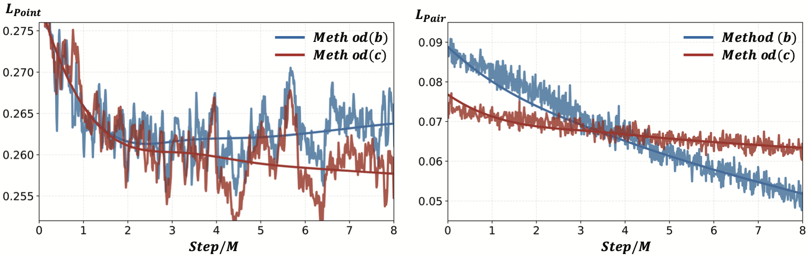
Figure 4: The change of $L_{Point}$ and $L_{Pair}$ during training.

We also investigate the influence of MTAM alignment and our proposed augmentation method defined in Equation 6. When Method (f) incorporates $L_{align}^{{}^{\prime}}$ for optimization, the naive DTW alignment loss achieves improvement with +1.58%. By applying our proposed novel augmentation method to generate the positive sample, Method (g) gains further improvement by +0.42%.

Figure 5 (a) shows some visualizations of DTW alignment results for the KLive dataset, which reveal that misalignment cases do exist in streaming scenarios. Figure 5 (b) presents a frame sequence and corresponding activities for one of the streaming scenarios. Here, the streamer shows her singing talent, where $a\rightarrow b$ indicates her interaction with the audience, resulting in aligned visual frames and text. However, during the transition from $b\rightarrow c$, the streamer starts singing, causing the text to become the lyrics of the song, resulting in a misalignment with the visual frames. As a result, the path becomes vertical. During $c\rightarrow d$, the streamer engages in a PK competition with another streamer. However, during $d\rightarrow e$, the frames from the other streamer get stuck due to network issues. Consequently, the visual frames become misaligned with text, causing the path to become horizontal. This case indicates that the involvement of $L_{align}$ does help our model in training better visual and text encoders that reduce the possible misalignment between the two.

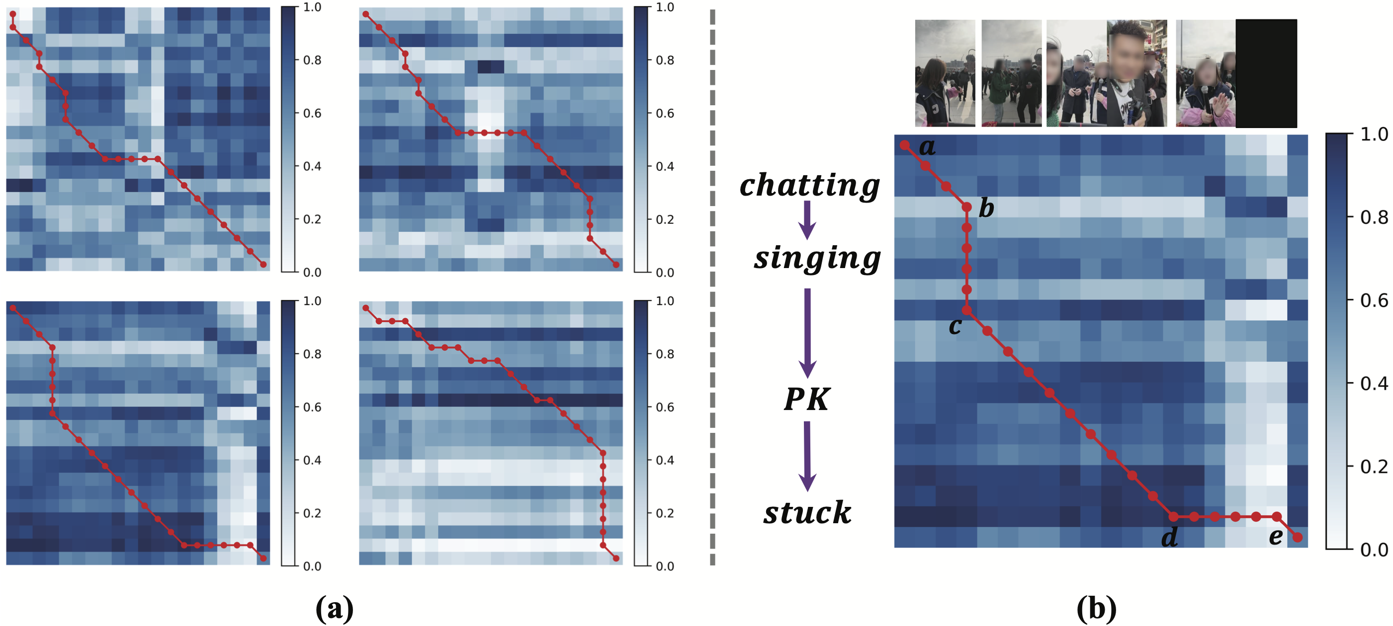
Figure 5: Visualization of Dynamic Time Warping (DTW) alignment results for the KLive dataset.

IV-E Modality Impact

As shown in Table III, on KLive we find visual modality has the most important impact, causing a performance degradation of -4.72% when removed. The text modality is the second most significant factor, while the ID embedding has the smallest but still significant effect on the model’s performance. On PHD dataset, the visual feature is more important than the captions modality.

TABLE III: Ablation study on different modality impact.

Model	$v$	$a$	$x$	$u$	$c$	Tau $\tau$	mAP(%)
KLive dataset
KuaiHL	✓	✓	✓	✓	-	0.5961	-
KuaiHL w/o item	✓	✓	✓	-	-	0.5910 $\downarrow$ 0.51%	-
KuaiHL w/o text	✓	-	-	✓	-	0.5760 $\downarrow$ 2.01%	-
KuaiHL w/o visual	-	✓	✓	✓	-	0.5489 $\downarrow$ 4.72%	-
PHD dataset
KuaiHL	✓	-	-	-	✓	-	21.89
KuaiHL w/o visual	-	-	-	-	✓	-	19.55 $\downarrow$ 2.34%
KuaiHL w/o caption	✓	-	-	-	-	-	20.06 $\downarrow$ 1.11%

V Conclusion

In this paper, we introduce a model called KuaiHL which utilizes a multimodal transformer to achieve frame-level LVTR prediction. Specifically, we propose a streamer-personalized Perceiver Block that fuses ID embedding, visual, audio, and comment embedding. The decoder network outputs the final LVTR prediction for each frame. To address the possible misalignment between video frames and texts, we carefully design a Modality Temporal Alignment Module for optimization. Additionally, the border-aware constrained pairwise loss demonstrates better performance when combined with the pointwise loss. We conduct comprehensive experiments on both the KLive dataset and the public PHD dataset, which demonstrate the effectiveness of our methods in both streaming LVTR prediction and video highlight detection tasks. Moreover, the proposed method has been deployed online on the company’s short video platform and serves over three million daily users.

References

- [1] Ana Garcia del Molino and Michael Gygli, “Phd-gifs: personalized highlight detection for automatic gif creation,” in Proceedings of the 26th ACM international conference on Multimedia, 2018, pp. 600–608.
- [2] Mrigank Rochan, Mahesh Kumar Krishna Reddy, Linwei Ye, and Yang Wang, “Adaptive video highlight detection by learning from user history,” in Computer Vision–ECCV 2020: 16th European Conference, Glasgow, UK, August 23–28, 2020, Proceedings, 2020, pp. 261–278.
- [3] Uttaran Bhattacharya, Gang Wu, Stefano Petrangeli, Viswanathan Swaminathan, and Dinesh Manocha, “Show me what i like: Detecting user-specific video highlights using content-based multi-head attention,” in Proceedings of the 30th ACM International Conference on Multimedia, 2022, pp. 591–600.
- [4] Hang Wang, Penghao Zhou, Chong Zhou, Zhao Zhang, and Xing Sun, “Pac-net: Highlight your video via history preference modeling,” in Computer Vision–ECCV 2022: 17th European Conference, Tel Aviv, Israel, October 23–27, 2022, Proceedings, Part XXXIV. Springer, 2022, pp. 614–631.
- [5] Yang Zhao, Xuan Lin, Wenqiang Xu, Maozong Zheng, Zhengyong Liu, and Zhou Zhao, “Antpivot: Livestream highlight detection via hierarchical attention mechanism,” arXiv preprint arXiv:2206.04888, 2022.
- [6] Ke Zhang, Wei-Lun Chao, Fei Sha, and Kristen Grauman, “Video summarization with long short-term memory,” in Computer Vision–ECCV 2016: 14th European Conference, Amsterdam, The Netherlands, October 11–14, 2016, Proceedings, Part VII 14. Springer, 2016, pp. 766–782.
- [7] Litong Feng, Ziyin Li, Zhanghui Kuang, and Wei Zhang, “Extractive video summarizer with memory augmented neural networks,” in Proceedings of the 26th ACM international conference on Multimedia, 2018, pp. 976–983.
- [8] Runnan Chen, Penghao Zhou, Wenzhe Wang, Nenglun Chen, Pai Peng, Xing Sun, and Wenping Wang, “Pr-net: Preference reasoning for personalized video highlight detection,” in Proceedings of the IEEE/CVF International Conference on Computer Vision, 2021, pp. 7980–7989.
- [9] Ashutosh Nayak, Mayur Garg, and Rajasekhara Reddy Duvvuru Muni, “News popularity beyond the click-through-rate for personalized recommendations,” in Proceedings of the 46th International ACM SIGIR Conference on Research and Development in Information Retrieval, 2023, pp. 1396–1405.
- [10] Dohwan Ko, Joonmyung Choi, Juyeon Ko, Shinyeong Noh, Kyoung-Woon On, Eun-Sol Kim, and Hyunwoo J Kim, “Video-text representation learning via differentiable weak temporal alignment,” in Proceedings of the IEEE/CVF Conference on Computer Vision and Pattern Recognition, 2022, pp. 5016–5025.
- [11] Tie-Yan Liu et al., “Learning to rank for information retrieval,” Foundations and Trends® in Information Retrieval, vol. 3, no. 3, pp. 225–331, 2009.
- [12] Chris Burges, Tal Shaked, Erin Renshaw, Ari Lazier, Matt Deeds, Nicole Hamilton, and Greg Hullender, “Learning to rank using gradient descent,” in Proceedings of the 22nd international conference on Machine learning, 2005, pp. 89–96.
- [13] Yassir Saquil, Da Chen, Yuan He, Chuan Li, and Yong-Liang Yang, “Multiple pairwise ranking networks for personalized video summarization,” in Proceedings of the IEEE/CVF International Conference on Computer Vision, 2021, pp. 1718–1727.