From Top-Right to User-Right:
Perceptual Prioritization of Point-Feature Label Positions

Abstract

In cartography, Geographic Information Systems (GIS), and the entire field of visualization, the position of a label relative to its point feature is pivotal for ensuring visualization readability and improving the user experience. The label placement is governed by the Position Priority Order (PPO), a systematic raking of potential label positions around a point feature according to predetermined priorities. Traditional PPOs have relied heavily on typographic and cartographic conventions established decades ago, which may no longer align with the expectations of today’s users. Our extensive user study introduces the Perceptual Position Priority Order (PerceptPPO), a user-validated PPO that significantly departed from traditional conventions. A key finding of our research is the identification of an exact order of label positions, with labels placed at the top of point features being significantly preferred by users, contrary to the conventional top-right position. Furthermore, we performed a supplemental user study to find users’ preferred label density – an area scarcely explored in prior research – of a generic map. According to the results, users prefer, on average, 17% of the generic map to be covered by labels. Finally, we performed a comparative user study assessing the perceived quality of PerceptPPO compared to existing PPOs. The outcome confirmed PerceptPPO’s superior perception among users, advocating its adoption not only in future cartographic and GIS applications but also across various types of visualizations. The effectiveness of PerceptPPO in aligning label placement with user preferences is supported by nearly 800 participants from 48 countries, who collectively contributed to over 45,500 pairwise comparisons across three studies. Our research not only proposes a novel PPO to the research community but also offers practical guidance for designers and application developers aiming to optimize user engagement and comprehension, paving the way for more intuitive and accessible visual solutions.

K.6.1Management of Computing and Information SystemsProject and People ManagementLife Cycle; K.7.mThe Computing ProfessionMiscellaneousEthics *[inlinelist,1]label=(0),

Introduction

Automatic label placement holds a crucial role across various domains such as cartography, data visualization, and geographic information systems (GIS), facilitating clear communication and enhancing the user’s ability to interpret the underlying data. Short textual annotations, or labels, play an important part in enhancing the comprehension of visualized data, not only in maps but across various visual representations. Labels convey essential information about distinct data points, ranging from cities and landmarks within cartographic contexts to pivotal elements in diagrams, charts, and geographic information systems (GIS). Recognized by the ACM Computational Geometry Impact Task Force [2] as an area of significant research interest, the challenge of optimally positioning textual annotations remains a vibrant field of study, especially concerning point-feature label placement (PFLP).

Point-feature label placement primarily deals with the maximization problem – aiming to position labels for the maximum number of point features, also called anchors, possible within a given set. This task is often constrained by the fixed-position model, which restricts label placements to a limited number of predefined positions around a point feature. This limitation necessitates using a systematic order of preference for these positions, which we term as Position Priority Order (PPO). The PPO ranks potential label positions according to predetermined priorities, guiding the selection process.

However, a closer review of existing literature reveals a disconcerting lack of consensus in PPOs as described in detail in section 1. Various authors have ascribed different priorities to the same label positions, often without a clear or unified rationale. Priorities have historically been based on typographic and cartographic conventions, with varying degrees of justification and consistency across the literature, leading to a fragmented understanding of optimal label placement practices. The identified inconsistency highlights a gap in the field and underlines the necessity for an empirically grounded methodology that reflects user perceptions and preferences.

Our research introduces Perceptual Position Priority Order (PerceptPPO), a user-centered methodology that seeks to redefine the prioritization of point-feature label positions based on users’ perceptual and cognitive preferences rather than traditional conventions. Through this effort, we aim to establish a new standard in automatic label placement that prioritizes user experience, paving the way for more intuitive and accessible map designs and setting a precedent for future research in the domain. Our main contributions are summarized as follows:

1. We propose a comprehensive review of existing literature on Position Priority Orders (PPOs), analyzing existing PPOs and highlighting the missing consensus based on user preferences.

2. We introduce Perceptual Position Priority Order (PerceptPPO), a novel, user-centered prioritization of point-feature label positions that prioritizes user perceptions and preferences over traditional conventions supported by a global user study involving nearly 800 participants from 48 countries.

3. We uncover the optimal label density for maps, an aspect seldom explored in prior research, revealing a user preference for 17% label coverage on generic maps.

4. We provide analysis demonstrating the superior user preference of PerceptPPO over existing PPOs, reinforcing its potential for improving map design, user experience in cartographic applications, and other types of visualizations.

1 Related Work

In the domain of point-feature label placement, the primary challenge involves the selection of the most appropriate position for each label from among $n$ potential candidates surrounding a point feature, with the objective of maximizing the number of labels that can be placed. When multiple suitable position candidates are available for a point feature, the selection is determined based on the Position Priority Order (PPO) of the label candidates, an assigned value within the range $[1,n]$, where a lower value means a higher priority.

Within the cartographic community and the domain of automated label placement, a variety of position models have been utilized, differing in the number of label candidates considered for each point feature. The 8-position model is the most prevalent, evaluating eight potential label placements per point feature, followed in popularity by the 6-position, 4-position, and 10-position models, respectively. Figure 1 illustrates the label candidate positions for these models. Models with alternative configurations, such as the 5-position model, are used rarely.

Alongside the position models, authors frequently delineate the priorities assigned to label candidates. However, our review of the existing literature reveals inconsistencies and, at times, contradictions in these priorities. This section presents our analysis of point-feature labeling practices. Tab. 1 shows the analyzed works detailing their chosen position models and the associated priorities. We have categorized the literature into four groups based on the similarity of their priority schemes. A fifth category encompasses works with distinct priority practices that do not align with those of any other group.

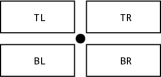
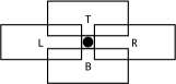
Figure 1: Common label positions for a point feature as presented in prior literature: 1 4-position model, 1 additional positions of 8-position model, and 1 additional positions of 10-position model.

Author Year Citations Type Position Priority Order 1 2 3 4 5 6 7 8 9 10 YoeliA [23] 1972 231 A TR TL BR BL T B Robinson et al. [14] 1995 (6th) 3096 (4th) B TR TL BR BL T B T_SR B_SR T_SL B_SL Brewer [1] 2015 441 B TR TL BR BL T B YoeliB [23] 1972 231 A TR TL BR BL R L T B Dent [5] 2009 (6th) 1304 (5th) B TR TL BR BL R L T_SL B_SR Dobias (QGIS) 2009 – SW TR TL BR BL R L T_SR B_SR Krygier et al. [12] 2016 (3rd) 361 B TR TL BR BL R L T_SL B_SR Christensen and Marks [3] 1995 520 A TR TL BL BR R T L B Yamamoto [22] 2005 40 A TR TL BL BR Ebinger and Goulette [6] 1989 – A TR BR TL BL Wood [21] 2000 28 A TR BR TL BL T_SR B_SL Slocum et al. [16] 2022 (4th) 962 B TR BR TL BL T B R L Imhof [9] 1975 (^∗1962) 439 (^∗88) A TR R T B L Zoraster [24] 1986 108 A TR T R TL BR L B BL Jones [10] 1989 79 A TR R BR TL L BL Zoraster [25] 1990 129 A TR T TL R L BR B BL Zoraster [26] 1997 103 A T TR TL R L BR B BL PerceptPPO 2024 – A T B R TR BR L TL BL

Table 1: This overview outlines the PPO recommendations of various authors grouped by similarity. The top-right (TR) positioning emerges as a dominant preference, with authors consistently favoring it. While TR remains widely accepted across the board, there is noticeable diversity in selecting other positions. The citation counts are derived from Google Scholar. ^∗The seminal work, Die Anordnung der Namen in der Karte, was first introduced in German in 1962. Yoeli [23] and Zoraster [26] define more than 8 positions that are not included in our comparison as they are rarely used. Abbreviations: A – article, B – book, SW – software.

The initial guidelines for selecting appropriate label candidates, among other labeling rules, were formulated by Imhof in 1962, published in German, and later translated into English [9]. Imhof introduced a 5-position model tailored for left-to-right languages, leveraging his cartographic expertise to recommend the top-right position as the most favorable for label placement. His preference was rooted in typographic principles, e.g., the top position (T) was favored over the bottom (B). This rationale was based on the observation that in the Latin alphabet, ascenders are more common than descenders, suggesting that labels placed at the top are likely to appear visually closer to their corresponding point features. This consideration is particularly relevant for city names, which typically begin with a capital letter.

Yoeli [23] introduced the first algorithms for the automated positioning of point-feature labels. He proposes two n-position models later adopted for point-feature label placement by other authors. The first position model, denoted in Tab. 1 as YoeliA, is a 10-position model where the label candidates are organized around the point feature as in Figure 1. Notably, Yoeli proposed a grid system for typesetting the labels where the size of the grid cell is based on the size of the letters. Therefore, Yoeli distinguishes between labels with an odd and even number of letters. Since the latter cannot be centered above or below the point feature, Yoeli introduces additional top and bottom position modifiers that shift the label slightly left (SL) or slightly right (SR). In Tab. 1, we report only the first six positions, as nowadays, even labels with an even number of letters can be easily centered above or below the point feature. Similarly, Brewer [1] omits the four additional positions with shifted labels in his 6-position model. For Robinson et al. [14], we report all positions in his 10-position model with priorities identical to Yoeli’s, as he is not providing any information as to why the positions with shifted labels are included in his model.

The second position model, denoted in Tab. 1 as YoeliB, is an 8-position model that Yoeli originally crafted for labeling small-area features. Nonetheless, other authors [5, 12] adopted or adapted Yoeli’s 8-position model for point-feature label placement. Similarly, as in the previous 10-position model, Yoeli [23] uses additional top and bottom positions slightly shifted to the left for labels with an even number of letters. However, we again ignore additional adjustments for even-lettered labels, as they can be precisely centered directly above or below the point feature nowadays, regardless of letter count.

Christensen and Marks [3] introduced two algorithms for PFLP, employing gradient descent and simulated annealing techniques. The formulation of the proposed objective function draws upon Yoeli’s foundational work Yoeli [23]. Notably, they adopt an 8-position model similar to Yoeli’s, but with swapped priorities of bottom-left (BL) and bottom-right (BR) positions and the top (T) and left (L) positions, which they describe as a standard PPO.

Ebinger and Goulette [6] proposed a 4-position model, see Figure 1, which diverges in priority schemes from one proposed by Imhof [8] and Yoeli [23]. While Yoeli prioritizes top positions over bottom positions, Ebinger and Goulette prioritize positions on the right side over the left. Wood [21] proposed a 6-position model with the top position being shifted slightly right ($\mathrm{T_{SR}}$) and the bottom slightly left ($\mathrm{B_{SL}}$). The author remarks that the shifted positions should only be used in extreme cases. Moreover, he argues that the shifted positions help associate the label with the feature; unfortunately this claim is not supported by any justification. Similarly, Slocum et al. [16] proposed an 8-position model extending Wood’s first for positions to include top (T), bottom (B), right (R), and left (L) positions, enhancing label placement flexibility.

The prior literature exhibits even more significant variety in priority schemes for label placement. Zoraster [24, 25, 26], in his series of works, introduced three distinct 8-position models for oil well labeling, each with unique priorities. A notable trend across Zoraster’s models is the elevated priority given to the top position, starkly contrasting with other authors’ approaches. Additionally, Jones [10]) proposed 8-position models that resemble the 4-position model by Ebinger and Goulette [6], with a nuanced approach to prioritization: the right (R) position is placed between the top-right (TR) and bottom-right (BR) positions, while the left (L) position’s priority is set between the top-left (TL) and bottom-left (BL) positions.

Upon examining Tab. 1, it becomes clear that with the exception of Zoraster [26], the top-right (TR) position emerges as the highest priority across multiple bodies of work. The designation of priorities to other positions shows even more significant variability, highlighting a lack of consensus. Moreover, all reported priorities are based on the experience of the authors, and none of them were empirically verified by users. To our knowledge, the sole exception is a study by Scheuerman et al. [15], which attempts to evaluate position priorities with user input but limits its scope to just three positions (TL, L, BL). The study establishes the position preference order of $L>TL>BL$, indicating L is favored over TL and BL, and TL is preferred over BL.

The disparities and notable gap in evaluations set the stage for our investigation. We ask the question whether specific Position Priority Orders (PPOs) influence the perceived label placement quality and we aim to establish a set of priorities validated by user-centered research. This will pave the way for more intuitive and accessible mapping solutions firmly grounded in empirical evidence.

2 Perceptual Position Priority Order (PerceptPPO)

Due to non-existing consensus on the ranking of label positions within cartography and GIS, we aim to create PPO rooted in user perception. Typographic and cartographic conventions used in previous works are valuable, but originate from several decades-old practices that may not align with modern user needs. Herein, we detail the empirical user study that underpins PerceptPPO and lay the groundwork for a comparative analysis that underscores its efficacy.

2.1 Data

We randomly selected 30 locations worldwide. We excluded any locations on the sea or ocean and those with latitudes greater than -60 degrees to exclude Antarctica due to its sparse population. Each location served as the center of an area, defined by the location and a zoom level ranging from 5 (approximately the size of Europe) to 10 (roughly the size of Luxembourg), rendered as a vector SVG image at a size of $1305\times 1025$ pixels. Settlements with more than 500 habitants, obtained from GeoNames, specifically Cities 500, within these areas were used as anchors and were sorted by population size. Then we filtered only anchors such that all the 8-positions around are available in any configurations of labels without any conflict (we examined the occurrence of conflict for all anchors over bounding boxes containing all eight positions of labels). If an area contained fewer than 20 anchors, we discarded it in favor of another area. Finally, we acquired 30 areas indexed from 0 to 29 at zoom levels 5 to 8, with 20 to 54 anchors.

Subsequently, we rendered each area eight times, placing all labels in one of the eight corresponding positions relative to the anchor: top-right (TR), top (T), top-left (TL), left (L), bottom-left (BL), bottom (B), bottom-right (BR), and right (R). This process yielded $30\times 8=240$ blind maps featured with a white background, red anchors, and corresponding labels. See example in Figure 2 and suppl. material for all renders.

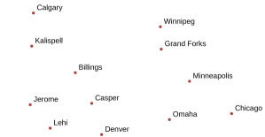
(a) TR

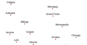
(b) T

Figure 2: Example of map area rendered consistently using TR and T position across all point features.

2.2 Procedure

We employed the Two-Alternative Forced Choice (2AFC) approach to determine the position priority order based on the actual perception of users, which we call Perceptual Position Priority Order (PerceptPPO). Considering the eight label positions under examination, we have ${{8}\choose{2}}=28$ pairwise comparisons on an area. Consequently, the entire experiment consists of $30\times 28=840$ pairwise comparisons to cover all of them once. In order to alleviate potential fatigue among the participants during the study, we allocated only three areas to each participant, resulting in a batch of $3\times 28=84$ pairwise comparisons. Therefore, 10 participants were required to cover all pairwise comparisons once.

We engaged Mechanical Turk workers and university students to conduct the experiment. Initially, the participants were introduced to the experiment and asked about their country of residence, age, gender, and education. Each participant was allowed to take only one batch of 84 pairwise comparisons to mitigate the carry-over effect. During the experiment, the pairs of area and label position were distributed randomly but uniformly between the left and right sides of the shown comparison pair. Participants were shown two maps sequentially, each depicting the same area but with different positions of labels relative to the anchors. Notably, the position of a label was kept consistent for all points within a single map, see Figure 2. Participants were asked to select the map they found aesthetically more pleasing from each presented pair. At the end of the experiment, the participants were allowed to leave an additional note about anything regarding the experiment.

2.3 Statistical Analysis

To derive insights from the pairwise comparison data of $n$ objects, we transform the data into the $n\times n$ preference matrix $P$ for each participant individually. Each element $p_{ij}$ in the matrix indicates the number of times that method $i$ was selected over method $j$ by a participant. The conversion allows for a preference analysis, facilitating the identification of PPO patterns across participants in the study.

2.3.1 Coefficient of Consistency $\zeta$

Assessing whether the particular participant can form a reliable judgment of the quality under examination is crucial when using paired comparison. Kendall and Babington [11] proposed coeficient of consistency $\zeta$ to measure the consistency based on the transitivity of participant’s choices. For example, when evaluating three objects: A, B, and C, a participant might choose that $A>B$ ($A$ is preferred to $B$), $B>C$ and $C>A$. In this case, the triad is called circular and the pair comparison inconsistent. The $\zeta=1$ if there are no circular triads / no inconsistencies. On the other hand, when the number of circular triads/inconsistencies increases, the $\zeta$ decreases towards zero. Inconsistency can arise due to incompetence, participant’s attention changes during the experiment, or the examined objects being too alike. The definition of $\zeta$ can be simplified as $\zeta=1-\frac{T}{T_{max}}$, where T is the observed number of circular triads, $T_{max}$ is the maximum number of circular triads. For more details, see Kendall and Babington [11] and David [4]. We employ the implementation of the EBA package proposed by Wickelmaier and Schmid [20], which also provides the expected number of circular triads $E(T)$ when choices are made at random. In particular, we identify participants as potentially inconsistent if $T<E(T)$ is observed in at least two of the three areas assigned for their evaluation.

2.3.2 Coefficient of Agreement $u$

While the coefficient of consistency provides a measure of consistency within participants, the coefficient of agreement $u$ introduced by Kendall and Babington [11] measures the variety of choices among $m$ participants. Complete agreement $u=1$ is achieved when all participants make identical choices for all pairs. In other words, the half $p_{ij}$ of the overall preference matrix $\mathbf{P}=\sum_{k\in(0,m)}P_{k}$ is equal to the number of participants $m$, while the other half is a zero. On the other hand, the minimum number of agreements occurs when $p_{ij}=\frac{m}{2}$ if $m$ is even or when $p_{ij}=\tfrac{m\pm 1}{2}$ otherwise. Correspondingly, minimum coefficient of agreement $u_{\mathrm{min}}=\tfrac{-1}{m-1}$ or $u_{\mathrm{min}}=\tfrac{-1}{m}$. For cases in between the $u$ range, Kendall and Babington [11] defines $u$ as

$$u=\frac{2\sum_{i\neq j}{p_{ij}\choose{2}}}{{{m}\choose{2}}{{n}\choose{2}}}-1.$$ (1)

The statistical significance of $u$ with the null hypothesis that all participants choose the preferences randomly (or there is no agreement among participants) can be approximated by $\chi^{2}$ variate as described in David [4]. Again, we employ the implementation of the EBA package proposed by Wickelmaier and Schmid [20].

2.3.3 Pairwise Comparison Model

To transform the preference matrices to quality scores, we employ Thurstone’s statistical judgment model proposed by Thurstone [17], as recommended by Tsukida and Gupta[18] and Pérez-Ortiz and Mantiuk [13]. The model assumes that the quality score of object A is a Normal random variable $A\sim N(q_{A},\sigma_{A})$ where $q_{A}$ is assumed to be the true quality score. Similarly, for object $B\sim N(q_{B},\sigma_{B})$. Normal distribution captures the fact that different participants have various preferences regarding the quality of examined objects (inter-participant variance). Moreover, participants’ preferences are also likely to change when they repeat the same experiment (intra-participant variance). We apply Thurstone’s Case V model, which assumes that a Normal distribution can explain inter- and intra-participant variance. At the same time, the $\sigma$ describes the uncertainty and is the same for all examined objects (in our example $\sigma_{A}=\sigma_{B}$) while correlation among objects is zero ($\rho_{AB}=0$). The difference between the two Normal distributions is again Normal distribution $A-B\sim N(q_{AB},\sigma_{AB})$. Without loss of generality, we can assume that variance $\sigma_{A}^{2}=\sigma_{B}^{2}=\tfrac{1}{2}$ so that $\sigma_{AB}^{2}=\sigma_{A}^{2}+\sigma_{B}^{2}-2\rho_{AB}\sigma_{A}\sigma_{B}=1$ which corresponds to standard Normal distribution. The quality difference estimation of two objects A and B $\hat{q}_{AB}$ is then defined as

$$\hat{q}_{AB}=\Phi^{-1}\left(\frac{P_{A,B}}{P_{A,B}+P_{B,A}}\right),$$ (2)

where $\Phi^{-1}(x)$ is the inverse CDF of standard Normal distribution that can be interpreted as z-score as it represents the distance of $x$ from the mean in units of the standard deviation.

To determine quality scores of $m$ objects, Tsukida and Gupta[18] recommend using the maximum likelihood estimate (MLE). To this end, we employ the MLE implementation of Pérez-Ortiz and Mantiuk [13], which also includes confidence interval estimation based on random sampling with replacement and methodology to perform a two-tailed test of the null hypothesis “There is no difference among examined objects.” at a significance level of $\alpha=0.05$.

2.4 Online Study Precautions

When dealing with online study, there is always a risk of ingenue responses and result fabrication. Therefore, to address these pitfalls, we conducted a pilot study with 50 participants who are qualified as Master Mechanical Turk Workers and consistently demonstrated high accuracy in performing various Human Intelligence Tasks (HITs). The pilot results serve as a calibration group to determine an experiment’s statistics, experiment duration, time spent on the introduction page, time spent filling out the survey, response time for individual pairs, participant’s coefficient of consistency, and balance of choosing the left or right option. Afterward, we made the study available to a broader range of Mechanical Turk Workers while following the general recommendations: HIT approval rate 95%, number of approved HITs $>2000$, and restricted repetition of study by one worker. Additionally, we implemented Google reCAPTCHA to reduce the risk of bot fabrication, mitigating bot activity and ensuring that participants are genuine. Moreover, to assess and control the data quality, we used the statistics from the calibration group to eradicate workers of insufficient quality that significantly deviated from the standard deviation. We intentionally did not automate the elimination process to interpolate the measured statistics (deviations from the calibration group) while considering the expected number of circular triads $E(T)$ and workers’ feedback, allowing a more nuanced understanding of worker performance and potential issues within the tasks. Once the HIT was approved, it became part of the calibration group, and all statistics for this group were recalculated.

To gain an even deeper understanding, we employed Smartlook to analyze workers’ behavior while working on the experiment by manually reviewing activity recordings. By doing so, we identified three pitfalls: (1) some workers were likely modifying JavaScript to alter the behavior of the study, (2) workers often copied the text of the task/questions presumably because they did not understand the text and were translating it, (3) some workers disregarded the instructions and tried to complete the task as quickly as possible.

To address these issues, we (1) implemented obfuscation to prevent manipulation of JavaScript, (2) integrated Google Translate into the study and slightly modified the instructions to accommodate non-native English speakers better, and (3) introduced a mechanism where a participant must first review the pair and spend a minimum of 5 seconds selecting their preferred option.

2.5 Results

We eliminated participants who exhibited inconsistencies in their responses as described in subsection 2.4. Following this data refinement, we were left with a total of 225 participants with a dropout of 27%. These participants generated 18,900 pairwise comparisons. Therefore, on average, each comparison pair was evaluated by approximately 23 different participants.

The overall median of consistency $\zeta$ across participants is 0.75 ($\bar{x}=0.67$, $SD=0.29$), which indicates that they were fairly consistent in their decisions. Tab. 2 shows that the consistency is reasonably leveled for each map area. However, the overall coefficient of agreement $u=0.12$ ($\mathrm{min}\ u=-0.001$) reveals relatively low agreement among participants, although the $p$-value $=0$ clearly shows that we can reject the null hypothesis $H_{0}^{0}$: “There is no agreement among participants” at $\alpha=0.05$ and conclude there is indeed some agreement.

Using hierarchical clustering applying Ward’s minimum variance method, we identified three participant clusters as shown in Figure 3 and Tab. 2. Even though for individual areas, the $p$-value is sometimes greater than $\alpha=0.05$, which disallows us to reject the null hypothesis $H_{0}^{0}$ for several areas, especially in Cluster 3, aggregation of the choices over all areas leads to $p$-values lower than $\alpha=0.05$ for all clusters. Therefore, among all clusters, there was some agreement among participants. Cluster 1 ($N=93$) shown in 3(a) with mean consistency $\zeta_{1}=0.833$ $(SD=0.179,Q2=0.900)$ and fairly high agreement $u_{1}=0.335$ ($\mathrm{min}\ u_{1}=-0.004$), comprises participants that prefer central positions $T$, $B$, $R$, and partly $L$ over to corner positions $BL$, $TL$, $TR$, and $BR$. Cluster 2 ($N=41$) depicted in 3(b) with mean consistency $\zeta_{2}=0.844$ $(SD=0.155,Q2=0.900)$ also shows considerable agreement $u_{2}=0.370$ ($\mathrm{min}\ u_{3}=-0.008$) and contains participants that favor label positions $T$, $B$, $TR$ as opposed to $L$, $BL$, $R$, $BR$, and $TL$. Cluster 3 ($N=91$) presented in 3(c) with mean consistency $\zeta_{3}=0.435$ $(SD=0.259,Q2=0.350)$ and relatively low agreement $u=0.021$ ($\mathrm{min}\ u=-0.004$) includes participants that are uncertain in their preferences but lean towards $TR$ position.

(a) C1 ($N=93$, $\zeta_{1}=0.833$, $u_{1}=0.335$, $p=0$)

(b) C2 ($N=41$, $\zeta_{2}=0.844$, $u_{2}=0.37$, $p=1.5e^{-258}$)

(c) C3 ($N=91$, $\zeta_{3}=0.435$, $u_{3}=0.021$, $p=2.7e^{-25}$)

Figure 3: Identified clusters of users in PerceptPPO study with depicted quality z-scores and 95% confidence intervals. The red dashed brackets, with the corresponding $p$-values reported above, represent the PPOs pairs without evidence of statistically significant differences at $\alpha=0.05$ using the two-tail test. Conversely, between the PPOs pairs without brackets are detected statistically significant differences.

Area Overall Cluster 1 Cluster 2 Cluster 3 mean $\zeta$ $u$ min $u$ $\chi^{2}$ $p$-value mean $\zeta$ $u$ min $u$ $\chi^{2}$ $p$-value mean $\zeta$ $u$ min $u$ $\chi^{2}$ $p$-value mean $\zeta$ $u$ min $u$ $\chi^{2}$ $p$-value 0 0.720 0.142 -0.043 127.937 2.2e-13 0.900 0.310 -0.091 150.960 1.0e-15 0.750 0.286 -0.333 212.000 0.012 0.438 0.013 -0.143 46.222 0.363 1 0.619 0.102 -0.059 87.969 8.7e-07 0.821 0.293 -0.143 115.040 1.3e-07 0.767 0.381 -0.333 228.000 0.001 0.388 -0.018 -0.143 38.222 0.700 2 0.679 0.152 -0.048 126.681 4.9e-13 0.754 0.316 -0.091 153.360 4.0e-16 0.812 0.250 -0.333 124.000 0.003 0.390 -0.071 -0.200 47.556 0.915 3 0.652 0.102 -0.040 106.019 6.3e-10 0.739 0.210 -0.111 101.143 5.8e-07 0.879 0.367 -0.143 132.640 4.4e-10 0.389 0.008 -0.111 42.857 0.398 4 0.625 0.102 -0.048 98.340 1.4e-08 0.819 0.311 -0.143 124.222 1.1e-09 0.733 0.095 -0.333 180.000 0.250 0.455 0.070 -0.091 61.580 0.009 5 0.474 0.044 -0.040 63.932 6.1e-04 0.731 0.186 -0.143 91.556 2.9e-05 0.867 0.286 -0.333 212.000 0.012 0.243 0.010 -0.077 39.389 0.296 6 0.688 0.099 -0.048 93.839 7.6e-08 0.894 0.480 -0.143 168.222 1.5e-16 0.925 0.488 -0.333 164.000 4.2e-07 0.400 0.012 -0.111 44.000 0.352 7 0.700 0.148 -0.048 124.155 1.3e-12 0.861 0.448 -0.111 169.714 1.5e-17 0.975 0.571 -1.000 inf 0 0.500 0.019 -0.111 44.875 0.252 8 0.774 0.116 -0.037 122.170 1.2e-12 0.896 0.319 -0.077 162.281 6.3e-18 0.810 0.371 -0.200 130.222 1.0e-06 0.578 -0.028 -0.111 32.571 0.828 9 0.647 0.127 -0.059 98.116 3.6e-08 0.825 0.343 -0.200 123.500 1.2e-07 0.850 0.143 -0.333 188.000 0.139 0.438 0.074 -0.143 62.222 0.033 10 0.594 0.094 -0.059 83.719 3.4e-06 0.780 0.257 -0.200 108.889 2.3e-04 0.850 0.250 -0.333 124.000 0.003 0.378 0.044 -0.111 53.143 0.099 11 0.664 0.114 -0.048 105.940 9.4e-10 0.744 0.226 -0.111 105.714 1.4e-07 0.825 0.352 -0.200 125.500 6.5e-08 0.421 0.034 -0.143 54.240 0.219 12 0.615 0.167 -0.043 144.698 3.1e-16 0.722 0.317 -0.111 132.000 1.9e-11 0.790 0.457 -0.200 146.222 1.0e-08 0.411 0.111 -0.111 72.571 0.002 13 0.714 0.136 -0.048 119.940 5.4e-12 0.905 0.431 -0.091 185.136 3.1e-21 0.933 0.333 -0.333 220.000 0.004 0.369 -0.010 -0.143 40.222 0.616 14 0.640 0.165 -0.034 170.299 4.3e-21 0.800 0.357 -0.077 177.554 1.4e-20 0.900 0.524 -0.333 252.000 2.9e-05 0.419 0.046 -0.077 53.917 0.029 15 0.717 0.127 -0.043 117.651 1.1e-11 0.911 0.480 -0.111 178.857 4.3e-19 0.770 0.400 -0.200 135.556 2.3e-07 0.494 0.032 -0.111 49.714 0.169 16 0.661 0.114 -0.043 108.889 2.8e-10 0.764 0.361 -0.091 161.136 4.3e-17 0.900 0.429 -0.333 236.000 4.2e-04 0.456 0.012 -0.111 44.000 0.352 17 0.674 0.093 -0.059 81.049 9.6e-06 0.925 0.438 -0.200 143.500 2.2e-10 0.800 0.429 -0.333 236.000 4.2e-04 0.438 -0.028 -0.143 35.556 0.801 18 0.773 0.179 -0.040 166.931 2.5e-20 0.850 0.286 -0.111 128.875 1.9e-11 0.925 0.548 -0.143 186.222 1.5e-19 0.525 0.122 -0.143 74.889 0.002 19 0.673 0.105 -0.040 111.264 8.3e-11 0.810 0.295 -0.111 131.875 6.6e-12 0.880 0.314 -0.200 119.556 1.7e-05 0.455 0.016 -0.091 42.914 0.270 20 0.656 0.094 -0.040 100.454 4.7e-09 0.855 0.444 -0.111 178.875 1.1e-19 0.670 0.257 -0.200 108.889 2.3e-04 0.450 0.041 -0.111 51.875 0.088 21 0.725 0.134 -0.059 104.969 2.6e-09 0.939 0.294 -0.111 125.143 2.1e-10 0.767 0.429 -0.333 236.000 4.2e-04 0.383 -0.043 -0.200 42.500 0.836 22 0.636 0.040 -0.048 57.740 0.004 0.867 0.224 -0.200 98.500 1.3e-04 0.925 0.179 -0.333 112.000 0.022 0.425 -0.015 -0.091 30.960 0.746 23 0.758 0.168 -0.043 149.570 3.8e-17 0.910 0.256 -0.111 119.375 5.5e-10 0.808 0.405 -0.200 136.500 2.1e-09 0.531 0.122 -0.143 74.889 0.002 24 0.681 0.076 -0.048 79.102 9.6e-06 0.875 0.390 -0.143 144.889 8.2e-13 0.875 0.357 -1.000 inf 0 0.505 -0.013 -0.091 33.136 0.695 25 0.626 0.125 -0.043 116.127 1.9e-11 0.840 0.310 -0.111 136.375 1.3e-12 0.900 0.143 -1.000 inf 0 0.382 0.026 -0.091 46.469 0.164 26 0.715 0.136 -0.043 123.365 1.3e-12 0.791 0.286 -0.091 135.358 7.7e-13 0.863 0.476 -0.333 162.000 6.9e-07 0.537 0.112 -0.143 72.222 0.004 27 0.722 0.150 -0.053 121.506 4.2e-12 0.837 0.339 -0.143 131.556 9.1e-11 0.833 0.348 -0.200 124.500 8.8e-08 0.458 0.105 -0.200 73.500 0.029 28 0.740 0.130 -0.040 126.193 3.3e-13 0.875 0.281 -0.111 127.375 3.3e-11 0.850 0.305 -0.200 115.500 1.2e-06 0.517 0.147 -0.111 82.857 1.3e-04 29 0.636 0.132 -0.040 128.280 1.5e-13 0.767 0.292 -0.091 144.560 1.2e-14 0.983 0.714 -0.333 284.000 5.6e-08 0.375 0.003 -0.111 39.875 0.448

Table 2: Coefficient of consistency $\zeta$ and coefficient of agreement $u$ along with its corresponding values of min $u$, $\chi^{2}$ and $p$-value for positions of PerceptPPO for each map area reported over all responses and clusters obtained by hierarchical clustering.

We apply methodology as described in subsubsection 2.3.3 to compute the quality z-score and assess statistical significance at the significance level of $\alpha=0.05$ to evaluate the null hypothesis $H_{0}^{1}$: “There is no clear user preference among the label positions.”

Our initial findings of aggregated preferences suggested that label positions could be ordered by the perceptual preferences of participants as follows: $T>B>R>TR>BR\geq L>TL>BL$. A statistically significant difference was found between all pairs of label positions except for the $BR\geq L$ pair. Our finding also harmonizes with PPO proposed by Scheuerman et al. [15], who claims that the $L>TL>BL$ order is preferred among participants.

In order to determine statistical significance for the $BR\geq L$ pair, we engaged an additional 104 participants who were specifically asked to respond to the ($BR$, $L$) pair of positions. Each participant was presented with a single pair for each area, resulting in 30 pairwise comparisons per participant. This approach led to a total of 3,120 new pairwise comparisons specific to the pair of ($BR$, $L$) positions.

After the addition of the new comparisons, the final results, as depicted in Figure 4, show a statistically significant difference between all pairs of label positions, as illustrated by Figure 4. Therefore, we can reject the null hypothesis $H_{0}^{1}$ and claim that there is a clear preference of label positions in the order given by z-scores.

Figure 4: Results of the PerceptPPO user study. Chart 4 depicts quality z-scores and 95% confidence intervals. Chart 4 shows the statistical significance with $p$-values in brackets. Statistically significant differences between pairs of label positions are denoted by solid blue lines.

In total, we engaged 329 participants for this study, comprising of 217 males and 112 females. A majority of the participants hailed from the USA (155), followed by Czech Republic (88), India (35), and Slovakia (29). The most common age range among the participants was 20-30 years, with 159 individuals falling into this category. Regarding educational qualifications, the highest number of participants held bachelor’s degrees (119), followed by high school diplomas (117), and master’s degrees (65). On average, participants completed a batch of 84 pairwise comparisons in 5 minutes and 56 seconds, with a standard deviation of 3 minutes and 4 seconds. For the additional comparisons specifically acquired to determine statistical significance for the (BR, L) pair, the average completion time was 2 minutes and 4 seconds, with a standard deviation of 1 minute and 10 seconds.

3 Evaluation of PerceptPPO

In order to evaluate the established PerceptPPO and compare it with the other PPOs typesetted in bold in Tab. 1, we have conducted a series of the following experiments. We do not include the position modifiers SL (Slightly Left) and SR (Slightly Right) in our study. Initially, the modifiers were introduced due to limitations in grid printing, specifically for labels with an even number of letters that could not be precisely centered. However, with current advancements in typesetting, the necessity for these auxiliary positions has become obsolete. Furthermore, we examine at most eight positions to reduce the complexity of a time-demanding pairwise comparison study, as the additional positions are relatively uncommon. The additional criteria for the selection were the number of citations (applied for Brewer [1], Christensen and Marks [3], Slocum [16], Imhof [9]), the founder aspect (Imhof [9], Yoeli [23]), and similarity with PerceptPPO (Zoraster [26]). In the following text, we typeset these using typewriter font to denote the corresponding PPO and abbreviate the PPO proposed by Christensen and Marks only by the first author’s name (Christensen).

3.1 Experiment 1: Label Density

We need map renders to evaluate and compare the PerceptPPO with existing PPOs. We intended to create an abstract generic map that reminds maps that the user can be exposed to in real life. However, by doing so, we faced a question. How many labels should be presented in such a map area? We researched existing cartographic books and found that, surprisingly, just a handful of works studied this topic [7]. Therefore, we conducted a dedicated experiment to see users’ preferences on label density.

3.1.1 Data

We selected ten populated areas (0, 4, 5, 6, 9, 12, 13, 17, 27, 29), providing a wide range of possible label density samples from areas employed in the PerceptPPO study. Moreover, this time, we also included the borders of continents and water bodies in terms of rivers, lakes, seas, and oceans (see Figure 5 and suppl. material). By doing so, we aimed to create maps that the user can be exposed to in real life while minimizing the factors affecting the participants’ decision process. We used the data provided by Natural Earth, specifically land, lakes and reservoirs, rivers, and lake central lines. We selected data from available scales at 1:50,000,000 due to the trade between precision and image size as we employ SVG vector format at a size of $1305\times 1025$ pixels. Again, we used the same data source for cities as in subsection 2.1.

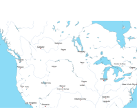
(a) $LD_{\mathrm{thr}}=2.5\%$, $LLDF=3.87\%$, $GLD=2.49\%$

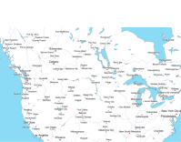
(b) $LD_{\mathrm{thr}}=12.5\%$, $LLDF=15.84\%$, $GLD=12.49\%$

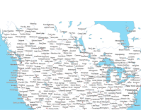
(c) $LD_{\mathrm{thr}}=100\%$, $LLDF=46.68\%$, $GLD=31.26\%$

Figure 5: Renders of map area 0 using PercepPPO at various values of $LD_{\mathrm{thr}}$ employed in label density experiment described in subsection 3.1.

We rendered the city labels in three different sizes as suggested by [16, 1, 12, 14] as more than three categories are perceived with difficulty, according to Robinson et al. [14]. As suggested by Tyner [19], we split the population into three intervals: ($<500,000$), (500,001–1,000,000), ($>1,000,000$), and apply three different font sizes of 11pt, 13pt, and 15pt, differing by 2pt as recommended by Robinson et al. [14].

We propose two different definitions of label density: (1) Local Label Density (LLD) and Global Label Density (GLD), typically expressed in percentages. We define LLD for each anchor $\alpha$ in map $M$, such that the anchor is the center of a tile $T$ of size $256\times 256$, which is the typical size of web-based raster maps. The LLD is defined as:

$$LLD(\alpha)=\frac{\sum_{a\in M}L(a)\cap T}{A(T)},$$ (3)

where $a$ is an anchor, $T$ is the square tile, $L(a)$ is the rectangle enclosing the label text corresponding to an anchor $a$, and $A(T)$ is the area of the tile. If the anchor is in the map $M$ positioned such that $T\cap M\neq T$, we perform a minimal shift of the tile $T$ to $M$ such $T\cap M=T$.

Similarly, we define GLD for each map $M$ as

$$GLD(M)=\frac{\sum_{a\in M}L(a)\cap M}{A(M)}.$$ (4)

We order the cities in the given map area by population size and process them iteratively. We sequentially try to add anchors and labels to the map, from the largest to the smallest. The anchor $\alpha$ is added to map $M$ at position $p$ from PPO if all of the following conditions are met: (1) $\alpha\in M$, (2) $L(\alpha)\cap M=L(\alpha)$, (3) $\forall a\in M,\,L(\alpha)\cap a=\emptyset$, (4) $\exists p\,\forall a\in M,\text{ such that }\alpha\neq a\,\land\,L(\alpha)\cap L(a)=\emptyset$, (5) $LLD(\alpha)\leq LD_{\mathrm{thr}}$, (6) $GLD(M)\leq LD_{\mathrm{thr}}$. After no other anchors can be labeled without conflict, we recompute the final $LLD$ ($LLDF$) for each placed anchor as we do not update $LLD(a_{1})$, when label $L(a_{2})$ protrudes from $T_{2}$ into $T_{1}$ and label $L(a_{2})$ is placed after $L(a_{1})$. Therefore, $LLDF$ can be slightly above $L_{\mathrm{thr}}$.

To prepare various samples of selected areas with different levels of label densities, we repeatedly rendered the area with $LD_{\mathrm{thr}}=(2.5\%-40\%,\mathrm{step\ size}\ 2.5\%)\cup(40\%,45\%,50\%,75\%,100\%)$. The upper part is more sparse because, with increasing levels of label density, the renders became perceptually similar. For example, only a few labels create differences between 40% and 42.5% or 50% and 55%. Therefore, we increased the step size to 5% from 40% and to 25% from 50%. If any rendered maps of a given area were the same, we kept only unique map renders. Following this procedure, we rendered ten selected areas (see Figure 5 and suppl. material) for selected PPOs from Tab. 1.

Verification

Additionally, we measured the number of positioned labels for all PPOs to ensure that anchors’ spatial configurations within selected areas do not discriminate against or favor a particular PPO. The 6(a) and 6(b) show that the number of placed labels is very similar for all PPOs.

(a) All $LD_{\mathrm{thr}}$ aggregated at $1305\times 1025$

(b) $LD_{\mathrm{thr}}=12.5\%$ at $1305\times 1025$

(c) $LD_{\mathrm{thr}}=12.5\%$ at $652\times 512$

Figure 6: 6(a) The box plot of placed labels for each examined PPO aggregated for all values of $LD_{\mathrm{thr}}$ at $1305\times 1025$. 6(b) The box plot of placed labels for label density $LD_{\mathrm{thr}}=12.5\%$ at $1305\times 1025$. 6(b) The box plot of placed labels for label density $LD_{\mathrm{thr}}=12.5\%$ at $652\times 512$.

Probabilities

Finally, we explored the adherence of label placements to their designated priorities and examined how increasing label densities influence the label placement. For each selected PPO outlined in Tab. 1, we have measured the probability of labels occupying specific positions and observed how these probabilities shift with escalating label densities.

As expected, labels are most likely to be positioned in their highest-priority position. The probability of the label being placed at the second highest priority was significantly lower, decreasing progressively for lower-priority positions (refer to Figure 7 and LABEL:fig:probabilities_density_all_methods in the suppl. material for insights into label density impacts). Nonetheless, some patterns deviated from this trend.

We observed a striking deviation with priorities of Imhof [9], where labels at lower densities were equally likely to occupy the second to fifth priority positions. However, as label density increased, this likelihood inverted, favoring lower-priority positions, realigning the priority sequence from the intended TR, R, T, B, L to TR, L, B, T, R for maps with greater label density. This density-dependent realignment in positioning probabilities is detailed in LABEL:fig:probabilities_density_all_methods in the suppl. material.

We also noted exceptions in the PPOs set by Slocum [16], Zoraster [26], and our PerceptPPO. For the priorities of Slocum, labels at higher densities are more likely to be placed at TL than at BR, contrary to the intended order BR, TL. Similarly, for the priorities of Zoraster, the likelihood of position BR is higher than for L or R, contrary to intended order R, L, BR. Likewise, PerceptPPO demonstrated a higher placement likelihood at L over TR or BR. The suppl. material further illustrates these individual probability patterns across different PPOs and their relation to label density in LABEL:fig:probabilities_density_all_methods.

Figure 7: The probability of a label being placed at a given position over all 30 locations rendered as described in subsubsection 3.1.1 with label density $LD_{\mathrm{thr}}=12.5\%$.

3.1.2 Procedure

Participants could access the study directly via a web application or indirectly via the Mechanical Turk interface, which embedded the same web app within its environment. The web application included an introduction, a survey, an experiment, and a feedback section. The introduction defined the participant’s task and how to use the application. Within the experiment, we presented rendered maps of selected areas in randomized order. Each participant was assigned a single PPO for all ten areas. Each participant was allowed to participate only once to mitigate the carry-over effect. For each area, we preloaded all renders with various label density levels. Using the slider, the participants were asked to ”choose a label density s/he finds comfortable without being overwhelmed by the amount of information.” The leftmost position was the lowest label density, and the rightmost position was the highest density. The participant must spend at least 5 seconds carefully selecting the preferred label density and explore the full range of label densities. When they complete all ten areas, we provide them the option to provide any feedback.

3.1.3 Results

We eliminated participants who exhibited inconsistencies within their responses across different areas and ones that deviated more than two standard deviations from the mean LLD and experiment duration, as described in subsection 2.4. After this data refinement, we engaged 110 participants from Mechanical Turk with a relatively high dropout of 45%, which we attribute to a spike of inattentive workers according to the review of activities recorded by Smartlook. Eliminated workers consistently set the slider in the right or leftmost position, which is highly unlikely to be the preferred position according to the control group. We found that the preferred median for $LD_{\mathrm{thr}}$ is $12.5\%$ ($\bar{x}=14.85\%$, $SD=7.22\%$), corresponding to median $LLDF$ of $16\%$ ($\bar{x}=17\%$, $SD=7.35\%$), median $GLD$ of $12.5\%$ ($\bar{x}=14.54\%$, $SD=6.59\%$) and 150 labeled anchors on median ($\bar{x}=159$, $SD=82$).

Upon conducting an Analysis of Variance (ANOVA) to investigate the effect of different PPOs on the $LD_{\mathrm{thr}}$, our results indicated no significant differences across the various PPOs. Specifically, the ANOVA test, utilizing a Type II sum of squares approach, yielded an F-statistic of $1.660$ with a corresponding $p$-value of $0.127$. The $p$-value suggests that we found no statistically significant differences in $LD_{\mathrm{thr}}$ values among PPOs at significance level $\alpha=0.05$.

The finding implies that the examined PPOs do not significantly affect the $LD_{\mathrm{thr}}$ value, reinforcing the idea that the variations observed in $LD_{\mathrm{thr}}$ across different PPOs might be attributed to random chance rather than inherent differences in PPOs. Therefore, our analysis supports the conclusion that the selection of PPOs does not significantly influence the $LD_{\mathrm{thr}}$.

3.2 Experiment 2: Comparison of PPOs

To compare the proposed PerceptPPO with existing PPOs, we conducted an experiment that follows findings from the label density experiment described in subsection 3.1. We aim to validate that the PerceptPPO is preferred when the label cannot always be placed in a single position (see Figure 8), unlike the PerceptPPO experiment described in section 2.

3.2.1 Data

In this experiment, we are employing the same approach as described in subsubsection 3.1.1 with $LD_{\mathrm{thr}}=12.5\%$, but this time, we reduced the size of renders to half $652\times 512$ which means that the median number of shown anchors and labels is 26 ($\bar{x}=24.79$, $SD=5.91$), contrary to 131.5 ($\bar{x}=131.31$, $SD=21.01$) for $1305\times 1025$, see Figure 6 and suppl. material. We found out that comparing map pairs with 131.31 labels on average is overly demanding and cannot be completed in a reasonable time. Therefore, we chose to reduce the size of the map area while still maintaining the $LD_{\mathrm{thr}}=12.5\%$ but with 24.79 presented labels on average, see Figure 8. In this experiment, we also use all 30 locations worldwide as described in subsection 2.1. Other data characteristics hold with subsubsection 3.1.1, except the background is blank as in subsection 2.1.

Verification

Again, we measured the number of placed labels for all PPOs to ensure that anchors’ spatial configurations within selected areas do not discriminate against or favor a particular PPO. The 6(c) show that the number of placed labels is very similar for all PPOs.

Probabilities

Finally, we explored the adherence of label placements to their designated priorities for the data used in the experiment ($652\times 512$ size of renders at $LD_{\mathrm{thr}}=12.5\%$), see LABEL:fig:probabilities_density_all_methods_2 in the suppl. material. We found the same deviations for the priority orders of Imhof, Zoraster, and PerceptPPO as for the data with $1305\times 1025$ size of renders at $LD_{\mathrm{thr}}=12.5\%$ (see subsubsection 3.1.1).

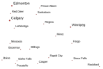
(a) Brewer

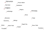
(b) Christensen

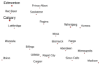
(c) Zoraster

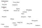
(d) PerceptPPO

Figure 8: Renders of map area 0 using various PPOs at $LD_{\mathrm{thr}}=12.5\%$ employed in comparison of PPOs described in subsection 3.2.

3.2.2 Procedure

We applied the 2AFC paradigm to determine the preferred PPO based on the perception of users. Considering the seven PPOs under examination, we have ${{7}\choose{2}}=21$ pairwise comparisons on an area. Consequently, the entire experiment consists of $30\times 21=630$ pairwise comparisons to cover all of them once. In order to alleviate potential fatigue among the participants during the study, we allocated only three areas to each participant, resulting in a batch of $3\times 21=63$ pairwise comparisons. Therefore, 10 participants were required to cover all pairwise comparisons once. We engaged Mechanical Turk workers and university students to perform the experiment. The rest of the procedure is the same as for subsection 2.2 except, participants were shown two maps sequentially, each depicting the same area but with different PPOs.

3.2.3 Results

We eliminated participants with inconsistent responses as described in subsection 2.4. Following this data refinement, we were left with a total of 352 participants with a dropout of 24%. These participants generated 22,236 pairwise comparisons. Therefore, on average, each comparison pair was evaluated by approximately 35 different participants.

The overall median of consistency $\zeta$ across participants is 0.57 ($\bar{x}=0.59$, $SD=0.23$), which indicates that they were fairly consistent in their choices. The consistency remained reasonably uniform across each map area; details are provided in LABEL:tab:ppo-eval-results in the suppl. material. However, the overall coefficient of agreement $u=0.013$ ($\mathrm{min}\ u=-0.0009$) reveals relatively low agreement among participants, although the $p$-value $=7.362e^{-55}$ clearly shows that we can reject the null hypothesis $H_{0}^{2}$: “There is no agreement among participants” at $\alpha=0.05$ and conclude there is indeed some agreement.

Using hierarchical clustering applying Ward’s minimum variance method, we identified three participant clusters as shown in Figure 9. Even though for individual areas, the $p$-value is sometimes greater than $\alpha=0.05$, which disallows us to reject the null hypothesis $H_{0}^{2}$ for individual areas, aggregation of the preference matrices over all areas leads to $p$-values lower than $\alpha=0.05$ for all clusters. Therefore, among all clusters, there was some agreement among participants. Detailed results supporting found clustering, including statistics and cluster compositions, can be found in LABEL:tab:ppo-eval-results in the suppl. material.

Cluster 1 ($N=134$) depicted in 9(a) with mean consistency $\zeta_{1}=0.659$ $(SD=0.232,Q2=0.714)$ shows fairly high agreement $u_{1}=0.218$ ($\mathrm{min}\ u_{1}=-0.002$, $p$-value$=0$) and contains participants that prefer PPOs in group $G_{T}=\{\texttt{PerceptPPO},\texttt{Zoraster}\}$. Cluster 2 ($N=82$) shown in 9(b) with mean consistency $\zeta_{2}=0.612$ $(SD=0.223,Q2=0.643)$ and slightly lower agreement $u_{2}=0.131$ ($\mathrm{min}\ u_{2}=-0.004$, $p$-value$=1.25e^{-134}$), comprises participants that prefer PPOs in group $G_{TR}=\{\texttt{Brewer},\texttt{YoeliB},\texttt{Christensen},\texttt{Slocum},\texttt{Imhof}\}$ contrary to $G_{\mathrm{T}}$. Cluster 3 ($N=136$) presented in 9(c) with mean consistency $\zeta_{3}=0.502$ $(SD=0.210,Q2=0.500)$ and relatively low agreement $u_{3}=0.005$ ($\mathrm{min}\ u_{3}=-0.002$, $p$-value$=7.63e{-6}$) includes participants that are uncertain in their preferences but slightly incline towards $G_{\mathrm{T}}$ over $G_{\mathrm{TR}}$.

(a) C1 ($N=134$, $\zeta_{1}=0.659$, $u_{1}=0.218$, $p=0$)

(b) C2 ($N=82$, $\zeta_{2}=0.612$, $u_{2}=0.131$, $p=1.2e^{-134}$)

(c) C3 ($N=136$, $\zeta_{3}=0.502$, $u_{3}=0.005,p=7.6e^{-6}$)

Figure 9: Identified clusters of users in a comparison study of PPOs with depicted quality z-scores and 95% confidence intervals. The red dashed brackets, with the corresponding $p$-values reported above, represent the PPOs pairs without evidence of statistically significant differences at $\alpha=0.05$ using the two-tail test. Conversely, between the PPOs pairs without brackets are detected statistically significant differences.

We apply methodology as described in subsubsection 2.3.3 to compute the quality z-score and assess statistical significance at the significance level of $\alpha=0.05$ to evaluate the null hypothesis $H_{0}^{3}$: “There is no clear user preference among the examined PPOs.”

The overall results, as depicted in Figure 10, show a statistically significant difference between PPO groups $G_{T}=${PerceptPPO, Zoraster} and $G_{TR}=${Brewer, YoeliB, Christensen, Slocum, Imhof}. However, results also show no significant difference in user preference within these PPO groups. Therefore, we can reject the null hypothesis $H_{0}^{3}$ and claim that there is a clear preference of PPOs only between groups $G_{\mathrm{T}}$ and $G_{\mathrm{TR}}$. In other words, participants perceived PPOs in $G_{\mathrm{T}}$ significantly better than in $G_{\mathrm{TR}}$. The outcome validates the findings of our PercepPPO study described in section 2 that participants prefer label position $T$ at the first place of PPO as proposed by Zoraster and PerceptPPO. Interestingly, the results also imply that second place in PPO is not that important. Therefore, participants prefer labels mostly centered above the anchor, but the following positions do not seem essential for perceiving the quality of PPOs.

In this experiment, we engaged 352 participants comprising of 179 females and 173 males. A majority of the participants hailed from the USA (221), followed by India (54), Czech Republic (32), Brazil (7), United Kingdom (5). The most common age range among the participants was 20-30 years, with 98 individuals falling into this category, followed by 31-40 with 93 participants, 41-50 with 77 participants, 51-60 with 47 participants, $>60$ with 35 participants and 2 participants bellow 20. Regarding educational qualifications, the highest number of participants held bachelor’s degrees (163), master’s degrees (76), followed by high school diplomas (67), community college education (38), doctoral’s degrees (7), and elementary education (1). On average, participants completed a batch of 63 pairwise comparisons in 10 minutes and 46 seconds ($SD=$ 3 minutes and 13 seconds).

Figure 10: Overall comparison of PPOs. Chart 10 depicts quality score and 95% confidence intervals. Chart 10 shows the statistical significance with $p$-values in brackets. Statistically significant differences between pairs of PPOs are denoted by solid blue lines. Conversely, red dashed lines represent pairs of PPOs without evidence of statistically significant differences.

4 Discussion

The PerceptPPO study showcases the potential of a user-centered approach to enhancing the principles of label placement in cartography and GIS. The high consistency observed among the participants, with an overall median of 0.75 and a mean of 0.67, underscores the reliability of user judgments in determining the perceptual preference order of label positions around point features. Notably, the study established a clear overall preference order: top (T) $>$ bottom (B) $>$ right (R) $>$ top-right (TR) $>$ bottom-right (BR) $>$ left (L) $>$ top-left (TL) $>$ bottom-left (BL). This finding challenges traditional conventions and suggests a shift towards prioritizing labels above or bellow of point features for improved user experience.

The experiment on label density offers a brief view into how users perceive and prefer the density of labels on maps—the average preferred Local Label Density (LLDF) of 17% reflects the preferred label density in the local region of a map. The average Global Label Density of 14.5% suggests that users favor a moderate label presence, enough to inform without being too crowded. The balance is crucial for creating user-friendly maps that facilitate easy navigation and understanding.

Finally, the comparison between PerceptPPO and existing PPOs reveals that PerceptPPO’s perceived quality surpasses that of traditional PPOs and aligns closely with Zoraster. Although the $p$-value is close to $\alpha$, the difference in quality is not statistically significant when using the two-tail test. This outcome suggests that the initial position within a PPO plays a crucial role in its perceived effectiveness, with subsequent positions having less impact on overall user perception.

5 Limitations

While the study presents a statistically significant ordering of label positions, it also uncovers distinct clusters of user preferences, revealing the complexity of perceptual prioritization. We used generic blind maps that, on the one hand, minimize the degree of freedom and enable precise evaluation of preferences, but on the other hand, it is essential to acknowledge that other elements of a map could also influence user perception. Additionally, this study did not account for semantic considerations – such as the placement of city labels across state borders or the positioning of coastal city labels towards water bodies, as highlighted by Imhof [9]. Preferences might also vary based on the map’s intended use and audience, from military to recreational purposes. The demographic aspects may similarly affect the preferences for languages with right-to-left or top-to-bottom scripts. Notably, the study did not delve into the functional aspect of label placement, including ease of information search and overall readability, which are critical for user engagement with the map. Despite stringent participant screening and measures to ensure data integrity, the inherent variables associated with the uncontrolled online environment could introduce unseen biases.

The outcomes of our study lay a solid foundation, yet further research is needed to explore the aforementioned factors. Future work should investigate how semantic rules, map purpose, target audience preferences, and functional aspects such as readability interplay with the perceptual prioritization of label positions to develop more nuanced guidelines for map design.

6 Conclusion

In this work, we introduced Perceptual Position Priority Order (PerceptPPO), fundamentally reviewing the point-feature label placement by prioritizing user preferences over traditional conventions. Engaging nearly 800 participants globally, we have established a user-preferred ordering of label positions along the feature point that challenges and diverges from the conventional top-right towards the top position. Moreover, we performed an additional study to find users’ preferred label density, a domain narrowly studied in prior literature. According to the results, users prefer, on average, 17% of the generic map to be covered by labels. Finally, the comparative analysis underscores PerceptPPO’s superiority in perceived quality against traditional PPOs, particularly highlighting the significance of the first label position’s role in user perception. Our empirical study marks a significant step toward more intuitive and user-centered map designs, emphasizing the importance of aligning label placement visualization practices with actual user expectations.

- [1] C. Brewer. Designing better maps: a guide for GIS users. ESRI Press, 2 ed., 2015.
- [2] B. Chazelle and N. Amenta. Application challenges to computational geometry. Technical Report TR-521-96, Computational Geometry Impact Task Force, 1999.
- [3] J. Christensen and J. Marks. An empirical study of algorithms for point-feature label placement. ACM Transactions on Graphics, 14:203–232, 1995.
- [4] H. A. David. The method of paired comparisons. Oxford University Press, 2nd ed., 1988.
- [5] D. B. Dent, J. S. Torguson, and T. W. Hodler. Cartography: Thematic Map Design. McGraw-Hill Education, 6 ed., 2009.
- [6] L. R. Ebinger and A. M. Goulette. Automated names placement in a non-interactive environment. In Auto-Carto IX, Proceedings of the International Symposium on Computer-Assisted Cartography, pp. 205–214, 1989.
- [7] W. D. Hua Liao, Xueyuan Wang and L. Meng. Measuring the influence of map label density on perceived complexity: a user study using eye tracking. Cartography and Geographic Information Science, 46(3):210–227, 2019. doi: 10 . 1080/15230406 . 2018 . 1434016
- [8] E. Imhof. Die anordnung der namen in der karte. International Yearbook of Cartography, 2:93–129, 1962.
- [9] E. Imhof. Positioning names on maps. American Cartographer, 2(2):128–144, 1975. doi: 10 . 1559/152304075784313304
- [10] C. B. Jones. Cartographic name placement with prolog. IEEE Computer Graphics and Applications, 9:36–47, 1989. doi: 10 . 1109/38 . 35536
- [11] M. G. Kendall and B. Smith. On the method of paired comparisons. Biometrika, 34:363–365, 1947. doi: 10 . 1093/biomet/34 . 3-4 . 363
- [12] J. Krygier and D. Wood. Making maps: a visual guide to map design for GIS. Guilford Publications, 3 ed., 2016.
- [13] M. Pérez-Ortiz and R. K. Mantiuk. A practical guide and software for analysing pairwise comparison experiments. Technical report, 2017.
- [14] A. H. Robinson, J. Morrison, P. Muehrcke, A. Kimerling, and S. Guptill. Elements of Cartography. Wiley, 6 ed., 1995.
- [15] J. Scheuerman, J. L. Harman, R. R. Goldstein, D. Acklin, and C. J. Michael. Visual preferences in map label placement. Discover Psychology, 3:27, 2023. doi: 10 . 1007/s44202-023-00088-0
- [16] T. A. Slocum, R. B. McMaster, F. C. Kessler, and H. H. Howard. Thematic Cartography and Geovisualization. Pearson, 3 ed., 2009.
- [17] L. L. Thurstone. A law of comparative judgment. Psychological Review, 34:273–286, 1927.
- [18] K. Tsukida and M. R. Gupta. How to Analyze Paired Comparison Data. UWEE Technical Report 206, 2011.
- [19] J. A. Tyner. Principles of map design. Guilford Publications, 2014.
- [20] F. Wickelmaier and C. Schmid. A Matlab function to estimate choice model parameters from paired-comparison data. Behavior Research Methods, Instruments, and Computers, 36(1):29–40, 2004. doi: 10 . 3758/BF03195547
- [21] C. H. Wood. A descriptive and illustrated guide for type placement on small scale maps. Cartographic Journal, 37:5–18, 2000. doi: 10 . 1179/caj . 2000 . 37 . 1 . 5
- [22] M. Yamamoto, G. Camara, and L. A. N. Lorena. Fast point-feature label placement algorithm for real time screen maps. In GEOINFO 2005 - 7th Brazilian Symposium on GeoInformatics, 2005.
- [23] P. Yoeli. The Logic of Automated Map Lettering. The Cartographic Journal, 9(2):99–108, 1972. doi: 10 . 1179/000870472787352505
- [24] S. ZORASTER. Integer programming applied to the map label placement problem. Cartographica: The International Journal for Geographic Information and Geovisualization, 23(3):16–27, 1986. doi: 10 . 3138/9258-63QL-3988-110H
- [25] S. Zoraster. Solution of large 0-1 integer programming problems encountered in automated cartography. Operations Research, 38:752–759, 1990. doi: 10 . 1287/opre . 38 . 5 . 752
- [26] S. Zoraster. Practical results using simulated annealing for point feature label placement. Cartography and Geographic Information Systems, 24(4):228–238, 1997. doi: 10 . 1559/152304097782439259