PECCARY: A novel approach for characterizing orbital complexity, stochasticity, and regularity

Abstract

Permutation Entropy and statistiCal Complexity Analysis for astRophYsics (PECCARY) is a computationally inexpensive, statistical method by which any time-series can be characterized as predominately regular, complex, or stochastic. Elements of the PECCARY method have been used in a variety of physical, biological, economic, and mathematical scenarios, but have not yet gained traction in the astrophysical community. This study introduces the PECCARY technique with the specific aims to motivate its use in and optimize it for the analysis of astrophysical orbital systems. PECCARY works by decomposing a time-dependent measure, such as the x-coordinate or orbital angular momentum time-series, into ordinal patterns. Due to its unique approach and statistical nature, PECCARY is well-suited for detecting preferred and forbidden patterns (a signature of chaos), even when the chaotic behavior is short-lived or when working with a relatively short duration time-seriesor small sets of time-series data. A variety of examples are used to demonstrate the capabilities of PECCARY. These include mathematical examples (sine waves, varieties of noise, sums of sine waves, well-known chaotic functions), a double pendulum system, and astrophysical tracer particle simulations with potentials of varying intricacies. Since the adopted timescale used to diagnose a given time-series can affect the outcome, a method is presented to identify an ideal sampling scheme, constrained by the overall duration and the natural timescale of the system. The accompanying PECCARY Python package and its usage are discussed.

1 Introduction

Permutation Entropy and statistiCal Complexity Analysis for astRophYsics (PECCARY) is a statistical method used to characterize a time-series as regular, stochastic (i.e., random or noisy), or complex, and identify its relevant timescales (Bandt & Pompe, 2002; Rosso et al., 2007; Weck et al., 2015). The use of Permutation Entropy and Statistical Complexity measures has been gaining traction in a wide variety of physical, biological, and mathematical scenarios, including plasma turbulence (Maggs & Morales, 2013; Gekelman et al., 2014; Weck et al., 2015; Maggs et al., 2015; Zhu et al., 2017), Solar wind and space plasma (Suyal et al., 2012; Weck et al., 2015; Ribeiro et al., 2017; Olivier et al., 2019; Weygand & Kivelson, 2019; Good et al., 2020), geological processes (Donner et al., 2015), river flow (Serinaldi et al., 2014; Thaxton et al., 2018), economic trends (Zunino et al., 2010; Bariviera et al., 2013; Araujo et al., 2020), biological or medical rhythms (Jordan et al., 2008; Li et al., 2010; Aronis et al., 2018), and for understanding the spread of the COVID-19 virus (Fernandes et al., 2020).

One of the drivers of the evolution of a dynamical orbital system depends on the relative fraction and distribution of regular and complex orbits, as well as the timescales associated with each. Indeed, the formulation of chaos theory itself is firmly rooted in the study of chaotic behavior in astrophysical dynamical systems (e.g., the three body problem, Poincaré, 1891) and continues to inform studies of the secular evolution of galaxies (e.g., Fux, 2001; Pichardo et al., 2003; Patsis, 2006; Manos & Athanassoula, 2011; Valluri et al., 2016), planetary systems (e.g., Malhotra, 1993; Gladman, 1993; Saha & Tremaine, 1993; Astakhov et al., 2003; Lithwick & Wu, 2011; Deck et al., 2013), and black hole dynamics (e.g., Contopoulos, 1990; Suzuki & Maeda, 2000; Merritt & Poon, 2004), to name a few. The role of chaos in the evolution of dynamical systems is not the same as that of stochastic processes (whether physical or computationally induced, see Pfenniger, 1986; Kandrup & Willmes, 1994; Murray-Clay & Chiang, 2006; Sellwood & Debattista, 2009; Neyrinck et al., 2022, for various treatments), though they can be nearly indistinguishable in practice (Rosso et al., 2007) and quite often both are confusingly labeled “stochastic.” Differentiating between the two is particularly relevant in understanding the difference between dynamical processes and issues that arise from the limited resolution in discretized computation, like shot noise (e.g., Schaap & van de Weygaert, 2000; Dehnen, 2001; Varadi et al., 2003; Sellwood & Debattista, 2009; Sellwood, 2014).

The PECCARY method is able to discern the nature of fluctuations in a time-series through its decomposition into a distribution of the occurrence frequency of patterns (described in Section 2.1). PECCARY can be set apart from well-known methods for determining regions of orbital chaos or irregularity, such as Lyapanov exponential divergence (e.g., Pichardo et al., 2003), Kolmogorov-Arnold-Moser (KAM) theory analysis (Weinberg, 2015a, b), Frequency Map Analysis (e.g., Laskar et al., 1992; Papaphilippou & Laskar, 1996, 1998; Valluri & Merritt, 1998; Valluri et al., 2012; Price-Whelan et al., 2016; Beraldo e Silva et al., 2019), and Surface of Section (SoS) analysis (e.g. Martinet, 1974; Athanassoula et al., 1983) since it is optimized to identify chaotic behavior on relatively short timescales and is agnostic to underlying physics. PECCARY expands the toolbox that astrophysical researchers have at their disposal for understanding dynamical systems. It provides an analysis technique that is suitable in situations where long-standing traditional techniques may not be as applicable, such as simulations with time-dependent potentials (e.g., a slowing bar or in systems that are accreting mass).

This work introduces the theoretical framework of PECCARY and explores its applicability and limitations in astrophysical systems. §2 gives an overview of the theory, how ordinal patterns are determined, how the metrics of Permutation Entropy and Statistical Complexity are computed, and the usage of the $HC$-plane. §3 discusses the usage, interpretation, and limitations of the method, as well as an idealized sampling scheme. §4 demonstrates the capabilities of PECCARY via a variety of mathematical, physical, and astrophysical examples. §5 provides an outlook into future work and tests to be done with PECCARY, and §6 summarizes the conclusions.

2 Overview of the PECCARY Method

PECCARY is comprised of two different statistical measures: Permutation Entropy and Statistical Complexity. The Permutation Entropy and Statistical Complexity measures were developed in the early 2000s (e.g., Bandt & Pompe, 2002; Rosso et al., 2007) as a way to distinguish noise from discrete chaotic maps, such as the logistic map or bifurcation diagram.

In this context , PECCARY uses a discretized time-series through a sampling scheme (described in Section 2.1) and calculates the Permutation Entropy and Statistical Complexity values in order to determine what type of behavior (regular, stochastic, complex) is exhibited. This is done by extracting and counting the occurrence frequency of the sampled data, which are called “ordinal patterns.” Ordinal patterns are groups of points that are ordered from smallest to largest relative amplitude. The resulting order of indices is that ordinal pattern. For example, if a series of points had values [8, 3, -2, 5] the resulting pattern would be “3241” since the third value of the array is the smallest, the second one is the second smallest, etc. Section 2.1 gives a more in-depth discussion of how these ordinal patterns are extracted and determined.

PECCARY operates on the principle that ordinal patterns may be found within any time-series that has $N$ discrete, sequential measurements, calculations, or simulated quantities taken at fixed separation. Since the ordinal patterns are determined purely by comparing relative amplitudes, PECCARY is agnostic to the physics and other parameters of the system (which often factor into other chaos/noise differentiation methods).

2.1 Determination of Ordinal Patterns

In their pioneering work, Bandt & Pompe (2002) developed the Permutation Entropy ($H$) measure as a means to identify chaotic behavior. Their approach relied on what they called “ordinal patterns.” An ordinal pattern is defined as the order in which a subset of $n$ sequential, discrete measurements from a given time-series appears such that their values increase from lowest relative amplitude to highest relative amplitude. In cases where there exist two equal values, the original order of points in the time-series is preserved. The values themselves are irrelevant since the magnitude of change between steps plays no role in this analysis.

Figures 1 and 2 illustrate this definition. In Figure 1(a), a set of $N=19$ points is shown representing an arbitrary time-series along the horizontal axis. The three shaded regions highlight sets of $n=5$ time-steps, which in this case are both sequential and contiguous. These sequences are again shown in Figures 1(b), (c), and (d), with the ordinal pattern written at the bottom of each panel. The ordinal pattern for these sets of five points is found by first determining which ordinal position has the lowest value, then which ordinal position has the next lowest value, and so on through each of the five points. This pattern can be represented by the numerical sequence shown at the bottom of each of the lower panels in Figure 1.

Ordinal patterns are extracted through a method that uses two parameters: the sampling size $n$ and the sampling interval $\ell$. The sampling size $n$ is the number of sequential points extracted to construct the ordinal patterns. Any time-series can be decomposed into consecutive, overlapping sets of $n$ time-steps, where the number of possible permutation orders is $n!$. The sampling interval $\ell$ is the integer number of timesteps from one sampled point to the next and probes the corresponding physical timescale in PECCARY (e.g., Zunino et al., 2012; Gekelman et al., 2014; Weck et al., 2015). The timescale for an extracted ordinal pattern associated with a given sampling size and sampling interval (known as the “pattern timescale”) is given by,

$$t_{\rm pat}=\ell\,\delta t(n-1)\;,$$ (1)

where $\delta t$ is the time-step resolution and the pattern length spans $n-1$ sampling intervals $\ell$.

The sampling interval for consecutive points is given by $\ell=1$. It is not necessary, and often not optimal, for the $n$ extracted time-steps used to construct an ordinal pattern be contiguous (i.e., $\ell=1$). Figure 2 illustrates how ordinal patterns using sampling interval $\ell=3$ are constructed using the same pattern from Figure 1. Here, every third point is grouped as shown by a given color. These three sets of five points are shown in panels (b)-(d) in Figure 2 and the numerical representation of their ordinal patterns are also indicated, as in Figure 1.

Note that Bandt & Pompe (2002) called the sampling size the “embedding dimension” and the sampling interval the “embedding delay.” These refer to the same parameters, but this paper adopts different language for a more intuitive framing.

In order for PECCARY to produce meaningful results, the sampling size $n$ must be large enough that the set of possible ordinal patterns can be robustly used to describe the time-series ($n{>}2$, Bandt & Pompe, 2002), but not so large that the number of patterns becomes intractable. To the second point, PECCARY requires the condition $n!\ll N$ be met, where $N$ is the total number of sequential points in the time-series (Rosso et al., 2007). Bandt & Pompe (2002) noted that a practical choice lies between $3\leq n\leq 7$. They did not attempt a thorough proof; rather, they showed that chaotic behavior is well identified (even for noisy data) using values of $n$ within these bounds, with a slightly clearer signal near $n=6$. A sampling size of $n=5$ is adopted throughout this study, following the practice of several studies that effectively use Permutation Entropy (e.g., Cao et al., 2004; Rosso et al., 2007; Weck et al., 2015). A more thorough theoretical treatment is beyond the scope of this work but would yield useful justification for one’s choice of $n$ in future studies.

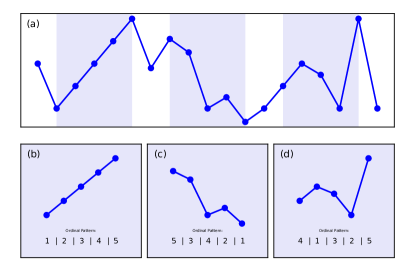
Figure 1: An arbitrary time-series of $N=19$ discrete points used to construct embedding dimension $n=5$ ordinal patterns. Shaded regions in panel (a) indicate three examples of patterns using sampling interval $\ell=1$. Shaded points in panels (b)-(d) show the ordinal pattern from lowest value (bottom) to highest value (top) of the five points within each shaded region. This ordinal pattern can be represented by the numerical sequence listed at the bottom of each panel.

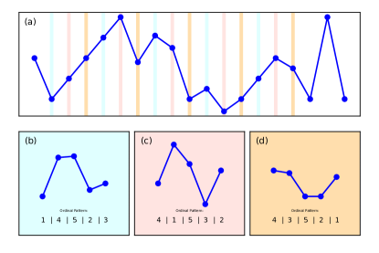
Figure 2: The same arbitrary time-series of $N=19$ discrete points from Figure 1, but with color coded shading corresponding to embedding dimension $\ell=3$ (i.e., skipping every two time-steps). Each highlighted pattern is projected in panels in (b)-(d) to illustrate the ordinal pattern extracted from the $\ell=3$ sampling. The ordinal patterns extracted using $\ell=3$ are different than those using $\ell=1$ in Figure 1.

2.2 Pattern Probability and Pattern Probability Distributions

After extracting the $\ell(n-1)$ ordinal patterns from the time-series, the pattern probability distribution $P$ (also called the “pattern distribution” by Weck et al. (2015)) can be produced for the $n!$ possible patterns. The probability $p(\pi_{i})$ for each pattern $\pi_{i}$ in $P$ is found by normalizing the occurrence frequency of that pattern so that

$$\sum_{i}^{n!}p(\pi_{i})=1\;,$$ (2)

where the subscript $i$ denotes one of the $n!$ possible patterns. The nature of a time-series as regular, stochastic, or complex, can be discerned by calculating two statistical measures, the Permutation Entropy $H$ and Statistical Complexity $C$ of the resulting pattern probability distribution $P$, for a given sampling size $n$ and sampling interval $\ell$. Section 2.3 introduces and describes these measures in depth.

It is useful to consider the following two extreme cases: (1) a distribution where every pattern is equally represented (e.g., white noise), as in Figure 3(a), and (2) a periodic time-series dominated by very regular patterns (e.g., a sine wave), as visualized by a histogram of the occurrence frequency in Figure 3(c). Most distributions have a more complex set of occurrence frequencies, as exemplified by the distribution in Figure 3(c). Such distributions reveal favored (high occurrence frequency) or forbidden patterns (low or zero occurrence frequency).

Time-series data analyzed using PECCARY must adequately populate the $n!$ patterns in order to ensure the value for each occurrence probability $p(\pi_{i})$ is statistically significant. In practice, either the time-series must be sufficiently long or multiple time-series can be combined. The first case is appropriate for long datasets where the characteristic behavior of the time-series is not time-dependent, as in the case study in §4.2. The latter is appropriate for shorter characteristic timescales and requires an ensemble of time-series. In any case, PECCARY is only able to probe the characteristic behavior of a time-series at timescales corresponding to an appropriately sampled time domain. Section 3.2 discusses a method for determining the minimum time-series duration as well as a range of appropriate sampling intervals.

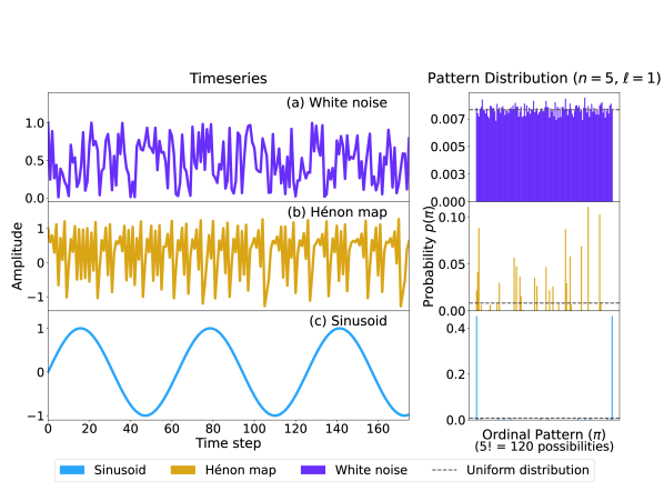
Figure 3: Left: Sample section of time-series from $t=0$ to $t=175$ out of $t=0$ to $t=5\times 10^{4}$ for (a) white noise (stochastic), (b) Hénon Map (chaotic), and (c) sinusoidal (periodic), where the inset is a zoom-in of a short timescale segment of the series. Right: Ordinal pattern probability $p(\pi)$ for possible ordinal patterns $\pi$ for each time-series given an sampling size $n=5$ and sampling interval $\ell=1$. The stochastic time-series has a uniform distribution of patterns, the periodic time-series has a small number of preferred patterns, and the chaotic time-series has a variety of preferred, underpreferred, and forbidden patterns.

2.3 Permutation Entropy and Statistical Complexity

The core of the PECCARY method is the calculation of the Permutation Entropy and Statistical Complexity, which are used in combination to evaluate whether a given time-series is regular, complex, or stochastic. Table 1 provides a glossary of the terms used in this section, as well as equation references.

2.3.1 Permutation Entropy

A common metric for a pattern probability distribution $P$ is the Shannon Entropy (or information entropy) (Shannon, 1948), expressed as,

$$S[P]=-\sum_{i}^{n!}p(\pi_{i})\log p(\pi_{i})\;.$$ (3)

The value of $S$ normalized to its maximum possible value, i.e.,

$$H[P]=\dfrac{S[P]}{\log n!},$$ (4)

is the Permutation Entropy (Bandt & Pompe, 2002; Rosso et al., 2007). Using this metric, a time-series that is dominated by a single pattern (e.g., a linear ramp), would have $H=0$, while an equally probable distribution of patterns (e.g., white noise, as in Figure 3(a)), would have $H=1$. An intermediate pattern, as in Figure 3(b), would have an intermediate value for $H$.

Periodic time-series, such as sine waves or triangle waves, have limited numbers of possible permutations, as in Figure 3(c). There are upward and downward ordered ramp patterns and some additional patterns from permutations that include local maxima or minima in the periodic function.

The number of possible patterns does not change with embedding delay since the same patterns are possible no matter the sampling resolution. However, the probability for a given pattern does depend on the sampling resolution. For example, the probability for ramp patterns increases as the sampling interval decreases.

The lower limit for the value of $H$ for a periodic function is the limit when only two ramping patterns (upward and downward) are measured. That is,

$$H_{\rm per}^{\rm min}(n)=\frac{\log 2}{\log(n!)}.$$ (5)

The limiting minimum possible value for the Permutation Entropy of a periodic function when $n=5$ is thus $H_{\rm per}^{\rm min}(n{=}5)=0.14478$.

The limiting maximum possible value of $H$ for a periodic function is the case when the probability of each possible pattern is equal. The number of possible patterns for any periodic function composed of two ramping patterns is conjectured to be

$$N_{\rm periodic}(n)=2[2(n-2)+1].$$ (6)

This can be understood in the case of a triangle function. There is one upward ramping pattern (last term in brackets), and there are $(n-2)$ non-ramp patterns around the crest where any evenly spaced sampling will either have points sampled on the right side staggered with higher than values than on the left or vice versa (second term in brackets). There is also a symmetry for downward ramping points and points around the trough. The same ordinal patterns exist for single-frequency periodic functions, like sine and cosine, which are indistinguishable from a triangle function with the same maximum/minimum frequency. This hypothesis has been tested for the range of sampling sizes between $3<n<8$. It follows that,

$$H_{\rm per}^{\rm max}(n)=\frac{\log N_{\rm periodic}(n)}{\log(n!)}.$$ (7)

Since $N_{\rm periodic}(n{=}5)=14$, a periodic function sampled with an sampling size of $n{=}5$ is expected to have $H{\leq}H_{\rm per}^{\rm max}{=}0.55124$.

2.3.2 Disequilibrium and Complexity

The pattern probability distribution $P$ can also be characterized by how poorly it is described by the pattern probability distribution for the uniform case, $P_{e}$, where each possible pattern has equal probability $p_{e}=1/n!$. The divergence of ensemble $P$ from $P_{e}$ is called the “disequilibrium” and is defined as,

$$d[P,P_{e}]=S\left[\frac{P+P_{e}}{2}\right]-\frac{1}{2}S[P]-\frac{1}{2}S[P_{e}]\;,$$ (8)

where $S[P+P_{e}]$ is the Shannon Entropy for the sum of pattern probability distributions $P$ and $P_{e}$. The value of the disequilibrium $d(P,P_{e})$ is normalized by its maximum possible value ($d/d_{\rm max}$) is given by (Lamberti et al., 2004),

$$D[P,P_{e}]=\dfrac{2d[P,P_{e}]}{2\log(2n!)-\log(n!)-\frac{n!+1}{n!}\log(n!+1)}\;,$$ (9)

and scales in the opposite direction to the Permutation Entropy (e.g., $D\rightarrow 1$ as $H\rightarrow 0$). Statistical Complexity, also known as the Jensen-Shannon Complexity, is given by the product (Lamberti et al., 2004; Rosso et al., 2007),

$$C[P,P_{e}]=D[P,P_{e}]\,H[P].$$ (10)

Low values for $C$ indicate a system with a distribution of ordinal patterns that are either far from the uniform distribution, as $H$ approaches zero, or very near the uniform distribution, as $D$ approaches zero. Maximum complexity occurs in an intermediate range when both $H$ and $D$ are non-zero.

The Statistical Complexity ($C$) measure has been compared to several established (e.g., Lyapanov analysis) and emerging (e.g., the LMC measure López-Ruiz et al., 1995) methods for identifying chaotic or complex behavior and is shown to be robust for a wide range of scenarios (Lamberti et al., 2004; Rosso et al., 2007), including logistic maps, the skew tent map, the Hénon map, the Lorenz map of Rossler’s oscillator, and Schuster maps (Schuster, 1988). Further, $C$ is an intensive measure that can be used to provide insight into the dynamics of a system (Lamberti et al., 2004), such as relevant timescales (explored in Sections 2.4 & 4). It is also reliably able to quantify the degree of chaos in systems that also have some degree of periodicity (Lamberti et al., 2004) or stochasticity (Rosso et al., 2007; Zunino et al., 2012).

Table 1: Glossary of Statistical Terms

Symbol	Name	Definition	Eq. no
P	Pattern probability distribution	All possible $n!$ ordinal pattern permutations	§2.2
P_e	Equilibrium pattern probability distribution	Uniform distribution of all possible $n!$ ordinal pattern permutations	§2.3.2
π_i	i-th ordinal pattern	A possible pattern permutation of the pattern probability distribution $P$	§2.2
S	Shannon Entropy	Information entropy	§2.3.1, Eq. 3
H	Permutation Entropy	Normalized Shannon Entropy, measure used in $HC$-plane analysis	§2.3.1, Eq. 4
H_per^min(n)	Minimum possible Permutation Entropy for a periodic function	Smallest value of $H$ for a periodic function (e.g., sine wave); dependent on sampling size	§2.3.1, Eq. 5
H_per^max(n)	Maximum possible Permutation Entropy for a periodic function	Largest value of $H$ for a periodic function (e.g., sine wave); dependent on sampling size	§2.3.1, Eq. 7
H(ℓ)	H-curve	Permutation Entropy as a function of the sampling interval	§3.2
d	Disequilibrium	Measure of how far pattern probability distribution $P$ is from a uniform distribution of patterns	§2.3.2, Eq. 8
D	Normalized disequilibrium	Normalized measure of disequilibrium used in calculation of $C$	§2.3.2, Eq. 9
C	Jensen-Shannon Statistical Complexity	Measure used in $HC$-plane analysis	§2.3.2, Eq. 10
C(ℓ)	C-curve	Statistical Complexity as a function of the sampling interval	§3.2

2.4 The HC-Plane

Any time-series can be qualitatively sorted into its degree of regular, stochastic, and/or complex behavior by combining the metrics for the Permutation Entropy $H$ (normalized Shannon Entropy) and Statistical Complexity $C$ (normalized Jensen-Shannon Complexity) for a given sampling interval $\ell$ and sampling size $n$ (Rosso et al., 2007). Specifically, $H$ provides a quantitative scale for how stochastic or noisy the time-series is, while $C$ measures the degree of complexity or chaos by how many statistically preferred and/or forbidden patterns there are.

These regimes can be visualized as locations on a coordinate plane where the Permutation Entropy ($H$) is on the x-axis and the Statistical Complexity ($C$) is on the y-axis. Figure 4 illustrates the $HC$-plane with maximum and minimum limiting values for $C(H)$ indicated with solid curves, where the grey regions outside these curves are forbidden. The bounding curves are computed following a technique from  Calbet & Lopez-Ruiz (2001) using a Lagrange multiplier technique for each fixed Permutation Entropy from Equation 10. Regular time-series generate coordinates that occupy the left-hand region of the $HC$-plane while noisy time-series occupy the lower right. Complex or chaotic time-series occupy the upper middle region (Rosso et al., 2007; Zunino et al., 2012; Gekelman et al., 2014; Weck et al., 2015). Pure periodic functions (see discussion in §4.1.1) and circular orbits (see §4.3.1) fall on or within the region bounded by the dashed boundary line.

Figure 4: The $HC$-plane is an effective visualization of Permutation Entropy and Statistical Complexity, where the value for the Permutation Entropy  $H$, for a time-series assuming given sampling interval is plotted on the x-axis and the value for Statistical Complexity  $C$, is plotted on the y-axis. The upper and lower limits for $C$ are indicated by the solid (black) crescent shaped curves, here specifically for $n=5$. The relative scale of these boundaries depends on the embedding dimension, though it varies only slightly $n=3$ through $n=6$. The regions are associated with stochasticity fall in the lower right, while those associated with complex behavior fall in the upper central part of the plane. The dashed line indicates the boundary for the region for a purely periodic function, with the regular orbits outside of it. The $[H,C]$ coordinates are shown for the time-series in Figure 3 with sampling size $n=5$ and sampling interval $\ell=1$. Vertical dashed lines represent the minimum and maximum Permutation Entropy values for a purely periodic function (i.e., $H_{\rm per}^{\rm min}$ and $H_{\rm per}^{\rm max}$).

There are three example time-series plotted on the $HC$-plane in Figure 4. These time-series are shown in Figure 3, where sampling parameters of sampling interval $\ell=1$ and sampling size $n=5$ were used to produce each $[H,C]$ coordinate in Fig. 4. The time-series generated from a uniform random number generator shown in Figure 3(a) (purple) is labeled as white noise and occupies the most extreme lower-right position in the $HC$-plane. The Hénon Map is a system described by (Hénon, 1976),

$$(x_{m},y_{m})=\begin{cases}x_{m+1}=1-ax_{m}^{2}+y_{m}\\ y_{m+1}=bx_{m}\end{cases}\;,$$ (11)

which produces the chaotic time-series shown in Figure 3(b) (yellow) using the selected parameters, $a=1.4$ and $b=0.3$. The $[H,C]$ coordinate from this time-series lies near the very top of the complexity region. The sine wave shown in Figure 3 falls on the pure-periodic region boundary line on the left side of the $HC$ plane.

3 Usage and Interpretation

3.1 Setting up PECCARY

To use PECCARY, the code can be installed from the Python Package Index (PyPI) via the command pip install peccary or downloaded from the GitHub repository. Documentation and tutorials for running the code can be found on the PECCARY website. At its most basic, all that is needed is a time-series and a chosen sampling interval $\ell$. By default, the sampling size is set to $n=5$ (see Section 2.1).

Typically, the time-series measures used are determined by the system and the symmetry in question. For example, when investigating orbital behavior in a barred disk, the appropriate choice may be the Cartesian coordinate along the length of the bar in the rotating frame to discern the behavior of those orbits.

3.2 Idealized Sampling Scheme and Limitations

Due to the flexibility of the PECCARY method, it is possible to probe the orbital behavior on a variety of different timescales. This can be done by calculating $H$ and $C$ for a range of different sampling intervals $\ell$ and producing $H$- and $C$-curves, or $H(\ell)$ and $C(\ell)$. Alternatively, a single pattern timescale or sampling interval can be chosen to probe the timescale of maximum Statistical Complexity or any generic timescale. However, if the chosen sampling interval, $\ell$, is poorly matched with the natural timescale of the system, or the overall duration of the time-series, $t_{\rm dur}$, is insufficient, the interpreted results may be inaccurate. For example, if a continuous chaotic time-series is sampled at small enough intervals, ramping behavior will dominate. Similarly, if the same time-series is sampled with too large of a sampling interval, it will appear stochastic.

Any given time-series has three primary timescales of interest. These are the overall duration of the time-series $t_{\rm dur}$, the natural timescale of the system $t_{\rm nat}$, and the pattern timescale $t_{\rm pat}$ of the ordinal pattern sampling scheme. One can find ratios to relate these timescales to one another. Below is a description of the method adopted by this study to guide in the selection of appropriate parameters for a given time-series that is based on these ratios. Table 2 lists the relevant timescales and sampling parameters, their definitions, and references to their descriptions in this text.

The number of natural timescales (e.g., orbital periods) in a given time-series is represented by the ratio $t_{\rm dur}/t_{\rm nat}$. The time-resolution required to capture the nature of the time-series can be represented by the ratio $t_{\rm pat}/t_{\rm nat}$.

Systems with well-known periodic or chaotic behavior are used to determine the minimum necessary constraints for $t_{\rm dur}/t_{\rm nat}$ and $t_{\rm pat}/t_{\rm nat}$.

3.2.1 Minimum time-series duration, $t_{\rm dur}/t_{\rm nat}$

Several time-series with a range of durations, $t_{\rm dur}$, were created for a sine wave with given fixed period, where here $t_{\rm period}=t_{\rm nat}$. These were used to determine the minimum duration necessary to diagnose a given system, $t_{\rm dur}/t_{\rm nat}$. Ratios ranged between $t_{\rm dur}/t_{\rm nat}=0.5-10$. For each of these time-series, values for $[H,C]$ were calculated for a range of selected $t_{\rm pat}$ such that $t_{\rm pat}/t_{\rm nat}=0.1-0.7$. The resulting $[H,C]$ values were then plotted on the $HC$-plane and as $H(t_{\rm pat}/t_{\rm nat})$ curves.

Pure periodic/closed functions such as sine waves have a characteristic behavior in their $H$-curves in that they increase from the $H_{\rm per}^{\rm min}$ lower limit (at small sampling intervals) until they reach the upper limit of $H_{\rm per}^{\rm max}$ and then oscillate between $H_{\rm per}^{\rm max}$ and lower values of $H$. On the $HC$-plane, this corresponds to the $[H,C]$ points falling exactly on the periodic boundary line or zig-zagging between that boundary line shown in Figure 4 and the region to the left of it.

Within the range of time-series durations sampled, $[H,C]$ values diverged to the right of the periodic boundary and did not reach the $H_{\rm per}^{\rm max}$ upper limit when $t_{\rm dur}$ fell below critical thresholds. For the sine wave, $H(t_{\rm pat}/t_{\rm nat})$ stopped reaching $H_{\rm per}^{\rm max}$ at $t_{\rm dur}/t_{\rm nat}{\sim}1.5$, while the $HC$-plane behavior significantly deviated from the aforementioned characteristic behavior at $t_{\rm dur}/t_{\rm nat}{\sim}1$. The first two rows of Figure 5 illustrate this behavior.

In cases where the duration of the orbital behavior in question is shorter than this limit, one might consider stacking time-series for multiple orbits. Initial explorations indicate that stacking multiple, shorter duration time-series can return reliable results. This will be further explored in a later paper in this series.

3.2.2 Timescale resolution, $t_{\rm pat}/t_{\rm nat}$

To identify the largest value of $t_{\rm pat}/t_{\rm nat}$ that should be used with PECCARY, the same $H(t_{\rm pat}/t_{\rm nat})$ plots created for identifying the minimum $t_{\rm dur}/t_{\rm nat}$ (Section 3.2.1) were used. To establish a conservative upper limit, the maximum $t_{\rm pat}/t_{\rm nat}$ was found by locating the lowest value of $t_{\rm pat}/t_{\rm nat}$ at which $H(t_{\rm pat}/t_{\rm nat})$ for a sine wave fell significantly below the $H_{\rm per}^{\rm min}$ line, regardless of the use of an appropriate $t_{\rm dur}/t_{\rm nat}$ ratio. For the sine wave, this occurred at $t_{\rm pat}/t_{\rm nat}{\sim}0.5$ when $t_{\rm dur}/t_{\rm nat}{\sim}0.6$. The third row of Figure 5 shows this graphically.

For the lower limit of $t_{\rm pat}/t_{\rm nat}$, the x-coordinate time-series from the chaotic Lorenz strange attractor simulation were used. Similar to the processes used to constrain $t_{\rm dur}/t_{\rm nat}$ and to establish an upper limit for $t_{\rm pat}/t_{\rm nat}$, $H$-curves and $HC$-plane plots were generated for a range of $t_{\rm pat}/t_{\rm nat}$ values, ranging from 0.1 to 0.7 with the $H_{\rm per}^{\rm min}$ and $H_{\rm per}^{\rm max}$ lines overplotted. The minimum $t_{\rm pat}/t_{\rm nat}$ was set to be the value at which the $H$-curve crossed the $H_{\rm per}^{\rm max}$ line (i.e., transitioning from appearing regular to appearing complex). For the $t_{\rm dur}/t_{\rm nat}=1.5$, x-coordinate time-series for the Lorenz strange attractor, this occurred at $t_{\rm pat}/t_{\rm nat}{\sim}0.25$. For a more conservative constraint, this was rounded up to $0.3$. The fourth row of Figure 5 illustrates this.

3.2.3 Recommended sampling scheme constraints

The sampling scheme tests performed in Sections 3.2.1 and 3.2.2 used two systems with known behavior, i.e., a periodic (sinusoid) function and a continuous chaotic system (Lorenz strange attractor). To obtain reliable $[H,C]$ values, the time-series duration must be at least on order the natural timescale (i.e., $t_{\rm dur}/t_{\rm nat}>\sim 1$) and preferably $t_{\rm dur}/t_{\rm nat}{\gtrsim}1.5$, and the time-resolution should fall in an approximate range of $0.3\lesssim t_{\rm pat}/t_{\rm nat}\lesssim 0.5$. In practice, this ratio can be used to select an appropriate value for sampling interval $\ell$.

Note that all of these limits are derived using a sampling size of $n=5$ and a similar process will need to be followed in order to find the appropriate constraints when using other values for $n$. Figure 5 shows example diagnostic plots used to obtain the constraints reported in this paper.

Table 2: Glossary of Sampling Terms and Timescales

Parameter Type	Symbol	Name	Definition	Eq. no
Sampling	n	Sampling size	Number of data points for each extracted pattern (i.e., sampling window)	§2.1
	ℓ	Sampling interval	Number of points in between each extracted point (i.e., sampling interval)	§2.1
Timescales	δt	Time-step	Time element associated with a single step in the time-series	§2.1
	t_pat	Pattern Timescale	Timescale for an ordinal pattern	§2.1, Eq. 1
	t_dur	Time-series duration	Total duration for a time-series	§3.2
	t_nat	Natural timescale	Natural or approximate period of oscillation for the system	§3.2

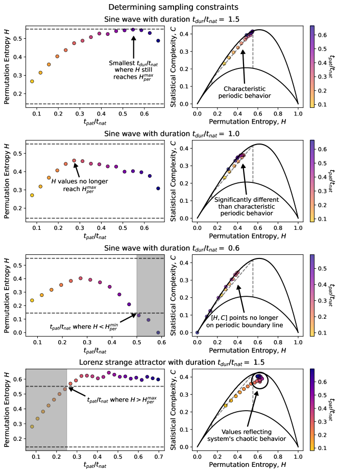
Figure 5: Illustration of method diagnostic for identifying sampling scheme constraints. Top row: $H(t_{\rm pat}/t_{\rm nat})$ and $HC$-plane plots for a sine wave time-series with a duration of $t_{\rm dur}/t_{\rm nat}=1.5$, with $t_{\rm nat}$ being the period of the sinusoid. The $HC$-plane on the right demonstrates the characteristic behavior of a periodic function, and the $H$-curve plot on the left shows that $H(t_{\rm pat}/t_{\rm nat})$, or $H(\ell)$ does not reach the $H_{\rm per}^{\rm max}$ upper limit. Second row: $H(t_{\rm pat}/t_{\rm nat})$ and $HC$-plane plots for a sine wave time-series with $t_{\rm dur}/t_{\rm nat}=1$, i.e., $t_{\rm dur}=t_{\rm nat}$. Both $H$-curve and $HC$-plane plots show that behavior deviates significantly from the characteristic behavior. Third row: $H(t_{\rm pat}/t_{\rm nat})$ and $HC$-plane plots for a sine wave time-series with $t_{\rm dur}/t_{\rm nat}=0.6$. $H$-curve shows the value for $t_{\rm pat}/t_{\rm nat}$ at which $H<H_{\rm per}^{\rm min}$. Points on $HC$-plane do not fall on the periodic boundary line. Fourth row: $H(t_{\rm pat}/t_{\rm nat})$ and $HC$-plane plots for a chaotic Lorenz strange attractor time-series with $t_{\rm dur}/t_{\rm nat}=1.5$. $H$-curve shows the location at which $H(t_{\rm pat}/t_{\rm nat})>H_{\rm per}^{\rm max}$, indicating the region where the chaotic time-series is reliably classified as complex. A circle on the $HC$-plane marks the accurately-classified points.

3.3 Interpreting PECCARY Values

There are two methods by which one can interpret the Permutation Entropy and Statistical Complexity values produced by PECCARY. The most exact way is to plot the $H$- and $C$-curves for each orbit within the system, though this can be difficult with many particles. This will show the different behaviors of the orbit(s) on different timescale probes, as regular, complex, and stochastic time-series all have different $H(\ell)$ and $C(\ell)$ shapes. Should the system be evolving with time, the timescale of the orbital behavior in question should be used to approximate the duration of the time-series, $t_{\rm dur}$, when considering the whether or not its nature can be discerned using a single orbit with PECCARY. As mentioned in Section 5, stacking techniques will be developed in a future publication.

For stochastic time-series, the Permutation Entropy and Statistical Complexity curves are close to constant, with $H(\ell)\sim 1$ and $C(\ell)\sim 0$. This is due to the fact that generated noise or stochasticity do not have any characteristic timescales.

Chaotic systems, on the other hand, have a characteristic shape to their curves that depend on whether they are discrete or continuous in nature. Discrete chaotic systems have a characteristic timescale that is inherently set to be $\ell=1$. As such, the maximum value for the Statistical Complexity occurs when $\ell=1$. By contrast, the maximum Statistical Complexity for continuous chaotic system depends on the approximate natural timescale. In terms of $H$- and $C$-curves, the value for Permutation Entropy increases with increasing sampling interval, while the value for Statistical Complexity increases to some maximum value at a particular pattern timescale, and then decreases. Examples of both discrete and chaotic maps are given in Sections 4.1.3 and 4.2.

Compared to stochastic and complex signals, regular time-series generally have smaller values for $H(\ell{=}1)$ that rise with increasing sampling interval. The $H$-curves of purely periodic time-series (such as a sine wave) also exhibit a characteristic pattern of $H(\ell)\rightarrow H_{\rm per}^{\rm max}$ at $t_{\rm pat}/t_{\rm nat}{\sim}0.6$ ratio and regularly returning to that value as the sampling interval continues to increase. This behavior is reflected in the $C$-curve as well (since $C$ depends on $H$), which results in a pure periodic function falling on or within the periodic boundary of the $HC$-plane for all sampling interval values. This is further discussed in Section 4.1.1.

However for very large datasets and many particles, generating $H$- and $C$-curves for each time-series can be impractical. The next-best method is to choose a sampling interval within the limits for $t_{\rm pat}/t_{\rm nat}$, as described in Section 3.2. The location of where the values fall within the $HC$-plane in Figure 4 result in the classification of the orbit type.

In the case of ambiguous cases, it may be necessary to incorporate additional methods, such as Fourier analysis in order to break some of the degeneracy/uncertainty. This will be the subject of a future paper in this series. See Section 5 for further discussion.

4 Examples

This section provides a variety of examples demonstrating the performance of the PECCARY method in systems with known outcomes. In Section 4.1, PECCARY is applied to several well-characterized, mathematical functions, while Section 4.3 demonstrates the usage of PECCARY on tracer particle simulations of four well-known orbital systems.

4.1 Well-Characterized Mathematical Examples

4.1.1 Sine wave

The sine wave is a classic example of a pure periodic function. This example generates five sine waves of different periods. Each of these time-series have a duration of $t_{\rm dur}=10~{}\mathrm{s}$, sampled at a resolution of $\delta t=2^{-8}~{}\mathrm{s}$, and the duration of each time-series is greater than at least five completed cycles ($t_{\rm dur}/t_{\rm nat}>5$).

Figure 6 shows how the values for the Permutation Entropy (top, left panel) and Statistical Complexity (top, middle panel) depend on the choice of sampling interval ($\ell$). The patterns in these plots are clearer when plotting both as a function of the pattern timescale divided by the period (i.e., natural timescale), $t_{\rm pat}/t_{\rm nat}$ (bottom panels). These panels illustrate that there is a characteristic shape to the Permutation Entropy and Statistical Complexity curves that depends on the period of the oscillatory behavior. The curve for the Permutation Entropy has a maximum value set by $H^{\rm max}_{\rm periodic}$ (Equation 7) with the exception of three spikes that are numerical artifacts. The $HC$-plane (top, right panel) shows the distributions for all choices for $\ell$.

Figure 6: Permutation Entropy and Statistical Complexity values for a range of sampling intervals for five sine waves of different periods. Top left panel: Permutation Entropy values for sampling intervals ranging from 1 to 200, with the corresponding pattern timescales on the top x-axis. Sine waves with smaller periods reach the $H_{\rm per}^{\rm max}(n=5)$ limit more quickly. Horizontal dashed lines in the two left panels represent the upper and lower limits of $H_{\rm per}^{\rm min}(n=5)$ and $H_{\rm per}^{\rm max}(n=5)$, respectively. Bottom left panel: The same Permutation Entropy values except that the x-axis is the pattern timescale scaled by the period of each sine wave (i.e., $t_{\rm pat}/t_{\rm nat}$). All five of the H-curves overlap exactly, with the exception of the numerical spikes. Top center panel: Statistical Complexity values as a function of sampling interval/pattern timescale. As with the H-curves, the sine waves with shorter periods reach the initial peak much more rapidly than those with longer periods. Bottom center panel: Statistical Complexity values plotted against the $t_{\rm pat}/t_{\rm nat}$ ratio show that the C-curves for the different sine waves have the same functional form. Top right panel: The $H$ and $C$ values for the five sine waves with ideal sampling ($t_{\rm pat}/t_{\rm nat}=0.4$, $t_{\rm dur}/t_{\rm nat}\geq 1$) plotted on the $HC$-plane all fall on or within the boundary region for a pure periodic function.

4.1.2 Noise varieties

PECCARY is effective for a variety of colors (or power spectra) of noise. Figure 7 shows the values for the Permutation Entropy (left panel) and Statistical Complexity (middle panel) as a function of the sampling interval ($\ell$) for five varieties of noise. These are white noise (power spectral density equal at all frequencies $\nu$), blue noise (power spectral density $\propto\nu$), violet noise (power spectral density $\propto\nu^{2}$), Brownian noise (also called red noise, power spectral density $\propto\nu^{-2}$), and pink noise (power spectral density $\propto\nu^{-1}$). Using PECCARY’s examples.noiseColors class, five sample time-series of $10^{4}$ discrete measures were created for the aforementioned noise colors.

Each noise spectrum has values on the $HC$-plane that are indicative of stochasticity. Furthermore, the Permutation Entropy and Statistical Complexity curves (i.e. $H(\ell)$ and $C(\ell)$) from any type of noise have nearly constant values for all choices for sampling interval $\ell$, where the value for $C$ is close to or near 0 and the value for $H$ is close to or near 1 at all scales. This is due to the fact that the value of the time-series at each time-step comes from a random distribution, which means the occurrence frequency of patterns at every sampling interval will always be at or very near uniform.

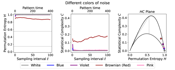
Figure 7: Permutation Entropy and Statistical Complexity values for a range of sampling intervals for five different colors of noise (pink, red, violet, blue, and white). Left panel: Permutation Entropy as a function of sampling interval/pattern timescale. All $H$ values are very high (close to $H=1$), indicating the presence of close to all possible permutations of patterns. Horizontal dashed lines represent the upper and lower limits of $H_{\rm per}^{\rm min}(n=5)$ and $H_{\rm per}^{\rm max}(n=5)$, respectively. Center panel: Statistical Complexity as a function of sampling interval/pattern timescale. $C$ values are very low for all colors of noise, indicating that the pattern probability distributions are close to uniform. Right panel: The $[H,C]$ values for sampling interval of $\ell=1$ plotted on the $HC$-plane for all noise varieties fall well within the stochastic region.

4.1.3 Chaotic systems

Two well-studied examples of chaos are the Hénon map (Eq. 11) and the Lorenz strange attractor. The Hénon map is a discrete chaotic map, while the Lorenz strange attractor is continuous. The Lorenz strange attractor is a system described by (Lorenz, 1963),

$$\frac{dx}{dt} =\sigma(y-x)$$ (12)

$$\frac{dy}{dt} =x(\rho-z)-y$$ (13)

$$\frac{dz}{dt} =xy-\beta z$$ (14)

which produces chaotic time-series. Figure 8 shows a 3D plot of the system using the standard parameters of $\sigma=10$, $\rho=20$, and $\beta=\frac{8}{3}$, which Lorenz used in his 1963 paper.

Four time-series are generated to diagnose PECCARY’s effectiveness for well-characterized chaotic systems: one from the Hénon map and three for the Cartesian coordinates of the Lorenz strange attractor.

While the idealized sampling scheme described in Section 3.2 uses the natural oscillatory timescale of a time-series, it can be difficult to identify a baseline oscillatory period for a chaotic time-series. This set of chaotic examples demonstrate two ways to approximate a relevant $t_{\rm nat}$ timescale.

If the timescale to probe is unknown, a rough oscillatory timescale can be determined by identifying the locations (in time) of the local maxima (or local minima) of the time-series, calculating the elapsed time between each peak, and taking the average of those values. This is called the “approximated $t_{\rm nat}$” method.

Alternately, the timescale at which the maximum Statistical Complexity ($C$) occurs can be used for the ideal sampling. In this method, the sampling interval corresponding to the peak value in the $C(\ell)$ curve is determined. From that value, the pattern timescale $t_{\rm pat}$ can be calculated (via Equation 1). Depending on the $t_{\rm pat}/t_{\rm nat}$ ratio used (typically 0.4), that $t_{\rm pat}$ value can be used to find the natural oscillatory timescale $t_{\rm nat}$. This is called the “$t_{\rm nat}$ from maximum $C(\ell)$” method.

Figure 9 illustrates the difference in how discrete and continuous chaotic maps behave in $H(\ell)$ and $C(\ell)$ curves when applying PECCARY to the four different time-series. While both types of chaotic maps increase in Permutation Entropy $H$ as the sampling interval $\ell$ increases, in Statistical Complexity, the discrete map falls from its initial value and stays constant, while the continuous map increases and then eventually drops as the sampling interval increases. The $HC$-plane shows the $[H,C]$ values calculated from ideal sampling with the “approximated $t_{\rm nat}$ method” as circles and those calculated with the “$t_{\rm nat}$ from maximum $C(\ell)$” method as diamonds. All points fall within the chaotic regime of the $HC$-plane.

This exercise illustrates that a chaotic time-series may appear to be entirely stochastic if it is sampled at sampling intervals where favored or forbidden patterns cannot be resolved. A chaotic signal may have multiple characteristic timescales for favored and forbidden patterns, but these can only be discerned within the timescales explored by the selected range of sampling interval. In addition, the optimal sampling size, $n$, can be modified in consideration of sampling favored patterns for more or less complex or lengthy patterns.

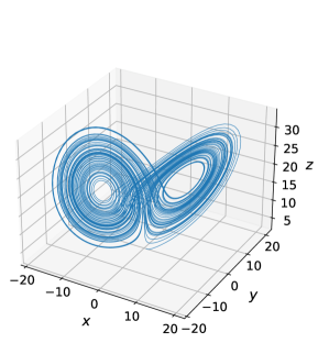
Figure 8: Three dimensional plot of the Lorenz strange attractor with parameters $\sigma=10$, $\rho=20$, and $\beta=2.667$.

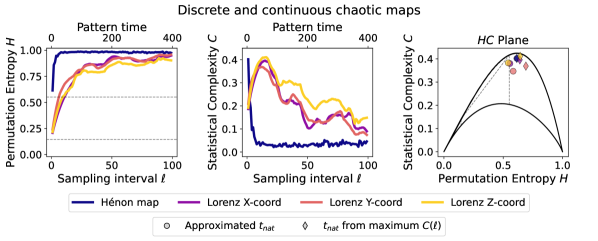
Figure 9: Permutation Entropy and Statistical Complexity values for a range of sampling intervals for the discrete Hénon map and the continuous x/y/z-coordinates of the Lorenz strange attractor. Left panel: Permutation Entropy as a function of sampling interval/pattern timescale. For all time-series, the $H$ values increase initially and approach 1 rapidly (for a discrete chaotic system) or gradually (for a continuous chaotic system). Horizontal dashed lines represent the upper and lower limits of $H_{\rm per}^{\rm min}(n=5)$ and $H_{\rm per}^{\rm max}(n=5)$, respectively. Center panel: Statistical Complexity as a function of sampling interval/pattern timescale. For the discrete chaotic map, the $C$ values drop rapidly and bottom out close to zero. With the continuous chaotic map, the values of $C$ initially increase and then gradually decrease. Right panel: The $[H,C]$ values plotted on the $HC$-plane for the different chaotic systems span across the $HC$-plane at ideal sampling. $[H,C]$ points calculated using the “approximated $t_{\rm nat}$” method are shown as circles, while those determined with the “$t_{\rm nat}$ from maximum $C(\ell)$” method are represented as diamonds. All values fall within the chaotic regime.

4.2 Double Pendulum

PECCARY’s examples.doublePendulum was used to generate time-series for a double pendulum system. The model assumes upper and lower pendulum masses of 1 kg each and pendulum lengths of 1 m. The system was allowed to evolve for a range of times (i.e., 2.5 s, 5 s, 10 s, 50 s, and 100 s) at a time resolution (i.e., step size) of $\delta t=2^{-6}$ s. Figure 10 shows that while certain durations (e.g., 5 s and 10 s) remain in the complex region after turning off from the periodic/regular regime, too short of a duration (e.g., 2.5 s) will appear regular. The sampling for the longer durations (50 s and 100 s) show that too large of a sampling interval will cause chaotic behavior to appear as noise on the $HC$-plane. With the idealized sampling scheme, all the $[H,C]$ points fall in the complex regime, with the exception of the too-short 2.5 s simulation.

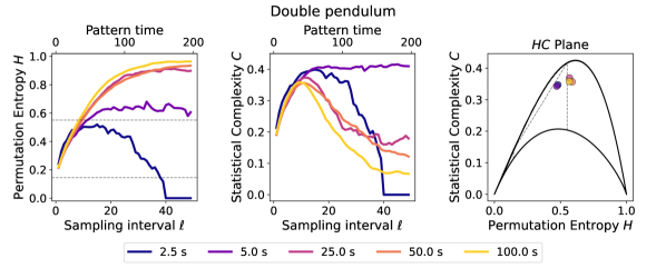
Figure 10: Permutation Entropy and Statistical Complexity values for a range of sampling intervals for the double pendulum. Left panel: Permutation Entropy as a function of sampling interval/pattern timescale. For all time-series, the $H$ values increase gradually. Horizontal dashed lines represent the upper and lower limits of $H_{\rm per}^{\rm min}(n=5)$ and $H_{\rm per}^{\rm max}(n=5)$, respectively. Center panel: Statistical Complexity as a function of sampling interval/pattern timescale. For all simulation  durations, the values of $C$ initially increase and then gradually decrease, with the exception of the shortest simulations. Right panel: The $[H,C]$ values plotted on the $HC$-plane for the different simulation durations at ideal sampling. All values fall within the complex regime, with the exception of the 2.5 s simulation.

4.3 Astrophysical Examples

The tracer particle simulations for the astrophysical examples in the following subsections were created with galpy (Bovy, 2015), using the symplec4_c integrator.

4.3.1 Keplerian Potential

While there are many types of regular orbits in astrophysics, only the point-mass (i.e., Keplerian) potential produces a special case of non-circular orbits that close in a single period, due to the fact that the radial and azimuthal frequencies are equal. As such, the Keplerian potential is an ideal scenario for testing regular orbits that close after $2\pi$. In this case, galpy’s Orbit.from_name(’solar system’) function was used to create a tracer-particle simulation of the orbits of the eight planets of the solar system for a duration of 100 years, at a resolution of 2.85 days. Figure 11 demonstrates that all the values fall on and within the periodic/regular boundary of the $HC$-plane when using the x-coordinate for the orbits.

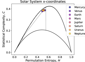
Figure 11: $HC$-plane showing the $[H,C]$ coordinates for tracer particle simulation x-coordinates of the Solar System when $t_{\rm pat}/t_{\rm nat}=0.4$. All data points fall within the periodic/regular boundary, consistent with the fact that these are circular orbits.

4.3.2 Globular Cluster

A spherical potential is a minimally intricate astrophysical example for testing the PECCARY method. Using a spherical Plummer potential (galpy.potential.PlummerPotential) and self-consistent isotropic and spherical Plummer distribution function (galpy.df.isotropicPlummerdf), $10^{4}$ tracer particles (representing stars) were evolved for a duration of 1 Gyr and an orbit integration time resolution of 0.1 Myr. Figure 12 shows a sampling of 50 stellar orbits plotted on the $HC$-plane based on the $[H,C]$ values calculated from the x-coordinates of orbits with $t_{\rm dur}/t_{\rm pat}\geq 1.5$ and $t_{\rm pat}/t_{\rm nat}=0.4$. Many orbits fall on or within the periodic/regular boundary, with others falling within the “regular” regime. The divergence from the periodic boundary line is likely due to the fact that these are not closed orbits. The PECCARY method will be developed further for investigating regimes such as this in a future paper.

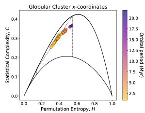
Figure 12: $HC$-plane showing the $[H,C]$ values when $t_{\rm pat}/t_{\rm nat}=0.4$ for globular cluster tracer particles. The x-coordinates are used for the PECCARY method, with orbital periods satisfying the $t_{\rm dur}/t_{\rm nat}\geq 1.5$ requirement. Most of the $[H,C]$ values fall on or within the periodic/regular boundary/region, though some have lower complexity values. None of the $[H,C]$ values for the orbits exceed the $H_{\rm per}^{\rm max}$ limit for $n=5$, consistent with the expectation that all of the orbits for a spherical potential are regular.

4.3.3 Triaxial Halo

A triaxial potential will exhibit regular orbits, as well as chaotic orbits. To verify that PECCARY returns this same conclusion, a tracer-particle simulation of a Navarro-Frenk-White (NFW) potential (galpy.potential.TriaxialNFWPotential) was created with an isotropic NFW distribution function that samples a spherical NFW halo (galpy.df.isotropicNFWdf). The default galpy settings were used for the triaxial prescription, with the exception of the y/x and z/x axis ratios. These two ratios are referred to as $b$ and $c$, respectively, and were set to $b=1.66$ and $c=3$ with a normalization of 0.35 based on the reported values for a Milky Way-like halo in Rojas-Niño et al. (2012); Hesp & Helmi (2018). $10^{4}$ stars were evolved for a duration of 100 Gyr at a time resolution of 15.625 Myr.

Figure 13 shows $[H,C]$ values at $t_{\rm pat}/t_{\rm nat}=0.4$ for the x-coordinates of simulated stars with $t_{\rm dur}/t_{\rm nat}\geq 1.5$. Several of the orbits fall within the regular regime, where many of these were visually identified as tube orbits. Some orbits, particularly those with shorter orbital periods, have time-series characteristics that are highly complex. Future work will compare the results from PECCARY to other known diagnostics of chaos.

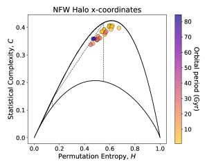
Figure 13: $HC$-plane showing the $[H,C]$ values when $t_{\rm pat}/t_{\rm nat}=0.4$ for triaxial NFW halo tracer particles. The x-coordinates are used for the PECCARY method, with orbital periods satisfying the $t_{\rm dur}/t_{\rm nat}\geq 1.5$ requirement. As expected for a triaxial potential, there is a mix particles falling in both the regular and complex zones.

4.3.4 Injected Noise

To test the sensitivity of PECCARY on several idealized examples of “noisy data,” different levels of noise were injected to the various orbits presented in Section 4.3.1-4.3.3. The noise injections were determined by calculating the approximate amplitude of each orbital x-coordinate time-series (i.e., maximum absolute value less the average value) and then adding a random value to each time-step. The random “errors” were drawn from a uniform distribution ranging from -1 to 1 and were then scaled by the amplitude of the time-series and the fraction of the noise (i.e., 0.1, 0.5, or 1). The noise injection “percentages” are defined as the amplitude of the noise relative to the amplitude of the signal.

Figure 14 compares values on the $HC$-planes of the three noise levels at sampling intervals equivalent to $t_{\rm pat}/t_{\rm nat}=0.4$ and for orbits with $t_{\rm dur}/t_{\rm nat}\geq 1.5$. Compared to the original datasets, periodic and regular orbits with injected noise appear to increase primarily in $H$, while complex orbits appear to have similar $[H,C]$ coordinates. To the level of 10% noise, the $[H,C]$ values have shifted significantly compared to the pure signals, although they do not appear as stochastic. At 50% and 100% noise, almost all or all of the $[H,C]$ points fall primarily within the stochastic region.

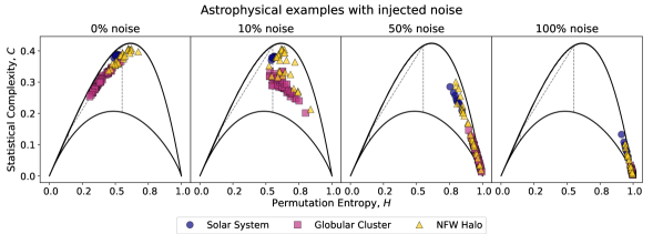
Figure 14: $HC$-planes showing the effect of noise injection on the PECCARY method for the three astrophysical example potentials. Circle, square, and triangle markers represent the Solar System, globular cluster, and triaxial halo simulations respectively. Left panel: Original $[H,C]$ values, as shown in Figures 11-13. Left-center panel: $[H,C]$ values for the three potentials with noise amplitude at 10% of the signal amplitude. Regular orbits appear to fall either within the regular region or below the primary complex region. Complex orbits still fall within the region of maximum complexity. Right-center panel: $[H,C]$ values for the three potentials with noise amplitude at 50% of the signal amplitude. Almost all of the values appear to fall within the stochastic region. Right panel: $[H,C]$ values for the three potentials with noise amplitude equal to the signal amplitude. All of the values to fall within the stochastic region.

5 Future Work

This paper introduces the PECCARY method for usage in astrophysics. While the measures of Permutation Entropy and Statistical Complexity have been used in other fields, including plasma physics (Weck et al., 2015), to great success, those bodies of work involved systems or models that were inherently discrete and could use a sampling interval of $\ell=1$. The fundamentally continuous nature of many astrophysical systems, as well as the varied origin of stochasticity (i.e., natural noise or background sources/behaviors), require great care with choosing the appropriate sampling schemes. The PECCARY method provides the first clear recommendations for using Permutation Entropy and Statistical Complexity measures to characterize the behaviors of continuous systems.

This study investigates how well the method works for several astrophysical systems with known behaviors (Section 4.3), but additional work is needed for widespread uses. Future papers will develop a method for estimating the confidence of the periodic/regular/chaotic/stochastic diagnosis and run comparisons with existing methods for chaos identification, such as frequency analysis mapping (Laskar, 1990; Valluri & Merritt, 1998; Valluri et al., 2012, 2016; Beraldo e Silva et al., 2019, 2023) and potentially Lyapanov exponents to test the robustness of PECCARY in this regime.

While Section 4.3.4 demonstrated an example of PECCARY’s ability to handle noise injected into a known system, additional work is needed on understanding the sensitivities of the method for characterizing orbital behavior in a noisy signal. Future research will center on developing more intricate astrophysical simulations (e.g., evolving, time-dependent potentials and large-scale n-body simulations) to test the PECCARY method. Other work will explore the efficacy of stacking time-series in order to improve reliability for shorter duration simulations and windowing, for understanding how a system changes dynamically over time.

6 Conclusions

This paper introduces the PECCARY method to the astrophysics community for the first time. PECCARY is a statistical method that samples ordinal patterns from any sort of time-series, creates a probability distribution of all possible permutations of those patterns, and calculates the Permutation Entropy $H$ and Statistical Complexity $C$ from that distribution. The location that these Permutation Entropy and Statistical Complexity coordinate values fall on the $HC$-plane indicate the classification of the orbital behavior.

This paper provides an overview of the underlying theory and discuss best practices for initial implementations of the PECCARY method. This work also demonstrates that for pure periodic functions, the orbital period can be easily extracted by using the shapes and initial peak of the $H(\ell)$ curves.

The PECCARY method is effective for time-series where the overall duration of the time-series is at minimum equal to the approximate period of the orbit, though a ration of $t_{\rm dur}/t_{\rm nat}\gtrsim 1.5$ is ideal. While the overall shapes of the $H(\ell)$ and $C(\ell)$ curves provide the best indication for classifying the behavior of the data, in many cases it is better to necessary or more efficient to sample a single method. For cases such as these, the ratio between the pattern timescale and the period should be between 0.3 and 0.5, i.e., $0.3\lesssim t_{\rm pat}/t_{\rm nat}\lesssim 0.5$. The corresponding sampling interval can be calculated with the PECCARY package or using Equation 1.

Finally, a variety of different examples, both mathematical and astrophysical, are presented as a proof of concept of PECCARY. Additional tests of the method’s sensitivity, limitations, and wider applications will be presented in future papers in this series.

Extensive documentation and examples for the corresponding PECCARY Python package are available online. The source code can be found on GitHub and builds can be found on the PyPI project page.

References

- Araujo et al. (2020) Araujo, F. H. A. d., Bejan, L., Stosic, B., & Stosic, T. 2020, Chaos, Solitons Fractals, 139, 110081, doi: https://doi.org/10.1016/j.chaos.2020.110081
- Aronis et al. (2018) Aronis, K. N., Berger, R. D., Calkins, H., et al. 2018, Chaos, 28, 063130, doi: 10.1063/1.5023588
- Astakhov et al. (2003) Astakhov, S. A., Burbanks, A. D., Wiggins, S., & Farrelly, D. 2003, Nature, 423, 264, doi: 10.1038/nature01622
- Athanassoula et al. (1983) Athanassoula, E., Bienayme, O., Martinet, L., & Pfenniger, D. 1983, A&A, 127, 349
- Bandt & Pompe (2002) Bandt, C., & Pompe, B. 2002, Phys. Rev. Lett., 88, 174102, doi: 10.1103/PhysRevLett.88.174102
- Bariviera et al. (2013) Bariviera, A. F., Zunino, L., Guercio, M. B., Martinez, L. B., & Rosso, O. A. 2013, J. Stat. Mech. Theory Exp., 2013, P08007. http://stacks.iop.org/1742-5468/2013/i=08/a=P08007
- Beraldo e Silva et al. (2019) Beraldo e Silva, L., de Siqueira Pedra, W., Valluri, M., Sodré, L., & Bru, J.-B. 2019, ApJ, 870, 128, doi: 10.3847/1538-4357/aaf397
- Beraldo e Silva et al. (2023) Beraldo e Silva, L., Debattista, V. P., Anderson, S. R., et al. 2023, ApJ, 955, 38, doi: 10.3847/1538-4357/ace976
- Bovy (2015) Bovy, J. 2015, ApJS, 216, 29, doi: 10.1088/0067-0049/216/2/29
- Calbet & Lopez-Ruiz (2001) Calbet, & Lopez-Ruiz, R. 2001, Physical review. E, Statistical, nonlinear, and soft matter physics, 63, 066116
- Cao et al. (2004) Cao, Y., Tung, W.-w., Gao, J. B., Protopopescu, V. A., & Hively, L. M. 2004, Phys. Rev. E, 70, 046217. https://link.aps.org/doi/10.1103/PhysRevE.70.046217
- Contopoulos (1990) Contopoulos, G. 1990, Proceedings of the Royal Society of London Series A, 431, 183, doi: 10.1098/rspa.1990.0126
- Deck et al. (2013) Deck, K. M., Payne, M., & Holman, M. J. 2013, ApJ, 774, 129, doi: 10.1088/0004-637X/774/2/129
- Dehnen (2001) Dehnen, W. 2001, MNRAS, 324, 273, doi: 10.1046/j.1365-8711.2001.04237.x
- Donner et al. (2015) Donner, R. V., Potirakis, S. M., Balasis, G., Eftaxias, K., & Kurths, J. 2015, Physics and Chemistry of the Earth, Parts A/B/C, 85-86, 44. http://www.sciencedirect.com/science/article/pii/S1474706515000327
- Fernandes et al. (2020) Fernandes, L. H., de Araújo, F. H., & Silva, M. A. 2020, Research Square, doi: 10.21203/rs.3.rs-36581/v1+
- Fux (2001) Fux, R. 2001, A&A, 373, 511, doi: 10.1051/0004-6361:20010561
- Gekelman et al. (2014) Gekelman, W., Compernolle, B. V., DeHaas, T., & Vincena, S. 2014, Plasma Physics and Controlled Fusion, 56, 064002. http://stacks.iop.org/0741-3335/56/i=6/a=064002
- Gekelman et al. (2014) Gekelman, W., Van Compernolle, B., DeHaas, T., & Vincena, S. 2014, Plasma Physics and Controlled Fusion, 56, 064002
- Gladman (1993) Gladman, B. 1993, Icarus, 106, 247, doi: 10.1006/icar.1993.1169
- Good et al. (2020) Good, S. W., Ala-Lahti, M., Palmerio, E., Kilpua, E. K. J., & Osmane, A. 2020, ApJ, 893, 110, doi: 10.3847/1538-4357/ab7fa2
- Hénon (1976) Hénon, M. 1976, Communications in Mathematical Physics, 50, 69, doi: 10.1007/BF01608556
- Hesp & Helmi (2018) Hesp, C., & Helmi, A. 2018, arXiv e-prints, arXiv:1804.03670, doi: 10.48550/arXiv.1804.03670
- Jordan et al. (2008) Jordan, D., Stockmanns, G., Kochs, E. F., Pilge, S., & Schneider, G. 2008, Anesthesiology, 109, 1014, doi: 10.1097/ALN.0b013e31818d6c55
- Kandrup & Willmes (1994) Kandrup, H. E., & Willmes, D. E. 1994, A&A, 283, 59
- Lamberti et al. (2004) Lamberti, P. W., Martin, M. T., Plastino, A., & Rosso, O. A. 2004, Physica A: Statistical Mechanics and its Applications, 334, 119
- Laskar (1990) Laskar, J. 1990, Icarus, 88, 266, doi: 10.1016/0019-1035(90)90084-M
- Laskar et al. (1992) Laskar, J., Froeschlé, C., & Celletti, A. 1992, Physica D Nonlinear Phenomena, 56, 253, doi: 10.1016/0167-2789(92)90028-L
- Li et al. (2010) Li, D., Li, X., Liang, Z., Voss, L. J., & Sleigh, J. W. 2010, Journal of Neural Engineering, 7, 046010. http://stacks.iop.org/1741-2552/7/i=4/a=046010
- Lithwick & Wu (2011) Lithwick, Y., & Wu, Y. 2011, ApJ, 739, 31, doi: 10.1088/0004-637X/739/1/31
- López-Ruiz et al. (1995) López-Ruiz, R., Mancini, H. L., & Calbet, X. 1995, Physics Letters A, 209, 321
- Lorenz (1963) Lorenz, E. N. 1963, Journal of the Atmospheric Sciences, 20, 130, doi: 10.1175/1520-0469(1963)020<0130:DNF>2.0.CO;2
- Maggs & Morales (2013) Maggs, J. E., & Morales, G. J. 2013, Plasma Physics and Controlled Fusion, 55, 085015. http://stacks.iop.org/0741-3335/55/i=8/a=085015
- Maggs et al. (2015) Maggs, J. E., Rhodes, T. L., & Morales, G. J. 2015, Plasma Physics and Controlled Fusion, 57, 045004. http://stacks.iop.org/0741-3335/57/i=4/a=045004
- Malhotra (1993) Malhotra, R. 1993, Nature, 365, 819, doi: 10.1038/365819a0
- Manos & Athanassoula (2011) Manos, T., & Athanassoula, E. 2011, MNRAS, 415, 629, doi: 10.1111/j.1365-2966.2011.18734.x
- Martinet (1974) Martinet, L. 1974, A&A, 32, 329
- Merritt & Poon (2004) Merritt, D., & Poon, M. Y. 2004, ApJ, 606, 788, doi: 10.1086/382497
- Murray-Clay & Chiang (2006) Murray-Clay, R. A., & Chiang, E. I. 2006, ApJ, 651, 1194, doi: 10.1086/507514
- Neyrinck et al. (2022) Neyrinck, M., Genel, S., & Stücker, J. 2022, arXiv e-prints, arXiv:2206.10666, doi: 10.48550/arXiv.2206.10666
- Olivier et al. (2019) Olivier, C. P., Engelbrecht, N. E., & Strauss, R. D. 2019, Journal of Geophysical Research: Space Physics, 124, 4, doi: 10.1029/2018JA026102
- Papaphilippou & Laskar (1996) Papaphilippou, Y., & Laskar, J. 1996, A&A, 307, 427
- Papaphilippou & Laskar (1998) —. 1998, A&A, 329, 451
- Patsis (2006) Patsis, P. A. 2006, MNRAS, 369, L56, doi: 10.1111/j.1745-3933.2006.00174.x
- Pfenniger (1986) Pfenniger, D. 1986, A&A, 165, 74
- Pichardo et al. (2003) Pichardo, B., Martos, M., Moreno, E., & Espresate, J. 2003, ApJ, 582, 230, doi: 10.1086/344592
- Poincaré (1891) Poincaré, H. 1891, Bulletin Astronomique, Serie I, 8, 12
- Price-Whelan et al. (2016) Price-Whelan, A. M., Johnston, K. V., Valluri, M., et al. 2016, MNRAS, 455, 1079, doi: 10.1093/mnras/stv2383
- Ribeiro et al. (2017) Ribeiro, H. V., Jauregui, M., Zunino, L., & Lenzi, E. K. 2017, Phys. Rev. E, 95, 062106. https://link.aps.org/doi/10.1103/PhysRevE.95.062106
- Rojas-Niño et al. (2012) Rojas-Niño, A., Valenzuela, O., Pichardo, B., & Aguilar, L. A. 2012, ApJ, 757, L28, doi: 10.1088/2041-8205/757/2/L28
- Rosso et al. (2007) Rosso, O. A., Larrondo, H. A., Martin, M. T., Plastino, A., & Fuentes, M. A. 2007, Phys. Rev. Lett., 99, 154102, doi: 10.1103/PhysRevLett.99.154102
- Saha & Tremaine (1993) Saha, P., & Tremaine, S. 1993, Icarus, 106, 549, doi: 10.1006/icar.1993.1192
- Schaap & van de Weygaert (2000) Schaap, W. E., & van de Weygaert, R. 2000, A&A, 363, L29. https://arxiv.org/abs/astro-ph/0011007
- Schuster (1988) Schuster, H. G. 1988, Deterministic chaos: An introduction (2nd revised edition) (Weinheim)
- Sellwood (2014) Sellwood, J. A. 2014, Reviews of Modern Physics, 86, 1, doi: 10.1103/RevModPhys.86.1
- Sellwood & Debattista (2009) Sellwood, J. A., & Debattista, V. P. 2009, MNRAS, 398, 1279, doi: 10.1111/j.1365-2966.2009.15219.x
- Serinaldi et al. (2014) Serinaldi, F., Zunino, L., & Rosso, O. A. 2014, Stochastic Environmental Research and Risk Assessment, 28, 1685, doi: 10.1007/s00477-013-0825-8
- Shannon (1948) Shannon, C. E. 1948, The Bell System Technical Journal, 27, 379
- Suyal et al. (2012) Suyal, V., Prasad, A., & Singh, H. P. 2012, Solar Physics, 276, 407, doi: 10.1007/s11207-011-9889-0
- Suzuki & Maeda (2000) Suzuki, S., & Maeda, K.-I. 2000, Phys. Rev. D, 61, 024005, doi: 10.1103/PhysRevD.61.024005
- Thaxton et al. (2018) Thaxton, C. S., Anderson, W. P., Gu, C., Stosic, B., & Stosic, T. 2018, Stochastic Environmental Research and Risk Assessment, 32, 843, doi: 10.1007/s00477-017-1434-8
- Valluri et al. (2012) Valluri, M., Debattista, V. P., Quinn, T. R., Roškar, R., & Wadsley, J. 2012, MNRAS, 419, 1951, doi: 10.1111/j.1365-2966.2011.19853.x
- Valluri & Merritt (1998) Valluri, M., & Merritt, D. 1998, ApJ, 506, 686, doi: 10.1086/306269
- Valluri et al. (2016) Valluri, M., Shen, J., Abbott, C., & Debattista, V. P. 2016, ApJ, 818, 141, doi: 10.3847/0004-637X/818/2/141
- Varadi et al. (2003) Varadi, F., Runnegar, B., & Ghil, M. 2003, ApJ, 592, 620, doi: 10.1086/375560
- Weck et al. (2015) Weck, P. J., Schaffner, D. A., Brown, M. R., & Wicks, R. T. 2015, Phys. Rev. E, 91, 023101. https://link.aps.org/doi/10.1103/PhysRevE.91.023101
- Weinberg (2015a) Weinberg, M. D. 2015a, arXiv e-prints, arXiv:1508.06855. https://arxiv.org/abs/1508.06855
- Weinberg (2015b) —. 2015b, arXiv e-prints, arXiv:1508.05959. https://arxiv.org/abs/1508.05959
- Weygand & Kivelson (2019) Weygand, J. M., & Kivelson, M. G. 2019, ApJ, 872, 59, doi: 10.3847/1538-4357/aafda4
- Zhu et al. (2017) Zhu, Z., White, A. E., Carter, T. A., Baek, S. G., & Terry, J. L. 2017, Physics of Plasmas, 24, 042301, doi: 10.1063/1.4978784
- Zunino et al. (2012) Zunino, L., Soriano, M. C., & Rosso, O. A. 2012, Physical Review E, 86, 046210
- Zunino et al. (2010) Zunino, L., Zanin, M., Tabak, B. M., Perez, D. G., & Rosso, O. A. 2010, Physica A: Statistical Mechanics and its Applications, 389, 1891. http://www.sciencedirect.com/science/article/pii/S0378437110000397