mochi_class: Modelling Optimisation to Compute Horndeski in class

Abstract

We introduce mochi_class, an extension of the Einstein-Boltzmann solver hi_class, designed to unlock the full phenomenological potential of Horndeski gravity. This extension allows for general input functions of time without the need for hard-coded parametrisations or covariant Lagrangians. By replacing the traditional $\alpha$-parametrisation with a set of stable basis functions, mochi_class ensures that the resulting effective theories are inherently free from gradient and ghost instabilities. Additionally, mochi_class features a quasi-static approximation implemented at the level of modified metric potentials, enhancing prediction accuracy, especially for models transitioning between a super- and sub-Compton regime. mochi_class can robustly handle a wide range of models without fine-tuning, and introduces a new approximation scheme that activates modifications to the standard cosmology deep in the matter-dominated era. Furthermore, it incorporates viability conditions on the equation of motion for the scalar field fluctuations, aiding in the identification of numerical instabilities. Through comprehensive validation against other Einstein-Boltzmann solvers, mochi_class demonstrates excellent performance and accuracy, broadening the scope of hi_class by facilitating the study of specific modified gravity models and enabling exploration of previously inaccessible regions of the Horndeski landscape. The code is publicly available at https://github.com/mcataneo/mochi_class_public.

1 Introduction

The current cosmological paradigm ($\Lambda$CDM) is capable of describing the dynamics of the universe, the Cosmic Microwave Background (CMB) and the Large-Scales Structure (LSS) of the universe with only six parameters (Aghanim et al., 2018). On top of standard model particles, it assumes two exotic components whose nature is unknown: (i) a cosmological constant ($\Lambda$) and some form of Cold Dark Matter (CDM). The gravitational interactions are regulated by General Relativity (GR). This modelling explains the observed accelerated expansion of the universe (Riess et al., 1998; Perlmutter et al., 1998), and it provides a good fit to the data (e.g., Heymans et al., 2020; eBOSS Collaboration et al., 2020; DES Collaboration et al., 2021; Miyatake et al., 2023).

However, the standard cosmological model is unsatisfactory as it suffers from at least three drawbacks: (i) the value of the observed cosmological constant is too small to be explained by fundamental physics (Martin, 2012), (ii) GR is tested very precisely on local scales (Will, 2014) but it is extrapolated over 15 orders of magnitude in length scale to be applied to cosmological data (Peebles, 2004), and (iii) comparing different datasets produces tensions for the measured parameters (Valentino et al., 2021; Abdalla et al., 2022). In particular, the most significant is the Hubble tension, arising when combining “early” and “late” times measurements of the expansion rate of the universe (Verde et al., 2019).

To alleviate these problems several possible extensions have been proposed, either promoting $\Lambda$ to a dynamical field (Dark Energy, DE) (see, e.g., Copeland et al., 2006, for a review) or modifying the laws of gravity at cosmological scales (MG) (see, e.g., Clifton et al., 2011; Joyce et al., 2014, 2016, for reviews). A unifying framework is realised by the Horndeski theory, that encompasses many of the scalar-tensor theories proposed in the literature, e.g. Quintessence, $f(R)$ gravity, Brans-Dicke, Galileons. Horndeski gravity provides one of the most general scalar-tensor theories with at most second-order derivatives in the equations of motion on any background (Horndeski, 1974; Deffayet et al., 2009a; Kobayashi et al., 2011). It gained significant popularity due to its rich phenomenology while remaining analytically tractable.

To study the Horndeski landscape, there are two potential strategies (e.g., Ezquiaga & Zumalacárregui, 2018). It is possible to: (i) select a specific model based on its covariant Lagrangian formulation and analyse the effects of the additional degree of freedom across different regimes, from cosmological scales to compact objects and black holes; or (ii) adopt an effective-theory approach (EFT), focusing solely on the energy scales relevant to cosmology.

While strategy (i) allows for a detailed investigation of particular scalar-tensor theories, it demands significant resources and time investment. In the absence of a compelling alternative to GR, strategy (ii) provides a more general and efficient method to detect or constrain deviations from standard gravity (e.g., Ezquiaga & Zumalacárregui, 2017; Creminelli & Vernizzi, 2017; Baker et al., 2017; Sakstein & Jain, 2017).

Given the large classes of models that the Horndeski Lagrangian encapsulates, there have been countless attempts to get cosmological constraints on specific parametrisations. Following each one of the two distinct approaches described above, in the literature it is possible to find both constraints based on sub-classes of Horndeski (see, e.g., Joudaki et al., 2022; Zumalacárregui, 2020; Ye & Silvestri, 2024), and on different parametrisations of the EFT functions (see, e.g., Bellini et al., 2015; Kreisch & Komatsu, 2017; Noller & Nicola, 2018; Mancini et al., 2019; Seraille et al., 2024; Castello et al., 2024; Chudaykin & Kunz, 2024). A promising but less explored direction is to get model independent constraints. The idea is to try to “reconstruct” gravity without imposing an a priori time dependence for the EFT functions (Zhao et al., 2009, 2010; Hojjati et al., 2012; Raveri, 2019; Pogosian et al., 2021; Raveri et al., 2021; Park et al., 2021).

The public version of hi_class (Zumalacarregui et al., 2016; Bellini et al., 2019), an extension of the Einstein-Botzmann solver class (Blas et al., 2011; Lesgourgues, 2011a), implements both approaches, allowing users to easily implement new models belonging to Horndeski scalar-tensor theories or the EFT framework with the basis proposed in Bellini & Sawicki (2014). In a second release of the code, Bellini et al. (2019) included the quasi-static approximation scheme for improved computational efficiency and to extend the code’s applicability to models where following the full dynamics of the scalar field can be extremely challenging.

Even with these significant advances, further steps are required to reliably extend hi_class across a broader range of the Horndeski landscape. First, we need to simplify the implementation of specific models and parametrisations, which currently requires modifications to the source code. Additionally, efficient selection of stable models is crucial to avoid extensive searches for parameter combinations free from ghost and gradient instabilities. The accuracy of the QSA implementation in hi_class can be improved. Furthermore, addressing numerical noise from limited precision in the calculation of the scalar field speed of sound is essential to prevent incorrectly labeling healthy models as unstable.

To address these issues, in this paper we introduce mochi_class, a numerical tool to facilitate the study and statistical analysis of Horndeski models expressed in the effective-theory language. To improve flexibility, mochi_class externalises the models definition, allowing to pass to the code precomputed arrays for the time evolution of the background and the EFT functions. In addition, it implements a new stable parametrisation, to satisfy the stability conditions by construction. Furthemore, we implement a new integrated approximation scheme to switch on gravity modifications only after a certain (user specified) redshift. This fixes the early time evolution to $\Lambda$CDM, avoiding numerical instabilities when deviations from standard gravity are irrelevant. Finally, mochi_class implements an additional QSA approximation implemented at the level of modified metric potentials in Newtonian gauge. This offers a cross-check with the standard hi_class implementation and improves the agreement with the exact solution.

Throughout the paper we assume the speed of light $c=1$ and use the following values for the cosmological parameters: for the fractional energy-density of the cold dark matter and baryons, we set $\Omega_{\rm c}h^{2}=0.120108$ and $\Omega_{\rm b}h^{2}=0.022383$; for the Hubble constant, $h=0.6781$; for the amplitude and slope of the primordial power spectrum, $10^{9}A_{\rm s}=2.10055$ and $n_{\rm s}=0.96605$; for the optical depth at reionisation, $\tau=0.054308$.

The paper is organised as follow. In Section 2 we introduce the Horndeski models and their EFT description. In Section 3 we describe the code structure and implementation, and in Section 4 we validate it against other codes. In Section 5 we present a new parametrisation, and leave Section 6 for the summary and outlook.

2 Horndeski’s theory and parametrisations

In our analysis we focus on sub-classes of the Horndeski theory, one of the most general scalar-tensor theories with at most second-order equations of motion on any background (Horndeski, 1974; Deffayet et al., 2009a; Kobayashi et al., 2011). Its action can be written as

$$S_{\rm H}[g_{\mu\nu},\phi]=\int\mathrm{d}^{4}x\,\sqrt{-g}\left[\sum_{i=2}^{5}\frac{1}{8\pi G_{\mathrm{N}}}{\cal L}_{i}[g_{\mu\nu},\phi]+\mathcal{L}_{m}\right]\,,$$ (1a)

$${\mathcal{L}}_{2}=G_{2}(\phi,\,X)\,,$$ (1b)

$${\mathcal{L}}_{3}=-G_{3}(\phi,\,X)\Box\phi\,,$$ (1c)

$${\mathcal{L}}_{4}=G_{4}(\phi,\,X)R+G_{4X}(\phi,\,X)\left[\left(\Box\phi\right)^{2}-\phi_{;\mu\nu}\phi^{;\mu\nu}\right]\,,$$ (1d)

$${\mathcal{L}}_{5}=G_{5}(\phi,\,X)G_{\mu\nu}\phi^{;\mu\nu}$$

$$\quad\quad-{\frac{1}{6}}G_{5X}(\phi,\,X)\left[(\Box\phi)^{3}+2\phi_{;\mu}{}^{\nu}\phi_{;\nu}{}^{\alpha}\phi_{;\alpha}{}^{\mu}\right.$$

$$\quad\quad\left.{}-3\phi_{;\mu\nu}\phi^{;\mu\nu}\Box\phi\right].$$ (1e)

Here, $g_{\mu\nu}$ is the metric tensor, $\mathcal{L}_{m}$ is the matter Lagrangian and $G_{2,\,3,\,4,\,5}$ are arbitrary functions of the scalar field $\phi$ and its canonical kinetic term $X=-\phi^{;\mu}\phi_{;\mu}/2$.

In a cosmological setup, there are two complementary approaches that are commonly used. Each one has its own advantages and motivations. For completeness we quickly review both, as it will be useful for the rest of the paper.

A first approach consists in directly specifying the field dependence of the $G_{2,\,3,\,4,\,5}$ functions. This is the case of e.g. quintessence or $f(R)$ gravity. Assuming a Friedmann-Lemaître-Robertson-Walker (FLRW) background one can get the evolution of the matter and the scalar field at the background level. Then, it is possible to get the evolution of the perturbations on top of the background obtained. The key advantage of this approach is self-consistency. For a given covariant Lagrangian formulation one can derive the necessary equations in every regime (background vs perturbations, weak vs strong gravity) and apply the result of one regime to the others. This is extremely important, since the laws of gravity and DE should be universal. However, it is rather cumbersome to jump from one model to another, because the background evolution is non trivial and the effort to setup the machinery needed to solve the physical system under investigation has to be repeated for each model. Then, the main limitation of this approach is that without a favorite model in mind it is difficult to scan a significant part of the parameter space of gravity.

Alternatively it is possible to use an Effective Field Theory (EFT) approach. This framework compresses the information content of the full Equation (1a) into few functions of time. Assuming a FLRW background and up to linear order in perturbation theory a common choice is to describe the linear evolution of cosmological perturbations in Horndeski with (Bellini & Sawicki, 2014)

$$\{w_{\phi},\,\alpha_{\rm K},\,\alpha_{\rm B},\,\alpha_{\rm T},\,M_{\ast}^{2}\}\,.$$ (2)

Here, $w_{\phi}=p_{\phi}/\rho_{\phi}$ is the equation of state of the scalar field (or we can use any other function describing the background evolution of DE), $\alpha_{\rm K}$ has been dubbed kineticity, $\alpha_{\rm B}$ is called braiding, $\alpha_{\rm T}$ is the tensor-speed excess and $M_{*}^{2}$ an effective Planck mass. $M_{*}^{2}$ can also be replaced with its run-rate

$$\alpha_{\rm M}\equiv\frac{{\rm d}\ln M_{\ast}^{2}}{{\rm d}\ln a}\,,$$ (3)

together with the initial condition $M_{\ast,{\rm ini}}$. These functions describe all the possible dynamics of the Horndeski Lagrangian and they are independent of each other. $w_{\phi}$ is the only function affecting the background evolution (and the perturbations through a different expansion history), while the other functions in Equation (2) modify only the evolution of the perturbations. As a consequence, a commonly used strategy is to fix the background evolution to the one predicted by some fiducial model (typically $\Lambda$CDM) and focus on the phenomenology of the perturbations. In $\Lambda$CDM the EFT functions in Equation 2 take the values

$$\{w_{\phi}=-1,\,\alpha_{\rm K}=0,\,\alpha_{\rm B}=0,\,\alpha_{\rm T}=0,\,M_{*}^{2}=1\}\,.$$ (4)

One of the key advantages of the EFT approach is that it is very powerful to test deviations from the standard cosmology. Indeed, the usual (but not unique) approach is to choose a time dependence of the EFT functions such that $\Lambda$CDM is recovered at early times. The EFT framework can be seen as a bridge between the underlying Horndeski theory and observations (see Figure 1 of Bellini et al., 2019), thus facilitating the inference of cosmological constraints. Then, for a given time evolution of the EFT functions it is possible to get a particular Horndeski covariant model following the strategy introduced in (Kennedy et al., 2017, 2018).

In particular, we choose to work within a sub-class of Horndeski models, specifically those that have $\alpha_{\rm T}=0$. The nearly-simultaneous detection of the GW signal (GW17081) and the corresponding gamma-ray burst (GRB 170817A) emitted from the merger of a binary neutron star system (Collaboration et al., 2017) implies that the speed of GW ($c_{T}^{2}\equiv 1+\alpha_{\rm T}$) has to be equal to the speed of light for any cosmological purpose (Baker et al., 2017; Creminelli & Vernizzi, 2017; Ezquiaga & Zumalacárregui, 2017; Sakstein & Jain, 2017) . Translating this requirement to the Horndeski functions implies $G_{4}=G_{4}\left(\phi\right)$ and $G_{5}=0$. Then Equation (1a) becomes

$${\mathcal{L}}_{\mathrm{SH}}=G_{2}(\phi,X)+G_{4}(\phi)R-G_{3}(\phi,X)\Box\phi\,,$$ (5)

where SH stands for Scalar Horndeski.

As explained above, the background of this class of models can be fully specified by one function of time. It can be the scalar field energy-density, the scalar field equation of state, or directly the Hubble rate. This property is manifest by construction when working within the EFT framework. If working with the Horndeski $G_{i}$ functions one can project them into the background function chosen (see, e.g., Equations (A.6) and (A.7) in Zumalacarregui et al., 2016).

The evolution of the perturbations depends on both the chosen expansion history and on the other EFT functions in a non trivial way. An in depth discussion that adopts the same notation used here can be found in, e.g., Bellini & Sawicki (2014). Here it is important for the rest of the discussion to report the definition of the de-mixed kinetic term for the scalar field perturbation,

$$D_{\rm kin}\equiv\alpha_{\rm K}+\frac{3}{2}\alpha_{\rm B}^{2}\,,$$ (6)

and of its effective sound speed

$$c_{\mathrm{s}}^{2}=\frac{1}{D_{\rm kin}} \left[(2-\alpha_{\mathrm{B}})\left(-{\frac{H^{\prime}}{aH^{2}}}+{\frac{1}{2}}\alpha_{\mathrm{B}}+\alpha_{\mathrm{M}}\right)\right.$$

$$\qquad\qquad\qquad\left.-{\frac{3\left(\rho_{\mathrm{m}}+p_{\mathrm{m}}\right)}{H^{2}M_{\ast}^{2}}}+{\frac{\alpha_{\mathrm{B}}^{\prime}}{aH}}\right]\,.$$ (7)

A definition of the $\alpha_{i}$’s as a function of the Horndeski $G_{i}$’s can be found in, e.g., Bellini & Sawicki (2014).

The models we are going to focus are:

Cubic Covariant Galileon. The covariant Galileon (Deffayet et al., 2009b) model corresponds to the sub-class of Horndeski theories, Equation (1a), that possesses the Galilean symmetry in a flat spacetime, i.e. $\partial_{\mu}\phi\rightarrow\partial_{\mu}\phi+b_{\mu}$, with $b_{\mu}$ a constant 4-vector (Nicolis et al., 2008). While the most general version of the covariant Galileon does not respect the condition $\alpha_{\rm T}=0$, here we focus on the cubic Galileon case, for which the $G_{i}$ functions read

$$G_{2}=c_{2}X\,,\qquad G_{3}=2\frac{c_{3}}{\Lambda_{3}^{3}}X\,,\qquad G_{4}=\frac{M_{\rm Pl}^{2}}{2}\,.$$ (8)

Here, as usual, we have set $\Lambda_{3}^{3}\equiv H_{0}^{2}M_{\rm Pl}$. On top of the initial conditions (IC) for the scalar field $\phi$ and its time derivative $\dot{\phi}$, $c_{2}$ and $c_{3}$ are extra parameters. In particular, $c_{2}$ can be normalized to $\pm 1$ through a convenient redefinition of the scalar field. The sign of $c_{2}$ is crucial for the expansion history of the universe. If $c_{2}=+1$ one needs a cosmological constant to drive the accelerated expansion of the universe. On the contrary, if $c_{2}=-1$ the model self-accelerates. Since the model is shift symmetric, the IC chosen for the scalar field itself is irrelevant, while the IC for its derivative can be fixed by following the attractor solution $H\dot{\phi}={\rm const.}$ (Felice & Tsujikawa, 2010a). Additionally, $c_{3}$ is fixed by requiring that the sum of the fractional energy densities today is equal to one in a flat universe. Finally, we choose the self-accelerating branch ($c_{2}=-1$), which gives

$$\alpha_{\rm K}=3\alpha_{\rm B}=\frac{6\Lambda_{3}^{6}\Omega_{\phi,0}}{M_{\rm Pl}^{2}H^{4}}\,,\qquad M_{*}^{2}=1\,,\qquad\alpha_{\rm M}=0\,,$$ (9)

where $\Omega_{\phi,0}$ is the fractional energy-density of the scalar field today, and the Hubble rate is the only time dependent quantity.

Kinetic Gravity Braiding. The Kinetic Gravity Braiding (KGB) model in its original formulation (Deffayet et al., 2010) is a cubic Horndeski theory. Here we focus on a model (nKGB) defined as

$$G_{2}=-X\,,\qquad G_{3}=g^{(2n-1)/2}\frac{X^{n}}{\Lambda^{4n-1}}\,,\qquad G_{4}=\frac{M_{\rm Pl}^{2}}{2}\,,$$ (10)

where $\Lambda^{(4n-1)}\equiv M_{\rm Pl}^{(2n-1)}H_{0}^{2n}$. The sign of the standard kinetic term has been chosen negative, to have a self-accelerating universe. $g$ and $n$ are the two free parameters of the theory, and the exponent of $g$ has been chosen such that $g\Omega_{\phi}(a=1)\sim\mathcal{O}(1)$ for every choice of $n$. It is easy to notice that Equation (10) is a generalisation of Equation (8), obtained fixing $n=1$ and $g=4c_{3}^{2}$. In nKGB the only non-zero $\alpha_{i}$ functions are

$$\alpha_{\rm K}=\frac{2X}{M_{\rm Pl}^{2}H^{2}}\left[-1+6n^{2}g^{n-\frac{1}{2}}\frac{H\dot{\phi}X^{n-1}}{\Lambda^{4n-1}}\right]$$ (11)

$$\alpha_{\rm B}=2n\frac{g^{n-\frac{1}{2}}\dot{\phi}X^{n}}{\Lambda^{4n-1}M_{\rm Pl}^{2}H}\,.$$ (12)

In our analysis we fix $n=5$, while $g$ is obtained requiring the sum of the fractional energy densities of all species is one today.

$f(R)$ gravity. This scalar-tensor theory extends the Einstein-Hilbert action by adding a non-linear function of the Ricci scalar, $f(R)$. After defining $\phi\equiv 1+f_{R}$, with $f_{R}\equiv\mathrm{d}f/\mathrm{d}R$, it can be reformulated in terms of the Horndeski $G_{i}$ functions as follows (see, e.g., Felice & Tsujikawa, 2010b):

$$G_{2}=\frac{f-Rf_{R}}{2}\,,\qquad G_{3}=0\,,\qquad G_{4}=\frac{1+f_{R}}{2}\,.$$ (13)

From the definition of the $\alpha_{i}$ functions (Bellini & Sawicki, 2014), we can immediately see that:

$$M_{\ast}^{2}=1+f_{R}\,,\quad\alpha_{\rm M}=\frac{\dot{f}_{R}}{1+f_{R}}\,,\quad\alpha_{\rm B}=-\alpha_{\rm M}\,,\quad\alpha_{\rm K}=0\,,$$ (14)

where the overdot denotes the derivative with respect to the logarithm of the scale factor, $\ln a$.

The evolution of the scalar field and the background expansion are related by the modified Friedmann equation (see, e.g., Hu & Sawicki, 2007)

$$H^{2}-f_{R}(H\dot{H}+H^{2})+\frac{1}{6}f+H^{2}f_{RR}\dot{R}=\rho_{\rm m}\,,$$ (15)

coupled with the equation for the Ricci scalar

$$R=12H^{2}+6H\dot{H}\,.$$ (16)

In Equation (15), $f_{RR}={\rm d}f_{R}/{\rm d}R$, and $\rho_{\rm m}$ includes all matter species, that is, radiation, non-relativistic matter, neutrinos etc.

Thus, we can either specify the expansion history and solve for $f(R)$, or provide an explicit functional form for the extension to the Einstein-Hilbert action and derive the associated background evolution. In the first case, we adopt the so-called designer approach (Song et al., 2006; Pogosian & Silvestri, 2007), and in this work, we fix the background to that of a $\Lambda$CDM cosmology. For this family of models, deviations from standard gravity are generally parametrised in terms of the dimensionless background quantity

$$B=\frac{\dot{f}_{R}}{1+f_{R}}\frac{H}{\dot{H}}\,,$$ (17)

and we will consider a model with $B_{0}\equiv B(z=0)=0.01$.

Alternatively, we can adopt an explicit Lagrangian formulation, with the high-curvature limit of the Hu & Sawicki (2007) form

$$\frac{f(R)}{m^{2}}=-\frac{c_{1}}{c_{2}}+\frac{c_{1}}{c_{2}^{2}}\left({\frac{m^{2}}{R}}\right)^{n}\,,$$ (18)

being one of the most extensively studied models. Here $c_{1}$, $c_{2}$ and $n$ are free dimensionless parameters, and the mass scale $m^{2}\equiv\rho_{\rm c}+\rho_{\rm b}$, where $\rho_{\rm c}$ and $\rho_{\rm b}$ are the background energy-density of cold dark matter and baryons, respectively. We can eliminate one parameter by requiring convergence to a cosmological constant in the early universe (i.e $R\gg m^{2}$), which gives $c_{1}/c_{2}=6\tilde{\Omega}_{\Lambda}/\Omega_{\rm m}$, with $\tilde{\Omega}_{\Lambda}=\lambda\Omega_{\Lambda}$, and $\lambda$ is a real positive number that accounts for deviations from the late-time value $\Omega_{\Lambda}=1-\Omega_{\rm m}-\Omega_{\rm r}$. We can also express the combination $c_{1}/c_{2}^{2}$ in terms of the initial scalar field value, $f_{R,{\rm ini}}$, allowing Equation (18) to be rewritten as

$$\frac{f(R)}{m^{2}}=-6\frac{\tilde{\Omega}_{\Lambda}}{\Omega_{\rm m}}-\frac{f_{R,{\rm ini}}}{n}\left(\frac{R_{\rm ini}}{m^{2}}\right)\left(\frac{R_{\rm ini}}{R}\right)^{n}\,,$$ (19)

where $R_{\rm ini}\equiv R(a_{\rm ini})$.

We consider models with $n=1$ and $n=4$, and adjust $\lambda$ and $f_{R,{\rm ini}}$ such that at $z=0$ we have $\rho_{\phi}=\Omega_{\Lambda}H_{0}^{2}$ and $|f_{R0}|=10^{-4}$. We found $\lambda\sim\mathcal{O}(1\pm f_{R0})$ (see, e.g., Figure 9 in Section 5.2). To integrate the coupled system of Equations (15) and (16) we follow the strategy discussed in Hu et al. (2016). Finally, note that by combining Equations (14) and (15) into Equation (2) one finds the well-known result $c_{\rm s}^{2}=1$ valid for any $f(R)$ gravity model (see, e.g., Lombriser et al., 2018).

Fixed-form parametrisation. Using the EFT approach we use a simple, yet effective, parametrisation. The background is fixed to $\Lambda$CDM, i.e. $w=-1$, and the alpha functions defined as

$$\alpha_{i}=\hat{\alpha}_{i}\Omega_{\Lambda}(a)\,.$$ (20)

Here $\Omega_{\Lambda}(a)$ is the fractional energy density of the cosmological constant and $\hat{\alpha}_{i}$ free parameters that fix the amplitude of the EFT functions. The idea is to have a $\Lambda$CDM universe before the onset of DE, and allow for modifications at late times. Equation (20) does not pretend to emulate realistic Horndeski models (with the exception of simple Quintessence), but rather to provide a minimal extension capable of capturing the phenomenology of all the alpha functions.

Given that the background evolution is fixed to be $\Lambda$CDM, on top of the standard cosmological parameters the only extra ones are

$$\{\hat{\alpha}_{\rm K},\,\hat{\alpha}_{\rm B},\,\hat{\alpha}_{\rm M}\}\,,$$ (21)

to which we assign $\hat{\alpha}_{\rm K}=1$, $\hat{\alpha}_{\rm B}=0.2$ and $\hat{\alpha}_{\rm M}=0.1$ for our test cosmology.

2.1 Stable parametrisation

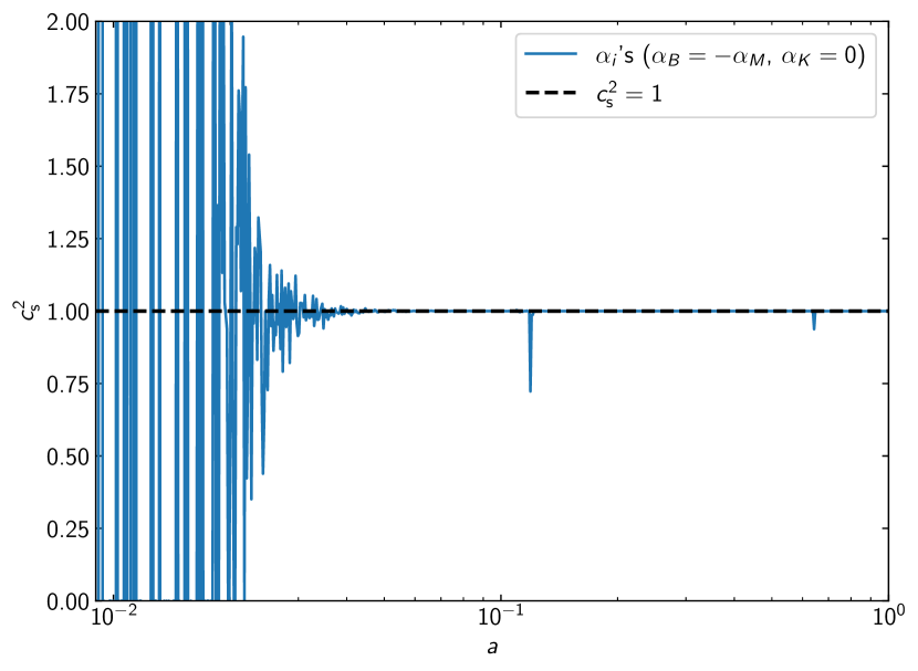
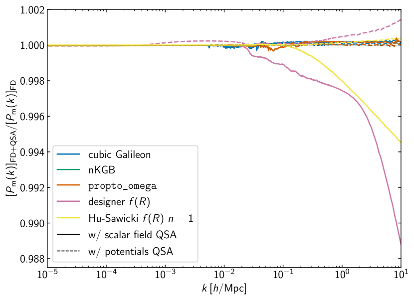
Figure 1: Left: The speed of sound squared, $c_{s}^{2}$, plotted against the scale factor, $a$, for a designer $f(R)$ gravity with $w=-1$ and $B_{0}=0.01$. The blue solid line illustrates the result derived from the Horndeski’s $\alpha_{i}$ functions, the Hubble parameter, and the background densities and pressures (Equation 2). The black dashed line indicates the expected theoretical value of $c_{s}^{2}=1$. The early-time oscillations in the derived quantity are the consequence of cancellation errors further amplified by the small magnitude of $D_{\rm kin}$ in this model. These rapid variations and, more importantly, the violation of the stability condition $c_{s}^{2}>0$ erroneously flag this viable model as unstable, motivating the need for an alternative parametrisation. Right: Effect of the QSA on the $z=0$ matter power spectrum for our test cosmologies. Each line represents the ratio of the matter power spectrum computed by selectively activating the QSA (see discussion in Section 3.1) to that obtained by following the full dynamics (FD) of the scalar field fluctuations. Solid lines indicate the QSA implemented in hi_class, while dashed lines represent the same approach as implemented in MGCAMB. The two QSA strategies are generally consistent, although the methodology based on the metric potentials performs significantly better for the $f(R)$ gravity cosmologies on scales $k\gtrsim 0.1\,h/{\rm Mpc}$.

One challenge when considering the entire class of Horndeski models is their potential for instability in response to perturbations. These instabilities result from unsuitable background solutions, and it is crucial to identify and exclude any parameter combinations leading to such unstable evolution. Physical instabilities come in three kinds (e.g. Hu et al., 2013; Bellini & Sawicki, 2014): (i) gradient instabilities occur when the square of the speed of sound for perturbations turns negative as the background evolves. This negative value can cause perturbations to grow exponentially at small scales, destabilizing them over timescales that are comparable to the cutoff of the theory; (ii) ghost instabilities arise when the sign of the kinetic term for background perturbations is incorrect. This issue is often considered in discussions of quantum stability. If ghost modes are present and dynamically interact, they can destabilize the vacuum, resulting in the production of both ghost and normal modes; (iii) tachyonic instabilities manifest when the effective mass squared of scalar field perturbations is negative, leading to power-law instabilities at large scales growing faster than the Hubble scale. While the absence of ghost and gradient instabilities is an integral requirement for a healthy theory, tachyonic instabilities are not necessarily harmful. In fact, imaginary effective masses can still produce observationally viable models, and considering them as pathological a priori would amount to an overly conservative approach (see Zumalacarregui et al., 2016; Frusciante et al., 2018; Gsponer & Noller, 2021, for different treatments and interpretations of this instability). Here, we will only impose that a theory must be free from ghost and gradient instabilities, which is expressed by the conditions

$$D_{\rm kin}>0,\quad M_{\ast}^{2}>0,\quad c_{\rm s}^{2}>0,\quad\alpha_{\rm B}\neq 2.$$ (22)

Another class of instabilities that can plague Horndeski’s models are the mathematical (or classical) instabilities (Hu et al., 2014), which manifest as exponentially growing modes in the perturbations. The scalar field fluctuations, $V_{X}\equiv a\delta\phi/\phi^{\prime}$, follow the equation of motion

$$\mathcal{A}(\tau)V_{X}^{\prime\prime}+\mathcal{B}(\tau)V_{X}^{\prime}+\left[\mathcal{C}(\tau)+k^{2}\mathcal{D}(\tau)\right]V_{X}=\mathcal{E}(\tau,k)\,,$$ (23)

where the expressions for the time-dependent coefficients, $\{\mathcal{A},\dots,\mathcal{E}\}$, are detailed in Appendix D. To prevent significant growth of unstable modes over cosmological timescales, the following conditions must be satisfied:

• If $\mathcal{B}^{2}(\tau)-4\mathcal{A}(\tau)[\mathcal{C}(\tau)+k^{2}\mathcal{D}(\tau)]>0$:

  $$\frac{-\mathcal{B}(\tau)\pm\sqrt{\mathcal{B}^{2}(\tau)-4\mathcal{A}(\tau)[\mathcal{C}(\tau)+k^{2}\mathcal{D}(\tau)]}}{2\mathcal{A}(\tau)}<\xi H_{0}\,.$$ (24)

• If $\mathcal{B}^{2}(\tau)-4\mathcal{A}(\tau)[\mathcal{C}(\tau)+k^{2}\mathcal{D}(\tau)]<0$:

  $$-\frac{\mathcal{B}(\tau)}{2\mathcal{A}(\tau)}<\xi H_{0}\,.$$ (25)

Here, $\xi$ is a parameter controlling the level of instability in units of the Hubble constant, $H_{0}$, with larger values of $\xi$ allowing models to exhibit faster growing rates of these pathological modes.

For simple fixed-form parametrisations of the $\alpha$-functions (e.g., Equation 20), or even for theories based on a covariant formulation (e.g., Equations 8-13), finding stable models is just a matter of solving for the background evolution and check that the physical (and mathematical) conditions are satisfied. In these scenarios, we must only vary a handful of parameters and the search process is rather efficient. However, for more complex parametrisations producing a wider variety of functional forms, this trial-and-error approach can rapidly become sub-optimal. A mathematically equivalent, yet computationally more advantageous strategy consists in describing the Horndeski’s Lagrangian at the level of background and linear perturbations using a basis that guarantees no-ghost and no-gradient instabilities from the start (Kennedy et al., 2018; Lombriser et al., 2018). In practice, this can be achieved by replacing the $\alpha_{i}$’s with

$$D_{\rm kin},\quad M_{\ast}^{2},\quad c_{\rm s}^{2},\quad\alpha_{B0}\,,$$ (26)

together with the energy density of the scalar field, $\rho_{\phi}$. The initial condition, $\alpha_{B0}\equiv\alpha_{\rm B}(z=0)$, is used to integrate the non-linear differential equation for the braiding

$$\dot{\alpha}_{B}+\left(1-\alpha_{\rm M}+\frac{\dot{H}}{H}\right)\alpha_{\rm B}-\frac{\alpha_{\rm B}^{2}}{2}=\mathcal{S}(x)\,,$$ (27)

where the source term is

$$\mathcal{S}(x)\equiv-2\alpha_{\rm M}+c_{\rm sN}^{2}+\frac{\Delta M_{\ast}^{2}}{M_{\ast}^{2}}\frac{2\dot{H}}{H}-\frac{3(\rho_{\phi}+p_{\phi})}{M_{\ast}^{2}H^{2}}\,,$$ (28)

with the scalar field pressure, $p_{\phi}$, obtained either from the continuity equation (see Appendix D) or, if $w_{\phi}$ is provided, as $p_{\phi}=w_{\phi}\rho_{\phi}$, $c_{\rm sN}^{2}\equiv D_{\rm kin}c_{\rm s}^{2}$, $\Delta M_{\ast}^{2}\equiv M_{\ast}^{2}-1$, and $\alpha_{\rm M}$ given by Equation (3). Note that Equation (27) follows from Equation (2) after expressing $H^{\prime}$ in terms of the density and pressure of the matter and scalar fields, and upon transforming conformal time derivatives into derivatives with respect to $\ln a$. Once a solution for $\alpha_{\rm B}$ is found, the kineticity, $\alpha_{\rm K}$, can be derived from Equation (6).

It has been argued that stable basis functions offer no distinct advantages over the standard $\alpha$-functions in terms of computational efficiency or modeling capabilities (e.g., Denissenya & Linder, 2018). Contrary to this, our work suggests that reformulating Horndeski’s gravity using the stable basis, Equation (26), enhances our ability to efficiently sample viable theories and improves numerical stability. The left panel of Figure1 illustrates how parametrisation with the $\alpha$-functions might misclassify models as unstable. Specifically, designer $f(R)$ gravity on a $\Lambda$CDM background, which is inherently stable ($c_{\rm s}^{2}=1$), shows rapid variations in the speed of sound due to inexact numerical cancellations when using Equation (2), violating the no-gradient condition multiple times. In contrast, the stable basis directly incorporates the speed of sound as an input function, which, in this example, remains constant at unity throughout. Furthermore, using physically motivated parametrisations of the stable basis functions alongside highly optimised root finders and fast integrators (such as those implemented in modern Einstein-Boltzmann solvers) typically leads to rapid converge towards a solution for the braiding with the expected early-time evolution (see Section 5 for details). Depending on the complexity of the parameter space, iteratively solving a differential equation is often more efficient than searching for a stable model starting from the $\alpha$-functions.

2.2 Quasi-static approximation

The quasi-static approximation (QSA) is key to the study of cosmological perturbations within modified gravity and dark energy models. This approximation rests on the premise that the primary timescale of influence is the Hubble rate, and on scales smaller than the sound horizon ($c_{\rm s}^{2}k^{2}\gg a^{2}H^{2}$) the time derivatives of the scalar field perturbations can be neglected owing to the rapid response of this degree of freedom to changes in the system. This simplifies the equations of motion for the scalar field into algebraic constraints, thus offering substantial computational benefits. In particular, for large values of the effective mass (i.e. the term proportional to $V_{X}$ in Equation 23) the scalar field perturbations undergo high-frequency oscillations that necessitate small integration steps. These can slow down computations significantly or even cause the solver to stall when the step size falls below machine precision. By employing the QSA, we can focus on the secular evolution of these perturbations, effectively excluding the high-frequency components.

However, the QSA must be applied with care depending on the scale and the specific dynamics of the model. Einstein-Boltzmann solvers like MGCAMB (Hojjati et al., 2011; Zucca et al., 2019b; Wang et al., 2023) and mgclass (Sakr & Martinelli, 2021) employ this approximation across all scales and throughout the entire evolution of the perturbations – an approach that can potentially affect the accuracy of the predictions on large scales (Sawicki & Bellini, 2015). At the other end of the spectrum are solvers like EFTCAMB (Hu et al., 2013) that avoid using the QSA entirely, a choice that can significantly degrade performance, in particular for certain sub-classes of models. The hi_class solver (Zumalacarregui et al., 2016; Bellini et al., 2019) adopts a hybrid strategy that leverages the computational efficiency of the QSA along with the accuracy provided by the full scalar field dynamics. Within this scheme, the QSA is selectively activated or deactivated for each time and scale individually, ensuring its use is optimized. The scalar field fluctuations and their time derivatives can be read off Equation (23) once the terms proportional to $V_{X}^{\prime\prime}$ and $V_{X}^{\prime}$ are neglected,

$$V_{X} =\frac{\mathcal{E}(\tau,\,k)}{\mathcal{C}(\tau)+k^{2}\mathcal{D}(\tau)}\,,$$ (29a)

$$V^{\prime}_{X} =\frac{{\rm d}}{{\rm d}\tau}\left[\frac{\mathcal{E}(\tau,\,k)}{\mathcal{C}(\tau)+k^{2}\mathcal{D}(\tau)}\right]\,.$$ (29b)

It should be noted that, even within the quasi-static regime, $V_{X}$ remains time-dependent, implying that its time derivative does not vanish. Consequently, terms proportional to $V^{\prime}_{X}$ (or time derivatives of other metric perturbations) in the Einstein equations, which are typically not reduced by small coefficients, must be accounted for in our calculations.

Although the QSA implemented through Equation (29) provides a good description of the scalar field fluctuations and their derivatives, it can lead to small-scale inaccuracies in the matter perturbations for some models. This is illustrated in the right panel of Figure 1, where the matter power spectrum for two of our test $f(R)$ gravity models (pink and yellow solid lines), computed by selectively activating the QSA in hi_class, deviates by up to 1% for $k\gtrsim 0.1\,h/\text{Mpc}$. For analyses restricted to the linear regime, these deviations are negligible. However, the linear power spectrum is also used as input for methods that predict non-linear structure formation (e.g., Bose & Koyama, 2016; Aviles & Cervantes-Cota, 2017; Cusin et al., 2017; Cataneo et al., 2018; Giblin et al., 2019; Valogiannis et al., 2019), and such small-scale inaccuracies can propagate to observables probing the non-linear regime, potentially exceeding the accuracy requirements established for Stage IV surveys (e.g., Taylor et al., 2018).

A different QSA strategy consists in working directly with the modified metric potentials (Bloomfield et al., 2012; Pace et al., 2020). In the Newtonian gauge, the linearised modified Einstein field equation for the Newtonian potential, $\Psi$, and the intrinsic spatial curvature, $\Phi$, read (Zhao et al., 2008; Hojjati et al., 2011)

$$k^{2}\Psi=-\frac{3}{2}\mu(a,k)a^{2}\left[\rho_{\rm m}\Delta_{\rm m}+3(\rho_{\rm m}+p_{\rm m})\sigma_{\rm m}\right],$$ (30a)

$$k^{2}[\Phi-\gamma(a,k)\Psi]=\frac{9}{2}\mu(a,k)a^{2}(\rho_{\rm m}+p_{\rm m})\sigma_{\rm m}\,,$$ (30b)

where the total comoving-gauge density perturbations are summed over all matter species $I\in\{\text{c, b},\text{r},\nu,\dots\}$, $\rho_{\rm m}\Delta_{\rm m}\equiv\sum_{I}\rho_{I}\Delta_{I}$, with $\Delta_{I}$ being the comoving density contrast for the species $I$, and $(\rho_{\rm m}+p_{\rm m})\sigma_{\rm m}\equiv\sum_{I}(\rho_{I}+p_{I})\sigma_{I}$ with $\sigma_{I}$ denoting the anisotropic stress of the individual matter fluids. Changes to the gravitational coupling experienced by non-relativistic particles are encoded in $\mu$, while the gravitational slip, $\gamma$, sources differences between the two metric potentials also in the absence of anisotropic stress. General Relativity is recovered for $\mu=\gamma=1$.

For the Horndeski’s models described by the Lagrangian in Equation (5) the two phenomenological functions take the simple forms (Pogosian & Silvestri, 2016)

$$\mu(k,a)=\frac{1}{M_{\ast}^{2}}\frac{\mu_{\rm p}+k^{2}c_{\rm sN}^{2}M_{\ast}^{2}\mu_{\infty}/a^{2}H^{2}}{\mu_{\rm p}+k^{2}c_{\rm sN}^{2}/a^{2}H^{2}}\,,$$ (31a)

$$\gamma(k,a)=\frac{\mu_{\rm p}+k^{2}c_{\rm sN}^{2}M_{\ast}^{2}\mu_{Z,\infty}/a^{2}H^{2}}{\mu_{\rm p}+k^{2}c_{\rm sN}^{2}\mu_{\infty}/a^{2}H^{2}}\,,$$ (31b)

consistent with the notation of Pace et al. (2020). Definitions for the quantities $\{\mu_{\rm p},\mu_{\infty},\mu_{Z,\infty}\}$ are detailed in Appendix D. The extension of hi_class introduced in this work, mochi_class, bypasses the QSA formulation from Equation (29) in favor of Equations (30) and (31) in synchronous gauge, similar to MGCAMB. However, it activates the QSA selectively based on scale and time, when the scalar field’s effective mass and the discrepancy between full and quasi-static solutions meet specific user-defined criteria (see Bellini et al., 2019, and Section 3 for details). The dashed lines in the right panel of Figure 1 demonstrate that the QSA approach implemented through the metric potentials is less affected by the neglected dynamics of the scalar field fluctuations compared to the implementation using Equation (29).

3 Code structure and implementation

The code developed for this study, mochi_class, builds on hi_class, which itself extends the capabilities of the Einstein-Boltzmann solver class (Blas et al., 2011; Lesgourgues & Tram, 2011) to evolve the background and linear perturbations of scalar-tensor theories within the Horndeski’s framework. This section explores the new features introduced in mochi_class. For a comprehensive review of the functionalities in hi_class we refer the reader to Zumalacarregui et al. (2016); Bellini et al. (2019).

mochi_class enhances hi_class by modifying the input, background, and perturbations modules to ensure greater numerical stability and facilitate a more comprehensive investigation of Horndeski’s gravity. In the following, we provide a detailed description of these modifications.

3.1 Input and precision parameters

By setting the gravity_model variable to stable_params, users can specify a path to a file containing the functions $\Delta M_{\ast}^{2}$, $D_{\rm kin}$, and $c_{\rm s}^{2}$, as well as the $\ln a$ sampling times, using smg_file_name. Alternatively, these quantities can be directly assigned to the corresponding code variables: Delta_M2, D_kin, cs2, and lna_smg. This direct assignment method is particularly recommended when running mochi_class via the classy Python wrapper. To mitigate the impact of interpolation errors within the computational pipeline, we recommend using a time-sampling step size no larger than $\Delta\ln a=7.5\times 10^{-4}$ for the range $\ln a\in[-2,0]$. In mochi_class, the hi_class variable parameters_smg serves a container for the initial condition, $\alpha_{B0}$.

Users must also select an expansion_model to define the background evolution of the scalar field. They can choose from the two hi_class analytic expansion models, {lcdm, w0wa}, or opt for the new non-parametric models {wext, rho_de}. In the wext model, the scalar field background density is integrated using the continuity equation (Equation 43), with the background pressure defined as $p_{\phi}=w_{\phi}\rho_{\phi}$. For the rho_de model, the approach starts with the normalised background density $\tilde{\rho}_{\phi}\equiv\rho_{\phi}/\rho_{\phi}(z=0)$, which is transformed to $\rho_{\phi}=\Omega_{\phi}H_{0}^{2}\tilde{\rho}_{\phi}$. Here, the Hubble constant is an input parameter, and $\Omega_{\phi}=1-\sum_{I}\Omega_{I}$ represents the present-day normalised background energy-density in a flat universe. The scalar field background pressure in this configuration is then computed as

$$p_{\phi}=-\rho_{\phi}-\frac{\dot{\rho}_{\phi}}{3}\,.$$ (32)

It is important to note that hi_class employs a root-finding algorithm to determine the value of a user specified parameter necessary to achieve the present-day energy density, $\Omega_{\phi}H_{0}^{2}$ (see Section 3.3 in Bellini et al., 2019). It can be the initial conditions of the scalar field, $\phi(\tau_{\rm ini})$, its time derivative, $\phi^{\prime}(\tau_{\rm ini})$, or any other parameter that contributes to the energy density of the scalar field. This step is essential for models based on a covariant Lagrangian where $\rho_{\phi}$ is not known in advance, requiring the cosmological background to be solved self-consistently with the scalar field and the $\alpha$-functions. However, this becomes redundant in cases where the scalar field energy-density evolution is predefined, as often happens in the effective-theory approach. To optimize computational efficiency, mochi_class has been modified to bypass the root-finding process. Instead, it directly uses $\Omega_{\phi}$ from the closure relation, $\Omega_{\rm tot}=1$, to rescale the normalized energy density, $\tilde{\rho}_{\phi}$.

Similarly to the stable basis functions, wext and rho_de can read the necessary data either from a text file containing two columns {$\ln a$, $w_{\phi}$ or $\tilde{\rho}_{\phi}$} located at a path specified in expansion_file_name, or directly from input arrays lna_de and de_evo. To minimise interpolation errors, it is recommended to use a time-sampling step-size $\Delta\ln a\leq 7.5\times 10^{-4}$ for the range $\ln a\in[-2,0]$. In addition, when utilizing mochi_class, users must activate the GR approximation scheme (see Section 3.3 below) by setting method_gr_smg = on. This feature allows the code to solve the standard system of equations down to a user-specified redshift, z_gr_smg. Given our focus on late-time modifications to GR, the default value for this transition epoch is set deep within the matter-dominated era, specifically at $\texttt{z\_gr\_smg}=99$.

While the stable basis in mochi_class ensures the positivity of the de-mixed kinetic term, the Planck mass, and the speed of sound, it does not automatically guarantee that the condition $\alpha_{B}\neq 2$ from Equation (22) is met, as this requires a solution for the braiding first. Therefore, we can safely set skip_stability_tests_smg = yes, as mochi_class always tests that the braiding never crosses 2, which was not implemented in hi_class. Furthermore, setting skip_math_stability_smg = no allows the code to check for exponentially growing modes by enforcing the mathematical stability conditions outlined in Equations (24) and (25). Users can control the allowed instability growth rate via the exp_rate_smg variable, which defaults to 1.

Similar to hi_class, mochi_class has the option to treat the scalar field as a dynamical degree of freedom throughout the perturbations’ evolution, or to apply the QSA whenever is safe to do so. These configurations can be selected by setting the method_qs_smg input variable to fully_dynamic for the former, or automatic for the latter. In automatic mode, the QSA is activated for specific time intervals and wavenumbers based on whether the effective mass of the scalar field exceeds the threshold trigger_mass_qs_smg, and the amplitude of scalar field fluctuations has reduced by a factor defined in eps_s_qs_smg (Bellini et al., 2019). Default values are set at trigger_mass_qs_smg = 100 and eps_s_qs_smg = 0.01, which, even for large departures from the standard cosmology, affect the computed power spectra by $\lesssim 0.1\%$. mochi_class can accurately solve the quasi-static equations down to $z=0$ (see Section 2.2), eliminating the need to enforce the full dynamic of the scalar field at low redshifts. Consequently, the corresponding control variable z_fd_qs_smg can be safely set to 0.

mochi_class also includes new precision parameters. Below is a list describing their scope and default values:

• background_Nloga_smg and loga_split: the background time-sampling strategy adopted for $a\gtrsim 0.05$ is crucial for achieving accurate interpolation of the quasi-static quantities $\{\mu_{\rm p},\mu_{\infty},\mu_{Z,\infty}\}$. To this end, mochi_class employs a denser sampling for $\ln a>\texttt{loga\_split}$, with the number of points controlled by background_Nloga_smg. For $\ln a<\texttt{loga\_split}$ the number of sampling points reverts to the standard set by the class precision variable background_Nloga. The default settings are background_Nloga = 3000, background_Nloga_smg = 3000, and loga_split = -3.

• eps_bw_integration_rho_smg: when using the expansion_model = wext, where users define the equation of state for the scalar field, its background density is calculated from the continuity equation. This equation is integrated from $a=1$ down to the scale factor $(1-\texttt{eps\_bw\_integration\_rho\_smg})/(1+\texttt{z\_gr\_smg})$. To ensure smooth derivatives of the scalar field pressure and related quantities at z_gr_smg, the default setting for eps_bw_integration_rho_smg is 0.1.

• eps_bw_integration_braid: the equation for the braiding, Equation (27), is integrated from $a=1$ backward to the scale factor $(1-\texttt{eps\_bw\_integration\_braid})/(1+\texttt{z\_gr\_smg})$. To ensure smoothness at z_gr_smg for all functions derived from $\alpha_{\rm B}$ and its derivatives, we recommend setting eps_bw_integration_braid to at least 0.1.

• tol_background_bw_integration: this variable governs the integration accuracy of the continuity equation, Equation (43), and of the braiding equation, Equation (27). Based on our analysis, setting tol_background_bw_integration = 1e-10 provides a good balance between computational speed and solution accuracy across all models examined in this study.

• braid_activation_threshold: Solving Equation (27) into the matter-dominated epoch poses numerical challenges, particularly for models that rapidly converge to GR at early times. While inaccuracies at high redshifts generally do not impact the late-time modified gravity phenomenology, they can introduce spurious instabilities that may incorrectly render a model non-viable. To minimize these effects, modifications to the Einstein equations are triggered only when the braiding solution reaches the braid_activation_threshold. Practically, this means adjusting the transition redshift, z_gr_smg, to match the redshift at which $|\alpha_{\rm B}|$ first equals braid_activation_threshold. Note that this threshold is not enforced for models with $|\alpha_{B0}|\leq\texttt{braid\_activation\_threshold}$, e.g. quintessence and k-essence. The default value of braid_activation_threshold = 1e-12 is chosen to ensure precise predictions across the broad range of deviations from GR examined in this study.

• dtau_start_qs: at the onset of modified gravity, marked by z_gr_smg, mochi_class introduces the scalar field as a new degree of freedom by incorporating the equation for the field fluctuations (Equation 23) and its couplings to the metric perturbations into the Einstein-Boltzmann system. Initial conditions are defined by the QSA outlined in Equation (29). The code then waits a conformal time specified by dtau_start_qs before assessing whether to activate the QSA, effectively turning the scalar field fluctuations into algebraic constraints. We found that dtau_start_qs = 1e-7 works well for all models tested.

3.2 Background

Once the input arrays are prepared, the initial step involves calculating the background density of the scalar field. Depending on the chosen expansion model, the code performs one of the following actions: (i) integrates the continuity equation and stores both $\rho_{\phi}$ and $p_{\phi}$ for later use; (ii) rescales the input normalized background energy-density of the scalar field to compute $\rho_{\phi}$, and calculates $p_{\phi}$ using Equation (32), saving both values for future reference; (iii) analytically determines the scalar field density and pressure, along with other background quantities, as already implemented in hi_class.

Subsequently, with access to the stable basis functions, the scalar field density and pressure, as well as $H$ and $\dot{H}$, the code solves for $\alpha_{\rm B}$ by backward integrating Equation (27) from its present-day value, $\alpha_{B0}$. It calculates the kineticity, $\alpha_{\rm K}$, using Equation (6), and if necessary updates z_gr_smg based on the braid_activation_threshold. However, it is important to acknowledge a slight inconsistency in our approach: $\rho_{\phi}$, $p_{\phi}$, and associated variables are not recalculated for the interval between the newly adjusted and the original z_gr_smg values to accommodate a lower transition redshift. This methodological choice is made to save computational resources while only introducing a marginal error in MG models that rapidly converge to GR. Within the Horndeski’s framework we expect changes to the growth of structure to be linked to changes to the background expansion. Therefore, viable models exhibiting significant departures from standard gravity only in recent epochs, presumably also closely match a $\Lambda$CDM expansion history until recently.

Finally, with all relevant background functions now available, mochi_class computes the quasi-static quantities $\{\mu_{\rm p},\mu_{\infty},\mu_{Z,\infty}\}$ and their derivatives. These are also stored in the background table and forwarded to the perturbations module for further processing.

3.3 Perturbations

The evolution of the perturbations closely follows that implemented in hi_class, except for the new GR approximation scheme and the effective field equations used for the QSA. While hi_class follows the dynamics of the scalar field and its coupling to the metric tensor already prior to recombination, mochi_class activates the additional degree of freedom only after the time z_gr_smg. This is achieved by enabling method_gr_smg, which directs the solver to apply the standard class equations up to the transition redshift.

Once the GR approximation is deactivated, the initial conditions for the scalar field are derived from the quasi-static expressions given in Equation (29), transitioning from the standard class equations to those of hi_class. This approximation scheme is crucial to manage the discontinuity at z_gr_smg, which otherwise leads to computational instability by forcing the integrator to attempt reductions in the step size to below double precision levels. Consistent with other approximation schemes used, the initial conditions for the metric and stress-energy tensor perturbations are set from the integration time step immediately preceding the deactivation.

With the initial conditions now defined, mochi_class can use the QSA scheme of hi_class for the evolution of the perturbations. Should the scalar field effective mass and fluctuations amplitude satisfy specific criteria (Bellini et al., 2019), the QSA may be selectively activated or deactivated up to six times. However, within mochi_class, this scheme is only applicable to each wavenumber, $k$, following a designated time, $\tau(\texttt{z\_gr\_smg})+\texttt{dtau\_start\_qs}$. Furthermore, rather than applying the QSA directly to the scalar field fluctuations, $V_{X}$, mochi_class targets the metric potentials, thereby enhancing numerical accuracy. Accordingly, the quasi-static part of hi_class has been restructured to align with the methodology developed for MGCAMB.

4 Code validation and performance

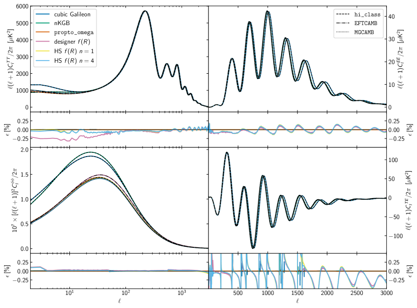
Figure 2: Comparison of the CMB auto- and cross-power spectra as computed by mochi_class (colored lines) against predictions from well-validated Einstein-Boltzmann solvers (black lines). The dashed lines for cubic Galileon and nKGB models, as well as propto_omega, are generated by hi_class following the full scalar field dynamics. For designer $f(R)$ gravity, the dot-dashed lines are obtained with EFTCAMB, while the dotted lines for Hu-Sawicki (HS) $f(R)$ models are produced by MGCAMB using the quasi-static approximation. The fractional differences, $\epsilon$, shown in the lower sub-panels quantify the agreement between mochi_class in automatic mode and the reference spectra obtained with the other Einstein-Boltzmann solvers. Notably, all discrepancies are below 0.25% except in the TE cross-spectra, where the reference spectra’s zero crossings amplify the deviations. All discrepancies larger than 0.05% for the $f(R)$ models stem primarily from differences between class and CAMB, and are also present in $\Lambda$CDM (not shown).

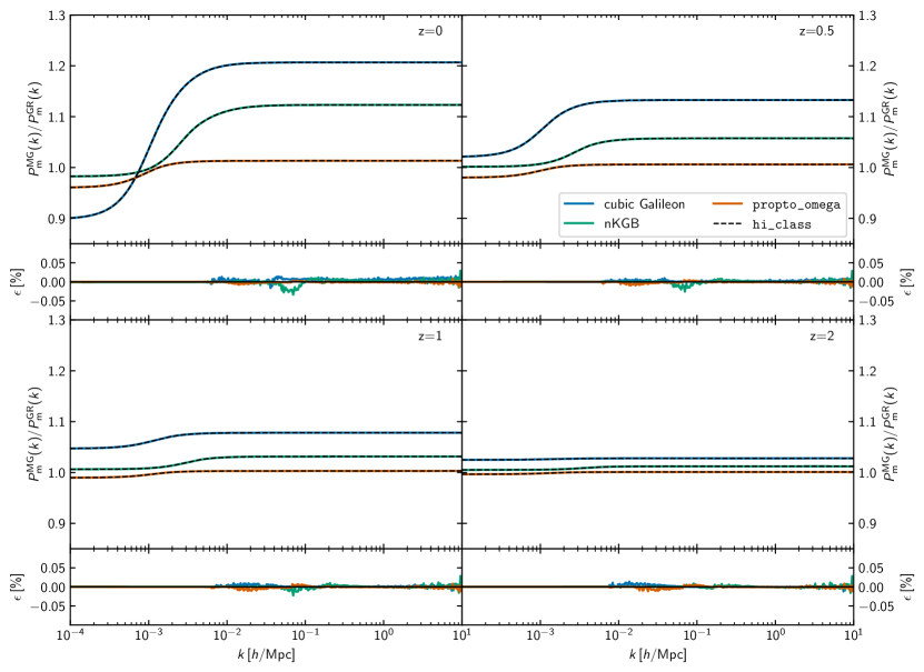
Figure 3: mochi_class accuracy quantification for the matter power spectrum through comparison with hi_class across various redshifts ($z=0,0.5,1,2$). Each main panel displays the matter power spectrum ratio in modified gravity models relative to $\Lambda$CDM as calculated by mochi_class (colored lines) and hi_class (dashed lines). The sub-panels show the fractional deviation of mochi_class from hi_class, indicating an agreement within 0.05% for the considered redshifts. This level of accuracy demonstrates the robustness of the computational strategy adopted in mochi_class, which includes an alternative parametrisation of the Horndeski’s functions, a QSA formulated in terms of modifications to the equations for the metric potentials, and the activation of modified gravity deep into the matter-dominated era.

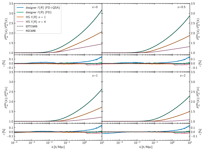
Figure 4: Extending Figure 3, here we consider modified gravity models characterised by a scale-dependent growth on sub-horizon scales. The reference power spectra for $f(R)$ gravity are computed with EFTCAMB (dashed) and MGCAMB (dotted). The lower panels focus on the fractional deviation of mochi_class from the CAMB-based solvers, providing a direct comparison for the matter power spectrum ratios shown above. The Hu-Sawicki (HS) models demonstrate a close match, with deviations from MGCAMB remaining under 0.025% across all scales. In contrast, for the designer $f(R)$ model, mochi_class shows a consistent discrepancy that increases at smaller scales (blue line), a result predominantly due to the quasi-static approximation. This difference, in fact, significantly reduces when mochi_class always integrates the full scalar field dynamics (green line).

Before exploring the new capabilities of mochi_class, we first compare its predictions with those from established codes such as hi_class (Zumalacarregui et al., 2016; Bellini et al., 2019), EFTCAMB (Hu et al., 2013, 2014), and MGCAMB (Hojjati et al., 2011; Zucca et al., 2019b; Wang et al., 2023). This comparative analysis allows for a thorough assessment of all test models and ensures the robustness of our results across different parametrisations, approximations, and integration strategies. Although not discussed here, similar agreements between mochi_class and the other Einstein-Boltzmann solvers are achieved when including massive neutrinos. This is especially true for the small, non-factorisable contributions to the growth of structure caused by their coupling to modified gravity.

4.1 CMB spectra

Figure 2 displays the CMB multipoles for temperature (upper left), polarization (upper right), their cross-correlation (lower right), and the lensing potential power spectrum (lower left). The lower sub-panels contain the relative deviations of the mochi_class predictions (coloured lines) compared to the results from other Einstein-Boltzmann solvers (black lines). As reference spectra, we use hi_class without the QSA for cubic Galileon, nKGB, and propto_omega models; EFTCAMB for designer $f(R)$ gravity; and MGCAMB for Hu-Sawicki $f(R)$ gravity. These quantities were generated using the precision settings detailed in Appendix A for both CAMB and class.

First, it is important to note that the differences between mochi_class and hi_class are barely visible at this scale. This suggests that the newly implemented GR approximation at early times, the reparametrisation using stable basis functions, and the application of the quasi-static approximation until late in the perturbation evolution, all introduce minimal numerical errors.

The agreement between mochi_class and the CAMB-based codes is very good, with differences remaining well within $\sim 0.25\%$. Further analysis reveals that mismatches exceeding 0.05% come from variations between class and CAMB, similarly affecting $\Lambda$CDM predictions (not shown). This validates the QSA implementation in mochi_class, which closely aligns with MGCAMB, and confirms the reliability of the QSA/full dynamics switching feature in hi_class. Note that despite EFTCAMB and MGCAMB both deriving from CAMB, discrepancies around 0.2% are observed between these codes for the low-$\ell$ temperature multipoles. Initially, these could be attributed to the activation of the QSA in mochi_class, potentially affecting the accuracy of the integrated Sachs-Wolfe (ISW) effect calculations, particularly in the designer $f(R)$ model where deviations from GR are more pronounced. However, further investigation indicated that these differences are due to the use of different CAMB versions, with MGCAMB employing a more recent release.

4.2 Matter power spectrum

Figure 3 presents the evolution of the matter power spectrum ratio, $P_{\rm m}^{\rm MG}(k)/P_{\rm m}^{\rm GR}(k)$, for the three cosmologies characterised by scale-independent growth on sub-horizon scales. The lower sub-panels show that for these models mochi_class (coloured lines) deviates by an average of approximately $0.01\%$ from hi_class (black lines). Differences are negligible for scales $k\lesssim 0.01\,h/{\rm Mpc}$, where the QSA is never activated.

To isolate the impact of the new mochi_class features, Figure 4 also shows the matter power spectrum of the $f(R)$ gravity predictions relative to same quantity in $\Lambda$CDM. For the Hu-Sawicki models the agreement between mochi_class (coloured lines) and MGCAMB (dotted lines) is excellent across all redshifts. Differences larger that 0.2% are visible only for $k\gtrsim 1\,h/{\rm Mpc}$, regardless of model and time. Using an independent Mathematica notebook employing the QSA, we have verified that these small differences originate from MGCAMB.

Moreover, Figure 4 illustrates the (albeit small) inaccuracies introduced by the QSA in the designer model. The blue lines, generated using a hybrid method that activates the QSA under certain conditions (detailed in Section 3), should be compared with the EFTCAMB predictions (dashed lines), which do not employ the QSA. As expected, the small scales are most affected by this approximation, due to the conditions for its activation being met for more extended time intervals. To verify that deviations from EFTCAMB are caused by the QSA, we forced mochi_class to follow the full dynamics of the scalar field (green line). The lower sub-panels confirm that mochi_class predictions now align with EFTCAMB at a level of $10^{-4}$.

4.3 Performance

	input (I)	background (B)	perturbations (P)	(I)+(B)+(P)	total
Cubic Galileon	-80%	+100%	-52%	-52%	-40%
propto_omega	-75%	+100%	-25%	-24%	-17%

Table 1: Variations in execution time for the input (I), background (B), and perturbations (P) modules in mochi_class, relative to hi_class. Both codes used the automatic mode, with hi_class forcing full dynamical evolution of the scalar field from $z=10$, as recommended by its developers. The models considered—Cubic Galileon, based on the covariant Lagrangian, and propto_omega, based on effective theory—are representative of the two approaches implemented in hi_class. The column labeled (I)+(B)+(P) lists the cumulative variations across the three modules, emphasising that the evolution of the perturbations is the primary bottleneck. The final column indicates that, overall, enabling the QSA at low redshifts can lead to substantial performance improvements, with minimal impact on accuracy (see Figure 1).

Here we assess the impact of the mochi_class patch on execution time, examining both individual modules and the overall runtime. Table 1 summarises the relative changes in execution time compared to hi_class for the input, background, and perturbations modules, as well as their combined effect and the total runtime variation, including the other unmodified modules. To ensure a fair comparison, we evaluate two models that activate different features in hi_class: the cubic Galileon model, which requires preparatory steps to iteratively determine suitable initial conditions and map the Horndeski $G_{i}$’s to the $\alpha$-basis, and the propto_omega model, which involves direct analytic expressions for both the $\alpha$’s and the scalar field background evolution.

Contrary to intuition, mochi_class shows reduced runtime for both models at the input level, despite propto_omega only needing to fill the relevant arrays. This is because hi_class unnecessarily applies the root finder for the initial conditions to this model–a step not performed by mochi_class. Unsurprisingly, the execution of the background module takes twice as long as in hi_class, due to the integration of the differential equation for the braiding function. However, this slowdown is less severe than suggested by Denissenya & Linder (2018). Assuming a uniform scanning strategy of their two-dimensional parameter space and a stable region amounting to 22% of the prior volume, the number of unstable models is 3.5 times that of the viable models. Therefore, starting from the stable basis ensures an overall 56% speedup for the background module compared to using the $\alpha$-functions in this particular scenario. This efficiency gap becomes even wider for complex parametrisations, such as those discussed in Section 5, where stable models can be particularly challenging to find.

The third column of Table 1 highlights the advantage of enabling the QSA for $z<10$: it can reduce the computing time for the evolution of perturbations by up to 50%. Since this part of the code contributes most significantly to the cumulative execution time of the three modified modules (fourth column), any performance improvement here directly impacts the total runtime of the Einstein-Boltzmann solver (last column). The difference between the two codes arises from enabling the activation of the QSA in mochi_class throughout the perturbation evolution, while in hi_class we apply it only up to some high redshift (i.e., $z=10$), as recommended by its developers.

5 Extended Parametrisation for Horndeski gravity

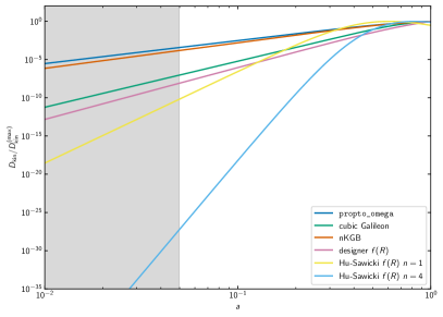
Figure 5: Evolution of the de-mixed kinetic term, $D_{\rm kin}$, normalised to its maximum value, $D_{\rm kin}^{\rm(max)}$, across a variety of modified gravity theories. At sufficiently early time (shaded area) $D_{\text{kin}}$ closely follows a power-law behavior for all models. A similar behavior (not shown) characterises departures from the cosmological strength of gravity, $\Delta M_{\ast}^{2}$, and the background energy density of the scalar field, $\rho_{\phi}$.

After establishing mochi_class accuracy and efficiency using extensively studied modified gravity cosmologies, we can now leverage its new features to input general functions of time and explore the phenomenology of Horndeski gravity in greater detail. For this purpose, a parametrisation that generalises propto_omega and includes all covariant theories analysed in Section 3 could be extremely valuable (Linder, 2016).

A common feature of all our test models is that, deep in the matter-dominated era, their stable basis functions either approach the GR limit as power laws, $A_{J}a^{\zeta_{J}}$, or tend to constant values, $C_{J}$, to a very good approximation. For instance, Figure 5 illustrates that, regardless of the specifics governing the dynamics of the scalar field, the de-mixed kinetic term is well described by a power law for $a\lesssim 0.05$ (shaded area). Therefore, any late-time evolution of the stable functions can be interpreted as deviations, $\Delta_{J}$, from this early-time power-law behavior. Specifically, we can express the stable functions as

$$\Delta M_{\ast}^{2} =\operatorname{sgn}(A_{M})e^{\zeta_{M}\cdot x+b_{M}+\Delta_{M}(x)}\,,$$ (33a)

$$D_{\rm kin} =e^{\zeta_{D}\cdot x+b_{D}+\Delta_{D}(x)}\,,$$ (33b)

$$c_{\rm s}^{2} =\left[\operatorname{sgn}(A_{c_{\rm s}})e^{\zeta_{c_{\rm s}}\cdot x+b_{c_{\rm s}}}+C_{c_{\rm s}}\right]e^{\Delta_{c_{\rm s}}(x)}\,,$$ (33c)

$$\tilde{\rho}_{\phi} =\left[\operatorname{sgn}(A_{\rho})e^{\zeta_{\rho}\cdot x+b_{\rho}}+C_{\rho}\right]\Delta_{\rho}(x)\,,$$ (33d)

where $x\equiv\ln a$, $b_{J}\equiv\ln|A_{J}|$, $\operatorname{sgn}$ denotes the sign function, and for $x\ll 0$ we have the limiting values

$$\Delta_{M},\Delta_{D},\Delta_{c_{\rm s}} \rightarrow 0\,,$$ (34a)

$$\Delta_{\rho} \rightarrow 1\,.$$ (34b)

The constant $C_{\rho}$ is not a free parameter; it is determined by the constraint $\tilde{\rho}_{\phi}(x=0)=1$. For negative $A_{M}$ and $A_{c_{\rm s}}$, we must ensure that $\Delta M_{\ast}^{2}>-1$ and $c_{\rm s}^{2}>0$ throughout the evolution. Given that the power-law term for the speed of sound generally represents a small correction to the constant $C_{c_{\rm s}}$ (as discussed below), it can be neglected when generating new models. Therefore, the gradient-free condition implies simply that $C_{c_{\rm s}}>0$.

5.1 Parametrising departures from constants and power laws

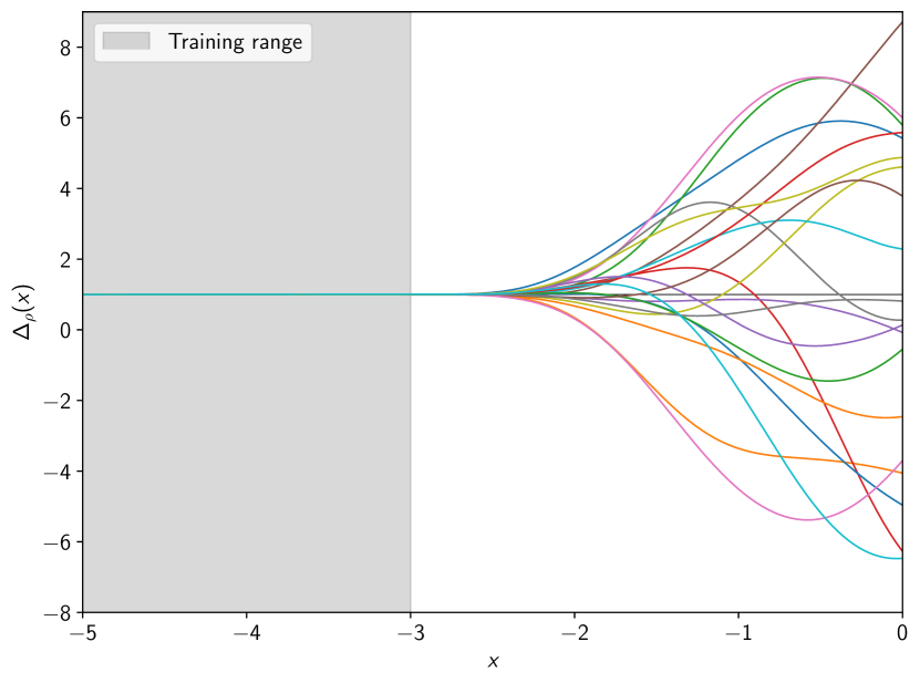
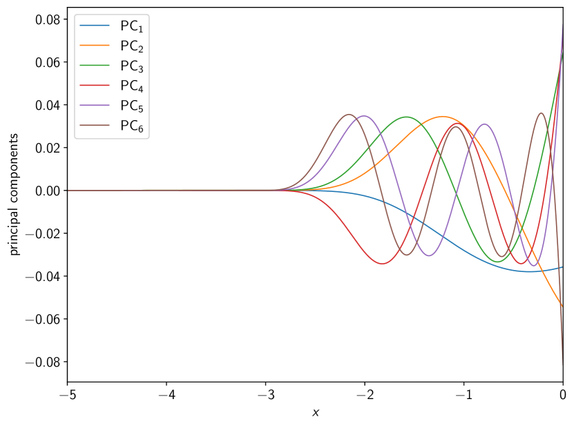
Figure 6: Left: Samples from a Gaussian Process (GP) representing the correction factor, $\Delta_{\rho}$, which quantifies deviations in the scalar field background energy-density from a baseline power-law behavior as a function of time, $x\equiv\ln a$. The GP’s hyper-parameters are detailed in the main text, and its mean is set to 1. The shaded region marks the training range, over which the GP is constrained to unity, coinciding with the interval where the background energy-density of the scalar field closely follows a power-law behaviour. The various trajectories of the 20 curves outside the training range represent possible extrapolations of $\Delta_{\rho}$ beyond the power-law regime. Right: The first six principal components (PCs) extracted from 10,000 samples generated by the Gaussian Process described in the left figure. The PCs illustrated here are sufficient to reconstruct the scalar field background energy-density of all test models to better than 1%, thus demonstrating the efficiency of the dimensionality reduction achieved by the principal component analysis (PCA). Similar performance apply to PCAs for the other input functions within the stable basis.

Next, we need to find a sufficiently general yet simple parametrisation for the functions $\Delta_{J}$. A commonly employed strategy to parametrise the EFT functions or the $\alpha_{i}$’s involves expanding them as ratios of polynomials, i.e., Padé approximants (see, e.g., Gleyzes, 2017; Peirone et al., 2017). Here, we opt for an alternative methodology grounded in Gaussian Processes (GPs) (see, e.g., Rasmussen & Williams, 2006; Aigrain & Foreman-Mackey, 2022, for detailed discussions) and Principal Component Analysis (PCA). In broad terms, we proceed as follows:

1. We generate training data such that the GP is consistent with Equation (34). Practically, this requires an array of zeroes over the interval $x\in[-5,-3]$.

2. After choosing values for the hyperparameters defining the GP kernel, $K(x_{i},x_{j})$, for a particular basis function, we let the GP learn from the training data. Note that all our GPs have zero mean.

3. We draw thousands of samples from the trained GP, calculate their mean, and subtract it from each sample so that the transformed samples have zero mean.

4. We perform PCA on the transformed samples and retain the first $N_{J}$ principal components.

5. We project the specific basis function of each test model (cubic Galileon, nKGB, etc.) onto the selected principal components and quantify the accuracy of the reconstructed approximation.

6. For each basis function, we iterate over steps 2-5 to find the hyperparameter values and number of principal components that provide percent-level reconstruction accuracy for $x>-3$.

It is reasonable to assume that a covariant theory of gravity in the Horndeski class should be described by basis functions that vary smoothly with time. This assumption restricts the choice of the GP kernel to either the squared exponential form,

$$K(x_{i},x_{j})=\sigma^{2}\exp\left[-\frac{(x_{i}-x_{j})^{2}}{2\ell^{2}}\right]\,,$$ (35)

or the rational quadratic form,

$$K(x_{i},x_{j})=\sigma^{2}\left[1+\frac{(x_{i}-x_{j})^{2}}{2\vartheta\ell^{2}}\right]^{-\vartheta}\,.$$ (36)

Here, the variance $\sigma^{2}$ represents the average distance of the generated samples away from the mean, the lengthscale $\ell$ determines the oscillatory features of the samples, and the parameter $\vartheta$ in the rational quadratic kernel controls the relative weighting of large-scale and small-scale variations . Intuitively, we expect that the most relevant hyperparameters controlling the functional forms generated by the GP are $\ell$ and $\vartheta$, as $\sigma^{2}$ acts as a simple rescaling factor. Therefore, we fix $\sigma^{2}=10$, and only vary $\ell$ and $\vartheta$ together with the number of principal components to achieve our target reconstruction accuracy of 1%. As an example, the left panel of Figure 6 displays random functions, $\Delta_{\rho}$, sampled from a trained GP using the rational quadratic kernel, as described by Equation (36), with $\ell=1$ and $\vartheta=5$. The right panel of the same figure shows the first six principal components derived from a total set of 10,000 samples, collectively accounting for 90% of the cumulative explained variance, which meets the desired accuracy threshold. Similar considerations apply to the other basis functions; Table 2 details the kernel, hyperparameter values, and number of principal components used for each. To keep interpolation errors in mochi_class under control, our time-sampling strategy for the random curves (and consequently for the principal components) closely follows that described in Section 3.1. Specifically, we use 3,000 sampling points for the range $[-3,0]$ and 200 sampling points for the range $[-5,-3]$.

	Kernel	$\ell$	$\vartheta$	# PCs
$\Delta_{M}$	RQ	1.0	3.0	7
$\Delta_{D}$	SE	1.5	–	6
$\Delta_{c_{\rm s}}$	RQ	1.0	4.0	6
$\Delta_{\rho}$	RQ	1.0	5.0	6

Table 2: Kernel form (rational quadratic (RQ) or squared exponential (SE)), corresponding hyperparameters, and number of retained principal components (# PCs) used to model each of the deviation functions, $\Delta_{J}$, in Equation (33).

5.2 Reconstruction of test models

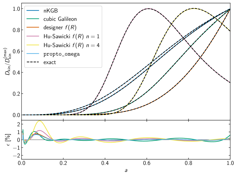
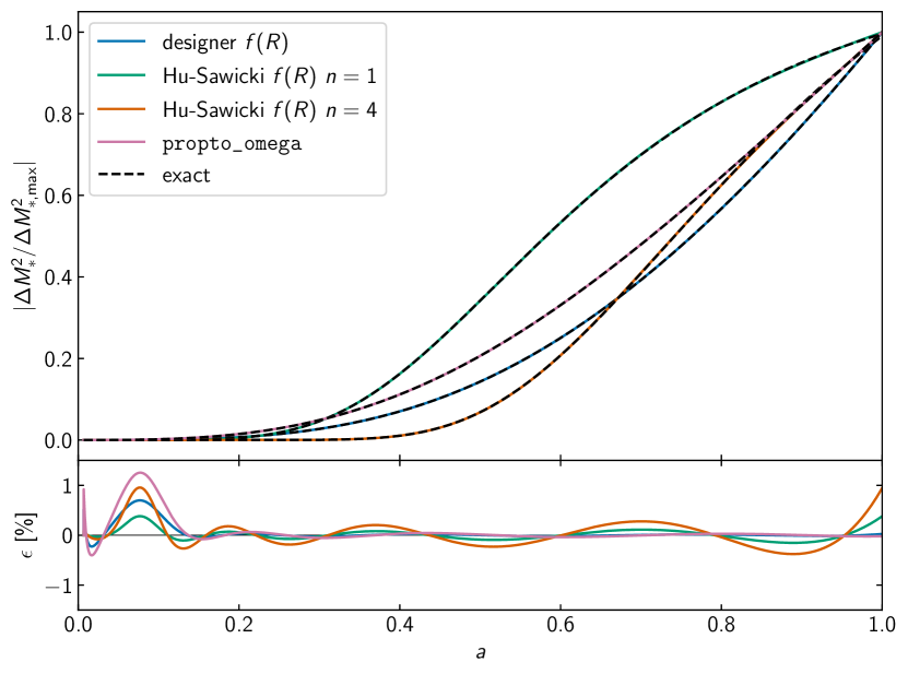
Figure 7: Reconstruction of the stable basis functions, with the left panel displaying the normalized de-mixed kinetic term ($D_{\text{kin}}/D_{\text{kin}}^{\rm(max)}$), and the right panel showing the normalized absolute deviations from the standard cosmological strength of gravity, $|\Delta M_{\ast}^{2}/\Delta M_{\ast,{\rm max}}^{2}|$. Coloured lines indicate the functions as reconstructed from the principal components and power-law approximation, while the dashed lines are the exact quantities. The lower sub-panels quantify the reconstruction accuracy, which is consistently better than 1% for the entire range where modified gravity significantly affect the growth of structure $a>0.1$.

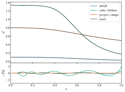
Figure 8: Reconstructed (coloured) and exact (dashed) speed of sound for the test models exhibiting non-trivial evolution (i.e., $c_{\rm s}^{2}\neq 1$). The lower panel demonstrates that the PCA-based reconstruction can achieve better than 1% accuracy at all times.

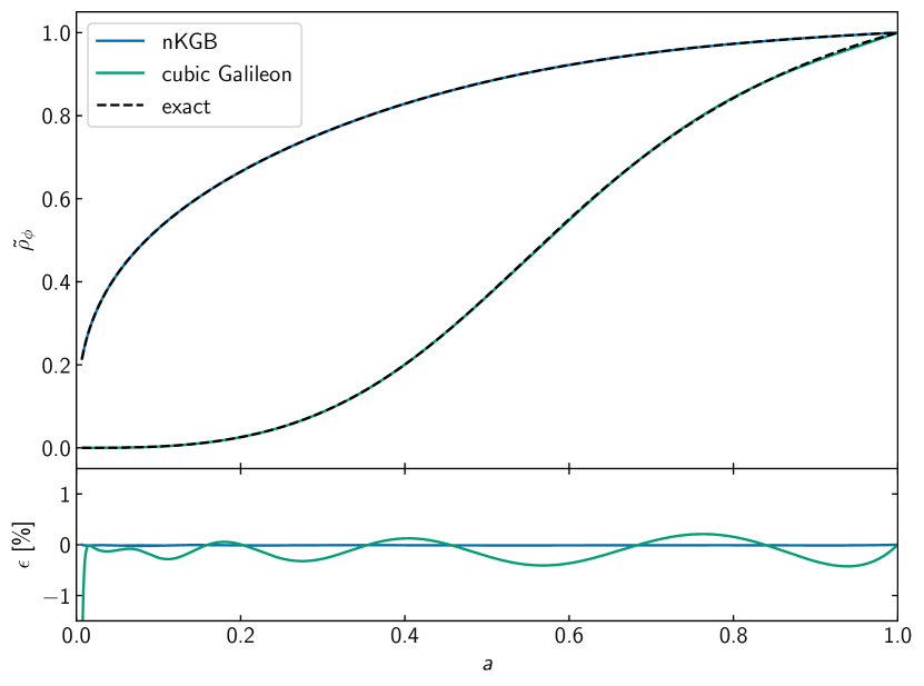
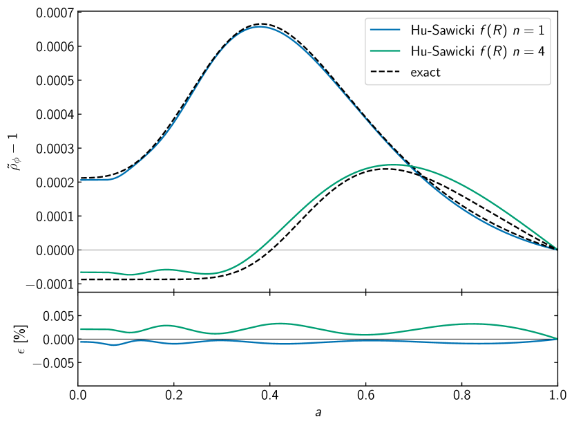
Figure 9: Comparison between the reconstructed background energy-density of the scalar field (coloured lines) and the exact calculations (dashed lines). The left panel shows the evolution of the energy-density for two models minimally coupled to gravity, whereas the right panel displays $\rho_{\phi}$ for two variants of the Hu-Sawicki (HS) $f(R)$ gravity model which feature a conformal coupling to gravity. For both types of models, the reconstructed quantities closely align with the exact references, maintaining the accuracy within 0.5% for scale factors $a>0.02$.

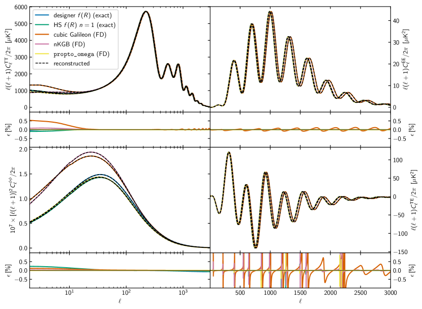
Figure 10: Comparison of the CMB auto- and cross-power spectra obtained with mochi_class using the reconstructed stable basis (dashed lines) against the exact predictions (coloured lines). For the cubic Galileon and nKGB models, as well as propto_omega, the reference spectra are generated by hi_class following the full scalar field dynamics (FD). The exact calculations for the two $f(R)$ gravity models are performed using mochi_class with the automatic method and precisely determined stable basis functions. For all reconstructed models, the initial conditions for the braiding parameter, $\alpha_{B0}$, are optimised to minimise the matter power spectrum’s relative deviation at $z=0$ compared to the exact models (refer to Equation 37). The small fractional differences, $\epsilon$, shown in the lower sub-panels indicate that the reconstructed models are observationally indistinguishable from their exact counterparts.

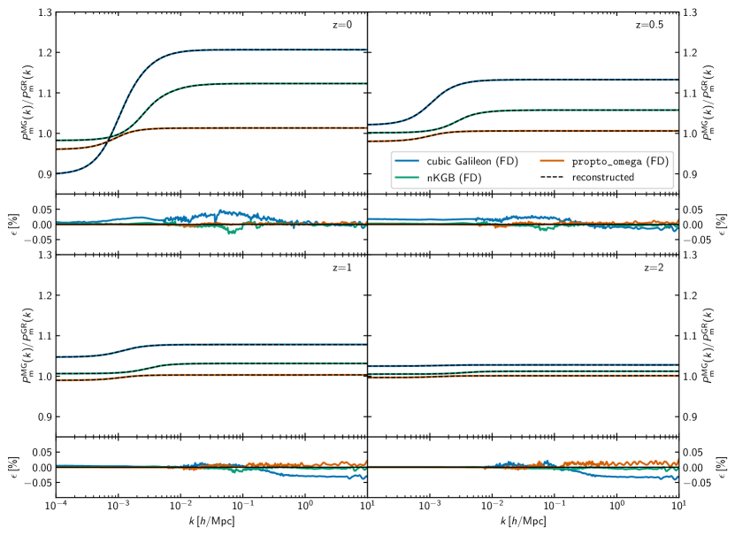
Figure 11: Evolution of the modified gravity-to-$\Lambda$CDM power spectrum ratio for three test models with scale-independent linear growth on sub-horizon scales. The colored lines represent the output from hi_class solving for the full dynamic (FD) of the scalar degree of freedom. The dashed lines are the mochi_class predictions for the reconstructed models, where the stable parameters, $\{\Delta M_{\ast}^{2},D_{\rm kin},c_{\rm s}^{2},\tilde{\rho}_{\phi}\}$, and the initial conditions, $\alpha_{B0}$, are computed as detailed in the main text. The excellent agreement between the exact and reconstructed power spectrum ratios, shown in the lower sub-panels, demonstrates that the combination of principal components with a power-law approximation successfully captures the linear growth of structure in these models.

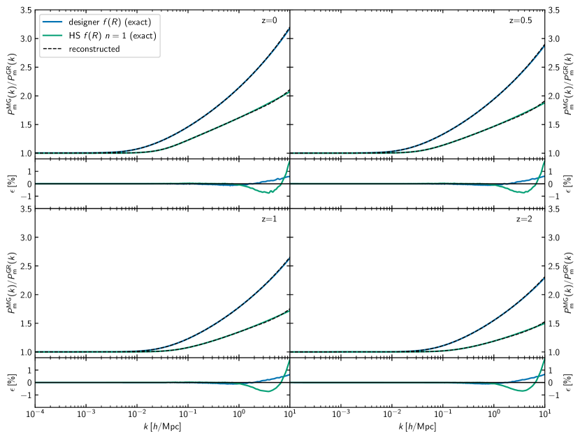
Figure 12: Evolution of the modified gravity-to-$\Lambda$CDM power spectrum ratio for two $f(R)$ gravity models–designer and Hu-Sawicki (HS). The colored lines represent the output from mochi_class using the exact input stable parameters, $\{\Delta M_{\ast}^{2},D_{\rm kin},c_{\rm s}^{2},\tilde{\rho}_{\phi}\}$, and initial conditions, $\alpha_{B0}$. The dashed lines are predictions from mochi_class using the reconstructed input functions, with initial conditions optimised to compensate for reconstruction inaccuracies. The lower sub-panels show that at all examined redshifts the reconstructed power spectra remain within 0.2% of the exact models for $k\lesssim 1\,h/{\rm Mpc}$, and within 1% for scales up to $k=8\,h/{\rm Mpc}$. However, reconstructing the HS model with $n=4$ (not shown) proved extremely difficult; despite sub-percent errors in the reconstructed stable functions (refer to Figs. 7 and 9), we could not determine initial conditions leading to stable perturbations.

Figures 7 to 9 illustrate the reconstruction accuracy of the principal components combined with the power law and/or constant approximation for the four basis functions in all of our test models. To project the exact functions onto the principal components, we first compute the natural logarithm of their absolute values . We then remove the power-law and/or constant trends from this quantity and finally apply the projection. For instance, to reconstruct the de-mixed kinetic term for any particular model, we do the following:

1. Compute the natural logarithm of the exact $D_{\rm kin}$.

2. Fit a power-law over the range $[-5,-3]$ to find the best fit parameters, $\zeta_{D}$ and $b_{D}$;

3. Subtract the power law from the exact $\ln(D_{\rm kin})$ to obtain $\Delta_{D}$;

4. Project $\Delta_{D}$ onto the six principal components to get $\tilde{\Delta}_{D}=\sum_{i}^{N_{D}}w_{i}\psi_{i}(x)$, where the $w_{i}$’s are the $N_{D}$ projection weights and $\psi_{i}$ is the $i$-th principal component.

5. Define the approximated function using Equation (33) by replacing $\Delta_{D}$ with $\tilde{\Delta}_{D}$.

From the lower panels of Figures 7-9 we observe that our PCA reconstruction matches the exact stable functions to within 1% for $a\gtrsim 0.05$. In a few cases, however, the relative difference, $\epsilon$, exhibits a peak exceeding the target accuracy around $a=0.1$. Due to negligible departures from $\Lambda$CDM at those redshifts, this is not concerning and has no measurable effect on the cosmological observables. For comparison, Figure 14 in Appendix B demonstrates that when using the same number of free parameters, alternative parametrisations of the $\Delta_{J}$ functions rooted in polynomial expansion underperform compared to the GP+PCA strategy adopted here.

To test how well the reconstructed stable functions describe the original MG cosmologies, we can use them as input to mochi_class to predict the background expansion and linear perturbations. To assess the performance of the background reconstruction, we examine the Hubble parameter and conclude that the reconstructed expansion history resembles the exact one to better than 0.2% for all models. However, having the full set of stable functions is not sufficient to compute the perturbations, as we also need the initial condition, $\alpha_{B0}$, for the integration of the braiding parameter. We determine this by minimizing the mean squared error

$${\rm MSE}[\alpha_{B0}]=\frac{1}{N_{k}}\sum_{k}\left[\frac{P_{\rm m}^{\rm rec.}(k|\alpha_{B0})}{P_{\rm m}^{\rm exact}(k)}-1\right]^{2}\,,$$ (37)

where $N_{k}$ is the total number of wavenumbers, $k$, in the interval $[10^{-4},10]\,h/{\rm Mpc}$, and $P_{\rm m}^{\rm rec.}(k|\alpha_{B0})$ and $P_{\rm m}^{\rm exact}(k)$ are the present-day matter power spectra of the reconstructed and exact model, respectively. The derived best-fit initial conditions are typically within 0.1-1% of their exact counterparts. Due to the high sensitivity of $f(R)$ gravity to small inaccuracies in the reconstructed functions (mainly $\Delta M_{\ast}^{2}$ and $\tilde{\rho}_{\phi}$), we could not find a satisfactory $\alpha_{B0}$ that produced stable perturbations for the Hu-Sawicki $n=4$ model. We do not reconstruct trivial stable functions: the speed of sound in $f(R)$ gravity is fixed at 1, $\Delta M_{\ast}^{2}=0$ for the cubic Galileon and nKGB models, and $\tilde{\rho}_{\phi}=1$ for propto_omega.

Figure 10 confirms that by combining GPs and PCA we can predict the secondary CMB anisotropies (i.e. lensing and ISW effect) sourced by the late-time modified growth of the test models to precision levels well within the expected uncertainties of CMB-S4 experiments (see, e.g., Ade et al., 2018). Matter power spectra for cubic Galileon, nKGB and propto_omega models are also reconstructed to $\lesssim 0.05\%$ precision across all redshifts, as shown in Figure 11. On the other hand, even though the reconstruction accuracy of the stable functions for $f(R)$ gravity never exceeds 1%, Figure 12 highlights that the derived matter power spectra deviate from the truth by $\lesssim 0.2\%$ only up to $k\approx 1\,h/{\rm Mpc}$, with the agreement degrading to 1% at $k\approx 8\,h/{\rm Mpc}$. Despite these relatively large differences on small scales, uncertainties in the non-linear evolution (Winther et al., 2015) and baryonic feedback (Chisari et al., 2019) have a much greater impact in this regime, effectively making the reconstructed models observationally indistiguishable from the true $f(R)$ gravity theories.

5.3 Exploring Horndeski’s landscape

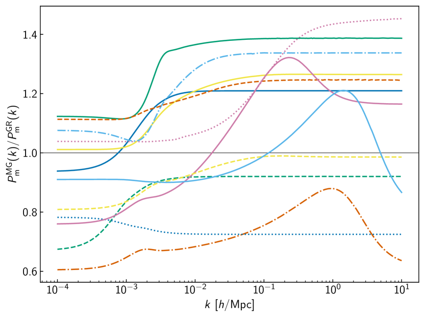
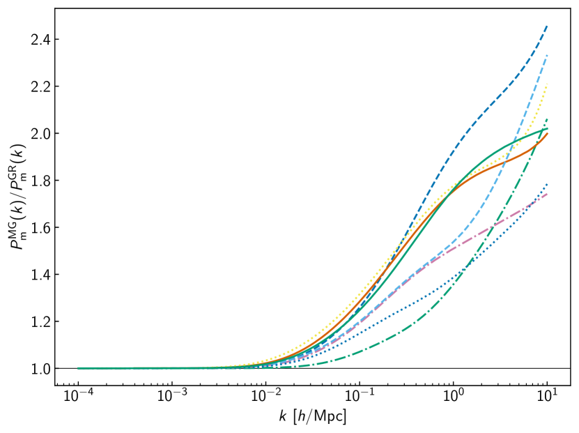
Figure 13: Ratios of the matter power spectrum at $z=0$ for randomly generated modified gravity models to that of $\Lambda$CDM. Left:: 12 stable models selected from a 31-dimensional parameter space, sampled via a Latin hypercube strategy. We use 6 principal components for each of the input functions, 2 power-law parameters to describe the early-time evolution of $\Delta M_{\ast}^{2}$, $D_{\rm kin}$ and $\tilde{\rho}_{\phi}$, as well as 1 scaling parameter setting the amplitude of $c_{\rm s}^{2}$ deep in the matter-dominated era. The initial conditions, $\alpha_{B0}$, are determined to ensure the solution to the braiding non-linear ODE (Equation 27) closely follows the expected behaviour at early times (Equation 5.3). The observed variety of power spectrum shapes demonstrates that the parametrisation of the stable functions proposed here can capture a richer phenomenology than the fixed-form parametrisations, like propto_omega, or traditional models, such as Galileons and nKGB. Right: 8 realisations drawn from a pool of stable models obtained by sampling a 16-dimensional parameter space with a Latin hypercube strategy. In this case we only parametrise $\Delta M_{\ast}^{2}$ and $\tilde{\rho}_{\phi}$ using 6 principal components and 2 power-law parameters. We set $c_{\rm s}^{2}=1$, and $D_{\rm kin}$ is given by $3\alpha_{\rm M}^{2}/2$. Initial conditions for the braiding follow the same methodology as the left panel. In this sub-space of the full Horndeski’s landscape, models with $\alpha_{\rm K}\ll\alpha_{\rm B}^{2}$ are closely related to $f(R)$ gravity theories. Indeed, the morphology of power spectrum ratios is similar yet more varied than the $f(R)$ gravity test models used in this work.

By combining mochi_class with the newly introduced parametrisation, Equation (33), we can venture beyond the phenomenological boundaries defined by the $\Lambda$CDM extensions discussed in Section 2. For this first exploratory task, we focus on two families of models:

1. Scalar Horndeski (SH): here, we exploit the full functional freedom provided by Equation (33) and use the GP+PCA basis presented in Section 5.1. For simplicity, we fix the number of principal components to six for all $\Delta_{J}$’s, and given the small contribution of the power-law term to the speed of sound (see Figure 8) we set $A_{c_{\rm s}}=0$. Therefore, we have a total of 31 parameters accounting for the power laws and PC weights.

2. $f(R)$-like (FR): this represents a particular sub-space of the SH cosmologies, where sampling can be extremely challenging without imposing specific relations for the stable functions. The freedom is limited to $\Delta M_{\ast}^{2}$ and $\tilde{\rho}_{\phi}$, with the remaining functions being $c_{\rm s}^{2}=1$ and $D_{\rm kin}=3\alpha_{\rm M}^{2}/2$. Models with $\alpha_{\rm K}\ll\alpha_{\rm B}^{2}$ closely resemble $f(R)$ gravity. To describe this sub-class we use six PC weights and two power-law parameters for each stable basis function.

In both cases we sample the parameter space using a Latin hypercube strategy with 5,000 sampling points for SH and 1,500 for FR. The parameters ranges defining the hypercube can be found in Appendix C.

As with the reconstruction of the test models, we need to choose a value for the initial condition, $\alpha_{B0}$. While in the former case we could use the exact calculations as reference and minimise Equation (37), here we are generating new models, and $\alpha_{B0}$ should be interpreted as an additional free parameter. However, if we want the early-time evolution of the braiding to be driven by the stable functions, we can impose an additional constraint to find suitable initial conditions. To see this, we start by linearising Equation (27) around $\alpha_{\rm B}=0$. This approximation is valid for times $x\leq x_{0}$, with $x_{0}$ sufficiently deep in the matter-dominated era, when we expect $\alpha_{\rm B}\rightarrow 0$. By applying the integrating factor technique, we can express the solution to the linearised non-homogeneous differential equation as

$$\alpha_{\rm B}^{\rm(lin)}(x)=\left[\mathcal{V}(x)+\alpha_{\rm B}(x_{0})\right]e^{\mathcal{G}(x)}\,,$$ (38)

where

$$e^{\mathcal{G}(x)}=\frac{H(x_{0})}{H(x)}\frac{M_{\ast}^{2}(x)}{M_{\ast}^{2}(x_{0})}e^{(x_{0}-x)}$$ (39)

represents the time-varying part of the homogeneous solution. The function $\mathcal{V}$ contributes to the particular solution that depends on the source term, $\mathcal{S}$. It is calculated by integrating the following differential equation with the associated initial condition:

$$\mathcal{V}^{\prime}=e^{-\mathcal{G}(x)}\mathcal{S}(x),\qquad\mathcal{V}(x_{0})=0\,.$$ (40)

Note that this equation contains no information about $\alpha_{B0}$. In contrast, $\alpha_{\rm B}(x_{0})$ does depend on the value of the braiding at $x=0$. In the regime of interest here, beside applying the approximations in Equation (34), we can also neglect radiation by setting $\Omega_{\rm r}=0$. This allows us to simplify the stable functions as power laws plus constants, write $(\nicefrac{{H}}{{H_{0}}})^{2}\approx\Omega_{\rm m}e^{-3x}$, and approximate $M_{\ast}^{2}(x)\approx M_{\ast}^{2}(x_{0})\approx 1$. Equation (40) can then be integrated analytically for all times $x\leq x_{0}$, and its solution consists of two parts: a constant term, $\bar{v}$, that depends on $x_{0}$, and a sum of power laws. In the limit $x\ll x_{0}$, the power laws vanish, leaving $\bar{v}$ as the only remaining contribution.

Now, let us assume a value $\alpha_{B0}$ such that $\alpha_{\rm B}(x_{0})$ is either larger or smaller than $-\bar{v}$. The early-time evolution of the approximate solution, Equation (38), will be controlled by the homogeneous solution, Equation (39), which ultimately scales as $\sim\pm\sqrt{e^{x}}$. This scaling is completely independent of the cosmological parameters and late-time dynamics defined by the stable functions. To avoid this spurious behaviour, we must adjust $\alpha_{B0}$ such that $\alpha_{B}(x_{0})=-\bar{v}$, which yields the following early-time solution:

$$\alpha_{\rm B}^{\rm(lin)}(x)\approx -\operatorname{sgn}(A_{M})\frac{2\zeta_{M}+3}{\zeta_{M}-1/2}e^{(\zeta_{M}x+b_{M})}$$

$$+\frac{C_{c_{\rm s}^{2}}}{\zeta_{D}-1/2}e^{(\zeta_{D}x+b_{D})}$$

$$+\operatorname{sgn}(A_{\rho})\left(\frac{1-\Omega_{\rm m}}{\Omega_{\rm m}}\right)\frac{\zeta_{\rho}}{\zeta_{\rho}+5/2}e^{(\zeta_{\rho}+3)x+b_{\rho}}\,.$$ (41)

As a case in point, we examine a designer $f(R)$ gravity cosmology with a $\Lambda$CDM background and $B_{0}\ll 1$. For this model, Equation (5.3) simplifies significantly, as we have $c_{\rm s}^{2}=1$, $D_{\rm kin}=3\alpha_{\rm M}^{2}/2\ll\alpha_{\rm M}$, and $\tilde{\rho}_{\phi}=1$. From the definition of the running, Equation (3), and by imposing the condition $\alpha_{\rm B}=-\alpha_{\rm M}$, we derive a quadratic equation for the slope of $\Delta M_{\ast}^{2}$, with the positive solution being $\zeta_{M}=(5+\sqrt{73})/4$. Reassuringly, this result matches the value derived by Pogosian & Silvestri (2007) in the limit $\Omega_{\rm r}\rightarrow 0$ (see also Lombriser et al., 2018).

Finally, for each set of principal component weights, constants, power-law slopes, and amplitudes, we compute the stable functions and use Equation (5.3) as an early-time target for the integrated braiding solution to obtain $\alpha_{B0}$. In practice, we find the zero of the function defined as the definite integral over the range $x\in[-5,-4]$ of the difference $\alpha_{\rm B}^{\rm(ode)}-\alpha_{\rm B}^{\rm(lin)}$, where $\alpha_{\rm B}^{\rm(ode)}$ is the solution to Equation (27). For this step, we run only the background module of mochi_class and search for $\alpha_{B0}$ in the interval $[0,2]$ . The root finder typically takes 6-7 iterations to reach convergence. Consequently, this process slightly degrades the performance presented in Section 4.3 since more time must be spent on the background calculations.

The left panel of Figure 13 shows the present-day matter power spectrum ratio for 12 models selected from approximately 200 stable cosmologies generated using the SH Latin hypercube. A viability rate of 4% might seem surprising given that all 5,000 sample models pass the stability criteria, Equation (22). However, only a small fraction of these models feature stable perturbations not affected by exponentially growing modes, highlighting the importance of starting from the stable basis functions–using the $\alpha_{i}$’s to sample this parameter space would be even more challenging. Similar arguments apply to the right panel, where we find a higher stability rate of 20%, owing to the considerably smaller parameter volume.

Returning to the left panel, the variety of shapes for the matter power spectrum ratios reflects the rich phenomenology of the SH landscape. Besides the familiar behavior displayed by models such as cubic Galileon, nKGB, and propto_omega, the growth of structure can be slower than in $\Lambda$CDM, and can also exhibit non-trivial scale dependence arising from the interplay between the braiding scale, the Compton scale, and the scalar field sound horizon (see, e.g., Sawicki et al., 2012; Bellini & Sawicki, 2014, for detailed discussions).

As expected, the power spectrum ratios shown in the right panel of Figure 13 generally follow the trend of our test $f(R)$ cosmologies (see, e.g., Figure 4). However, the particular scale dependence can depart significantly from the commonly adopted designer and Hu-Sawicki models. This behaviour can be primarily attributed to (i) a different, possibly time-dependent, gravitational coupling in the sub-Compton limit (i.e., $\mu_{\infty}\neq\mu_{\infty}^{f(R)}=4/3$), and (ii) a more complex evolution of the Compton wavelength.

6 Summary and outlook

Horndeski gravity provides a comprehensive theoretical framework to explore scalar-tensor extensions of GR, offering rich phenomenology through diverse background expansion and structure formation scenarios. To study this extensive Horndeski landscape, we can restrict ourselves to the energy scales relevant to cosmology by adopting an effective-theory approach. In this work, we have introduced a numerical tool to facilitate the study and statistical analysis of Horndeski models expressed in the effective-theory language.

At the level of the background and linear perturbations, models within the scalar Horndeski sub-class are entirely described by four functions of time. The common $\alpha$-parametrisation, proposed by Bellini & Sawicki (2014), neatly separates the phenomenology of the background from that of the growth of structure and is implemented in Einstein-Boltzmann solver hi_class. This code also includes the quasi-static approximation scheme for improved computational efficiency and to extend applicability to models where following the full dynamics of the scalar field is challenging.

Despite these key computational advances, to reliably extend the use of hi_class to a broader portion of the Horndeski landscape, we must first address the following critical points:

• Simplify the implementation of specific models, which currently still requires modifications to the source code.

• Generalise the input functions to more flexible parametrisations, going beyond $\{w_{0},w_{a}\}$ for $\rho_{\phi}$, and $\propto\Omega_{\phi}(a)$ or $a^{s}$ for the $\alpha$-functions.

• Efficiently select stable models, eliminating the need to search for parameter combinations free from ghost and gradient instabilities.

• Improve on the accuracy of the QSA implementation in hi_class.

• Correct the erroneous labeling of healthy models as unstable due to limited numerical precision in the calculation of $c_{\rm s}^{2}$.

The hi_class extension released with this work, mochi_class, effectively resolves all the points above by:

• Replacing the $\alpha$-functions directly with the parameters used in the stability conditions, $\{D_{\rm kin},M_{\ast}^{2},c_{\rm s}^{2}\}$. To ensure the absence of ghosts and gradient instabilities, users need only to provide positive input functions.

• Accepting general functions of time as input, with the constraints $c_{\rm sN}^{2}\rightarrow 0$, $M_{\ast}^{2}\rightarrow 1$, and $\rho_{\phi}\ll\rho_{\rm m}$ deep in the matter-dominated era. In other words, the model must resemble the $\Lambda$CDM cosmology at early times.

• Including mathematical (or classical) stability conditions to catch exponentially growing modes, as done in EFTCAMB.

• Embedding a QSA implementation based on modified Poisson-like equations for the metric potentials.

We validated mochi_class’s accuracy and performance by comparing its output power spectra and computational efficiency to those of the publicly available Einstein-Boltzmann solvers hi_class, EFTCAMB, and MGCAMB. For all tested cases, we found that the predicted changes to the CMB spectra due to new physics matched the output from the other solvers within 0.05%, while for the matter power spectrum, the agreement reached 0.01%. Thanks to its alternative QSA implementation and to the manifestly stable EFT basis, mochi_class generally improves on the accuracy and numerical stability attained by hi_class, with $f(R)$ gravity being an extreme case that hi_class cannot even solve.

In addition, we proposed a new parametrisation for the stable functions and the background energy-density of the scalar field. This approach uses a simple early-time power-law (or constant) evolution and models late-time smooth deviations with Gaussian Processes, combined with principal component analysis for dimensionality reduction. We showed that this parametrisation can accurately reconstruct our test cosmologies, both in terms of input functions and output power spectra. As an initial application, we used it to generate Horndeski models with either all input functions free or by fixing relations and values to closely resemble $f(R)$ gravity. The linear growth of structure in these models can vary significantly, deviating from the well-known behavior of our test models. This diversity emphasises the necessity of exploring beyond the commonly employed parametrisations (see also Raveri et al., 2021, for a discussion on biased constraints and information loss).

The high versatility of class’s Python wrapper, classy, ensures mochi_class seamless integration into the pipeline of cosmological analyses using data probing both the background evolution and the linear regime of structure formation. This will provide an alternative avenue of investigation to the reconstruction strategies employed in, e.g., Raveri (2019); Zucca et al. (2019a) and Pogosian et al. (2021); Raveri et al. (2021), and will extend the analysis of studies based on fixed-form parametrisations of the $\alpha$- or EFT-functions (e.g., Salvatelli et al., 2016; Noller & Nicola, 2018; Aghanim et al., 2018; Seraille et al., 2024). In a future release, we will also include a special case of the stable parametrisation enforcing the relation $\alpha_{\rm B}=b\alpha_{\rm M}$, which can be more effective for analyses restricted to models in the generalised Brans-Dicke sub-class (Bergmann, 1968), where $\alpha_{\rm B}=-\alpha_{\rm M}$, or to investigate no-slip gravity modifications (Linder, 2018), defined by $\alpha_{\rm B}=-2\alpha_{\rm M}$.

The larger volume of Horndeski theory space covered by the new parametrisation will likely require scalable sampling methods capable of efficiently handling the high dimensionality of the problem (Mootoovaloo et al., 2024). One such method is Hamiltonian Monte Carlo (e.g., Hajian, 2006), a gradient-based sampling technique that leverages the derivatives of the likelihood function to significantly enhance the acceptance rate of samples in high-dimensional spaces. To implement this, we could rewrite mochi_class using the JAX framework, taking advantage of its automatic differentiation capabilities, as demonstrated by Hahn et al. (2023). Alternatively, a simpler approach might involve using mochi_class to generate training data for neural network emulators targeted to specific summary statistics (Mancini et al., 2021; Bonici et al., 2023). These emulators can then be integrated into cosmology libraries that feature automatic differentiation (Piras & Mancini, 2023; Campagne et al., 2023).

Finally, for general Horndeski models, mochi_class’s calculations represent a fundamental first step towards accessing the cosmological information contained on small scales (Heymans & Zhao, 2018). For instance, in the halo model reaction framework (Cataneo et al., 2018; Giblin et al., 2019), the linear matter power spectrum and background evolution are key ingredients for obtaining the mean halo statistics and non-linear matter power spectrum of non-standard cosmologies. This method, implemented in the ReACT code (Bose et al., 2020), can be applied to Lagrangian-based theories of gravity (Cataneo et al., 2018; Bose et al., 2021; Atayde et al., 2024; Bose et al., 2024), to phenomenological modifications to GR (Srinivasan et al., 2021, 2023), to an interacting dark sector (Carrilho et al., 2021), and to a broader class of parametrised $\Lambda$CDM extensions within the Horndeski realm (Bose et al., 2022).

Appendix A Precision parameters used in class and CAMB

The level of agreement between class and CAMB strongly depends on the precision settings adopted in the two codes (Lesgourgues, 2011b). To minimize the impact of numerical errors on the power spectra produced by different implementation strategies, code comparison analyses often employ high-precision settings (Bellini et al., 2017). Following this philosophy, we use high-precision parameter values for both mochi_class and hi_class,

    start_small_k_at_tau_c_over_tau_h = 1e-4
    start_large_k_at_tau_h_over_tau_k = 1e-4
    perturbations_sampling_stepsize = 0.01
    l_logstep = 1.026
    l_linstep = 25
    k_max_tau0_over_l_max = 8.
    k_per_decade_for_pk = 200
    l_max_scalars = 5000
    P_k_max_h/Mpc = 12.
    delta_l_max = 1000
    l_switch_limber = 50

Similarly for MGCAMB and EFTCAMB we use

    get_transfer = T
    transfer_high_precision = T
    high_accuracy_default = T
    k_eta_max_scalar = 80000
    do_late_rad_truncation = F
    accuracy_boost = 2
    l_accuracy_boost = 2
    l_sample_boost = 2
    l_max_scalar = 10000
    accurate_polarization = T
    accurate_reionization = T
    lensing_method =1
    use_spline_template = T

In addition, for EFTCAMB we set

    EFTCAMB_turn_on_time = 1e-10
    EFTtoGR = 1e-10

and for MGCAMB we use the default

    GRtrans = 1e-3

Appendix B Reconstruction with Padé approximants

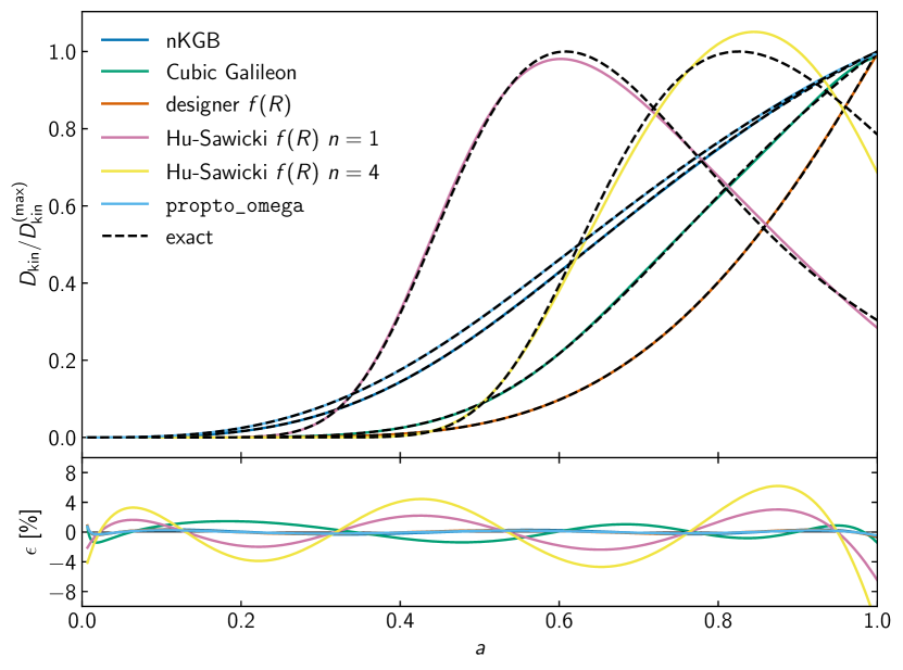
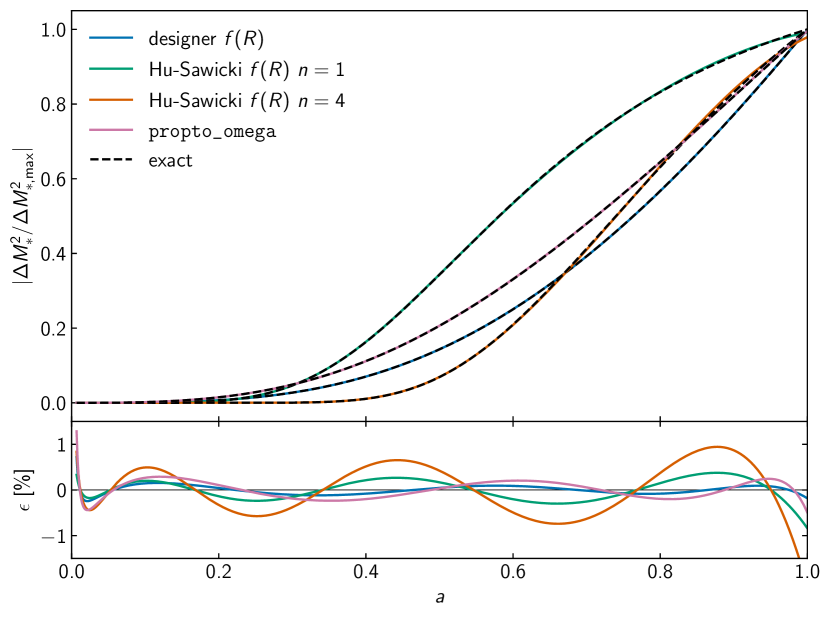
Figure 14: Reconstruction of two stable basis functions using Padé approximants (Equation 42). The left panel illustrates the normalized de-mixed kinetic term ($D_{\text{kin}}/D_{\text{kin}}^{\text{(max)}}$), while the right panel displays the normalized absolute deviations from the standard cosmological strength of gravity ($|\Delta M^{2}/\Delta M^{2}_{\ast,\text{max}}|$). The coloured lines represent functions reconstructed by fitting Padé approximants to their exact counterparts (dashed lines), once the early-time power-law trend has been subtracted. We maintain an identical number of free parameters as in the PCA-based approach to ensure a fair comparison. The lower sub-panels show the reconstruction accuracy of the fittings, indicating that the Padé approximants result in larger deviations from the exact models compared to the PCA-based reconstructions.

A Padé approximant of order $[N/M]$ for a function $f(x)$ is given by the ratio of two polynomials of degrees $N$ and $M$,

$$Q(x)=\frac{\sum_{n=0}^{N}\alpha_{n}\left(x-x_{0}\right)^{n}}{1+\sum_{m=1}^{M}\beta_{m}\left(x-x_{0}\right)^{m}}\;,$$ (42)

where the coefficients $\alpha_{n}$ and $\beta_{m}$ are chosen such that the Taylor series expansion of $Q(x)$ around $x=x_{0}$ matches the Taylor expansion of $f(x)$ up to order $N+M$.

Here, we quantify the reconstruction accuracy of the Padé approximants for the deviations, $\Delta_{J}$, used in the new parametrisation of the stable functions described in Section 5. We perform the expansions around $x_{0}=0$, but have verified that our conclusions are not sensitive to this particular choice. Since we lack analytical expressions for the $\Delta_{J}$ of our test models, we cannot derive the Padé coefficients by matching the Taylor series of $\Delta_{J}$ order by order. Instead, we interpret Equation (42) as a fitting function and determine the best-fit values for $\alpha_{n}$ and $\beta_{m}$ by minimising the reconstruction error. To ensure a fair comparison with the GP + PCA strategy discussed in Section 5.1, we use the same number of free parameters by setting $N=2$ and $M=3$, except for $\Delta_{M}$, where $N=3$.

Figure 14 illustrates the performance of the Padé approximants for two representative cases: $D_{\rm kin}$ and $\Delta M_{\ast}^{2}$. Reconstruction errors can reach approximately 8% for the de-mixed kinetic term and around 1% for the Planck mass shift. In comparison, Figure 7 demonstrates that our GP + PCA approach can match the exact quantities to better than 1%, which motivates the use of this reconstruction technique.

Appendix C Latin hypercube boundaries

Table 3 and 4 list the parameter ranges defining the Latin hypercubes used to generate random models belonging to the Scalar Horndeski and $f(R)$-like classes, respectively (see Section 5.3).

	$\zeta_{J}$	$b_{J}$	$C_{J}$	$w_{1}$	$w_{2}$	$w_{3}$	$w_{4}$	$w_{5}$	$w_{6}$
$\Delta M_{\ast}^{2}$	$[2,15]$	$[-6,3]$	–	$[0,250]$	$[0,150]$	$[0,50]$	$[0,10]$	$[0,5]$	$[-1,0]$
$D_{\rm kin}$	$[2,20]$	$[-5,5]$	–	$[-35,0]$	$[-50,0]$	$[0,5]$	$[0,5]$	$[-2,2]$	$[-1,1]$
$c_{\rm s}^{2}$	undefined	$-\infty$	$[0,2]$	$[0,30]$	$[-30,0]$	$[-15,0]$	$[0,3]$	$[-1,1]$	$[-1,1]$
$\tilde{\rho}_{\phi}$	$[-1,3]$	$[-2,2]$	derived	$[-10,10]$	$[-8,8]$	$[-4,4]$	$[-1,1]$	$[-1,1]$	$[-1,1]$

Table 3: Parameter ranges used to generate the 5,000 Scalar Horndeski sample models following the parametrisation in Equation (33) combined with the PCA basis functions described in Section 5.1. We fix $\operatorname{sgn}(A_{M})=-1$ and $\operatorname{sgn}(A_{\rho})=+1$.

	$\zeta_{J}$	$b_{J}$	$C_{J}$	$w_{1}$	$w_{2}$	$w_{3}$	$w_{4}$	$w_{5}$	$w_{6}$
$\Delta M_{\ast}^{2}$	$[4,15]$	$[-6,-2]$	–	$[0,250]$	$[0,50]$	$[0,10]$	$[0,5]$	$[0,5]$	$[-1,0]$
$\tilde{\rho}_{\phi}$	0	$[-0.1,0.1]$	derived	$[-1,1]\cdot 10^{-3}$	$[-1,1]\cdot 10^{-3}$	$[-5,5]\cdot 10^{-4}$	$[-1,1]\cdot 10^{-4}$	$[-1,1]\cdot 10^{-4}$	$[-1,1]\cdot 10^{-4}$

Table 4: Parameter ranges used to generate the 1,500 $f(R)$-like sample models following the parametrisation in Equation (33) combined with the PCA basis functions described in Section 5.1. We fix $\operatorname{sgn}(A_{M})=-1$ and $\operatorname{sgn}(A_{\rho})=+1$.

Appendix D Useful equations in mochi_class

D.1 Continuity equation

When users select expansion_model = wext, the scalar field background energy-density, $\rho_{\phi}$, is integrated using the following continuity equation with the corresponding initial condition:

$$\dot{\rho}_{\phi}=-3\rho_{\phi}(1+w_{\phi})\,,\qquad\rho_{\phi}(0)=\Omega_{\phi}H_{0}^{2}\,.$$ (43)

Here we remind the reader that overdots denote derivatives with respect to $\ln a$, and primes (used below) represent derivatives with respect to conformal time. The choice between $\ln a$ or $\tau$ as the time variable is dictated by the original class structure, with the former used in the background module and the latter in the perturbations module.

D.2 Scalar field fluctuations

The coefficients and the source term in Equation (23) can be found in Appendix A.2 of  Zumalacarregui et al. (2016). For convenience, we provide them here:

$$\mathcal{A}(\tau)=D_{\rm kin}(2-\alpha_{\rm B})\,,$$ (44a)

$$\mathcal{B}(\tau)=8aH\lambda_{7}\,,$$ (44b)

$$\mathcal{C}(\tau)=-8a^{2}H^{2}\lambda_{8}\,,$$ (44c)

$$\mathcal{D}(\tau)=2c_{\rm sN}^{2}\,,$$ (44d)

$$\mathcal{E}(\tau,k)=\frac{2c_{\rm sN}^{2}}{aH}k^{2}\eta+\frac{3a}{2HM_{\ast}^{2}}\left[2\lambda_{2}\delta\rho_{\rm m}-3\alpha_{\rm B}(2-\alpha_{\rm B})\delta p_{\rm m}\right]\,,$$ (44e)

where

$$\lambda_{2}=-\frac{3(\rho_{\rm m}+p_{\rm m})}{H^{2}M_{\ast}^{2}}-(2-\alpha_{\rm B})\frac{H^{\prime}}{aH^{2}}+\frac{\alpha_{\rm B}^{\prime}}{aH}\,,$$ (45a)

$$\lambda_{7}=\frac{D_{\rm kin}}{8}(2-\alpha_{\rm B})\left[4+\alpha_{\rm M}+\frac{2H^{\prime}}{aH^{2}}+\frac{D_{\rm kin}^{\prime}}{aHD_{\rm kin}}\right]+\frac{D_{\rm kin}}{8}\lambda_{2}\,,$$ (45b)

$$\lambda_{8}=-\frac{\lambda_{2}}{8}(D_{\rm kin}-3\lambda_{2}+\frac{3\alpha_{\rm B}^{\prime}}{aH})+\frac{1}{8}(2-\alpha_{\rm B})\left[(3\lambda_{2}-D_{\rm kin})\frac{H^{\prime}}{aH^{2}}-\frac{9\alpha_{\rm B}p_{\rm m}^{\prime}}{2aH^{3}M_{\ast}^{2}}\right]$$

$$\quad\quad\,-\frac{D_{\rm kin}}{8}(2-\alpha_{\rm B})\left[4+\alpha_{\rm M}+\frac{2H^{\prime}}{aH^{2}}+\frac{D_{\rm kin}^{\prime}}{aHD_{\rm kin}}\right]\,.$$ (45c)

D.3 Quasi-static approximation

In the effective-field formulation of the quasi-static approximation, the gravitational coupling for the non-relativistic matter and the gravitational slip can be expressed as in Equation (31). The small-scale limits can be expressed in terms of the $\alpha$’s as

$$\mu_{\infty}=\frac{2c_{\rm sN}^{2}+(\alpha_{\rm B}+2\alpha_{\rm M})^{2}}{2c_{\rm sN}^{2}M_{\ast}^{2}}\,,\qquad\mu_{Z,\infty}=\frac{2c_{\rm sN}^{2}+\alpha_{\rm B}(\alpha_{\rm B}+2\alpha_{\rm M})}{2c_{\rm sN}^{2}M_{\ast}^{2}}\,,$$ (46)

while

$$\mu_{\rm p}=\frac{9\left\{aH\left[2c_{\rm sN}^{2}+(\alpha_{\rm B}-2)\alpha_{\rm B}+4(\alpha_{\rm B}-1)\alpha_{\rm M}\right](\rho_{\rm m}+p_{\rm m}+\rho_{\phi}+p_{\phi})+2\alpha_{\rm B}(p_{\rm m}^{\prime}+p_{\phi}^{\prime})\right\}}{4aH^{3}}\,.$$ (47)

Here, we also present a typo-corrected equation for the metric perturbations in synchronous gauge, $\eta$, used in our MGCAMB patch to hi_class:

$$\eta^{\prime} =\frac{1}{2}\frac{a^{2}}{9\rho_{\rm m}a^{2}\mu\gamma(1+w_{\rm m})/2+k^{2}}\left\{3\rho_{\rm m}(1+w_{\rm m})\mu\gamma\theta\left[1+3\left(\frac{{\mathcal{H}}^{2}-{\mathcal{H}}^{\prime}}{k^{2}}\right)\right]+3\rho_{\rm m}\Delta_{\rm m}\left[{\mathcal{H}}\mu(\gamma-1)-\mu^{\prime}\gamma-\mu^{\prime}{\gamma}\right]\right.$$

$$+9\mu(1-\gamma)\rho_{\rm m}(1+w_{\rm m})\sigma_{\rm m}^{\prime}+k^{2}\alpha\left[3\rho_{\rm m}\mu\gamma(1+w_{\rm m})-2\left(\frac{\mathcal{H}^{2}-\mathcal{H}^{\prime}}{a^{2}}\right)\right]+9{\mathcal{H}}\mu(\gamma-1)(1+w_{\rm m})\rho_{\rm m}\sigma_{\rm m}(3w_{\rm m}+2)$$

$$\left.-9(1+w_{\rm m})\rho_{\rm m}\sigma_{\rm m}\left[\mu^{\prime}(\gamma-1)+\gamma^{\prime}\mu+\mu(\gamma-1)\frac{w_{\rm m}^{\prime}}{1+w_{\rm m}}\right]\right\}\,,$$ (48)

where $\mathcal{H}$ is the conformal Hubble parameter. The corrections compared to Equation (26) in Zucca et al. (2019b) include removing an extra power of two from $\mathcal{H^{\prime}}$ in the first line, and changing the minus sign to a plus sign in front of the $\gamma^{\prime}\mu$ term in the last line.

References

- Abdalla et al. (2022) Abdalla, E., Abellán, G. F., Aboubrahim, A., et al. 2022, Journal of High Energy Astrophysics, 34, 49, doi: 10.1016/j.jheap.2022.04.002
- Ade et al. (2018) Ade, P., Aguirre, J., Ahmed, Z., et al. 2018, Journal of Cosmology and Astroparticle Physics, 2019, doi: 10.1088/1475-7516/2019/02/056
- Aghanim et al. (2018) Aghanim, N., Akrami, Y., Ashdown, M., et al. 2018, Astronomy and Astrophysics, 641, doi: 10.1051/0004-6361/201833910
- Aigrain & Foreman-Mackey (2022) Aigrain, S., & Foreman-Mackey, D. 2022, Annual Review of Astronomy and Astrophysics, 61, 329, doi: 10.1146/annurev-astro-052920-103508
- Atayde et al. (2024) Atayde, L., Frusciante, N., Bose, B., Casas, S., & Li, B. 2024. https://arxiv.org/abs/2404.11471v1
- Aviles & Cervantes-Cota (2017) Aviles, A., & Cervantes-Cota, J. L. 2017, Physical Review D, 96, doi: 10.1103/PhysRevD.96.123526
- Baker et al. (2017) Baker, T., Bellini, E., Ferreira, P. G., et al. 2017, Physical Review Letters, 119, doi: 10.1103/PhysRevLett.119.251301
- Bellini et al. (2015) Bellini, E., Cuesta, A. J., Jimenez, R., & Verde, L. 2015, Journal of Cosmology and Astroparticle Physics, 2016, doi: 10.1088/1475-7516/2016/02/053
- Bellini & Sawicki (2014) Bellini, E., & Sawicki, I. 2014, Journal of Cosmology and Astroparticle Physics, 2014, doi: 10.1088/1475-7516/2014/07/050
- Bellini et al. (2019) Bellini, E., Sawicki, I., & Zumalacárregui, M. 2019, Journal of Cosmology and Astroparticle Physics, 2020, doi: 10.1088/1475-7516/2020/02/008
- Bellini et al. (2017) Bellini, E., Barreira, A., Frusciante, N., et al. 2017, Physical Review D, 97, doi: 10.1103/PhysRevD.97.023520
- Bergmann (1968) Bergmann, P. G. 1968, International Journal of Theoretical Physics 1968 1:1, 1, 25, doi: 10.1007/BF00668828
- Blas et al. (2011) Blas, D., Lesgourgues, J., & Tram, T. 2011, Journal of Cosmology and Astroparticle Physics, 2011, doi: 10.1088/1475-7516/2011/07/034
- Bloomfield et al. (2012) Bloomfield, J. K., Éanna É. Flanagan, Park, M., & Watson, S. 2012, Journal of Cosmology and Astroparticle Physics, 2013, doi: 10.1088/1475-7516/2013/08/010
- Bonici et al. (2023) Bonici, M., Bianchini, F., & Ruiz-Zapatero, J. 2023, Open Journal of Astrophysics, 7, doi: 10.21105/astro.2307.14339
- Bose et al. (2020) Bose, B., Cataneo, M., Tröster, T., et al. 2020, Monthly Notices of the Royal Astronomical Society, 498, 4650, doi: 10.1093/mnras/staa2696
- Bose & Koyama (2016) Bose, B., & Koyama, K. 2016, Journal of Cosmology and Astroparticle Physics, 2016, doi: 10.1088/1475-7516/2016/08/032
- Bose et al. (2022) Bose, B., Tsedrik, M., Kennedy, J., et al. 2022, Monthly Notices of the Royal Astronomical Society, 519, 4780, doi: 10.1093/mnras/stac3783
- Bose et al. (2021) Bose, B., Wright, B. S., Cataneo, M., et al. 2021, Monthly Notices of the Royal Astronomical Society, 508, 2479, doi: 10.1093/mnras/stab2731
- Bose et al. (2024) Bose, B., Gupta, A. S., Fiorini, B., et al. 2024. https://arxiv.org/abs/2406.13667v1
- Campagne et al. (2023) Campagne, J.-E., Lanusse, F., Zuntz, J., et al. 2023, Open Journal of Astrophysics, 6, doi: 10.21105/astro.2302.05163
- Carrilho et al. (2021) Carrilho, P., Carrion, K., Bose, B., et al. 2021, Monthly Notices of the Royal Astronomical Society, 512, 3691, doi: 10.1093/mnras/stac641
- Castello et al. (2024) Castello, S., Mancarella, M., Grimm, N., et al. 2024, JCAP, 05, 003, doi: 10.1088/1475-7516/2024/05/003
- Cataneo et al. (2018) Cataneo, M., Lombriser, L., Heymans, C., et al. 2018, Monthly Notices of the Royal Astronomical Society, 488, 2121, doi: 10.1093/mnras/stz1836
- Chisari et al. (2019) Chisari, N. E., Mead, A. J., Joudaki, S., et al. 2019, The Open Journal of Astrophysics, 2, doi: 10.21105/astro.1905.06082
- Chudaykin & Kunz (2024) Chudaykin, A., & Kunz, M. 2024. https://arxiv.org/abs/2407.02558v1
- Clifton et al. (2011) Clifton, T., Ferreira, P. G., Padilla, A., & Skordis, C. 2011, Physics Reports, 513, 1, doi: 10.1016/j.physrep.2012.01.001
- Collaboration et al. (2017) Collaboration, L. S., Collaboration, V., Monitor, F. G.-R. B., & INTEGRAL. 2017, The Astrophysical Journal Letters, 848, L13, doi: 10.3847/2041-8213/aa920c
- Copeland et al. (2006) Copeland, E. J., Sami, M., & Tsujikawa, S. 2006, International Journal of Modern Physics D, 15, 1753, doi: 10.1142/S021827180600942X
- Creminelli & Vernizzi (2017) Creminelli, P., & Vernizzi, F. 2017, Physical Review Letters, 119, doi: 10.1103/PhysRevLett.119.251302
- Cusin et al. (2017) Cusin, G., Lewandowski, M., & Vernizzi, F. 2017, Journal of Cosmology and Astroparticle Physics, 2018, doi: 10.1088/1475-7516/2018/04/005
- de Rham & Melville (2018) de Rham, C., & Melville, S. 2018, Physical Review Letters, 121, doi: 10.1103/PhysRevLett.121.221101
- Deffayet et al. (2009a) Deffayet, C., Deser, S., & Esposito-Farèse, G. 2009a, Phys.Rev.D, 80, doi: 10.1103/PHYSREVD.80.064015
- Deffayet et al. (2009b) Deffayet, C., Esposito-Farese, G., & Vikman, A. 2009b, Physical Review D - Particles, Fields, Gravitation and Cosmology, 79, doi: 10.1103/PhysRevD.79.084003
- Deffayet et al. (2010) Deffayet, C., Pujolas, O., Sawicki, I., & Vikman, A. 2010, Journal of Cosmology and Astroparticle Physics, 2010, doi: 10.1088/1475-7516/2010/10/026
- Denissenya & Linder (2018) Denissenya, M., & Linder, E. V. 2018, Journal of Cosmology and Astroparticle Physics, 2018, doi: 10.1088/1475-7516/2018/11/010
- DES Collaboration et al. (2021) DES Collaboration, Abbott, T. M. C., Aguena, M., et al. 2021, Physical Review D, 105, 30, doi: 10.1103/PhysRevD.105.023520
- eBOSS Collaboration et al. (2020) eBOSS Collaboration, Alam, S., Aubert, M., et al. 2020, Physical Review D, 103, 17, doi: 10.1103/PhysRevD.103.083533
- Ezquiaga & Zumalacárregui (2017) Ezquiaga, J. M., & Zumalacárregui, M. 2017, Physical Review Letters, 119, doi: 10.1103/PhysRevLett.119.251304
- Ezquiaga & Zumalacárregui (2018) —. 2018, Frontiers in Astronomy and Space Sciences, 5, doi: 10.3389/fspas.2018.00044
- Felice & Tsujikawa (2010a) Felice, A. D., & Tsujikawa, S. 2010a, Physical Review Letters, 105, doi: 10.1103/PhysRevLett.105.111301
- Felice & Tsujikawa (2010b) —. 2010b, Living Reviews in Relativity, 13, doi: 10.12942/lrr-2010-3
- Frusciante et al. (2018) Frusciante, N., Papadomanolakis, G., Peirone, S., & Silvestri, A. 2018, Journal of Cosmology and Astroparticle Physics, 2019, doi: 10.1088/1475-7516/2019/02/029
- Giblin et al. (2019) Giblin, B., Cataneo, M., Moews, B., & Heymans, C. 2019, Monthly Notices of the Royal Astronomical Society, 490, 4826, doi: 10.1093/mnras/stz2659
- Gleyzes (2017) Gleyzes, J. 2017, Physical Review D, 96, doi: 10.1103/PhysRevD.96.063516
- Gsponer & Noller (2021) Gsponer, R., & Noller, J. 2021, Physical Review D, 105, doi: 10.1103/PhysRevD.105.064002
- Hahn et al. (2023) Hahn, O., List, F., & Porqueres, N. 2023. https://arxiv.org/abs/2311.03291v1
- Hajian (2006) Hajian, A. 2006, Physical Review D - Particles, Fields, Gravitation and Cosmology, 75, doi: 10.1103/PhysRevD.75.083525
- Heymans & Zhao (2018) Heymans, C., & Zhao, G. B. 2018, International Journal of Modern Physics D, 27, doi: 10.1142/S021827181848005X
- Heymans et al. (2020) Heymans, C., Tröster, T., Asgari, M., et al. 2020, Astronomy and Astrophysics, 646, doi: 10.1051/0004-6361/202039063
- Hojjati et al. (2011) Hojjati, A., Pogosian, L., & Zhao, G.-B. 2011, Journal of Cosmology and Astroparticle Physics, 2011, doi: 10.1088/1475-7516/2011/08/005
- Hojjati et al. (2012) Hojjati, A., Zhao, G. B., Pogosian, L., et al. 2012, Phys.Rev.D, 85, doi: 10.1103/PHYSREVD.85.043508
- Horndeski (1974) Horndeski, G. W. 1974, Int.J.Theor.Phys., 10, 363, doi: 10.1007/BF01807638
- Hu et al. (2013) Hu, B., Raveri, M., Frusciante, N., & Silvestri, A. 2013, Physical Review D - Particles, Fields, Gravitation and Cosmology, 89, doi: 10.1103/PhysRevD.89.103530
- Hu et al. (2014) —. 2014. https://arxiv.org/abs/1405.3590v4
- Hu et al. (2016) Hu, B., Raveri, M., Rizzato, M., & Silvestri, A. 2016, Monthly Notices of the Royal Astronomical Society, 459, 3880, doi: 10.1093/mnras/stw775
- Hu & Sawicki (2007) Hu, W., & Sawicki, I. 2007, Physical Review D - Particles, Fields, Gravitation and Cosmology, 76, doi: 10.1103/PhysRevD.76.064004
- Joudaki et al. (2022) Joudaki, S., Ferreira, P. G., Lima, N. A., & Winther, H. A. 2022, Phys.Rev.D, 105, doi: 10.1103/PHYSREVD.105.043522
- Joyce et al. (2014) Joyce, A., Jain, B., Khoury, J., & Trodden, M. 2014, Physics Reports, 568, 1, doi: 10.1016/j.physrep.2014.12.002
- Joyce et al. (2016) Joyce, A., Lombriser, L., & Schmidt, F. 2016, Annual Review of Nuclear and Particle Science, 66, 95, doi: 10.1146/annurev-nucl-102115-044553
- Kennedy et al. (2017) Kennedy, J., Lombriser, L., & Taylor, A. 2017, Physical Review D, 96, doi: 10.1103/PhysRevD.96.084051
- Kennedy et al. (2018) —. 2018, Physical Review D, 98, doi: 10.1103/PhysRevD.98.044051
- Kobayashi et al. (2011) Kobayashi, T., Yamaguchi, M., & Yokoyama, J. 2011, Prog.Theor.Phys., 126, 511, doi: 10.1143/PTP.126.511
- Kreisch & Komatsu (2017) Kreisch, C. D., & Komatsu, E. 2017, Journal of Cosmology and Astroparticle Physics, 2018, doi: 10.1088/1475-7516/2018/12/030
- Lesgourgues (2011a) Lesgourgues, J. 2011a. https://arxiv.org/abs/1104.2932v2
- Lesgourgues (2011b) —. 2011b. https://arxiv.org/abs/1104.2934v2
- Lesgourgues & Tram (2011) Lesgourgues, J., & Tram, T. 2011, Journal of Cosmology and Astroparticle Physics, 2011, doi: 10.1088/1475-7516/2011/09/032
- Linder (2016) Linder, E. V. 2016, Physical Review D, 95, doi: 10.1103/PhysRevD.95.023518
- Linder (2018) —. 2018, Journal of Cosmology and Astroparticle Physics, 2018, doi: 10.1088/1475-7516/2018/03/005
- Lombriser et al. (2018) Lombriser, L., Dalang, C., Kennedy, J., & Taylor, A. 2018, Journal of Cosmology and Astroparticle Physics, 2019, doi: 10.1088/1475-7516/2019/01/041
- Mancini et al. (2021) Mancini, A. S., Piras, D., Alsing, J., Joachimi, B., & Hobson, M. P. 2021, Monthly Notices of the Royal Astronomical Society, 511, 1771, doi: 10.1093/mnras/stac064
- Mancini et al. (2019) Mancini, A. S., Köhlinger, F., Joachimi, B., et al. 2019, Monthly Notices of the Royal Astronomical Society, 490, 2155, doi: 10.1093/mnras/stz2581
- Martin (2012) Martin, J. 2012, Comptes Rendus Physique, 13, 566, doi: 10.1016/j.crhy.2012.04.008
- Miyatake et al. (2023) Miyatake, H., Sugiyama, S., Takada, M., et al. 2023. https://arxiv.org/abs/2304.00704v3
- Mootoovaloo et al. (2024) Mootoovaloo, A., Ruiz-Zapatero, J., García-García, C., & Alonso, D. 2024, arXiv, 000, arXiv:2406.04725. https://arxiv.org/abs/2406.04725v1
- Nicolis et al. (2008) Nicolis, A., Rattazzi, R., & Trincherini, E. 2008, Physical Review D - Particles, Fields, Gravitation and Cosmology, 79, doi: 10.1103/PhysRevD.79.064036
- Noller & Nicola (2018) Noller, J., & Nicola, A. 2018, Physical Review D, 99, doi: 10.1103/PhysRevD.99.103502
- Pace et al. (2020) Pace, F., Battye, R., Bellini, E., et al. 2020, Journal of Cosmology and Astroparticle Physics, 2021, doi: 10.1088/1475-7516/2021/06/017
- Park et al. (2021) Park, M., Raveri, M., & Jain, B. 2021, Physical Review D, 103, doi: 10.1103/PHYSREVD.103.103530
- Peebles (2004) Peebles, P. J. E. 2004, 106, doi: 10.1142/9789812701688_0010
- Peirone et al. (2017) Peirone, S., Koyama, K., Pogosian, L., Raveri, M., & Silvestri, A. 2017, Physical Review D, 97, doi: 10.1103/PhysRevD.97.043519
- Perlmutter et al. (1998) Perlmutter, S., Aldering, G., Goldhaber, G., et al. 1998, The Astrophysical Journal, 517, 565, doi: 10.1086/307221
- Piras & Mancini (2023) Piras, D., & Mancini, A. S. 2023, Open Journal of Astrophysics, 6, doi: 10.21105/astro.2305.06347
- Pogosian & Silvestri (2007) Pogosian, L., & Silvestri, A. 2007, Physical Review D, 77, 023503, doi: 10.1103/PhysRevD.77.023503 10.1103/PhysRevD.81.049901
- Pogosian & Silvestri (2016) —. 2016, Physical Review D, 94, doi: 10.1103/PhysRevD.94.104014
- Pogosian et al. (2021) Pogosian, L., Raveri, M., Koyama, K., et al. 2021, Nature Astronomy, 6, 1484, doi: 10.1038/s41550-022-01808-7
- Rasmussen & Williams (2006) Rasmussen, C. E., & Williams, C. K. I. 2006, The MIT Press, Cambridge, MA, USA, 38, 715
- Raveri (2019) Raveri, M. 2019, Physical Review D, 101, doi: 10.1103/PhysRevD.101.083524
- Raveri et al. (2021) Raveri, M., Pogosian, L., Martinelli, M., et al. 2021, Journal of Cosmology and Astroparticle Physics, 2023, doi: 10.1088/1475-7516/2023/02/061
- Riess et al. (1998) Riess, A. G., Filippenko, A. V., Challis, P., et al. 1998, The Astronomical Journal, 116, 1009, doi: 10.1086/300499
- Sakr & Martinelli (2021) Sakr, Z., & Martinelli, M. 2021, Journal of Cosmology and Astroparticle Physics, 2022, doi: 10.1088/1475-7516/2022/05/030
- Sakstein & Jain (2017) Sakstein, J., & Jain, B. 2017, Physical Review Letters, 119, doi: 10.1103/PhysRevLett.119.251303
- Salvatelli et al. (2016) Salvatelli, V., Piazza, F., & Marinoni, C. 2016, Journal of Cosmology and Astroparticle Physics, 2016, doi: 10.1088/1475-7516/2016/09/027
- Sawicki & Bellini (2015) Sawicki, I., & Bellini, E. 2015, Physical Review D - Particles, Fields, Gravitation and Cosmology, 92, doi: 10.1103/PhysRevD.92.084061
- Sawicki et al. (2012) Sawicki, I., Saltas, I. D., Amendola, L., & Kunz, M. 2012, Journal of Cosmology and Astroparticle Physics, 2013, doi: 10.1088/1475-7516/2013/01/004
- Seraille et al. (2024) Seraille, E., Noller, J., & Sherwin, B. D. 2024. https://arxiv.org/abs/2401.06221v1
- Song et al. (2006) Song, Y.-S., Hu, W., & Sawicki, I. 2006, Physical Review D - Particles, Fields, Gravitation and Cosmology, 75, doi: 10.1103/PhysRevD.75.044004
- Srinivasan et al. (2023) Srinivasan, S., Thomas, D. B., & Battye, R. 2023, Journal of Cosmology and Astroparticle Physics, 2024, doi: 10.1088/1475-7516/2024/03/039
- Srinivasan et al. (2021) Srinivasan, S., Thomas, D. B., Pace, F., & Battye, R. 2021, Journal of Cosmology and Astroparticle Physics, 2021, doi: 10.1088/1475-7516/2021/06/016
- Taylor et al. (2018) Taylor, P. L., Kitching, T. D., & McEwen, J. D. 2018, Physical Review D, 98, doi: 10.1103/PhysRevD.98.043532
- Valentino et al. (2021) Valentino, E. D., Mena, O., Pan, S., et al. 2021, Classical and Quantum Gravity, 38, doi: 10.1088/1361-6382/ac086d
- Valogiannis et al. (2019) Valogiannis, G., Bean, R., & Aviles, A. 2019, Journal of Cosmology and Astroparticle Physics, 2020, doi: 10.1088/1475-7516/2020/01/055
- Verde et al. (2019) Verde, L., Treu, T., & Riess, A. G. 2019, Nature Astronomy, 3, 891, doi: 10.1038/s41550-019-0902-0
- Wang et al. (2023) Wang, Z., Mirpoorian, S. H., Pogosian, L., Silvestri, A., & Zhao, G.-B. 2023, Journal of Cosmology and Astroparticle Physics, 2023, doi: 10.1088/1475-7516/2023/08/038
- Will (2014) Will, C. M. 2014, Living Reviews in Relativity 2014 17:1, 17, 1, doi: 10.12942/LRR-2014-4
- Winther et al. (2015) Winther, H. A., Schmidt, F., Barreira, A., et al. 2015, Monthly Notices of the Royal Astronomical Society, 454, 4208, doi: 10.1093/mnras/stv2253
- Ye & Silvestri (2024) Ye, G., & Silvestri, A. 2024. https://arxiv.org/abs/2407.02471v1
- Zhao et al. (2010) Zhao, G. B., Giannantonio, T., Pogosian, L., et al. 2010, Phys.Rev.D, 81, doi: 10.1103/PHYSREVD.81.103510
- Zhao et al. (2008) Zhao, G.-B., Pogosian, L., Silvestri, A., & Zylberberg, J. 2008, Physical Review D - Particles, Fields, Gravitation and Cosmology, 79, doi: 10.1103/PhysRevD.79.083513
- Zhao et al. (2009) —. 2009, Physical Review Letters, 103, doi: 10.1103/PhysRevLett.103.241301
- Zucca et al. (2019a) Zucca, A., Pogosian, L., Silvestri, A., Wang, Y., & Zhao, G.-B. 2019a, Physical Review D, 101, doi: 10.1103/PhysRevD.101.043518
- Zucca et al. (2019b) Zucca, A., Pogosian, L., Silvestri, A., & Zhao, G.-B. 2019b, Journal of Cosmology and Astroparticle Physics, 2019, doi: 10.1088/1475-7516/2019/05/001
- Zumalacarregui et al. (2016) Zumalacarregui, M., Bellini, E., Sawicki, I., Lesgourgues, J., & Ferreira, P. G. 2016, Journal of Cosmology and Astroparticle Physics, 2017, doi: 10.1088/1475-7516/2017/08/019
- Zumalacárregui (2020) Zumalacárregui, M. 2020, Phys.Rev.D, 102, doi: 10.1103/PHYSREVD.102.023523