Minimally Entangled Typical Thermal States for Classical and Quantum Simulation of Gauge Theories at Finite Temperature and Density

Abstract

Simulating strongly coupled gauge theories at finite temperature and density is a longstanding challenge in nuclear and high-energy physics that also has fundamental implications for condensed matter physics. In this work, we investigate the utility of minimally entangled typical thermal state (METTS) approaches to facilitate both classical and quantum computational studies of such systems. METTS techniques combine classical random sampling with imaginary time evolution, which can be performed on either a classical or a quantum computer, to estimate thermal averages of observables. We study the simplest model of a confining gauge theory, namely $\mathbb{Z}_{2}$ gauge theory coupled to spinless fermionic matter in 1+1 dimensions, which can be directly mapped to a local quantum spin chain with two- and three-body interactions. We benchmark both a classical matrix-product-state implementation of METTS and a recently proposed adaptive variational approach to METTS that is a promising candidate for implementation on near-term quantum devices, focusing on the equation of state as well as on various measures of fermion confinement. Of particular importance is the choice of basis for obtaining new METTS samples, which impacts both the classical sampling complexity (a key factor in both classical and quantum simulation applications) and complexity of circuits used in the quantum computing approach. Our work sets the stage for future studies of strongly coupled gauge theories with both classical and quantum hardware.

I Introduction

Gauge theories are archetypal models of strongly correlated matter that are relevant across energy scales. In nuclear and high energy physics, the phase diagram of quantum chromodynamics (QCD) at finite density and temperature is of interest to the physics of the early universe, heavy ion collisions and neutron stars [1, 2, 3]. In condensed matter physics, gauge theories play an important role in the description of topological phases of matter [4], quantum criticality [5, 6], and correlated phenomena such as magnetism [7, 8] and superconductivity [9, 10, 11, 12]. These diverse models share the key feature that they are generically strongly coupled such that their properties are beyond the reach of analytical tools. For example, the outer and inner cores of neutron stars contain degenerate Fermi liquids of nucleons and/or quarks at densities close to few times the nuclear saturation density, where nuclear effective field theory and perturbative QCD calculations break down. Similar obstacles exist for calculations at higher temperature at finite density.

Numerical tools to simulate gauge theories include Monte Carlo [13, 14, 15, 16, 17] and tensor network techniques [18, 19], but both classes of methods have their limitations. On one hand, Monte Carlo methods generically struggle to simulate systems at finite fermion density owing to the sign problem [20]. On the other hand, tensor network simulations become much more challenging above one spatial dimension due to the complexity of contraction [21, 22]. Quantum simulation approaches bypass these obstacles and can potentially enable detailed studies of the phase diagram of strongly coupled gauge theories [23]. However, much work remains to determine efficient quantum simulation methods for complex non-Abelian gauge theories like QCD [24]. In the meantime, it is instructive to focus on method development for toy models that exhibit some of the same phenomenology as QCD, while still being relevant for condensed matter physics [25, 26, 27].

In this paper we consider such a model, namely a $\mathbb{Z}_{2}$ lattice gauge theory coupled to spinless fermions in 1+1 dimensions [28, 29, 27, 30, 31, 32]. Like QCD, this model exhibits chiral symmetry breaking, confinement and string tension [28, 31, 33]; it is also relevant for studies of nonequilibrium condensed-matter phenomena like quantum many-body scars [29, 34, 35, 36, 32] and Hilbert-space fragmentation [27]. We explore the finite-temperature and -density properties of this model, focusing on measures of confinement and on the equation of state relating internal energy and fermion density. Our study adopts the minimally entangled typical thermal states (METTS) approach [37, 38, 39, 40], which combines imaginary time evolution (ITE) with a statistical sampling procedure to estimate quantum statistical-mechanics averages. Although originally developed as a tensor-network method, METTS can also be recast as a quantum algorithm (QMETTS), in which a quantum computer is used to perform the ITE subroutine [41]. While many approaches to ITE on quantum computers are possible, our study focuses on a recently proposed adaptive [42] variational [43] approach to QMETTS (AVQMETTS) [44]. We perform systematic benchmarks of grand-canonical-ensemble calculations within METTS with a view towards both classical and quantum computing approaches, focusing on a matrix product state (MPS) approach for the former and on exact statevector calculations for the latter. The classical and quantum approaches have common systematics in that they rely on the same classical sampling procedure, where the choice of sampling basis has an impact on convergence. AVQMETTS additionally depends on a choice of the operator pool used to construct the variational ansatz state, which impacts both the accuracy and quantum resource cost of the simulation. In carefully examining these systematics, our study lays groundwork for future progress in both classical and quantum simulation of gauge theories.

The remainder of the paper is organized as follows. In Sec. II, we define the $\mathbb{Z}_{2}$ gauge theory model and review how to perform grand-canonical-ensemble calculations within METTS. In Sec. III, we benchmark classical METTS calculations of the internal energy density $\epsilon$ and fermion density $n$, focusing in particular on how to choose the optimal sampling basis. We then present METTS calculations of the $\epsilon$-$n$ equation of state, as well as two measures of confinement: Friedel oscillations of the fermion density [28] and string-antistring distribution functions [33]. In Sec. IV, we review the AVQMETTS method before benchmarking its performance with respect to sampling basis and operator pool. We move on to show results for the equation of state and Friedel oscillations, which we argue are a robust probe of confinement for the relatively small system sizes accessible on today’s quantum computers. We end in Sec. V with an outlook for future work.

II $\mathbb{Z}_{2}$ Lattice Gauge Theory and METTS

We consider a $1+1$-dimensional model of spinless and massless fermions coupled to a $\mathbb{Z}_{2}$ gauge field:

$$H=\frac{1}{2}\sum_{i=1}^{L-1}\left(c^{\dagger}_{i}\sigma^{z}_{i,i+1}c_{i+1}+\text{H.c.}\right)+h\sum_{i=0}^{L}\sigma^{x}_{i,i+1}\,,$$ (1)

where the first term is the kinetic term, and the second represents the confining (electric) field with strength $h$. The fermions are represented by creation/annihilation operators $c^{\dagger}_{i}$/$c_{i}$ on site $i=1,\dots,L$ and the $\mathbb{Z}_{2}$ gauge field is represented by Pauli operators $\sigma^{z}_{i,i+1}$ and $\sigma^{x}_{i,i+1}$ on the links $(i,i+1)$. Note that the 1D lattice in Eq. (1) contains $L$ fermion sites and $L+1$ gauge links; the states of the gauge links $(0,1)$ and $(L,L+1)$ are constants of the motion because no fermion can hop across those links (we assume open boundary conditions). The Hamiltonian (1) commutes with the Gauss-law operators $G_{i}=\sigma_{i-1,i}^{x}\left(-1\right)^{n_{i}}\sigma_{i,i+1}^{x}$ ($i=0,\dots,L$) with $n_{i}=c_{i}^{\dagger}c_{i}$ the fermion number density. Each selection of $\langle G_{i}\rangle=\pm 1$ (known as a background charge configuration) corresponds to an independent symmetry sector of the Hamiltonian. In this paper we choose the uniform background charge configuration $\langle G_{i}\rangle=1$. The model (1) can be recast as a pure spin-1/2 model in terms of gauge-invariant local operators $Z_{i}=\sigma_{i,i+1}^{x}$ ($i=0,\dots,L$) and $X_{i}=(c^{\dagger}_{i}-c_{i})\sigma_{i,i+1}^{z}(c^{\dagger}_{i+1}+c_{i+1})$ ($i=1,\dots,L-1$) as follows [28]:

$$H=\frac{1}{4}\sum_{i=1}^{L-1}\left(X_{i}-Z_{i-1}X_{i}Z_{i+1}\right)+h\sum_{i=0}^{L}Z_{i}.$$ (2)

Note that the operators $Z_{0}$ and $Z_{L}$ are not dynamical (i.e. the operators $X_{0}$ and $X_{L}$ are undefined) and therefore serve only to label the states of the frozen gauge links $(0,1)$ and $(L,L+1)$.

To study finite-temperature and -density properties of the model (2), we compute the thermal expectation value of a generic observable $\mathcal{O}$ in the grand canonical ensemble at inverse temperature $\beta=1/T$ and chemical potential $\mu$:

$$\left\langle\mathcal{O}\right\rangle_{\mu,\beta}=\frac{1}{\mathcal{Z}}\text{Tr}\left(\mathcal{O}e^{-\beta(H-\mu N)}\right)\,,$$ (3)

where $N$ is the total fermion number operator and $\mathcal{Z}=\text{Tr}\left(e^{-\beta(H-\mu N)}\right)$ is the grand canonical partition function. In the spin model, the fermion number operator is given by

$$\begin{split}N&=\sum_{i=1}^{L}n_{i}\,,\\ n_{i}&=\frac{I-Z_{i-1}Z_{i}}{2}\,,\end{split}$$ (4)

which corresponds to the total number of Ising domain walls. To evaluate Eq. (3), we adopt a statistical sampling procedure defined by the METTS algorithm.

A METTS calculation can be viewed as a Markovian random walk consisting of multiple “thermal steps.” The first thermal step starts with a random classical product state (CPS) $\ket{i}$ and performs ITE up to an imaginary time $\tau=\beta/2$ to obtain a METTS, which written as

$$\ket{\phi_{i}\left(\beta\right)}=P_{i,\beta}^{-1/2}e^{-(\beta/2)(H-\mu N)}\left|i\right\rangle\,,$$ (5)

where $P_{i,\beta}=\left\langle i\left|e^{-\beta(H-\mu N)}\right|i\right\rangle$ is a normalization factor. We henceforth drop the explicit dependence on $\beta$ to simplify the notation. A sample of the thermal average of an observable $\mathcal{O}$ is then given by $\left\langle\mathcal{O}\right\rangle_{i}=\left\langle\phi_{i}\left|\mathcal{O}\right|\phi_{i}\right\rangle$. The next thermal step is triggered by an all-qubit measurement collapse of the METTS $\ket{\phi_{i}}$ to a CPS $\ket{i^{\prime}}$ in a specific basis, which occurs with probability $\left|\left\langle i^{\prime}|\phi_{i}\right\rangle\right|^{2}$. Thus, one thermal step amounts to a transition between CPSs $\ket{i}$ and $\ket{i^{\prime}}$ in a Markovian random walk. The stationary distribution of this process is simply $P_{i}/\mathcal{Z}$, owing to the detailed balance condition $\left|\left\langle i^{\prime}|\phi_{i}\right\rangle\right|^{2}/\left|\left\langle i|\phi_{i^{\prime}}\right\rangle\right|^{2}=P_{i^{\prime}}/P_{i}$. For an ensemble obtained from $S$ thermal steps, the thermal expectation value of an observable $\mathcal{O}$ can then be estimated as:

$$\left\langle\mathcal{O}\right\rangle_{\text{METTS}}=\frac{1}{S}\sum_{i=1}^{S}\left\langle\mathcal{O}\right\rangle_{i}\,.$$ (6)

In practice, the METTS sampling is performed in parallel with $S_{\textrm{w}}$ independent random walks, each of which generates $S_{0}$ METTSs. This amounts to an ensemble of size $S=S_{\textrm{w}}S_{0}$. To remove memory of the initial conditions, the first few thermal steps (typically the first ten) are excluded from the statistical analysis. Furthermore, the choice of measurement basis for METTS collapse is flexible, and previous investigations have demonstrated that alternating between $x$- and $z$-basis measurements (abbreviated as $xz$-basis) between adjacent thermal steps drastically reduces autocorrelations of the random walk [38, 44]. Here we perform a more systematic study of the choice of collapse basis and adopt the best strategy for our specific applications.

ITE is the key subroutine in the METTS sampling approach. For gapped systems in 1D, the standard classical algorithm uses tensor networks (specifically MPSs) owing to the fact that ground states of such systems have finite bipartite entanglement and therefore typically feature a system-size-independent bond dimension $\chi$. However, the scaling for tensor network approaches becomes less favorable for critical systems or above one spatial dimension, motivating quantum computing approaches as discussed in Sec. I. We therefore additionally benchmark the AVQITE algorithm [42] for METTS preparation, presented previously as the AVQMETTS approach [44]. AVQITE features automatically generated compact circuits for state propagation, amenable to near-term quantum computing. The MPS calculations discussed in this work were performed using the iTensor package [45], while the AVQMETTS calculations were performed using the AVQITE code [46].

III Classical METTS calculations

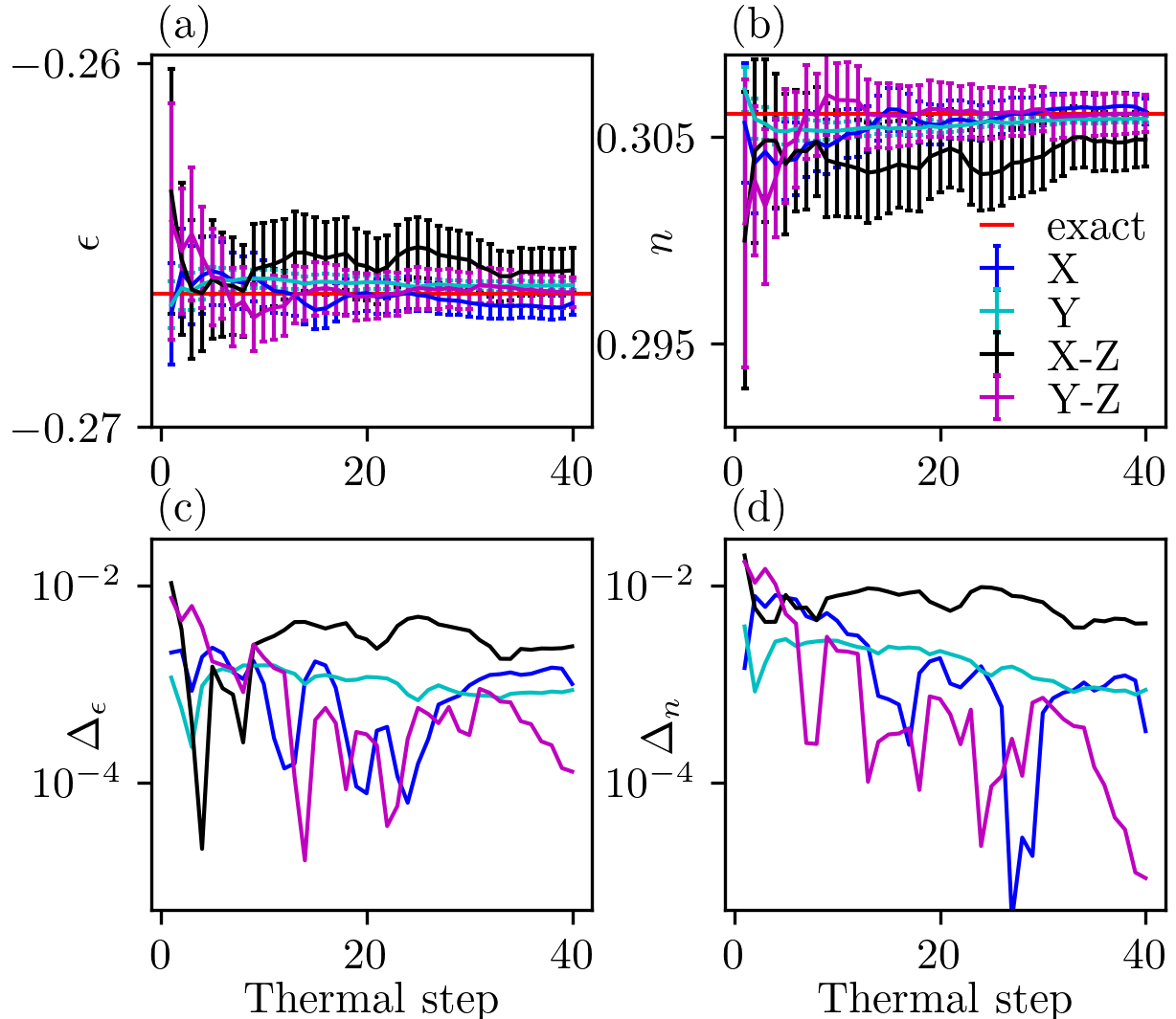
Figure 1: Classical METTS calculations of energy and particle density in the model (2) with $L=12$ at $\beta=10$ using various choices of measurement basis for state collapse. We set $h=0.1$ and $\mu=-0.4$ to reach a filling of $n=\frac{1}{3}$ in the ground state. (a) Estimated energy density $\epsilon=\frac{1}{L}\frac{1}{S_{\text{w}}k}\sum_{j=1}^{k}\sum_{i=1}^{S_{\text{w}}}\langle\phi_{ij}|\,H\,|\phi_{ij}\rangle$ as a function of thermal step $k$ with $S_{\text{w}}=100$ parallel random walks. The choices of measurement basis include $y$ (cyan line), $x$ (blue line), and alternating $xz$ (black line) and $yz$ bases (magenta line). For reference, the energy density obtained with exact diagonalization (ED) is also shown (red line). The error bars are plotted as the standard errors of $\epsilon$. (b) Same as (a) but for the particle density $n$. (c) Relative error $\Delta_{\epsilon}$ of the energy density $\epsilon$ with increasing number of thermal steps. (d) Relative error $\Delta_{n}$ of the particle density $n$. The relative error is defined as $\Delta_{\mathcal{O}}=\frac{\left|\left\langle\mathcal{O}\right\rangle_{\textrm{METTS}}-\left\langle\mathcal{O}\right\rangle_{\textrm{ED}}\right|}{\left|\left\langle\mathcal{O}\right\rangle_{\textrm{ED}}\right|}$ for a generic observable $\mathcal{O}$.

Before discussing the AVQMETTS simulations, we perform finite-temperature classical METTS calculations for the model (2) leveraging the efficiency of MPSs. The purpose is two-fold. First, as noted in Sec. II, the choice of METTS sampling basis can have a strong effect on sampling efficiency—for example the $xz$-basis collapse can outperform $z$-basis collapse as observed in Refs. [38, 44]. Moreover, in Ref. [47] it was observed in a different context that sampling infinite-temperature expectation values in the $y$-basis can be advantageous for models like Eq. (2) whose Hamiltonians contain only Pauli-$X$ and $Z$ terms. Thus we aim to study more systematically the comparative performance of collapse in various bases, including the $y$ and $x$-basis, as well as alternating $yz$ basis and $xz$ collapse bases along the lines discussed in Sec. II. We will use the optimal basis choice for subsequent classical METTS calculations and contrast the strategy for AVQMETTS, where additional constraints, such as circuit complexity measured by number of two-qubit gates, have to be taken into consideration. Second, we aim to have numerically converged calculations of the equation of state of the model (2), utilizing the efficient Trotter approach for ITE in the MPS basis. Specifically, we evaluate the energy density $\epsilon=\left\langle H\right\rangle_{\mu,\beta}/L$ and particle density $n=\left\langle N\right\rangle_{\mu,\beta}/L$ as functions of temperature and chemical potential. These calculations elucidate the physics of the 1D model and provide benchmark data for the AVQMETTS simulations presented in Sec. IV.

III.1 Optimal measurement basis for METTS collapse

Fig. 1 visualizes the estimated energy density $\epsilon$ and particle density $n$ for $L=12$ with $\beta=10$ and $\mu=-0.4$ as a function of the number of thermal steps, highlighting the dependence of convergence on several specific choices of measurement basis for METTS collapse. These data are obtained using $S_{\text{w}}=100$ parallel random walks. Figure 1(a) shows that $\epsilon$ obtained from METTS calculations with four different basis choices are generally quite close to the exact reference energy density, with relative error $\Delta_{\epsilon}\lesssim 1\%$ as shown in Fig. 1(c). For larger numbers of thermal steps, $\Delta_{\epsilon}$ is consistently smaller for calculations using the $x$-, $y$- or $yz$-bases than that using the $xz$-basis. The fluctuations of $\Delta_{\epsilon}$ with thermal steps are consistent with the standard error of $\epsilon$. The $y$-basis calculation gives the smallest standard error ($\gtrsim 0.6\times 10^{-3}$), which aligns with the minimal fluctuations of $\Delta_{\epsilon}$. This is consistent with the findings of Ref. [47] which observed that the $y$-basis displayed minimal shot-to-shot fluctuations when sampling energy-density correlation functions at infinite temperature. Similar observations apply to the calculations of particle density $n$, with slightly larger errors occuring for the $xz$-basis results, as shown in Fig. 1(b,d). In the following classical METTS simulations we choose the alternating $yz$-basis for state collapse, since calculations using this basis give consistently lower errors at large numbers of thermal steps.

III.2 Equation of state

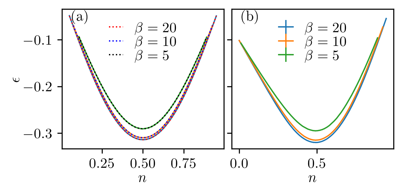
Figure 2: Energy density $\epsilon$ versus particle density $n$ equation of state obtained from METTS calculations (solid lines) on the model (2) for $L=60$ in the deconfined free-fermion limit $h=0$ (a) and in the confined phase with $h=0.1$ (b). The curves are shown for three inverse temperatures $\beta=5,10$ and $20$. The analytical results for the free fermion model are also plotted in (a) for reference as dotted lines, which agree perfectly with the respective METTS calculations.

To study the equation of state for the model (2)—i.e., the functional relationship between energy density $\epsilon$ and particle density $n$—we perform METTS calculations of a $L=60$ model with chemical potential varying from $\mu=-1.0$ to $\mu=1.0$ with a step $0.025$. The results for the free-fermion limit $h=0$ are plotted in Fig. 2(a) at three inverse temperatures $\beta=5,10$ and $20$. Without the confining field, the energy-particle density curve is symmetric around half-filling, indicative of particle-hole symmetry. Generally, the thermal energy density increases with temperature, as the number of excited states within the accessible energy window $\sim 1/\beta$ increases. As a result, $\epsilon$ grows the most at half-filling, and becomes trivially temperature-independent at zero or full filling, where the relevant subspace dimension reduces to 2 and the ground state is two-fold degenerate. For reference, the analytical calculations for the same free-fermion model are also shown in Fig. 2(a) with dotted lines, which agree perfectly with the METTS results and confirm the convergence of METTS calculations. In Fig. 2(b), we show results for the equation of state with $h=0.1$. The finite confining field clearly breaks the particle-hole symmetry. Compared with the free-fermion results in Fig. 2(a), the energy density becomes significantly lower for $n<0.5$ and reaches maximal energy reduction at $n=0$. In contrast, the variation of $\epsilon$ for $n>0.5$ is much smaller, and remains the same at $n=1$. This can be understood by considering the $\mathbb{Z}_{2}$ symmetry breaking by the confining field, which promotes the configurations with large negative magnetizations (or equivalently, those with long anti-strings as defined in Sec. III.3) and further lowers the energy. Since the total magnetization magnitude (length of anti-string) in each particle number sector is bounded by $L-2\lfloor N/2\rfloor$, the impact of the confining field on the thermal statistics grows from large filling to small filling of the model, consistent with the curves shown in Fig. 2(b). Note that the standard errors of $\epsilon$ and $n$ for these METTS calculations are below $10^{-3}$, i.e. they are are smaller than the line width of the curves.

III.3 Probes of confinement: Friedel oscillations and string length distributions

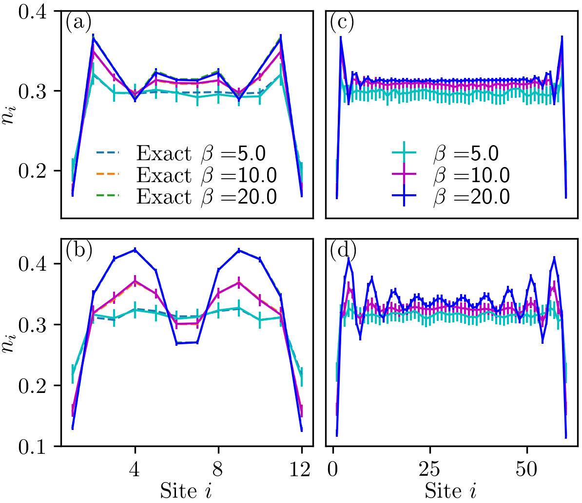
Figure 3: Friedel oscillations and their dependence on confining field and temperature. (a) Spatial distributions of single site fermion occupation numbers $\braket{n_{i}}$ (solid lines) for $L=12$ and $h=0$ at three representative temperatures $\beta=5,10$ and $20$. (b) Same as (a) but with confining field $h=0.1$. (c) Same as (a) but for $L=60$. (d) Same as (a) but for $L=60$ and $h=0.1$. We use $S_{\text{w}}=100$ random walks to generate $S_{\text{w}}\times S_{0}=2000$ METTS samples for the analysis. The particle occupation distributions obtained from exact diagonalization at $L=12$ are also shown as dashed lines in (a,b). The particle filling is set to $\frac{1}{3}$ per site at zero temperature by introducing a chemical potential $\mu=-0.55$ for $h=0$ and $\mu=-0.4$ for $h=0.1$.

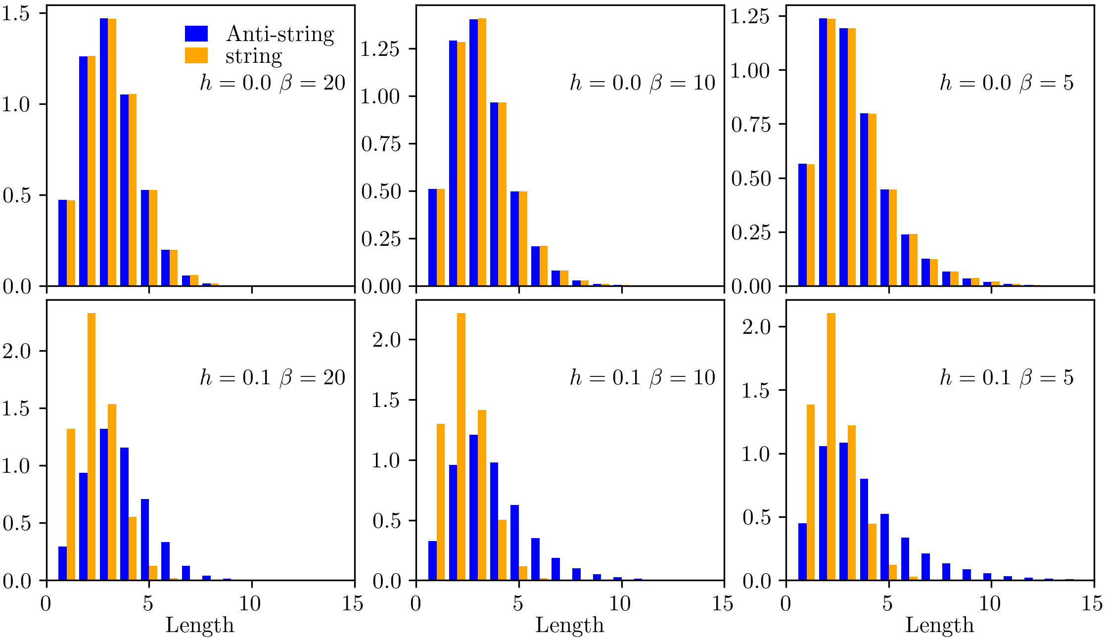
Figure 4: (Anti-)string length distribution $C_{l}$ as a function of temperature and confining field. The (anti-)string length distributions are plotted as (blue) orange histograms with $h=0$ at $\beta=20$ (a), $\beta=10$ (b), $\beta=5$ (c) and $h=0.1$ at $\beta=20$ (d), $\beta=10$ (e), $\beta=5$ (f). Calculations are performed with $L=36$ at fixed ground-state particle filling $n=1/3$. Here $C_{l}$ is evaluated for each (anti-)string length $l$ as the number of counts for that $l$ divided by the total number ($10^{5}$) of bit-string samples. Note that individual $C_{l}$s can be greater than one because there can be multiple (anti-)strings of the same length in the same bit-string.

A fundamental feature of the $\mathbb{Z}_{2}$ lattice gauge theory (1) is its manifestation of fermion confinement in both the ground state [28] and the dynamics [27]. For example, in the ground state at finite $h$, fermions form tightly bound pairs known as mesons owing to the fact that the confining field $h$ imposes an energy cost scaling linearly with the separation between fermions. This behavior is also evident in the equivalent spin model (2), where $h$ effectively counts the number of flipped spins between two Ising domain walls. One way to characterize confinement in this model is to examine Friedel oscillations in the spatial particle density distribution at specific particle fillings [28]. At zero temperature and $h=0$ the wavelength of the Friedel oscillation is simply $1/2k_{F}$, where $k_{\rm F}$ is the Fermi wavevector. In contrast, with a finite confining field, each pair of particles forms a bound state so that the wavevector reduces to $k_{\text{F}}$, leading to a doubling of the wavelength. Here we perform METTS calculations to investigate the temperature dependence of these Friedel oscillations. These calculations are complementary to simulations performed using purification approaches [33] and provide further benchmark results for AVQMETTS calculations. We set the particle filling $n=1/3$ in the ground state by tuning the chemical potential to $\mu=-0.55$ for the free fermion model and $\mu=-0.4$ with confining field $h=0.1$.

In Fig. 3, we demonstrate the Friedel oscillations by plotting the spatial distribution of site-wise particle occupations $\braket{n_{i}}$ for various temperatures and two values of the confining field. Figure 3(a) shows that there are four peaks in the spatial distribution of $\braket{n_{i}}$ at $\beta=20$ for $L=12$ and $h=0$, which corresponds to $n=1/3\times 12=4$ particles in the system. As temperature increases, the amplitude of these peaks gradually diminishes. By $\beta=5$, the two central peaks disappear. Results from calculations at finite confining field $h=0.1$ are shown in Fig. 3(b), where the number of peaks in the particle density distribution reduces to 2, as expected from the meson formation mechanism. Temperature plays a similar role and gradually washes away the peaks, suggesting a temperature-induced crossover between confined and deconfined regimes. Similar observations apply to larger system sizes readily accessible within METTS. For the $L=60$ free fermion model ($h=0$), while the Friedel oscillations near edges are visible, their amplitude is damped towards the middle of the chain, as shown in Fig. 3(c). Interestingly, the Friedel oscillations are enhanced with finite $h=0.1$, as depicted in Fig. 3(d). The ten visible peaks correspond to $n=1/3\times 60/2=10$ mesonic bound states, and the peak damps two times slower toward the center of the chain.

Another feature distinguishing the confined and deconfined regimes is the disparity in string and anti-string length distributions [33]. Here an (anti-)string refers to the consecutive 1s (0s) in a bitstring obtained from measuring a thermal state in the $z$-basis of the spin model (2); the endpoints of these (anti-)strings are Ising domain walls, which correspond to the fermions in Eq. (1). In the deconfined limit $h=0$, the length distributions are symmetric between strings and anti-strings, which reflects the $\mathbb{Z}_{2}$ symmetry in the absence of a confining field. Strings of shorter lengths become more pronounced in the confined regime. Here the confining field raises the energy cost of configurations with longer strings while lowering the energy for those with longer anti-strings, leading to the formation of mesonic bound states. In practice, to get the (anti-)string length statistics, we first collapse each of the $S_{\text{w}}\times S_{0}=2000$ METTSs $50$ times in the $z$-basis, to obtain in total $2000\times 50$ bit-strings. We then count the number of consecutive 1s (0s) in each bit-string to obtain the (anti-)string lengths. For example, in the bit-string $100111$ we would record one occurrence each for strings of length 1 and 3 and one anti-string of length 2.

Figure 4 shows the (anti-)string length distributions for an $L=36$ model at particle filling $n=1/3$ with and without confining field. In Fig. 4(a) we see that the length distributions of strings and anti-strings at $\beta=20$ are nearly identical, with a skewed distribution and a peak at $l=3$ tied to the $1/3$ particle filling. Upon increasing temperature to $\beta=10$ (Fig. 4(b)) and $\beta=5$ (Fig. 4(c)), the symmetric (anti-)string length distributions remain but are broadened due to thermal smearing effects. The string and anti-string length distributions exhibit opposite trends upon turning on the confining field $h=0.1$ as shown in Fig. 4(d). While the center of the anti-string distribution shifts to larger length $l$, the string distribution shifts to smaller $l$, consistent with the confinement effect discussed above. Increasing temperature similarly broadens the distributions as demonstrated at $\beta=10$ [Fig. 4(e)] and $\beta=5$ [Fig. 4(f)], indicating a tendency toward deconfinement.

Our results on Friedel oscillations and (anti-)string statistics at finite temperature are consistent with those obtained in Ref. [33] with a complementary MPS approach based on purifications [48, 49, 50]. The purification method computes thermal averages by preparing a state in which each physical qubit is maximally entangled with an auxiliary qubit, then performing ITE on the physical qubits for an imaginary time $\beta/2$. This method avoids the sampling entailed in METTS at the expense of doubling the number of qubits, which limits the system sizes that are easily accessible. The METTS approach adopted here allows us to simulate chains of up to $L=60$ fermion sites as in Figs. 2 and 3, whereas the finite-temperature calculations in Ref. [33] were limited to systems of $\sim 36$ sites. This increase in the accessible system sizes may be useful when studying, e.g., finite-temperature confinement phase diagrams in higher dimensions, where reducing the qubit overhead is particularly important.

IV AVQMETTS simulations

In this section, we turn to a quantum version of METTS, specifically the AVQMETTS approach [44], for finite-temperature simulations of the model (2). Here we focus on benchmarking AVQMETTS calculations of the 1D model, motivated by the intriguing physics and available exact solutions. This section is divided into three parts. We first briefly outline AVQMETTS method and its technical details. Secondly, we present our AVQMETTS numerical results concerning the finite-temperature behavior of the energy and particle densities. Finally, we give a numerical estimation of the system-size scaling for the AVQMETTS circuit complexity characterized by the number of CNOT gates, which is a useful resource estimate for near-term applications. Even though AVQMETTS is a quantum algorithm, all the following calculations are performed using a state-vector simulator, which provide important benchmarks for future AVQMETTS calculations on quantum processing units.

IV.1 The AVQMETTS method

The AVQMETTS approach adopts AVQITE [42], rather than the standard MPS-based ITE algorithms such as Trotter decomposition or time-dependent variational principle [51, 52], for METTS preparation as outlined in Sec. II. The AVQITE algorithm dynamically constructs a parameterized circuit $\left|\psi(\boldsymbol{\theta}[\tau])\right\rangle=\prod_{j}e^{-\frac{1}{2}i\theta_{j}[\tau]G_{j}}\left|\psi_{0}\right\rangle$ that closely follows the exact dynamics in imaginary time $\tau$ generated by the Hamiltonian $H$ for a CPS $\ket{\psi_{0}}$. Here, $G_{j}$ are Hermitian generators drawn from a predetermined operator pool (see below). The parameters evolve according to the equations of motion:

$$\sum_{j}g_{ij}\dot{\theta}_{j}=V_{i}\,,$$ (7)

where $g_{ij}=\text{Re}[\langle\frac{\partial\psi}{\partial\theta_{i}}|\frac{\partial\psi}{\partial\theta_{j}}\rangle+\langle\psi|\frac{\partial\psi}{\partial\theta_{i}}\rangle\langle\psi|\frac{\partial\psi}{\partial\theta_{j}}\rangle]$, also known as the Fubini-Study metric, is the real part of the quantum geometric tensor, and where $V_{i}=-\text{Re}[\langle\frac{\partial\psi}{\partial\theta_{i}}|H|\psi\rangle]$ is the energy gradient with respect to variational parameter $\theta_{i}$.

The accuracy of the variational dynamics is maintained by monitoring the McLachlan distance, $L^{2}=2(\langle\psi|H^{2}|\psi\rangle-\langle\psi|H|\psi\rangle^{2}-\sum_{i}V_{i}\dot{\theta}_{i})$ [53, 42, 54], which measures the separation between the variationally and exactly propagated states. If the McLachlan distance surpasses a preset threshold (e.g., $10^{-3}$) at a certain time step, the ansatz is expanded by appending more parameterized unitaries $\mathcal{U}_{j}$ to it until the distance threshold is met. The unitary $\mathcal{U}_{j}=e^{-\frac{1}{2}i\theta_{j}G_{j}}$ is obtained by selecting from the operator pool the generator $G_{j}$ which maximally reduces the McLachlan distance. A variety of operator pools have been explored, and the choice depends on the problem under study and can affect the convergence of AVQITE calculations [42, 55].

Before continuing we provide a few technical details about our implementation of the AVQMETTS algorithm. When propagating the variational parameters $\boldsymbol{\theta}[\tau]\to\boldsymbol{\theta}[\tau]+\boldsymbol{\dot{\theta}}\delta\tau$ according to Eq. (7), we adopt a variable time step $\delta\tau$ such that $\max_{j}|\dot{\theta_{j}}|\delta\tau$ is fixed [54], as a slight improvement in accuracy is observed compared with AVQITE simulations with a comparable fixed time step $\delta\tau=0.02$. Furthermore, we consider three different operator pools depending on the measurement basis used to collapse the METTSs. For propagating an initial CPS in the $z$-basis, the operator pool is the simplest and given by $\mathcal{P}_{z}=\{Y_{i}\}_{i=0}^{L}\cup\{Y_{i}Z_{j}\}_{0\leq i\neq j\leq L}$. For a CPS in the $x$-basis, the operator pool is expanded to $\mathcal{P}_{x}=\mathcal{P}_{z}\cup\{Y_{i}X_{j}\}_{0\leq i\neq j\leq L}\cup\{Y_{i}Z_{j}X_{k}\}_{0\leq i\neq j\neq k\leq L}$. Finally, for a CPS in the $y$-basis, we adopt an operator pool given by $\mathcal{P}_{y}=\{Z_{i},X_{i}\}_{i=0}^{L}\cup\{Z_{i}X_{j}\}_{0\leq i\neq j\leq L}\cup\{Z_{i}Z_{j}Z_{k}\}_{0\leq i<j<k\leq L}$. We constructed the $y$-basis operator pool by performing a preliminary round of calculations where we compared the fidelity between CPSs evolved under AVQITE and under exact ITE, and we selected those Pauli operators generating the highest fidelity. Note that multiple operator pools will generically be used in the course of an AVQMETTS calculation with a collapse basis that alternates between thermal steps as described in Sec. II.

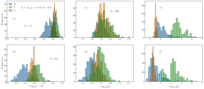
Figure 5: Benchmarking the accuracy of AVQITE calculations for initial CPSs in the $x$, $y$, and $z$-basis. (a) Histogram of the infidelities $1-\mathcal{F}$ at $\beta=1$. (b) Same as (a) but at $\beta=2$. (c) Histogram of the relative errors of the energy $E=\langle H\rangle_{\text{AV}}$ at $\beta=1$. (d) the same as (c) but at $\beta=2$. (e) Histogram of the relative errors of the particle filling $\langle N\rangle_{\text{AV}}$ at $\beta=1$. (f) the same as (e) but at $\beta=2$. We consider a random sample of initial CPSs of size $\mathcal{M}=288$ in each basis. The Hamiltonian parameters are set to $L=12$, $\mu=-0.55$, and $h=0$ to yield a ground state at $n=1/3$ filling.

IV.2 Benchmarking the impact of CPS collapse basis

As discussed in Sec. III, the choice of collapse basis plays an important role in the METTS sampling procedure. However, this choice must be re-evaluated in the context of AVQMETTS, which uses AVQITE as the CPS propagation subroutine. For example, the performance and quantum resource requirements of AVQITE simulations depend on the choice of reference state $\ket{\psi_{0}}$, which in the context of AVQMETTS calculations can be a product state in the $x$, $y$, or $z$ basis depending on the choice of collapse basis. To explore this dependence, we benchmark the accuracy of AVQITE simulations of the model (2) in comparison with ITE via exact diagonalization. We consider a system of size $L=12$ in the free-fermion limit ($h=0$) and with a chemical potential of $\mu=-0.55$, such that the ground state has four particles (1/3 filling). We then randomly select $\mathcal{M}=288$ CPSs in each of the three ($x/y/z$) measurement bases, and evolve them using both AVQITE and exact ITE up to an imaginary time $\beta/2$. We consider two figures of merit for the accuracy of AVQITE simulations relative to exact ITE. First, we consider the infidelity $1-\mathcal{F}=1-\left|\left\langle\psi(\beta)_{\textrm{AV}}\right.\left|\psi(\beta)_{\textrm{ITE}}\right\rangle\right|^{2}$ of the AVQITE state $\left|\psi(\beta)_{\textrm{AV}}\right\rangle$ with respect to the exact ITE state $\left|\psi(\beta)_{\textrm{ITE}}\right\rangle$. Second, we consider the quantity $\tilde{\Delta}_{\mathcal{O}}=\left|\left\langle\mathcal{O}\right\rangle_{\textrm{AV}}-\left\langle\mathcal{O}\right\rangle_{\textrm{ITE}}\right|/\left|\left\langle\mathcal{O}\right\rangle_{\textrm{ED}}\right|$, where $\braket{O}_{\rm ED}$ is the thermal average of $\mathcal{O}$ obtained from exact diagonalization. This quantity can be interpreted as measuring the absolute difference between AVQITE and exact ITE in units of the exact thermal expectation value $\braket{\mathcal{O}}_{\rm ED}$, which is more natural than $\braket{\mathcal{O}}_{\rm ITE}$ itself as this quantity can be close to zero even when $\braket{\mathcal{O}}_{\rm ED}$ is finite. (Note that the average value of $\braket{\mathcal{O}}_{\rm ITE}$ is not the same as the METTS estimate of $\braket{\mathcal{O}}$ because it samples the METTS uniformly.) For this metric, we consider as observables the energy density $\epsilon$ [calculated with respect to the Hamiltonian (2)] and the particle density $n$ [calculated with respect to the number operator (4)].

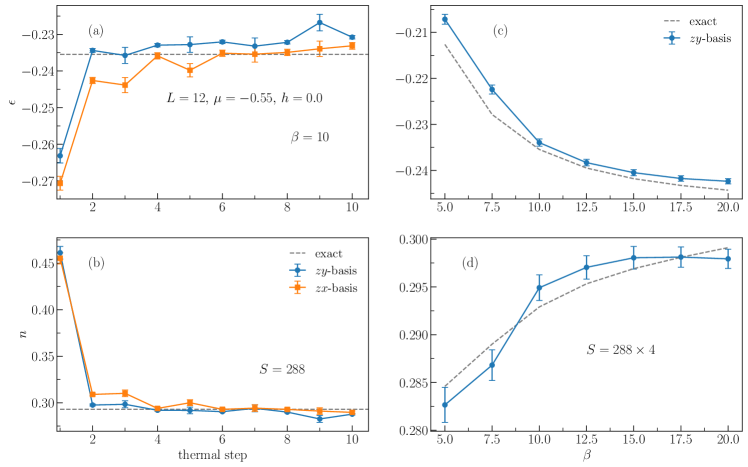
Figure 6: Minimal autocorrelation between thermal steps and accuracy of thermal energy and particle density from AVQMETTS calculations on the model (2) at $L=12$ without a confining field ($h=0$), and with a chemical potential set to $\mu=0.55$, which gives 1/3 particle filling. (a) Thermal energy density $\epsilon$ as a function of thermal steps using the alternating $yz$-basis (blue circles) at $\beta=10$. The results using $xz$-basis (orange squares) are also shown for comparison, together with the exact thermal energy density (dashed line). Each thermal step result represents an average over $S_{w}=288$ independent random walks. (b) Same as (a), but for particle density $n$. (c) Thermal energy density as a function of $\beta$ from AVQMETTS calculations using $yz$-basis, in comparison with exact results. The AVQMETTS result at each temperature is an average over $S_{w}\times S_{0}=288\times 4$ samples. (d) Same as (c) but for particle density.

Figure 5 shows the distribution of the above figures of merit over the $288$ initial CPSs per product state basis for inverse temperatures $\beta=1$ (top panels) and $\beta=2$ (bottom panels). While all the infidelities are smaller than $10^{-2}$ as shown in Fig. 5(a,b), the infidelities of the METTSs from AVQITE calculations are smallest when the initial CPSs are $z$-basis states, followed by those in the $y$- and $x$-basis, respectively. When $\beta$ increases from $1$ to $2$, the infidelities generally increase as well due to error accumulations from taking more imaginary-time steps of similar step size. Nevertheless, this trend of increasing infidelities with $\beta$ does not necessarily persist to low temperatures, as demonstrated in Ref. [44], which is also corroborated by the accurate AVQMETTS calculations at low temperatures ($\beta=5,10,20$) to be reported later. In Fig. 5(c) we show the distributions of $\tilde{\Delta}_{E}$ for AVQITE calculations starting from the three initial CPS bases, all of which roughly peak around $10^{-1.8}\simeq 1.6\%$ at $\beta=1$. At larger $\beta=2$ as shown in Fig. 5(d), the distribution of $\tilde{\Delta}_{E}$ of the three groups are more separated, where the peak position shifts to $10^{-1.75}\simeq 1.8\%$ for $z$-basis results, $10^{-1.7}\simeq 2.0\%$ for $y$-basis, and $10^{-1.6}\simeq 2.5\%$ for $x$-basis. The trend correlates well with that of the infidelities. Fig. 5(e,f) plots the distributions of $\tilde{\Delta}_{N}$ for $\beta=1$ and $2$, respectively. Here, the $z$-basis results have significantly smaller error as compared to the $x/y$-basis results. This can be understood by noting that the initial CPSs in the $z$-basis are eigenstates of the particle number operator $N$, which also commutes with the Hamiltonian $H$. Therefore, in principle, ideal ITE under $H$ only propagates these states within a fixed-particle number sector. Numerically, about $25\%$ of the 288 AVQITE results in the $z$-basis yield $\tilde{\Delta}_{N}=0$ (these values are not included in the histograms). The small but finite values of $\tilde{\Delta}_{N}$ for the $z$-basis results in Fig. 5(e,f) imply a slight symmetry-breaking in the AVQITE calculations. The $\tilde{\Delta}_{N}$ distribution of $x$-basis results appears broader than for the $y$-basis results, but with a roughly similar peak position. Overall, the particle number results are more accurate than the energy results.

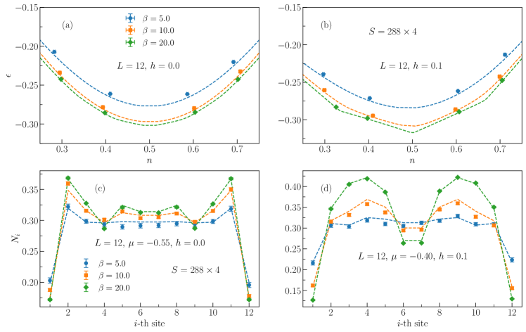
Figure 7: AVQMETTS calculations of energy density and particle number distribution. (a) Energy density $\epsilon$ as a function of particle number density $n$ for a free-fermion system (h=0) of size $L=12$ at inverse temperatures $\beta=5,10,20$. (b) Same as (a) but for a finite confining field $h=0.1$. We choose chemical potential values $\mu\in(-0.6,0.6)$ to get 4 points (symbols) at each temperature and compare them with exact calculations (dashed curves). (c) Particle occupation $n_{i}$ as a function of site $i$ for $L=12$ and $h=0$ from AVQMETTS calculations (symbols), with comparison to exact results (dashed lines). (d) Same as (c) but for $h=0.1$. The chemical potential is set to $\mu=-0.55$ in (c) and $\mu=-0.40$ in (d) to yield $1/3$ particle filling in the ground state. Each AVQMETTS calculation generates $S_{w}\times S_{0}=288\times 4$ samples for thermal averaging.

From the previous discussion one may argue in favor of AVQMETTS simulations using only the $z$ basis for state collapse, as Fig. 5 demonstrates that AVQITE simulations for CPSs in the $z$ basis give the best accuracy overall. However, it is also important to consider the sampling efficiency for the thermal average of an observable $\mathcal{O}$, which is tied to the spread of the distribution of $\langle\mathcal{O}\rangle_{i}$ over METTSs with respect to the exact thermal average $\langle\mathcal{O}\rangle_{\textrm{ED}}$. High sampling efficiency is expected if the distribution is narrowly peaked around $\langle\mathcal{O}\rangle_{\textrm{ED}}$. Note that, as mentioned above, the average of $\langle\mathcal{O}\rangle_{i}$ over METTS obtained from $\mathcal{M}$ uniformly sampled CPSs need not converge to $\langle\mathcal{O}\rangle_{\textrm{ED}}$. We therefore define the following measure of relative error with respect to the exact thermal average:

$$\mathcal{D}_{\mathcal{O}}=\frac{1}{\mathcal{M}}\sum_{i=1}^{\mathcal{M}}\left|\left(\mathcal{O}_{i}-\langle\mathcal{O}\rangle_{\textrm{ED}}\right)/\langle\mathcal{O}\rangle_{\textrm{ED }}\right|\,,$$ (8)

which measures the spread of the distribution of $\langle\mathcal{O}\rangle_{i}$ relative to $\langle\mathcal{O}\rangle_{\textrm{ED}}$.

Table 1 shows the spread of the energies $\langle H\rangle_{i}$ and particle numbers $\langle N\rangle_{i}$ characterized by $\mathcal{D}_{E}$ and $\mathcal{D}_{N}$ from both AVQITE (bold numbers) and exact-ITE calculations. We used the same $\mathcal{M}=288$ states as in Fig. 5 to generate this table. The values obtained from AVQITE calculations are very close to those from exact-ITE, which further corroborates the accuracy of AVQITE. Across two representative temperatures ($\beta=1,2$), one can see that calculations using the $y$ basis consistently produce the smallest $\mathcal{D}_{E}$ and $\mathcal{D}_{N}$, while results using $z$($x$)-basis states are smaller for $\mathcal{D}_{E}$ ($\mathcal{D}_{N}$).

	$\mathcal{D}_{E}(\%)$			$\mathcal{D}_{N}(\%)$
	$X$	$Y$	$Z$	$X$	$Y$	$Z$
$\beta=1.0$	$\mathbf{4.06}$ 3.99	$\mathbf{0.40}$ 0.38	$\mathbf{1.53}$ 1.53	$\mathbf{0.29}$ 0.29	$\mathbf{0.09}$ 0.09	$\mathbf{2.80}$ 2.80
$\beta=2.0$	$\mathbf{2.25}$ 2.12	$\mathbf{0.47}$ 0.42	$\mathbf{1.40}$ 1.42	$\mathbf{0.96}$ 0.92	$\mathbf{0.17}$ 0.17	$\mathbf{4.17}$ 4.17

Table 1: The spread of energy and particle number distributions for METTSs with respect to exact thermal averages, as measured by $\mathcal{D}_{E}$ and $\mathcal{D}_{N}$ (8), at two different temperatures $\beta=1,2$. We choose random samples of $\mathcal{M}=288$ CPSs in each of the three ($x/y/z$)-basis representations, which are evolved up to $\beta/2$ using both AVQITE and exact-ITE for the analysis.

Even though the AVQITE simulations for the CPSs in the $y$ basis yields the narrower energy and particle number distributions relative to the exact thermal averages (which implies better sampling efficiency for AVQMETTS), in practice, alternating the measurement basis for METTS collapse is found to reduce autocorrelation effects between thermal steps [38, 44]. Given the better AVQITE simulation accuracy for CPSs in the $z$-basis as demonstrated in Table 1 and the associated smaller $\mathcal{D}_{E}$, we choose the $yz$-basis for AVQMETTS, where calculations alternate between $y$- and $z$-basis measurements at odd and even thermal steps, respectively. To demonstrate the effectiveness of the $yz$-basis for AVQMETTS simulations, we plot in Fig. 6(a,b) the energy and particle number densities as functions of the number of thermal steps at $\beta=10$. Minimal autocorrelation effects are observed, as the thermal averages already converge to the exact thermal expectation values (dashed lines) at the second thermal step subject to fluctuations tied to the sample size $S=288$. This suggests that it suffices to skip the first thermal step for each Markovian random walk in AVQMETTS to get a METTS ensemble to estimate thermal averages. We follow this procedure for the following calculations. For reference, we also show the results with the $xz$-basis as adopted in Refs. [38, 44], where the calculations use an alternating $x$- and $z$-basis for collapse. One can see a faster convergence for $yz$-basis calculations compared with $xz$ results, especially for the energy density. In Fig. 6(c,d) we show the AVQMETTS estimates of thermal energy and particle density as functions of $\beta$ with $S=288\times 4$ samples. They agree well with the exact results up to a relative error of at most $2.6\%\ (0.8\%)$ for energy (particle) density.

IV.3 AVQMETTS simulations of energy and particle densities

With the important simulation parameters for AVQMETTS optimized through the analyses above, we proceed to benchmark calculations of the equation of state and Friedel oscillations of the spatial particle density distribution.

In Fig. 7(a) we plot the energy density as a function of the particle number density for the model (2) at $L=12$ and without confining field ($h=0$). The AVQMETTS results (symbols) agree well with the exact diagonalization results (dashed curves) at three representative temperatures $\beta=5,10,20$. The deviations become slightly bigger when temperature increases ($\beta$ reduces), which can be attributed to the fact that we use a fixed ensemble size of $S_{w}\times S_{0}=288\times 4$. The maximal relative error is estimated to be $\Delta_{\epsilon}=3\%$ at $\beta=5$ by aligning $n$ with the exact result. As discussed in Sec. III.2, the finite confining field breaks the particle-hole symmetry of the model, which might make the AVQMETTS simulations more challenging. Nevertheless, as we show in Fig. 7(b), the accuracy of energy and particle density remains equally good with finite confining field $h=0.1$. In these calculations, we selected four values of the chemical potential in $\mu\in[-0.6,0.6]$ to obtain particle density points in the vicinity of half filling ($n=0.5$).

We further present the spatial distribution of the particle density $\langle n_{i}\rangle$ of the model without confinement in Fig. 7(c), which shows Friedel oscillations with a number of peaks equal to the particle occupancy $\langle N\rangle$, as discussed in Sec. III.3. Here one can the AVQMETTS results (symbols) also agree well with the exact results (dashed lines), where the four peaks are well resolved. As above, the deviation becomes slightly bigger with increasing temperature due to our use of a fixed ensemble size. At $\beta=5$ where the oscillations are almost washed out, the maximal relative error is about $\Delta_{n_{i}}=4.2\%$. Here we set $\mu=-0.55$ such that the system has $4$ particles in the ground state, consistent with calculations in Sec. III.3. We also find a consistent accuracy for the particle density distribution with finite confining field ($h=0.1$), where the number of peaks reduces to two due to particle pairing, as shown in Fig. 7(d).

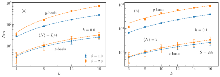
Figure 8: System-size dependence of the AVQMETTS ansatz circuit complexity as measured by the number of CNOT gates $N_{\textrm{CX}}$. (a) Growth of $N_{\textrm{CX}}$ as a function of the system size $L$ for the deconfined free-fermion model with $h=0$. The results are shown for the two alternating $y$- and $z$-measurement basis for METTS collapse at temperatures $\beta=1,2$. Here we select a chemical potential $\mu$ for each system size to maintain a total filling $\langle N\rangle=L/4$ in the ground state. (b) Same as (a) but with confining field $h=0.1$ and with the chemical potential chosen to maintain a constant ground-state particle number $\langle N\rangle=2$ for all $L$. Each data point corresponds to an average over 288 random CPSs in the $y$ or $z$-basis. Dashed lines are best fits of the data with the function $f(L)=aL^{b}$.

IV.4 System-size scaling of AVQMETTS circuit complexity

Even though the AVQMETTS calculations above are performed on classical statevector simulator, we have access to the circuit representation and can therefore estimate the circuit complexity characterized by the number of CNOT gates $N_{\textrm{CX}}$ used in the variational ansatz circuits at the end of the ITE process. For simplicity, we assume here a QPU with all-to-all qubit connectivity, which applies to trapped-ion devices. Thereby, for a given AVQITE ansatz with $N_{\theta}$ unitaries each of which has an angle $\theta_{j}$ associated with a Pauli string $G_{j}$ as a generator, we can estimate $N_{\textrm{CX}}$ as:

$$N_{\textrm{CX}}=\sum_{j=1}^{M}2\left(W_{j}-1\right),$$ (9)

where $W_{j}$ is the weight (number of nonidentity Pauli operators) of the Pauli string $G_{j}$.

In Fig. 8(a) we show the statistics of $N_{\textrm{CX}}$ (symbols) for AVQITE circuits with initial CPSs in the $y$ and $z$ bases as a function of system size $L$. Here the confining field is set to $h=0$, and the chemical potential $\mu$ is adjusted such that the total fermion filling $\langle N\rangle=L/4$. We apply AVQITE to propagate the CPSs up to a temperature $\beta=1,2$. The dashed lines show that they can be fitted well by a simple power-law function $f(L)=aL^{b}$, with exponent $b$ ranging from $1.6$ to $2.1$ for the different measurement basis and temperature values considered here. One can clearly see a bimodal distribution of AVQITE calculations: $N_{\textrm{CX}}$ for AVQITE calculations starting from $z$-basis CPSs is in the range of $[4,30]$, while that of $y$-basis in $[20,800]$, demonstrating over an order of magnitude increase at fixed $L$. Furthermore, increasing $\beta$ at fixed $L$ leads to only a slight increase in $N_{\textrm{CX}}$ for $z$-basis results, in contrast to the substantially larger increase observed for the $y$-basis results. Fig. 8 shows that $N_{\textrm{CX}}$ displays a modest up-shift as we change the confining field from $h=0$ to $h=0.1$; the maximal $N_{\textrm{CX}}$ rises from $32$ to $34$ for the $z$-basis results, and from $740$ to $900$ for $y$-basis results. Hence, even though we showed in Table 1 that the $y$-basis samples are more concentrated around the thermal average, the implied greater sampling efficiency can be compromised by the increased quantum resource overhead in AVQMETTS calculations. This again suggests that AVQMETTS using the alternating $yz$-basis for state collapse may be an optimal choice.

V Conclusion

In this paper we investigated the utility of METTS approaches to the simulation of gauge theories at finite temperature and density. The METTS approach is useful both in classical simulations of quantum matter via tensor network approaches and is a promising candidate for implementing finite-temperature simulations on quantum computers via, e.g., AVQMETTS. We focused on the simplest lattice model of a gauge theory coupled to matter, the one-dimensional $\mathbb{Z}_{2}$ gauge theory, and demonstrated the applicability of METTS techniques to study the finite-temperature and -density equation of state as well as signatures of fermion confinement. We investigated systematic issues common to both the classical and quantum implementations of METTS, particularly the impact of CPS collapse basis on the sampling complexity. We also benchmarked the impact of sampling basis on the AVQITE quantum ITE subroutine in terms of both simulation accuracy and quantum resource cost. Our study demonstrates that METTS approaches are capable of accurately simulating the confined and deconfined regimes of the model in a large range of temperatures and system sizes. We performed classical METTS simulations of 1D chains at system sizes exceeding those accessible to purification approaches [33], as well as of smaller systems more likely to be the subject of near-term quantum computing studies. We find that an optimal choice of sampling basis can speed up convergence of the METTS sampling, but also demonstrate a cautionary observation that the best sampling basis may lead to unfavorable circuit complexity scaling in a quantum computing setting. We suggest an alternating collapse basis approach to exploit the advantages of different bases that we expect will prove useful in future studies.

The methods adopted in this work to calculate the equation of state may offer insight into two topics of current interest in the study of neutron matter, namely neutron star mass-radius relations [56, 57, 58, 59] and multi-messenger signals of neutron star mergers [60, 61, 62, 63, 64]. Both require a knowledge of the equation of state of nuclear matter at finite density and temperature. In the case of the former, neutron stars data which favors a soft equation of state at low density and a stiff one at high density is in tension with several theoretical models which predict a rather soft equation of state at high density [65]. In fact this soft-stiff equation of state data from neutron stars suggests that the speed of sound is non-monotonic as a function of density. Since first-principles QCD calculations are currently out of reach, it is worthwhile exploring whether toy models in lower dimensional theories like the one studied in this work can exhibit some of these features expected in the QCD equation of state. Similarly, nuclear/QCD equations of state at relatively higher temperature are used in numerical relativity simulations to predict gravitational wave signals from neutron star merger events. Computing finite temperature equations of state for toy models is a step towards eventually doing the same for QCD. By investigating the systematics of (AVQ)METTS calculations, our paper lays the groundwork for both classical and quantum computers to tackle these questions in the future.