Coarse-grained dynamics in quantum many-body systems using the maximum entropy principle
Abstract
Starting from a coarse-grained map of a quantum many-body system, we construct the inverse map that assigns a microscopic state to a coarse-grained state based on the maximum entropy principle. Assuming unitary evolution in the microscopic system, we examine the resulting dynamics in the coarse-grained system using the assignment map. We investigate both a two-qubit system, with swap and controlled-not gates, and -qubit systems, configured either in an Ising spin chain or with all-to-all interactions. We demonstrate that these dynamics exhibit atypical quantum behavior, such as non-linearity and non-Markovianity. Furthermore, we find that these dynamics depend on the initial coarse-grained state and establish conditions for general microscopic dynamics under which linearity is preserved. As the effective dynamics induced by our coarse-grained description of many-body quantum systems diverge from conventional quantum behavior, we anticipate that this approach could aid in describing the quantum-to-classical transition and provide deeper insights into the effects of coarse-graining on quantum systems.
1 Introduction
Coarse-grained descriptions of quantum systems have been extensively used to study many-body quantum systems. These effective descriptions are essential because full quantum descriptions are impractical. Coarse-grained descriptions work by reducing the number of degrees of freedom, making the analysis more manageable [1]. This framework has also been pivotal in studying the quantum-to-classical transition [2], which remains, alongside the measurement problem, an active area of research due to the inherent linearity of the theory and the mathematical connections between the studied entities and the outcomes of measurement [3, 4, 5].
Recently, coarse-grained descriptions have been employed to understand processes such as the thermalization of closed quantum systems, and efforts to investigate the dynamics of these systems have revealed that effective dynamics are not of Kraus form [6]. Moreover, non-linear, non-Markovian quantum dynamics have been observed to arise from coarse-grained descriptions, though often in an ad-hoc setting [7], highlighting the need for a more comprehensive study.
A recent framework developed to study quantum many-body systems using imperfect measurements offers a more general approach to extending the study of such dynamics [8]. This work aims to address this need by exploring the characteristics of the dynamics of a quantum system described through this coarse-grained model. This model accounts for the possibility of measuring different particles than intended and incorporates a lack of resolution in the detection apparatus.
The challenge arises when only coarse-grained information is accessible—how can one determine the specific microscopic state that is being propagated? Indeed, the observed state may correspond to numerous microscopic states. To tackle this, we construct an assignment map that links the coarse-grained state to a single microscopic state using the maximum entropy principle. This principle has been previously employed to assign a description to a quantum system based solely on its coarse-grained description [7, 9].
In our work, we assume that the observer is not aware of the number of particles in the microscopic system and only has access to the information provided by the aforementioned coarse-grained model. Using the maximum entropy assignment map, the assigned microscopic state is evolved according to Schrödinger’s equation, allowing for an effective evolved state to be recovered through the coarse-grained description of the evolved -body system. The resulting effective dynamics, that is, the dynamics observed in the coarse-grained space, is the focal point of our study. We apply this formalism to the context of quantum computing, where we study the effective dynamics of a two-qubit system that evolves under SWAP and CNOT gates. We also explore the effective dynamics of a -particle spin- chain, with different interaction configurations. This approach not only provides insights into the effective dynamics of quantum systems but also offers potential applications in understanding the quantum-to-classical transition.
The paper is organized as follows. First of all, in section 2 we introduce both the coarse graining map and the maximum entropy assignment map, so that we can mathematically construct the effective dynamics of the macroscopic system. Then we apply these tools to different microscopic evolutions. In particular, section 3 is devoted to the study of the effective dynamics of a two-qubit system with underlying SWAP and CNOT gates. In section 4, we explore the effective dynamics of a -qubit system configured as an Ising spin chain, with both all-to-all and nearest-neighbor interactions. Finally, in section 5, we establish conditions for general microscopic dynamics under which linearity is preserved, and we present an example of a microscopic dynamics that preserves linearity, but is nonetheless non-Markovian.
2 Effective dynamics in coarse-grained systems
In this section we introduce the coarse graining map from which the effective description of the state is recovered. Next, we construct the maximum entropy assignment map that will be used to assign a microscopic state to the effective state, and study some of its properties. This map is used to formally present the effective dynamics in a quantum many-body system subject to a coarse grained description.
2.1 The coarse graining map
Consider an imperfect measuring device that is subject to two types of errors. First, the device lacks the capability to accurately distinguish between the individual particles of a -level -body system. In other words, there exists a non-zero probability of wrongly identifying particles according to a permutation . This type of measurement is referred to as a fuzzy measurement. Second, the device does not have the ability to resolve all particles; only a subset of particles can be measured. Mathematically, a partial trace over the complement of is performed. A coarse-grained description of the system is obtained when both types of error are combined [8], in the sense that expected values should be calculated with respect to an effective state resulting from the application of the coarse-graining map
| (1) |
where represents the partial trace over the complement of , and is the space of bounded linear operators acting on .
Our primary focus is directed towards a particular case of the coarse graining map given by (1). First, the measuring device might mistakenly swap pairs of particles. Second, it is able to resolve a single particle, that is . Without loss of generality, we can assume that the first particle is the one that is intended to be measured, so that The coarse graining map that captures this situation is
| (2) |
where is the permutation between the first and the -th particle, and . If a state tomography were to be performed on the system using our imperfect apparatus, the result would be a one-particle effective state ; similarly the expected value of any single particle observable will be . It is crucial to recognize that the resulting effective state is a mixture of all the reduced systems of the microscopic system (assuming ).
Two specific probability distributions hold particular significance in this context:
| and | (3) |
The first one represents the scenario in which the measuring device is completely incapable of distinguishing between the individual particles. This situation is akin to a gas, where each particle has an equal probability of being found anywhere within the system. The second one can be interpreted as the first particle being the one that is closest to the measuring device and the other providing a mean background noise. These distributions are referred to as the non-preferential and preferential distributions, respectively.
2.2 Maximum entropy principle and the assignment map
Now let us shift our attention to the assignment map, which allows us to make an inference about the microscopic state of the system through our coarse-grained measurements. It is through this map that we will be able to obtain the state that will evolve according to the microscopic dynamics. The assignment map is constructed by selecting the microscopic state that maximizes the von Neumann entropy, while ensuring that it corresponds to the effective macroscopic state under a specific coarse-graining map, in a similar spirit as [10, 11] or in the context of coarse graining [6, 9]. The maximization of entropy is carried out using the method of Lagrange multipliers, where the information of the effective state will be used as constraints.
Let us assume that we are able to perform a state tomography on the effective state [12]. If is a tomographically complete set of operators acting on the Hilbert space of the effective state , then their expected values can be connected to the expected values of a set of operators acting on the Hilbert space of the microscopic state, . These operators are defined by
| (4) |
where is the operator acting on the -th particle. This connection is expressed mathematically by
| (5) |
and is studied in appendix A. Notice that the operators can be thought as fuzzy operators since they are equivalent to applying the operator to the -th particle with probability . Note that the set is not tomographically complete, implying that we do not have access to all the details about the microscopic system.
Given the expected values of the operators, the state that maximizes the von Neumann entropy is then
| (6) |
where is the Lagrange multiplier associated to the expectation value . Indeed,
| (7) |
with the partition function being
| (8) |
Because the operators in equation (6) commute, it is easy to observe that the maximum entropy state is separable. Due to this property, the maximum entropy assignment map is
| (9) |
where is the partition function associated with the -th particle, and is the set of density matrices acting on . The dependence of the assigned state on the effective state is encoded in the parameters. In fact, given the effective state , the parameters are obtained by noting that the norm of the generalized Bloch vector of the effective state, , can be expressed as
| (10) |
where
| and | (11) |
Thus, inverting (10) we can find all the parameters from . More precisely
| (12) |
where is the component of the Bloch vector. Now, the assigned states by the maximum entropy assignment map in the preferential and non-preferential cases (3) are
| (13) | ||||
| (14) |
respectively. In the preferential case, (13), we have defined the reduced state of the non-preferential particles as
| (15) |
2.3 Complete positivity of the assignment map
One might wonder if the assignment map is completely positive. Since this map is non-linear, its extension to a higher space is not direct. To build the extension, we resort to the physical definition, namely that we look for a maximum entropy state compatible with the physical constrains. Following this reasoning, complete positivity will be derived.
Consider a dilation of the microscopic description of the system with an ancillary system described by the Hilbert space ; since the extended coarse graining map does not change the dimension of the extension, we will use also for the dilation of the coarse-grained description. Thus, the total state of the extended microscopic system is , where is the Hilbert space of the microscopic description of the original quantum system. The next step is to extend the observables of the coarse-grained description:
such that , with , the effective extended state.
Since the assignment map consist of preparing the maximum entropy state compatible with the known expected values of , the following expression holds,
with defined in eq. (4) and is the maximum entropy state compatible with the mean values defined above. To construct explicitly using the operators , first observe that , therefore . Thus and the s coincide with the ones in eq. (12). Therefore the following holds,
with . This result is expected considering that the given expected values do not give any information about the ancillary system. The map corresponds to the assignment map compatible with the coarse graining map , and can be regarded as the dilation of . Moreover, it is clearly positive for any , which proves its complete positivity.
Observe that is not written in the usual fashion “” as it is non-linear, but we were able to construct the extension anyway given that we can perform the preparation of the maximum entropy state compatible with the local observations, for any extension of the system.
2.4 The effective dynamics
Now that we have established the use of a coarse graining model that incorporates both resolution and permutation errors, and have constructed an assignment map based on the maximum entropy principle, we can explore the evolution of the effective system. Since we assume that the state that propagates due to the underlying evolution is precisely the one assigned via the maximum entropy assignment map, we can represent the dynamics of the effective state through the following commutative diagram
where is the evolution of the microscopic state. The evolution of the effective state can be thus obtained from the composition three different operations [7]. First, a microscopic state is assigned to the effective state through the MaxEnt assignment map. Then, the assigned map is propagated via . Finally, we define the coarse-grained description of the evolved assigned state to be the evolved effective state. In this way, we define the coarse-grained dynamics as the composition
| (16) |
Unlike the dynamical maps typically studied in the theory of open quantum systems, the effective dynamics is typically non-linear, although it still maps quantum states to quantum states. Moreover, is a (non-linear) completely positive trace preserving map (non-linear CPTP), since the assignment map is CPTP, and are already linear CPTP maps, and the concatenation of CPTP maps is CPTP. The nonlinearity is inherited from the nonlinearity of the assignment map. In the next sections we shall explore examples of effective dynamics that can result in multi-qubit systems.
3 Effective non-linear quantum gates
In light of the framework we have developed, and before examining the effective dynamics of -qubit systems, we will focus our attention on simpler two-qubit systems, where the effect of the coarse graining map on a microscopic state will be
| (17) |
which is a convex combination of the reduced states of the two qubits, and it’s equivalent to equation (2) for . In particular, we will explore the effective dynamics generated by two well known quantum gates: the swap gate and the cnot gate. We will see that the resulting effective dynamics is far from uninteresting. Indeed, the effective dynamics induced by these gates exhibit non-linearity and non-Markovian behavior [13].
3.1 Effective SWAP gate
The Hamiltonian given by
| (18) |
has the property of generating the SWAP gate for . Following the definition of , eq. (16), we find that the effective state of the evolved system is given by
where is the unitary operator generated by the Hamiltonian (18). Since the effective initial state is given by equation (17), it is possible to see that the effective state’s Bloch vector has a constant direction, only its length changes with time. This means that the effective dynamics corresponds to a depolarization channel where the depolarization coefficient depends on the initial state. To facilitate our analysis, let’s define the Bloch vector’s norm for the -th particle as , and similarly, denote the norm of the Bloch vector for the effective state as . With this, the quotient between the norm of the Bloch vector of the initial effective state and the norm of the Bloch vector of the effective state at time is given by
| (19) | ||||
This allows us to write the effective dynamics of the system as
| (20) |
Furthermore, since the effective dynamics is a depolarization channel, the evolution of the effective state is described by the following Lindblad-like differential equation
| (21) |
A plot of the decay rate and the depolarization coefficient is shown in figure 1. This reveals that there are some scenarios where the effective state remains unchanged over time. For example, in the non-preferential case where , the microscopic state is invariant under the swap gate (see equation (14)), and therefore the effective state remains invariant under the effective dynamics. In fact, it is easy to see that the depolarization coefficient (19) is equal to one when (which is also shown in figure 1).
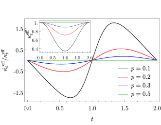
Additionally, all pure states are also invariant under the effective dynamics, as long as no , since the only microscopic states compatible with such macroscopic state is , a symmetric state. More interesting than all, the decay rate is able to take negative values, indicating that, in addition to being non-linear, the effective dynamics is non-Markovian [14, 15, 16, 17]. This is a result of information flowing back and forth between the different subsystems. This does not mean, however, that the process is reversible, as information is lost due to the coarse graining map.
3.2 Effective CNOT gate
Similarly to (18), the Hamiltonian
| (22) |
generates the cnot gate at time . The effective dynamics at an arbitrary time might be found by following the same procedure as in the previous case. However, the resulting expression is cumbersome and not very illuminating. Instead, we will focus on the effective dynamics of the system at the time , which is the time at which the cnot gate is generated. The effective dynamics at this time is given by
| (23) | ||||
where is a dephasing channel along the direction with dephasing coefficient . For example, if , then
| (24) |
That is, in (23), we encounter a convex combination of the effective state and two non-linear state-dependent dephasing channels. Note that the usual interpretation of the cnot gate is recovered, as we see that bit-flip (phase-flip) is applied to the second (first) particle depending on the state of the first (second) particle. At an arbitrary time , the effective dynamics is given by
| (25) |
where
and
In appendix B we show that and are channels that describe elliptical trajectories on the Bloch sphere. This is because they correspond to the reduced dynamics of two two-level systems that evolve according to a non-local Hamiltonian [18].
4 Effective spin chain dynamics
Now that we have seen that non-linear, non markovian results arise from the coarse-grained dynamics of a two-qubit system, we study larger many-body systems, such as the spin chains.
4.1 Non uniform external magnetic field with all-to-all interactions
First, we will consider spin one-half chains evolving in a non-uniform external magnetic field in the direction with an all-to-all Ising interaction parallel to the field. The Hamiltonian considered is thus
| (26) |
where
| (27) |
Since the field and interaction terms commute, it is possible to solve them separately.
Let us first consider the magnetic field part of the Hamiltonian, which leads to an effective evolution that is a combination of all the local evolutions. Indeed, because all terms in commute, the corresponding unitary evolution is
| where | (28) |
Applying the coarse graining map to the maximum entropy stated evolved through (28), yields
| (29) |
where are the subsystems defined by the maximum entropy assignment map (9).
We now show that in scenarios where a dominant probability prevails, the state evolution described by Eq. (29) tends to spiral down towards a unitary evolution into a more mixed state. Specifically, each term in the summation of Eq. (29) circles the -axis. However, given random frequencies, these movements are incoherent. This lack of coherence manifests completely after a specific time, denoted , where represents the standard deviation of the frequencies . At this juncture, under appropriate conditions, the phases distribute uniformly around the whole unit circle. In scenarios where one probability, such as , significantly surpasses others, and there is a large number of particles, the dominant effect is a singular weakened contribution in the following way
| (30) |
where is a depolarizing channel. The fluctuations around this evolution will decrease as , since we are adding random numbers. This convergence reflects how dominant probabilities influence the system’s evolution, simplifying the overall dynamics to primarily one major contribution. The contraction of the resulting state with respect to the initial one is a consequence of the loss of information about the non-preferential particles. This loss of information arises due to the averaging process of the preferential measurement, which effectively discards information about the other particles and makes the effective state more mixed. It is worth adding that if there is no preferential particle, we will observe the qubit simply spiraling towards the origin in the plane.
Having solved the free part of the Hamiltonian, we now focus on the interaction term. It can be shown, either by applying the coarse graining map to the evolved microscopic state, or by applying it to the Liouville-von Neumann equation, that the interaction part of the Hamiltonian leads approximately to a non unitary but linear evolution. Consider the Liouville-von Neumann equation
| (31) |
and solve it by iteratively integrating and substituting the implicit solution on the commutator, from which we obtain a Dyson series. Applying the coarse graining map, and taking into account its linearity we arrive to
| (32) | ||||
To work with equation (32), we notice that the nested commutators can be expressed as
| (33) |
Using this, we can integrate the von Neumann equation as usual to obtain two different power series, corresponding to even and odd powers of . Then, we can neglect the terms with odd powers of in the limit of large , because decreases exponentially with the number of particles. This will lead us to find that the effective evolution for big is
| (34) |
i.e. a dephasing channel on the direction with oscillating intensity. For details regarding the calculation stated in this paragraph see appendix D.
Now that we have found the solutions to both the local and interaction parts of the Hamiltonian to be given by (29) and (34) respectively, and given that both dynamics commute, we can say that the effective evolution will be the composition of these two. That is
| (35) |
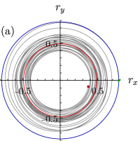
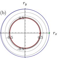
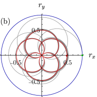
For times much larger than , the effective state’s Bloch vector will oscillate around the composition of the evolution of the preferred subsystem and the dephasing channel i.e. a polar rose, as shown in Figure 3. In cylindrical coordinates, we can write
| (36) | ||||
| (37) | ||||
| (38) |
It is important to underline that such dynamics are obtained assuming large number of particles. This allows us to write the interaction part of the evolution as a dephasing channel (i.e. as a straight line). For finite , a squeezed elliptical trajectory is found. Moreover, the actual trajectory will oscillate around eq. (35) with an amplitude proportional to .
So far, our discussion of the dynamics induced by Hamiltonian (26) centered around the use of the preferential distribution (3). For the non-preferential case, the situation is analogous. Indeed, without interaction, the dynamics will once again follow (30). However, since the depolarization of the state will have a coefficient , it will effectively converge to a point in the axis. In the other hand, for the interacting case, the state’s trajectory will follow the shape of the appropriate rose, but with an increasingly small amplitude, until it also collapses to the axis.
4.2 Ising chain
We now consider an homogeneous and closed Ising spin- chain coupled to a transversal magnetic field, the governing Hamiltonian is the following,
| (39) |
This Hamiltonian is invariant under spin translations, this is, changing indices . We will study the case when the effective initial state is pure,
When all particles participate in the coarse graining (i.e. they have non-zero probabilities in eq. (2)) the only compatible microscopic state is , given that pure states are extremal.
Moreover, observe that the reduced dynamics of one spin is the same for every spin due to the translation symmetry of the Hamiltonian and the permutation symmetry of the initial state. If we denote the reduced density matrix of the -th particle at a time by , this implies that for every , and . Consequently, the effective state at time is simply for any . Therefore, the effective dynamics and the microscopic state are independent of the exact values of , provided that all of them are non-zero ().
Let us now discuss the results. For the system is tractable analytically, see the appendix C for the details. For this case, the reduced dynamics is a non-linear dephasing with rotation around the axis,
| (40) | ||||
with
| (41) |
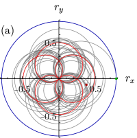
The dynamics is non-linear and does not depend on the total number of spins in the chain. Moreover, it depends only on , see fig. 4; this is expected due to the azimuthal symmetry of the Hamiltonian. Furthermore, both dephasing and rotation depend on , therefore there is a differential rotation apart from the non-linear dephasing, see fig. 5 panel b.
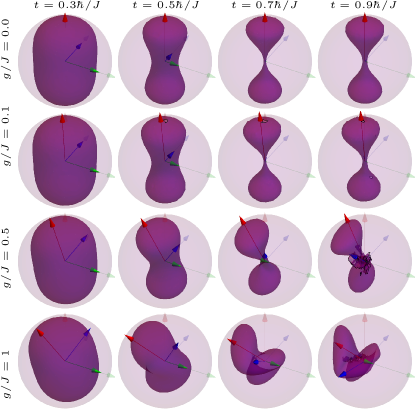
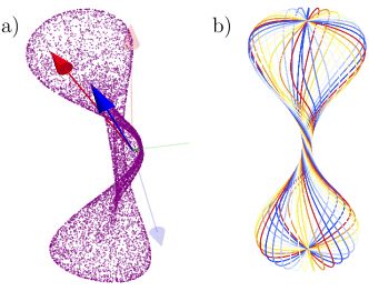
For we performed the calculations numerically with no approximations for initial pure states uniformly distributed. In fig. 4 we plot the results for where it can be observed that the dynamics are more intricate as becomes larger. For and we present a detail of how the central region is twisted in a complicated shape, see fig. 5. The results for (not shown) are quite similar numerically to the ones with when . Moreover, the effective dynamics for the open chain were computed too, and the results are quantitatively similar to the ones of the closed chain (not shown).
As a final note, observe that in this case the non-linearity comes only from the classical correlations between spins (they are always initially aligned). Also we recall that there is not dependency on the distribution defining the coarse graining, but the fact that the probabilities are non-zero for all spins is needed.
5 Linear effective dynamics
In section 3 we presented two examples of microscopic dynamics that give rise to a non-linear, non-Markovian evolution of the effective state. Nevertheless, not all microscopic dynamics will produce such behavior of the effective dynamics. In this section we present some examples of evolutions for which the linearity is preserved under the coarse graining map.
5.1 Channels that act equally on all subsystems
First, let be a quantum channel acting on a two-level system
| (42) |
and let be the density operator that describes a collection of such units. We define as applied locally to each of the subsystems of the -partite system,
| (43) |
according to
| (44) |
for any . By expanding in the basis of tensor products of the Pauli matrices it is a matter of algebra to show that
| (45) |
for any . This means that all channels that act locally and in the same way over all subsystems conserve their linearity under the coarse graining map. What is more, non-factorizable channels that act equally upon all reduced matrices also conserve their linearity.
As a first example, let’s consider dephasing channel. A -qubit total dephasing channel in the direction is
| (46) |
where with . It is not difficult to see that
| (47) |
That is, the total dephasing channel on the microscopic system translates under the coarse graining map as a total dephasing channel over the effective system. The total dephasing channel is an example of a factorizable Pauli component erasing map [19]. A non factorizable PCE map that is also a quantum channel is
| (48) |
with
| (49) |
Note that this acts equally on both reduced density matrices. In fact, it acts as a dephasing channel in the direction upon both subsystems, and so
| (50) |
Although this is an example for two two-level systems, all -qubit quantum channels that satisfy
| (51) |
will give rise to linear effective dynamics.
5.2 A linear non-markovian evolution
Another instance of a microscopic evolution that preserves its linearity under the coarse graining map is the given by the Hamiltonian
| (52) |
Clearly, this is not a mapping that abides by the condition stated by equation (51). However, as we will see, the effective dynamics remain linear with a notable twist: they are non-Markovian. Indeed, using the non-preferential distribution described in equation (3), the microscopic evolution (52) induces the macroscopic dynamics given by
| (53) |
and its effect on the evolution of the effective Bloch vector is described by the following parametric equations:
| (54) | ||||
| (55) | ||||
| (56) |
which represent the parametric equations of a circle in with center at , parallel to the plane, and with radius
The differential equation governing the effective dynamics is
| (57) |
From this differential equation, we can identify the effective Hamiltonian as
| (58) |
where the frequency appearing in the effective Hamiltonian is reduced by half compared to the frequency of the microscopic Hamiltonian. It is worth noting that the equation (57) exhibits singularities at points where the tangent function diverges.
Since the term can be positive or negative, the dynamics are generally non-Markovian. Furthermore, it is straightforward to verify that the corresponding dynamics in (53) do not satisfy the semigroup property:
| (59) |
Thus, coarse-grained quantum dynamics adds to the wide variety of physical systems that exhibit non-Markovianity [20].
6 Discussion an conclusion
We introduced a pragmatic notion of effective dynamics for coarse-grained descriptions of conventional many-body quantum systems. To achieve this, we used the maximum entropy principle to deal with the fact that the effective description emerges from a coarse graining map that irreversibly destroys part of the microscopic information. This method is quite appealing given that no additional information or assumptions are introduced to construct the microscopic state of the system. Next, we assume that the latter undergoes unitary evolution, thus, the system is closed. Remarkably, the emergent dynamics are generally non-linear and depend both on the initial effective state and the probability distribution that defines the coarse graining map.
Additionally, we have proven that such dynamics define non-linear completely positive and trace preserving maps. We believe that this is a beneficial trait given that complete positivity implies positivity, and classical stochastic maps are positive [14]. Moreover, in the absence of quantum correlations, complete positivity is reduced to positivity [21]. This ensures consistency if we consider this framework to investigate the quantum-to-classical transition.
We studied several systems to test the framework, ranging from quantum gates to spin systems. They show explicitly the dependence on the distribution of the coarse graining map and on the initial effective states. However, in the case of the Ising spin chain, its symmetries blind the effective dynamics from the exact values of the distribution, except that they must be greater than zero. It is worth noticing that effective dynamics is not always non-linear, as shown in subsection 5.2. Interestingly, this example is non-linear and non-markovian; thus, closed (and trivially markovian) microscopic dynamics lead to non-markovianity.
We believe that this framework is rich enough to study the emergence of non-linearity in a variety of scenarios, particularly many-body systems, which benefit directly from simplified descriptions. To finalize, several questions arise from this work: under what conditions the emergent non-linearity depends only on the distribution of the coarse graining? Inspired on the Ising spin chain, is it possible to find non-linear dynamics that are independent of the initial state?
Acknowledgments
It is with great pleasure that we thank Fernando de Melo, Raul Vallejo and Hamed Mohammady for their useful comments and suggestions. We acknowledge project VEGA 2/0183/21 (DESCOM) and UNAM-PAPIIT IG101324.
References
- [1] Sebastian Kmiecik, Dominik Gront, Michal Kolinski, Łukasz Wieteska, Aleksandra Badaczewska-Dawid, and Andrzej Kolinski. “Coarse-grained protein models and their applications”. Chemical Reviews116 (2016).
- [2] Paul Busch and Ralf Quadt. “Concepts of coarse graining in quantum mechanics”. International Journal of Theoretical Physics 32, 2261–2269 (1993).
- [3] W.H. Zurek. “Decoherence and the transition from quantum to classical”. Phys. Today 44, 36 (1991). arXiv:quant-ph/0306072.
- [4] Maximilian Schlosshauer. “Decoherence, the measurement problem, and interpretations of quantum mechanics”. Rev. Mod. Phys. 76, 1267–1305 (2005).
- [5] Maximilian Schlosshauer. “Quantum decoherence”. Physics Reports 831, 1–57 (2019).
- [6] Cristhiano Duarte, Gabriel Dias Carvalho, Nadja K. Bernardes, and Fernando de Melo. “Emerging dynamics arising from coarse-grained quantum systems”. Physical Review A96 (2017).
- [7] Pedro Silva Correia, Paola Concha Obando, Raúl O. Vallejos, and Fernando de Melo. “Macro-to-micro quantum mapping and the emergence of nonlinearity”. Physical Review A103 (2021).
- [8] Carlos Pineda, David Davalos, Carlos Viviescas, and Antonio Rosado. “Fuzzy measurements and coarse graining in quantum many-body systems”. Physical Review A104 (2021).
- [9] Raúl O. Vallejos, Pedro Silva Correia, Paola Concha Obando, Nina Machado O’Neill, Alexandre B. Tacla, and Fernando de Melo. “Quantum state inference from coarse-grained descriptions: Analysis and an application to quantum thermodynamics”. Physical Review A106 (2022).
- [10] E. T. Jaynes. “Information theory and statistical mechanics”. Phys. Rev. 106, 620–630 (1957).
- [11] Freeman J. Dyson. “The Threefold Way. Algebraic Structure of Symmetry Groups and Ensembles in Quantum Mechanics”. Journal of Mathematical Physics 3, 1199–1215 (1962). arXiv:https://pubs.aip.org/aip/jmp/article-pdf/3/6/1199/19064331/1199_1_online.pdf.
- [12] Michael A. Nielsen and Isaac L. Chuang. “Quantum computation and quantum information”. Cambridge University Press. (2000).
- [13] Marko Žnidarič, Carlos Pineda, and Ignacio García-Mata. “Non-markovian behavior of small and large complex quantum systems”. Phys. Rev. Lett. 107, 080404 (2011).
- [14] H. P. Breuer and F. Petruccione. “The theory of open quantum systems”. Oxford University Press. Great Clarendon Street (2002).
- [15] David Davalos and Mario Ziman. “Quantum dynamics is not strictly bidivisible”. Phys. Rev. Lett. 130, 080801 (2023).
- [16] Gustavo Montes Cabrera, David Davalos, and Thomas Gorin. “Positivity and complete positivity of differentiable quantum processes”. Physics Letters A 383, 2719–2728 (2019).
- [17] David Davalos, Mario Ziman, and Carlos Pineda. “Divisibility of qubit channels and dynamical maps”. Quantum 3, 144 (2019).
- [18] A Mandilara, J W Clark, and M S Byrd. “Elliptical orbits in the bloch sphere”. Journal of Optics B: Quantum and Semiclassical Optics 7, S277–S282 (2005).
- [19] Jose Alfredo de Leon, Alejandro Fonseca, François Leyvraz, David Davalos, and Carlos Pineda. “Pauli component erasing quantum channels”. Physical Review A106 (2022).
- [20] Li Li, Michael J.W. Hall, and Howard M. Wiseman. “Concepts of quantum non-markovianity: A hierarchy”. Physics Reports 759, 1–51 (2018).
- [21] Alexander S Holevo. “Statistical Structure of Quantum Theory”. Volume 67 of Lecture Notes in Physics Monographs. Springer Berlin Heidelberg. Berlin, Heidelberg (2001).
Appendix A Fuzzy operators
In this section we show the relation between the expected values of a tomographically complete set of observables on the effective Hilbert space and the expected values of what we call fuzzy operators. By remembering that the effective and the microscopic states are related through , we can write
| (60) | ||||
| (61) | ||||
| (62) | ||||
| (63) | ||||
| (64) |
where we have used the fact that swaps are hermitian and the cyclic property of the trace. Additionally, is the observable applied to the th particle. Finally, we can identify the operators as defined in (4) where the following holds,
| (65) |
Appendix B Elliptic CNOT path
Here we show that the interaction term of the CNOT Hamiltonian, , results in an elliptical path for the Bloch vector of the effective state. First, it is easy to show [18] that if we assume that the initial microscopic state is a product state, then the reduced Bloch vectors evolve according to
| (66) | ||||
and
| (67) | ||||
Which correspond to ellipses confined to the and planes. The Bloch vector of the effective state is of course the sum of the Bloch vectors of the two qubits, and thus the effective Bloch vector evolves according to
| (68) |
As it turns out, this is also an ellipse, as in can be written as
| (69) |
Here,
| (70) |
, and
| (71) |
The parameters , , and correspond to the ellipse parameters of the path followed by each reduced system, and they are related to their initial Bloch vectors through
and
Appendix C Ising Model without magnetic field
As mentioned in the main text, to compute the coarse-grained state of the spin chain after the unitary evolution of the microscopic description with , it is enough to compute the reduced density matrix for any spin. To do it, first observe that due to the translation symmetry and the specific form of the initial state , the reduced evolution for each spin is identical. The density matrix of the initial pure state of the spin tagged with , in the computational basis is
and the total density matrix of the microscopic description, also in the computational basis, is
| (72) |
with and the binomial coefficients where and are the numbers of s in and , respectively. We also use the abbreviations and . To derive its evolution it is enough to compute the components and . Now, observe the following, when tracing out all spins except , only operators with the form contribute to , where is a vector indicating the rest of 0s and 1s of the computational basis. Since is an eigenstate of the Hamiltonian, the component remains invariant.
For only operators with the form contribute to the partial trace. Thus, let us investigate their evolution. Observe that both and are eigenvectors of the evolution operator of the spin chain. Therefore, assume that
where is the eigenenergy of . Now, we want to find the relative phase with . To to this it is enough to observe what happens with the nearest neighbors of (spins and ). So we need to investigate the changes in just four configurations: . Starting with , where the spin at the center is and others are its neighbors, changing it to “removes” two terms in the eigenenergy expression of state in favor of two terms, thus
where the left-most spin is the one tagged with and the other spins indicated explicitly are its neighbors. The vector contains the rest of the spins in the computational basis. Putting both kets together we have,
To compute how operators contribute to the partial trace, observe that they appear in the initial density matrix weighted with
where is the number of in (see eq. (72)). Moreover, after tracing out all spins except the one tagged with , there are exactly of such factors for each . Therefore, the total contribution to the operator from the family of operators with the form is
| (73) |
This result, together with the rest of the cases, is summarized in the table 1.
| Operator family | Contribution | Phase |
|---|---|---|
| 1 | ||
| 1 | ||
Appendix D Neglectability of terms in the Dyson series of effective all-to-all interaction
In section 4, chains evolving due to a non uniform external magnetic field in the direction with an all-to-all Ising interaction parallel to the field are considereded. By iteratively itegrating the Liouville–von Neumann equation, a Dyson series, given by equation (32) is obtained. In this series, terms proportional to arise, which are discarded. In this appendix, we show that they are in fact negligible.
By virtue of equation (9), we know that is of the form , and so
| (75) | ||||
Meaning that
| (76) |
The product on the RHS of equation (76) is a product of the components of each subsystem of , which we know to be
| (77) |
Where . Now, as grows, , and if we take of order , then the product
| (78) |
This implies that
| (79) |
which decays exponentially as grows. We conclude that once the coarse graining map is applied, the odd terms in (33) can be approximated by .