SegSTRONG-C: Segmenting Surgical Tools Robustly On Non-adversarial Generated Corruptions – An EndoVis’24 Challenge

Abstract

Accurate segmentation of tools in robot-assisted surgery is critical for machine perception, as it facilitates numerous downstream tasks including augmented reality feedback. While current feed-forward neural network-based methods exhibit excellent segmentation performance under ideal conditions, these models have proven susceptible to even minor corruptions, significantly impairing the model’s performance. This vulnerability is especially problematic in surgical settings where predictions might be used to inform high-stakes decisions.

To better understand model behavior under non-adversarial corruptions, prior work has explored introducing artificial corruptions, like Gaussian noise or contrast perturbation to test set images, to assess model robustness. However, these corruptions are either not photo-realistic or model/task agnostic. Thus, these investigations provide limited insights into model deterioration under realistic surgical corruptions.

To address this limitation, we introduce the SegSTRONG-C challenge that aims to promote the development of algorithms robust to unforeseen but plausible image corruptions of surgery, like smoke, bleeding, and low brightness. We collect and release corruption-free mock endoscopic video sequences for the challenge participants to train their algorithms and benchmark them on video sequences with photo-realistic non-adversarial corruptions for a binary robot tool segmentation task. The training set consists of $11$ corruption-free mock endoscopic surgery sequences, in total of $6600$ frames, and corresponding segmentation masks representing surgical tools. The validation set consists of $3$ video sequences, each with and without corrupted background, in total $3600$ frames. The test set consists of $3$ sequences with non-adversarial corruptions (smoke, bleeding, and low brightness), in total $5400$ frames. This new benchmark will allow us to carefully study neural network robustness to non-adversarial corruptions of surgery, thus constituting an important first step towards more robust models for surgical computer vision. In this paper, we describe the data collection and annotation protocol, baseline evaluations of established segmentation models, and data augmentation-based techniques to enhance model robustness.

Background & Summary

Background:

Robot tool segmentation is a fundamental machine perception task in robot-assisted surgery, enabling numerous downstream tasks. Feed-forward networks (FFN) [1, 2, 3, 4, 5, 6, 7, 8] have dominated this task since deep learning’s emergence and the introduction of public surgical scenes datasets through EndoVis [9, 10] challenges. Methods that achieve state-of-the-art performance on general vision benchmarks [11, 12] also exhibit excellent performance on benchmarks from the surgical domain as the test cases are usually sampled from the same distribution as the training cases and contain minimal corruptions. However, FFNs’ susceptibility to even minor corruptions can significantly impair their performance. This vulnerability is especially critical in high-stakes surgical decisions and poses a significant barrier to clinical translation [13].

Current datasets and data collection/synthesis strategies used to evaluate non-adversarial robustness represented by ImageNet-C [14] are mainly generated synthetically [15]. Thus, their ability to represent corruption likely to occur in surgical scenes remains unknown. To generate test cases that can assess algorithms’ robustness against common complications observed during the surgery, such as smoke, bleeding, and low brightness, Ding et al. [16, 17] utilized the accurate replay functionality of the da Vinci Research Kit(dVRK) [18] to add real-world corruptions to the same trajectory. In this work, we adopt the same data collection pipeline from  [16] and refine it by incorporating the segment anything model (SAM) for more precise and efficient annotations to collect the dataset to assess the algorithms’ robustness against common complications in the surgical scenario.

There are methods proposed to address robustness under non-adversarial corruption with different tactics [15]. Architecture-based tactics address the robustness by developing full architectures [19, 20, 21] or motifs [22, 23, 24, 25]. Data augmentation [26, 27, 28, 29, 30] tactics aim to encourage models to be invariant to non-causal features by increasing the diversity of the training dataset. Optimization-based robustness tactics [31, 32, 33, 34, 35] modify learning objectives to improve resilience to corruption. Auxiliary data(e.g. kinematics in robotics surgery), when available, is used to improve the robustness [17, 16]. However, despite the efforts, a measurable gap remains [15].

We propose the SegSTRONG-C challenge to encourage more attention to the models’ robustness in the healthcare domain and test the robustness under non-adversarial corruptions that commonly happen in the surgical scene to provide more trustworthy assessment and analysis for future directions.

Summary:

With the collected dataset we propose the SegSTRONG-C challenge where participants are challenged to train their algorithms solely on uncorrupted sequences and achieve high performance on corrupted ones for the binary robot tool segmentation task. In this early version of the paper, we present the dataset for the SegSTRONG-C challenge along with its collection and annotation pipeline, the evaluation metrics for the challenge, and a baseline analysis with some segmentation networks and data augmentation methods as baseline models.

Dataset

The dataset consists of mock endoscopic video sequences with corresponding binary segmentation masks for the robot tool segmentation task. We mock the endoscopic scene with two patient-side manipulators (PSMs) and animal tissue backgrounds to ensure a photo-realistic appearance. We manually teleoperate the robot to generate the trajectory in free space. The binary segmentation masks serve as ground truth annotations for surgical tools. The dataset consists of $17$ sequences, collected from different robot and camera configurations and different robot trajectories. Each sequence is collected at $10$ frames per second and consists of $300$ uncorrupted frames for the left camera and $300$ uncorrupted frames for the right camera. We collect all corrupted versions (background, smoke, bleeding, and low brightness) for each sequence under the same configuration and trajectory. We provide $11$ sequences of the dataset with only uncorrupted frames as the train set. We provide $3$ video sequences with uncorrupted frames and corresponding frames with background corruption as the validation set. We use the final 3 sequences with certain corruptions(smoke, bleeding, and low brightness) as the test set. The models submitted by the challenge participants will be tested on this test set consisting of sequences with photo-realistic non-adversarial corruptions. The models will be tested on each corruption separately. As the challenge is currently active, we withhold the release of the test set. Table 1 shows the summary of the dataset. All corrupted versions for the training and validation will be released after the challenge submission. The example images are shown in Figure 1.

Table 1: Dataset summary. "300 + 300" means 300 frames for the left camera and 300 frames for the right camera. "-" means not provided during challenge.

Split	Camera/robot	Trajectory	Non-	Background	Smoke	Bleeding	Low
	configuration id	id	corruption				brightness
Train set	3	1	300 + 300	-	-	-	-
	3	2	300 + 300	-	-	-	-
	4	3	300 + 300	-	-	-	-
	4	4	300 + 300	-	-	-	-
	4	5	300 + 300	-	-	-	-
	5	6	300 + 300	-	-	-	-
	5	7	300 + 300	-	-	-	-
	7	8	300 + 300	-	-	-	-
	7	9	300 + 300	-	-	-	-
	8	10	300 + 300	-	-	-	-
	8	11	300 + 300	-	-	-	-
Validation set	1	12	300 + 300	300 + 300	-	-	-
	1	13	300 + 300	300 + 300	-	-	-
	1	14	300 + 300	300 + 300	-	-	-
Test set	9	15	-	-	300 + 300	300 + 300	300 + 300
	9	16	-	-	300 + 300	300 + 300	300 + 300
	9	17	-	-	300 + 300	300 + 300	300 + 300

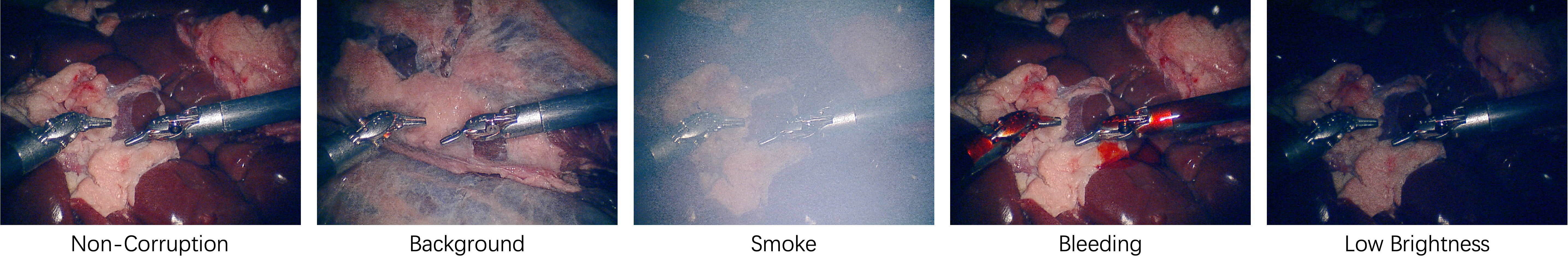
Figure 1: Example images for regular image and non-adversarial corruptions(background, smoke, bleeding, and low brightness.).

Data Collection

The data was acquired in the Robotorium of the Laboratory for Computational Sensing and Robotics (LCSR), Johns Hopkins University by surgical robotics experts familiar with operating the da Vinci robot via dVRK [18]. We use dVRK [18] as our robot platform with the endoscopic camera manufactured by SCHÖLLY and the image process unit manufactured by Ikegami as the perception part. We first adjust the camera/robot configuration and perform calibrations. For each configuration, we collect different trajectories by human operation. For each trajectory, we replay the recorded kinematics to reproduce the trajectory and record video sequences under different scenarios including non-corrupted and corrupted versions with background, smoke, bleeding, and low brightness. To generate non-adversarial corruptions for the same testing samples, we record the robot trajectory, replay the kinematics via dVRK, and manually add corruption for each replay. The background corruption is generated by changing the type of background tissue. The smoke corruption is mimicked by adding artificial fog via a fog machine. The bleeding corruption is mimicked by fake blood. The low brightness corruption is generated by turning down the camera light. The data collection pipeline is shown in the following steps:

• Step1: Camera calibration and hand-eye calibration - We perform a camera calibration to get the intrinsics for the left and right cameras of the stereo and a hand-eye calibration to get the transformation from both cameras to the base frame of both PSM1 and PSM2.

• Step2: Trajectory generation - We use the teleoperation feature of the dVRK to manipulate the PSMs to generate trajectories in free space and record the kinematics of the trajectory.

• Step3: Trajectory replay and recording - We replay the same trajectories and record the videos at 10 fps with the same robot configuration under different scenarios, (1) pure dark background samples for ground truth generation, (2) uncorrupted samples. (3) non-adversarial corrupted samples.

Data annotation

The annotations are generated via a semi-automatic pipeline based on exclusively collected sequences with purely black backgrounds where the only salient areas in the images are the PSMs. We first automatically generate a segmentation mask for the PSMs via the segment anything model (SAM) [36] where the prompts are generated via traditional background extraction algorithm. We select experts who are familiar with the robot and segmentation task to be the annotators to verify and correct the automatically generated annotation. The annotation pipeline can be expressed in the following steps:

• Step 1: Prompt generation - We use a traditional background extraction algorithm to generate rough masks for the foreground PSMs. The rough masks are converted to the prompt points and bounding boxes for SAM.

• Step 2: Automatic generation - We input the prompt with the image to generate a fine mask for the robot tool. The first two steps are fully automatic.

• Step 3: Failure case selection - Human annotators are involved in examining the generated mask from SAM and selecting the failure cases. We had two annotators examining the same sequences and using the union of their selections as the set of failure cases.

• Step 4: Manual correction - The human annotators manually refine the selected failure cases from step 3 via SAM with human prompt input until satisfactory results are achieved. If the annotator had three attempts but did not get satisfactory results, they would draw the contour to annotate this sample manually.

Evaluation

We introduce how we quantitatively evaluate the performance of an algorithm and how we decide the ranking of multiple algorithms that participate in the challenge.

Metrics:

We use dice similarity coefficient (DSC) and normalized surface distance (NSD) averaged from different tolerances for the robot tool for multiple corruptions - low brightness, smoke, and blood. The DSC is a widely used metric in the field of medical image analysis. For a 2D binary class image segmentation task, DSC is defined as

$$DSC=\frac{2TP}{2TP+FP+FN}$$

, where $TP$ is the number of true positive pixels for the class, $FP$ is the number of false positives and $FN$ is the number of false negatives. NSD measures the overlap of two boundaries between the predicted and ground truth segmentation masks. A boundary pixel is counted as overlapping when the closest distance to the other boundary is less or equal to the specified tolerance. NSD for a 2D binary class image segmentation task is defined as:

$$NSD=\frac{\left|S_{A}\cap\mathcal{B}_{B}^{(\tau)}\right|+\left|S_{B}\cap\mathcal{B}_{A}^{(\tau)}\right|}{\left|S_{A}\right|+\left|S_{B}\right|}$$

, where $A$ and $B$ are the masks, $S_{A}$ and $S_{B}$ are boundaries, and $\mathcal{B}_{A}^{(\mathrm{\tau})}$ and $\mathcal{B}_{B}^{(\mathrm{\tau})}$ are the boundary of $A$ and $B$ with an extended border of width tolerance $\tau$. We calculate the average DSC and NSD over images. DSC is the standard metric for segmentation while NSD is complementary to DSC. DSC reveals performance more on the chunk area while NDS focuses on the boundary. We evaluate the performance only on the unseen domain to encourage participants to focus on the algorithm’s robustness.

Ranking:

We rank algorithms with total scores summed over 3 test domains - bleeding, smoke, and low brightness. Each Domain will have two ranks based on the DSC and NSD metrics. For ranking each domain, we will first sort the method based on the metrics over images. Then, we do a pairwise significance test for adjacent methods to test whether they have statistically significant differences in performance. If yes, we rank them according to the order, otherwise they have the same rank. The mean value indicates the overall performance, and the pairwise significance test can justify whether one method has a significant advantage over the other one. We give points in a decreasing arithmetic sequence according to the rank for each test domain. For example, Rank from 1 to 5 and get points from 5 to 1 if there are 5 participants in total. We only test on the unseen corrupted domains as we care about the overall performance of the model on the corrupted domain. Since we have more than one test domain, the summation of points given by rank is a reasonable way to have fair importance for each domain. Using rank and ignoring absolute performance difference is to avoid the result from one specific domain and metric dominating others. Since the goal for the participating team is to develop methods that are robust against all corruptions instead of algorithms achieving dominating performance on one domain but failing to generalize to others, The proposed overall ranking method better suits the goal of the challenge.

Baseline Analysis

In this section, we first briefly introduce the selected segmentation networks and data augmentation methods. Then, we present the testing results of these methods and perform a brief analysis of the baseline results.

Networks

U-Net

: U-Net[2] is originally developed for biomedical image segmentation. The architecture of U-Net consists of two paths: a contracting path and an expansive path. The contracting path is characterized by repeated convolutions and resembles a conventional convolutional network, followed by a rectified linear unit(RELU) and a max pooling operation. On the other hand, the expansive path enhances feature and spatial information through a series of up-convolutions and concatenation of features from the contracting path. Our implementation uses a 4-level vanilla U-Net as the baseline model.

DeepLabV3+

: The most recent version of the DeepLab family is DeepLabV3+ [3]. The architecture is changed to an encoder-decoder structure. The encoder part makes use of atrous separable convolution which separates the convolution process into a Depthwise Convolution and a Pointwise Convolution. Depthwise Convolution applies different kernels to each channel, and Pointwise Convolution combines the outputs across channels. The decoder part combines the low-level features and the upsampled output from the encoder to recover the spatial information by upscaling.

SegFormer

: SegFormer [7] is a semantic segmentation framework that combines a hierarchical transformer encoder with a multi-layer perceptron (MLP) decoder. The hierarchically structured transformer encoder avoids the interpolation of positional codes and outputs multi-scaled features. The lightweight MLP decoder combines both local and global attention to aggregate the multi-layer information.

SETR

: SETR [6] provides an alternative perspective to the encoder-decoder-based FCN architecture. It treats semantic segmentation as a sequence-to-sequence prediction task in which the author splits the image into patches, linearly projects each patch, adds positional embeddings, and feeds the sequence into the transformer encoder. Three different decoders are designed to perform pixel-level segmentation, and we implement all three: (1) Naive upsampling which projects the transformer feature to the dimension of class number and directly upsample to the desired image resolution, (2) Progressive upsampling which alternates convolution and upsampling operations instead of one-step upscaling, and (3) Multi-Level feature aggregation which takes feature representations from $M$ transformer layers uniformly, reshapes and aggregates the feature map top-down, fuses features from all channels and upsamples to the full resolution.

Augmentation

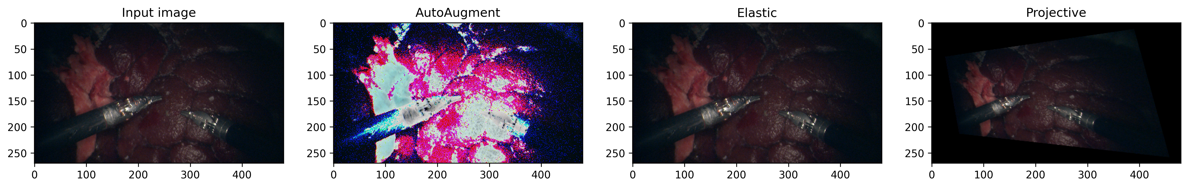
Figure 2: Example image augmentations

AutoAugment

: AutoAugment [30] searches for the best sequence of transformations that improves the performance of a model on a given dataset. We modify the Pytorch implementation of the AutoAugmentPolicy class and choose the policy learned on ImageNet.

Elastic

: Elastic transformation generates displacement vectors for each image pixel based on random offsets. It will transform the image given $\alpha$ and $\beta$, where $\alpha$ controls the strength and $\beta$ controls the smoothness of displacements. We modify the Pytorch implementation of the ElasticTransform class. Let $\alpha_{x}$ and $\alpha_{y}$ be the magnitude of displacements, $\sigma_{x}$ and $\sigma_{y}$ be the smoothness of displacements along $x$ and $y$ axis, and $h$ and $w$ be the height and width of the image. Kernel size along $x$ axis is: $k_{x}=\text{int}(8\sigma_{x}+1)$ thus half of the kernel size is $k_{x\text{\_half}}=\frac{1}{2}(k_{x}-1)$, and the displacement vector $d_{x}$ is first initialized as an array of random numbers between $-1$ and $1$. Each pixel is defined as the Gaussian blur of $d_{x}$ times $\alpha_{x}$ and divided by image height $h$. The 2D Gaussian kernel $h_{x}$ is defined as $h_{x}[m,n]=h_{1}[m]h_{1}[n]^{T}$ where $h_{1}$ is the normalized discrete 1D Gaussian kernel of length $k_{x}$. $d_{x}$, $d_{y}$ is defined as $d_{x}[m,n]=\frac{\alpha_{x}}{h}d_{x}[m,n]*h_{x}[m,n]$, $d_{y}[m,n]=\frac{\alpha_{y}}{w}d_{y}[m,n]*h_{y}[m,n]$. The complete displacement vector field is obtained by concatenating $d_{x}$ and $d_{y}$. The detailed derivations of $h_{1}$, $d_{x}$, and $d_{y}$ are in the equation:

$$h_{1}[m]=\frac{\exp[(-\frac{1}{2}(\frac{-k_{x\text{\_half}}+m}{\sigma_{x}})^{2})]}{\sum_{n=-k_{x\text{\_half}}}^{k_{x\text{\_half}}}\exp[(-\frac{1}{2}(\frac{-k_{x\text{\_half}}+n}{\sigma_{x}})^{2})]}$$

$$d_{x}[m,n]=\frac{\alpha_{x}}{h}\sum_{j=-\infty}^{\infty}\sum_{i=-\infty}^{\infty}d_{x}[i,j]\cdot h_{x}[m-i,n-j]$$

$$d_{y}[m,n]=\frac{\alpha_{y}}{w}\sum_{j=-\infty}^{\infty}\sum_{i=-\infty}^{\infty}d_{y}[i,j]\cdot h_{y}[m-i,n-j]$$

Projective

: Projective transformation transforms the image such that it is viewed from a different viewing perspective with a given probability. We modify the Pytorch implementation of the RandomPerspective class. The four new coordinates of the corners of the image are first randomly generated according to the input distortion scale. In perspective transform, each pixel $(x,y)$ in the original image is mapped to its new coordinate by the formula: $(u_{i},v_{i})=(\frac{ax_{i}+by_{i}+c}{gx_{i}+hy_{i}+1},\frac{dx_{i}+ey_{i}+f}{gx_{i}+hy_{i}+1})$ for $i=0,1,2,3$. In matrix form, it can be written as:

$\begin{bmatrix}x_{0}&y_{0}&1&0&0&0&-x_{0}u_{0}-y_{0}u_{0}\\ x_{1}&y_{1}&1&0&0&0&-x_{1}u_{1}-y_{1}u_{1}\\ x_{2}&y_{2}&1&0&0&0&-x_{2}u_{2}-y_{2}u_{2}\\ x_{3}&y_{3}&1&0&0&0&-x_{3}u_{3}-y_{3}u_{3}\\ 0&0&0&x_{0}&y_{0}&1&-x_{0}v_{0}-y_{0}v_{0}\\ 0&0&0&x_{1}&y_{1}&1&-x_{1}v_{1}-y_{1}v_{1}\\ 0&0&0&x_{2}&y_{2}&1&-x_{2}v_{2}-y_{2}v_{2}\\ 0&0&0&x_{3}&y_{3}&1&-x_{3}v_{3}-y_{3}v_{3}\end{bmatrix}\cdot\begin{bmatrix}a\\ b\\ c\\ d\\ e\\ f\\ g\\ h\end{bmatrix}=\begin{bmatrix}u_{0}\\ u_{1}\\ u_{2}\\ u_{3}\\ v_{0}\\ v_{1}\\ v_{2}\\ v_{3}\end{bmatrix}$

Solve this system to obtain the least-square solution for the coefficients, and map each pixel to its new position by the perspective transformation formula.

Results

We evaluate the performance of baseline models with and without data augmentation across different domains. While all models show reasonable accuracy under regular conditions, their effectiveness substantially deteriorates when tested in shifted domains such as in the presence of bleeding, low brightness, and smoke. The data augmentations applied, including AutoAugment, elastic, and projective transformations, generally failed to improve model performance in these domains. Notably, UNet combined with AutoAugment showed a marginal improvement under smoke conditions but this improvement is inconsistent across all domains. As shown in Figure 3, under regular conditions, the models adequately segmented tools from the background, but struggled in areas with appearance change and subtle contrast changes. Failures are predominantly under bleeding conditions due to the appearance (color) change of the shaft, leading to incorrect segmentation of the shaft. Under low brightness conditions, the darker the region is, the more likely a failure in segmentation will occur. The pervasive false positives under smoke conditions indicate that the models interpret the bright regions (smoke) as the foreground. These results suggest that all baseline models are highly dependent on adequate targets’ saliency to successfully distinguish between the tools and the background. They are also sensitive to any appearance change for the tool (bleeding) and background (smoke).

Table 2: Experiment results of baseline models across different domains.

Models	NSD			DSC
	Bleeding	Smoke	Low Brightness	Bleeding	Smoke	Low Brightness
DeepLabv3 [3]	0.5629	0.4637	0.4000	0.6896	0.6538	0.5352
Segformer [7]	0.5133	0.5266	0.4194	0.6802	0.6906	0.6145
SETR_PUP [6]	0.2531	0.3354	0.2599	0.4717	0.5848	0.4053
SETR_MLA [6]	0.2798	0.3374	0.1571	0.5358	0.6206	0.3385
SETR_Naive [6]	0.3312	0.4409	0.0092	0.5064	0.6657	0.0275
UNet [2]	0.5677	0.5084	0.4390	0.7052	0.6603	0.5750
UNet [2] + AutoAugment [30]	0.6654	0.8152	0.5344	0.7910	0.8895	0.6965
UNet [2] + Elastic	0.5622	0.5207	0.3931	0.6910	0.6583	0.5190
UNet [2] + Projective	0.5661	0.5702	0.4265	0.6903	0.6978	0.5792
SETR [6] + AutoAugment [30]	0.1172	0.0910	0.0773	0.1918	0.2157	0.0934
SETR [6] + Elastic	0.2836	0.3363	0.1654	0.5350	0.6192	0.3472
SETR [6]+ Projective	0.2240	0.3055	0.0552	0.4168	0.5766	0.1447

Conclusion

We present the SegSTRONG-C challenge, aiming to assess algorithms’ robustness to unforeseen yet plausible complications in surgical scenarios. To generate non-adversarial corruptions we use and refine the data collection and annotation pipeline from CaRTS [16] and collect 17 sequences for training and evaluation. We use DSC and NSD as quantitative metrics to evaluate algorithms’ performance on the testing set and propose a balanced ranking method to alleviate the influence of extreme performance on a single domain while emphasizing the statistical significance during ranking. The baseline analysis provides baseline performance for participants to refer to while providing a basic insight that the models’ success relies on adequate saliency and that all models are sensitive to appearance change.

Acknowledgement:

This Challenge is supported by the collaborative research agreement with the MultiScale Medical Robotics Center at The Chinese University of Hong Kong, Intuitive Surgical Inc, and Johns Hopkins University internal funds.

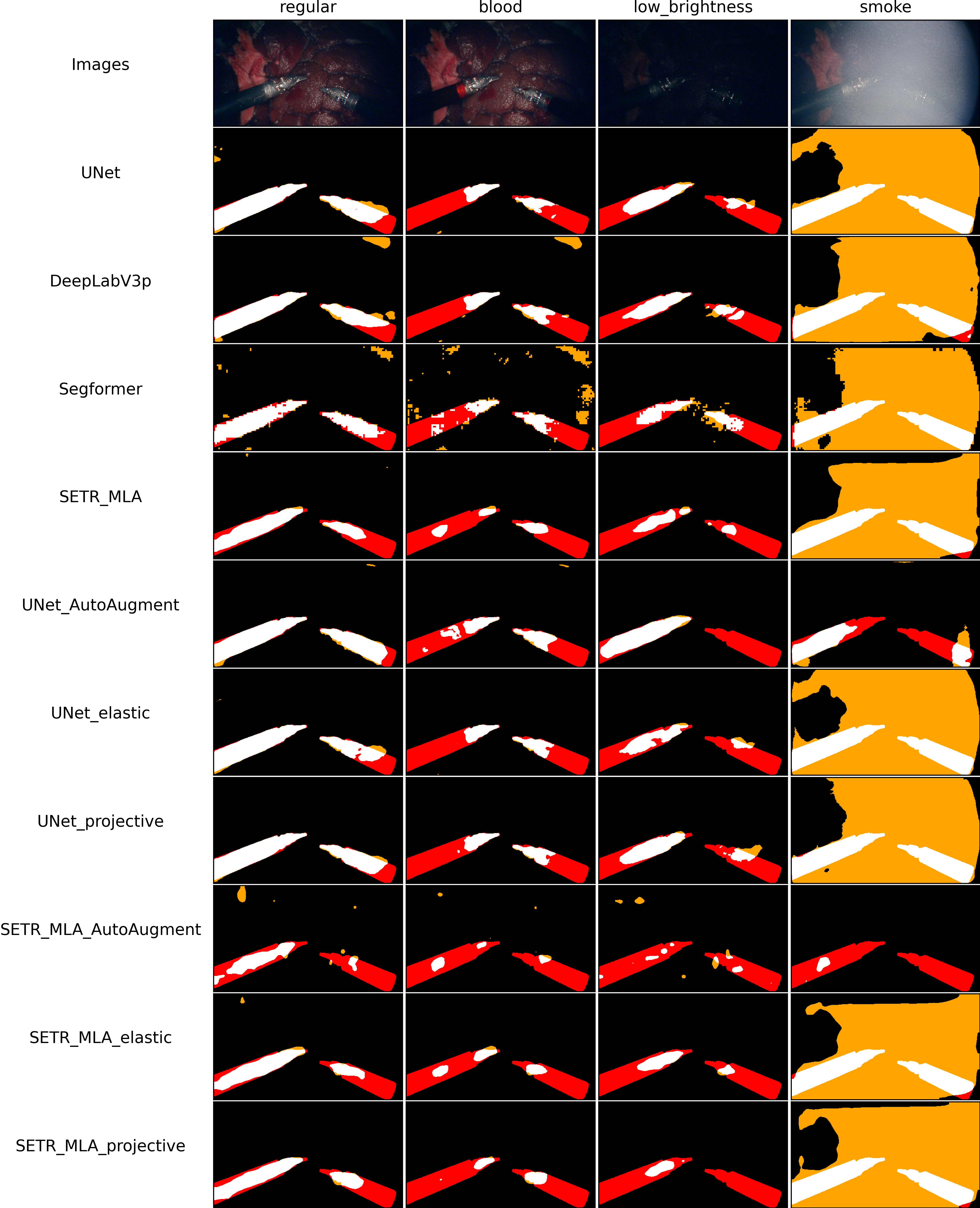
Figure 3: Baseline results. The white area means true positive, the red area means false negative, and the orange area means false positive.

References

- [1] Long, J., Shelhamer, E. & Darrell, T. Fully convolutional networks for semantic segmentation. In Proceedings of the IEEE conference on computer vision and pattern recognition, 3431–3440 (2015).
- [2] Ronneberger, O., Fischer, P. & Brox, T. U-net: Convolutional networks for biomedical image segmentation. In Medical Image Computing and Computer-Assisted Intervention–MICCAI 2015: 18th International Conference, Munich, Germany, October 5-9, 2015, Proceedings, Part III 18, 234–241 (Springer, 2015).
- [3] Chen, L.-C., Zhu, Y., Papandreou, G., Schroff, F. & Adam, H. Encoder-decoder with atrous separable convolution for semantic image segmentation. In Proceedings of the European conference on computer vision (ECCV), 801–818 (2018).
- [4] Zhao, H., Shi, J., Qi, X., Wang, X. & Jia, J. Pyramid scene parsing network. In Proceedings of the IEEE conference on computer vision and pattern recognition, 2881–2890 (2017).
- [5] Seenivasan, L., Mitheran, S., Islam, M. & Ren, H. Global-reasoned multi-task learning model for surgical scene understanding. \JournalTitleIEEE Robotics and Automation Letters 7, 3858–3865 (2022).
- [6] Zheng, S. et al. Rethinking semantic segmentation from a sequence-to-sequence perspective with transformers. In Proceedings of the IEEE/CVF conference on computer vision and pattern recognition, 6881–6890 (2021).
- [7] Xie, E. et al. Segformer: Simple and efficient design for semantic segmentation with transformers. \JournalTitleAdvances in Neural Information Processing Systems 34, 12077–12090 (2021).
- [8] Cheng, B., Misra, I., Schwing, A. G., Kirillov, A. & Girdhar, R. Masked-attention mask transformer for universal image segmentation. In Proceedings of the IEEE/CVF conference on computer vision and pattern recognition, 1290–1299 (2022).
- [9] Allan, M. et al. 2018 robotic scene segmentation challenge. \JournalTitlearXiv preprint arXiv:2001.11190 (2020).
- [10] Allan, M. et al. 2017 robotic instrument segmentation challenge. \JournalTitlearXiv preprint arXiv:1902.06426 (2019).
- [11] Everingham, M., Van Gool, L., Williams, C. K., Winn, J. & Zisserman, A. The pascal visual object classes (voc) challenge. \JournalTitleInternational journal of computer vision 88, 303–338 (2010).
- [12] Zhou, B. et al. Semantic understanding of scenes through the ade20k dataset. \JournalTitleInternational Journal of Computer Vision 127, 302–321 (2019).
- [13] Maier-Hein, L. et al. Surgical data science–from concepts toward clinical translation. \JournalTitleMedical image analysis 76, 102306 (2022).
- [14] Hendrycks, D. & Dietterich, T. Benchmarking neural network robustness to common corruptions and perturbations. \JournalTitlearXiv preprint arXiv:1903.12261 (2019).
- [15] Drenkow, N., Sani, N., Shpitser, I. & Unberath, M. A systematic review of robustness in deep learning for computer vision: Mind the gap? \JournalTitlearXiv preprint arXiv:2112.00639 (2021).
- [16] Ding, H., Zhang, J., Kazanzides, P., Wu, J. Y. & Unberath, M. Carts: Causality-driven robot tool segmentation from vision and kinematics data. In International conference on medical image computing and computer-assisted intervention, 387–398 (Springer, 2022).
- [17] Colleoni, E., Edwards, P. & Stoyanov, D. Synthetic and real inputs for tool segmentation in robotic surgery. In International Conference on Medical Image Computing and Computer-Assisted Intervention, 700–710 (Springer, 2020).
- [18] Kazanzides, P. et al. An open-source research kit for the da vinci® surgical system. In 2014 IEEE international conference on robotics and automation (ICRA), 6434–6439 (IEEE, 2014).
- [19] Costante, G., Mancini, M., Valigi, P. & Ciarfuglia, T. A. Exploring Representation Learning With CNNs for Frame-to-Frame Ego-Motion Estimation. \JournalTitleIEEE Rob. Autom. Lett. 1, 18–25, 10.1109/LRA.2015.2505717 (2015).
- [20] Liu, X. et al. How does noise help robustness? explanation and exploration under the neural sde framework. In Proceedings of the IEEE/CVF conference on computer vision and pattern recognition, 282–290 (2020).
- [21] Subramaniam, A., Balasubramanian, P. & Mittal, A. Ncc-net: Normalized cross correlation based deep matcher with robustness to illumination variations. In 2018 IEEE Winter Conference on Applications of Computer Vision (WACV), 1944–1953 (IEEE, 2018).
- [22] Agostinelli, F., Anderson, M. R. & Lee, H. Adaptive multi-column deep neural networks with application to robust image denoising. \JournalTitleAdvances in neural information processing systems 26 (2013).
- [23] Aspandi, D., Martinez, O., Sukno, F. & Binefa, X. Robust facial alignment with internal denoising auto-encoder. In 2019 16th Conference on Computer and Robot Vision (CRV), 143–150 (IEEE, 2019).
- [24] Bastidas, A. A. & Tang, H. Channel attention networks. In Proceedings of the IEEE/CVF conference on computer vision and pattern recognition workshops, 0–0 (2019).
- [25] Dapello, J. et al. Simulating a primary visual cortex at the front of cnns improves robustness to image perturbations. \JournalTitleAdvances in Neural Information Processing Systems 33, 13073–13087 (2020).
- [26] Geirhos, R. et al. Generalisation in humans and deep neural networks. \JournalTitleAdvances in neural information processing systems 31 (2018).
- [27] Huang, Y. et al. Some investigations on robustness of deep learning in limited angle tomography. In Medical Image Computing and Computer Assisted Intervention–MICCAI 2018: 21st International Conference, Granada, Spain, September 16-20, 2018, Proceedings, Part I, 145–153 (Springer, 2018).
- [28] Laugros, A., Caplier, A. & Ospici, M. Are adversarial robustness and common perturbation robustness independant attributes? In Proceedings of the IEEE/CVF International Conference on Computer Vision Workshops, 0–0 (2019).
- [29] Zhang, H., Cisse, M., Dauphin, Y. N. & Lopez-Paz, D. mixup: Beyond empirical risk minimization. \JournalTitlearXiv preprint arXiv:1710.09412 (2017).
- [30] Cubuk, E. D., Zoph, B., Mane, D., Vasudevan, V. & Le, Q. V. Autoaugment: Learning augmentation strategies from data. In Proceedings of the IEEE/CVF conference on computer vision and pattern recognition, 113–123 (2019).
- [31] Madry, A., Makelov, A., Schmidt, L., Tsipras, D. & Vladu, A. Towards deep learning models resistant to adversarial attacks. \JournalTitlearXiv preprint arXiv:1706.06083 (2017).
- [32] Rusak, E. et al. A simple way to make neural networks robust against diverse image corruptions. In Computer Vision–ECCV 2020: 16th European Conference, Glasgow, UK, August 23–28, 2020, Proceedings, Part III 16, 53–69 (Springer, 2020).
- [33] Wang, H., Ge, S., Lipton, Z. & Xing, E. P. Learning robust global representations by penalizing local predictive power. \JournalTitleAdvances in Neural Information Processing Systems 32 (2019).
- [34] Zhao, L., Liu, T., Peng, X. & Metaxas, D. Maximum-entropy adversarial data augmentation for improved generalization and robustness. \JournalTitleAdvances in Neural Information Processing Systems 33, 14435–14447 (2020).
- [35] Yang, T., Zhu, S. & Chen, C. Gradaug: A new regularization method for deep neural networks. \JournalTitleAdvances in neural information processing systems 33, 14207–14218 (2020).
- [36] Kirillov, A. et al. Segment anything. \JournalTitlearXiv preprint arXiv:2304.02643 (2023).