footinclude=false \KOMAoptionsheadsepline=true \KOMAoptionsDIV=12 \recalctypearea\AfterCalculatingTypearea \recalctypearea
An implementation of -FEM for the fractional Laplacian
Abstract
We consider the discretization of the -integral Dirichlet fractional Laplacian by -finite elements. We present quadrature schemes to set up the stiffness matrix and load vector that preserve the exponential convergence of -FEM on geometric meshes. The schemes are based on Gauss-Jacobi and Gauss-Legendre rules. We show that taking a number of quadrature points slightly exceeding the polynomial degree is enough to preserve root exponential convergence. The total number of algebraic operations to set up the system is , where is the problem size. Numerical example illustrate the analysis. We also extend our analysis to the fractional Laplacian in higher dimensions for -finite element spaces based on shape regular meshes.
1 Introduction
Fractional differential equations have become an important modelling tool, which sparked significant research in analysis and design and analysis of numerical methods, see, e.g., [BV16] and, for numerical methods, [BBN+18, BLN20, LPG+20, DDG+20, JZ23, Kar19, ZWSK24] and references therein.
We consider the fractional differential equation
| (1.1a) | ||||
| (1.1b) | ||||
where , and is analytic in . Here, the operator is the Dirichlet integral fractional Laplacian, defined in (2.1) below. Among the discretization techniques, methods like the -finite element method (FEM) stand out as they achieve exponential convergence, [BFM+23, FMMS23], so that significantly fewer degrees of freedom are required to achieve the same accuracy compared to fixed order methods such as the classical -FEM. This is particularly interesting for non-local problems such as fractional PDEs since there the stiffness matrices are fully populated with corresponding high memory requirements and high complexity to set up the matrices.
In fact, [BFM+23] considers -FEM approximations on suitably designed geometric meshes in one space dimension and shows, for the -FEM approximation to the solution of (1.1), the energy-norm error estimate
| (1.2) |
where are constants independent of the problem size . Such exponential convergence results generalize to higher dimensions, e.g., in two space dimensions [FMMS23] asserts a similar convergence estimate where the square root in the exponent is replaced by .
The exponential convergence in [BFM+23, FMMS23] is asserted ignoring variational crimes, in particular, it is shown under the assumption that is the exact -finite element Galerkin approximation to . However, a practical realization of the Galerkin method (2.2) requires the evaluation of singular integrals by numerical quadrature. In the present work we develop and analyze quadrature schemes that preserve the exponential convergence (1.2). The quadratures are based on Gauss-Legendre and Gauss-Jacobi rules, and the analysis is performed in the framework of the First Strang Lemma. The key observation is that the hyper-singular integrand can be transformed such that singularities are aligned with coordinate axes, which allows for efficient treatment with Gauss-Jacobi rules.
The issue of evaluating singular integrals has already appeared in the context of boundary element methods (BEMs), [SS11]. For the kernels of BEM-operators arising from second order elliptic boundary value problems, regularizing transformations for the singular integrals have been devised that fully remove the singularity so that standard quadrature techniques can be brought to bear and a full quadrature error analysis is available, [SS11, Chap. 5]. For certain meshes with structure even the high order stiffness matrices of -BEM can be computed explicitly, [Mai95, HMS96]. Generalizing the quadrature techniques described in [SS11, Chap. 5] the works [CvPS11, CS12, CR13, CvPS15] present and analyze regularizing transformations for a class of integrands that includes products of analytic/Gevrey-regular functions and singular functions; computationally, an essential point of these transformations is that they lead to the use of products of Gauss-Legendre and -quadrature or Gauss-Jacobi quadrature. Using similar transformations (in 1d) and building on these works (for ), our analysis considers the specific case of -FEM for the fractional Laplacian, explicitly works out the dependence on the polynomial degree of the ansatz space, and asserts exponential convergence of the fully discrete method. The work to set up the stiffness matrix is algebraic in the problem size.
Implementations of the spectral fractional Laplacian have been proposed in the literature. Low order (for ) Galerkin methods include [ABB17, AG18, FB23] and typically exploit that a specific choice of basis is made in contrast to the present quadrature-based approach. Especially for fractional differential equations, spectral and spectral element methods are available in the literature, see, e.g., [Kar19, LZZ19, SS19, ZK13, ZWSK24, LPG+20, MS18, CSW16] and references therein. The quadrature techniques employed in the present work on shape regular meshes are closely related to those presented independently in [MS18]. Compared to these works, an important novel aspect of the present work is the full quadrature error analysis that rigorously establishes that taking quadrature points ( denoting the employed polynomial degree) is sufficient to retain the exponential convergence of -FEM.
In the present article, we consider the case in great detail to make key concepts appear clearly. Extensions to are possible, but come with additional (technical) difficulties. We present an analysis for for shape regular meshes based on the regularizing transformations of [CS12] in Section 6. We hasten to add that exponential convergence (both in terms of error versus number of degrees of freedom and error versus computational work) of -FEM in requires anisotropic elements with large aspect ratio, [FMMS23]. A quadrature error analysis for meshes including anisotropic elements is the topic of a forthcoming work.
The present article is structured as follows: In Section 2, we introduce our model problem and formulate the main result, exponential convergence of -FEM in the presence of quadrature, in Theorem 2.4. Section 3 specifies the Gaussian quadrature rules and the resulting approximation of the bilinear and linear forms in the weak formulation of the model problem. Section 3.1 shows stability of the method under quadrature. Section 4 provides the proofs of our main results using the First Strang Lemma, while the consistency analysis is postponed to Section 5. Section 6 extends the -analysis to higher dimensions for shape regular meshes based on the quadrature techniques developed in [CvPS11, CS12].
Finally, Section 7 provides numerical examples illustrating the performance of the quadrature scheme.
2 Main Results
For , we consider the integral fractional Laplacian defined for univariate functions pointwise as the principal value singular integral
| (2.1) |
where denotes the Gamma function.
Appropriate function spaces for fractional differential equations are fractional Sobolev spaces, defined for and any open set by means of the Aronstein-Slobodeckij seminorm
In order to incorporate the exterior Dirichlet condition, we define and introduce the space with norm
With the exception of Section 6 the domain always denotes the bounded open interval from our model problem (1.1); in Section 6, we will consider polyhedral . We will use the fact that the norm and the seminorm are equivalent on , [McL00]. The weak form of the fractional PDE (1.1) reads: find such that
| (2.2) |
for all . Since is continuous and coercive on , (2.2) is uniquely solvable by the Lax-Milgram Lemma, see [AB17, Sec. 2.1].
For the discretization of the weak formulation, we employ piecewise polynomials on shape regular meshes.
Definition 2.1 (Shape regular meshes and spline spaces).
For an interval , we denote its length by . For a bounded interval let the points determine the mesh . The mesh is said to be -shape regular, if
| (2.3) |
Based on , we define finite dimensional spline spaces by
Here, denotes the space of all polynomials with maximal degree on .
The standard basis for is given by
| (2.4) |
where are the hat functions associated with the interior nodes and with element bubble functions . For an element with length , the element bubble functions are given by
| (2.5) |
where is the -th Legendre polynomial.
The -FEM approximation is given by Galerkin discretization of (2.2): Find such that
| (2.6) |
For a given basis of , finding the solution is equivalent to setting up and solving the linear system
| (2.7) |
where with and with . Setting up the linear system requires evaluating the bilinear form for all pairs of basis functions, which means calculating (singular) double integrals. Computing the linear form for all basis functions leads to a routine problem of calculating integrals involving .
Our main convergence results are formulated for a specific kind of shape regular meshes, so-called geometric meshes, defined in the following Definition 2.2. However, we emphasize that the analysis of the consistency errors of the bilinear and linear forms in Chapter 5 hold for arbitrary shape regular meshes.
Definition 2.2 (Geometric mesh and basis of the spline space ).
Given a grading factor and a number of layers, the geometric mesh with elements is defined by the nodes
We note that and that is shape regular with .
The basis for is taken as the basis of Definition 2.1 for the mesh .
In [BFM+23] the following exponential convergence results for the energy norm error between the solution in (2.2) and its -FEM approximation from (2.6) on geometric meshes is shown:
Proposition 2.3 ([BFM+23]).
Let be a geometric mesh on the interval with grading factor and layers of refinement towards the boundary points. Let the data be analytic in . Let solve (2.6) with and solve (2.2). Then, there are , and for all there is such that for all and there holds
| (2.8) |
The choice leads to convergence , where is the dimension of and are constants independent of .
In practice, it is not possible to set up the linear system of equations corresponding to (2.6) exactly due to the presence of the kernel function . To implement the -FEM method, we therefore have to work with computable numerical approximations and of the bilinear form and the right-hand side , respectively. The fully discrete problem then reads: Find such that
| (2.9) |
In Section 3 below, we specify the approximations and based on (weighted) Gaussian quadrature rules with points. Our main result formulated in the following states that the exponential convergence rate of to the solution is still preserved.
Theorem 2.4 (Exponential convergence including quadrature).
Let be a geometric mesh on the interval with grading factor and layers of refinement towards the boundary points. Let be analytic in , denote by the solution to (2.2) and by the solution to (2.9) with , where and are defined in (3.13) and (3), respectively. The index indicates the number of quadrature points that is used per integral and element.
There are constants , and, for each a constant ( depending on , , and ) such that for any , , there holds
| (2.10) |
For and there holds in terms of the problem size for some independent of and
| (2.11) |
For and the basis from Definition 2.2, the number of algebraic operations to set up the linear system corresponding to (2.7) is .
3 Quadrature approximations
Throughout this section, we consider -shape regular meshes . We start with some general definitions and notations. denotes the reference element and, for each element , we define the affine element map by
| (3.1) |
With a slight abuse of notation, we will naturally extend to an affine function when needed. For a function defined on , we write for its pullback to the reference element
| (3.2) |
Our approximations to and are based on the following (weighted) Gaussian quadrature rules.
Let be a positive, integrable weight function. Then, we approximate
where are the Gaussian quadrature nodes (zeros of orthogonal polynomials w.r.t. the -weighted -inner product) and with the -th Lagrange interpolation polynomials associated with the quadrature nodes .
For , we write (Gauss-Legendre quadrature) for the quadrature rule. For integrands with singularities at the boundaries, we take and write (Gauss-Jacobi quadrature). For multivariate functions , we will indicate by the subscript , the variable to which the quadrature rule is applied.
We start by deriving an approximation to the right-hand side in (2.6). Dividing the integration domain into the elements , transforming them to the reference element , and using Gauss-Legendre quadrature for each integral defines the linear form for by
| (3.3) |
The approximation of the bilinear form is more involved since we have to deal with hyper-singular double integrals. Using symmetry and dividing the integration domain into the elements and the complementary set leads to
| (3.4) |
where, for arbitrary sets , the symbol denotes
| (3.5) |
The integral over can be integrated explicitly. All the other integrals have to be transformed to a reference square and then approximated by a suitable quadrature rule, which leads to four cases.
Identical elements ():
We transform the double integral to the reference square and divide this integration domain into the triangles and . As the integrand is invariant under the transformation , we notice that both integrals are the same. Employing the Duffy transformation, i.e., , leads to
| (3.6) |
We note that after the separation of the weight function, the integrand in (3) is a polynomial since only removable singularities are left.
Remark 3.1.
Our choice of the Gauss-Jacobi weight function is not the only possible option, as, e.g., one could cancel out one power of in the first equality in (3). However, our choice is optimal in the sense that it decreases the polynomial degree of the integrand as much as possible.
Adjacent elements ( with ):
Without loss of generality, we may assume that is the left neighbor of , otherwise and change their roles. Then, the element maps transform the singularity at to the point in the reference square. With an additional transformation we are now in a similar setting as in the previous case. The integral can be split into integrals over and and employing the Duffy transformation on (for we take ) leads to
| (3.7) |
The singularities appear only in one variable in each integral, for which we employ Gauss-Jacobi quadrature, while in the other variable Gauss-Legendre quadrature is sufficient. This gives the approximation
| (3.8) | ||||
| (3.9) |
Separated elements ():
This time, the integrand is not singular. Therefore, one can directly transform the double integral to the reference square and employ tensor product Gauss-Legendre quadrature, which produces as the approximation of the expression
where denotes the Euclidean distance between the elements and .
Complement part ():
The inner integral over can be calculated explicitly exploiting that the functions vanish outside of . The outer integral can be transformed to the reference element , which gives
| (3.10) |
If is an interior element, i.e., , we employ Gauss-Legendre quadrature
For , we set
| (3.11) |
and for
| (3.12) |
Now, having defined for all cases of integrals , we obtain the approximated bilinear form as
| (3.13) |
3.1 Stability of the quadrature rule
Positivity of the kernel function and the Gauss-Legendre/Gauss-Jacobi weights as well as exactness of the Gauss-Legendre/Gauss-Jacobi quadrature allow us to prove the following stability result:
Lemma 3.2.
Let be a -shape regular mesh. Then, the following holds:
-
(i)
For all and all , we have .
-
(ii)
Let and . Then implies . In particular, the stiffness matrix in (2.7) is symmetric positive definite.
Furthermore, there is depending only on and such that for all the following assertions hold:
-
(iii)
(Identical elements) For and : .
-
(iv)
(Adjacent elements) For and with and : .
-
(v)
(Separated elements) For and with : .
Proof.
Proof of (i): This follows from the positivity of the kernel and the Gauss-Legendre/Gauss-Jacobi weights.
Proof of (ii): From (i), we get for with
Hence, for each so that is constant on each element. By continuity of , it is constant on , and the boundary conditions then imply .
Proof of (iii): For , the univariate Gauss-Jacobi quadrature in (3) is exact for polynomials of degree . Inspection of (3) shows that the argument is the square of a polynomial of degree in each variable.
Proof of (iv): For , the univariate Gauss-Jacobi quadratures in (3.8) are exact for polynomials of degree . We study the cases and separately, starting with . We only consider the first term in (3.8), the other one being handled analogously. Let . For the pull-backs , to the reference element of the functions , , we get by continuity of at that . Hence,
is a polynomial of degree in and of degree in . Using the positivity of the quadrature weights and the exactness of the quadrature rules ( is a polynomial of degree in each variable)
where we used in the last inequality that . We conclude in view of (3)
where depends only the shape regularity constant and . The case leads to two terms of the form (3.11) or (3.12). One term can always be analyzed in similar fashion as above and the other one can be treated as in the following case (v).
Proof of (v): This is handled similarly to the case of adjacent elements in (iv). We consider only the case , the case is handled similarly.
With , as above and using that polynomials of degree are integrated exactly for we estimate
for a that depends solely on the shape regularity constant and . ∎
Remark 3.3.
The proof shows that the condition for the case of adjacent elements could be weakened in that points suffice in one variable whereas point should be used in the other one.
Corollary 3.4.
Let be a -shape regular mesh. There is depending only on and such that for
| (3.14) |
Proof.
Remark 3.5.
4 Proof of Theorem 2.4
The proof is based on the classical Strang Lemma, see, e.g., [Bra07, Chap. 3]. In the present setting, it takes the following form:
Lemma 4.1 (First Strang Lemma).
Lemma 4.1 indicates that we have to show lower bounds for the coercivity of as well as derive bounds for the consistency errors and . This is the subject of the following two lemmas, whose proofs are postponed to Section 5.
Lemma 4.2 (Consistency error for ).
Let be analytic in , and let be a -shape regular mesh. Let and let its approximation be defined by (3). Then, there exists a constant depending only on such that
| (4.2) |
where is a constant that depends only on and .
Lemma 4.3 (Consistency error for ).
As pointed out in Remark 3.5, the consistency error allows one to infer uniform coercivity by a perturbation argument:
Lemma 4.4 (Uniform coercivity).
Let the assumptions of Lemma 4.3 hold. Then, there are constants depending only on the shape regularity constant and such that for there holds
| (4.4) |
Proof.
The coercivity of , the triangle inequality and Lemma 4.3 applied with give
As the second term on the right-hand side tends to zero for , we may ensure for with large enough constants that
| (4.5) |
so that coercivity of follows with coercivity constant . To give more details: we note that , can be chosen independently of and as
-
•
,
-
•
,
-
•
,
which directly gives (4.5). ∎
Proof of Theorem 2.4.
Proof of (2.10): Under the assumptions made, we can apply the stability result Corollary 3.4 with noting that . Hence, for , we can use the First Strang Lemma to estimate
| (4.6) |
Taking as the -FEM approximation of (2.6) for the space , we get from Proposition 2.3 for the first term
| (4.7) |
Lemma 4.3 and the a priori estimate lead to
| (4.8) |
Finally, Lemma 4.2 provides
| (4.9) |
This proves the convergence result (2.10).
Proof of the complexity estimate: We are left to show that, for and the basis from Definition 2.2, the number of algebraic operations to set up the linear system is , where with and with . The key to the proof is that the evaluation of the shape functions at the quadrature points always happens on the reference element and therefore can be precomputed. This precomputation can be realized in operations using three-term recurrence relations by noting that the integrated Legendre polynomials are orthogonal polynomials (see, e.g., [KS05, (A.3), (A.9)]).
We recall that the support of the basis functions consists of two mesh elements for and one for . Therefore, in the definition of the approximated bilinear form
most of the summands are zero and only are left to calculate. Before we derive the stated complexity bound, we show that a direct implementation is not enough to achieve .
Direct implementation: In terms of computational effort, the evaluation of the stiffness matrix dominates the computation of the load vector (which is of order by the same reasoning as below). For the stiffness matrix, a naive implementation contains nested loops (starting from the outer loops) of
-
•
2 loops over the basis functions (thus complexity ) with evaluation of quadrature formulas of the type and ;
-
•
evaluation of each and : 2 loops over the quadrature points with complexity .
In total this leads to a complexity of , since . We now show that the complexity of setting up the stiffness matrix and therefore the overall complexity, can actually be reduced from to .
Step 1 (blockwise assembly): We assemble the stiffness matrix blockwise. Therefore, for subsets of basis functions , we introduce the notation for a matrix block.
As , we have . The block has entries (as ) that can each be calculated in operations. Similarly, the blocks and have entries ( as ), which can be each calculated in operations. Thus, the total complexity for the calculation of these three blocks is operations. It thus remains to treat the block .
Step 2 (treatment of ): Let be a pair of elements. We distinguish three cases: the pairs of adjacent elements, the coinciding pairs , and the well-separated pairs. For the first two cases of adjacent pairs or identical pairs, one has to consider combinations of basis functions so that the total complexity for this case is , which is the desired complexity.
Therefore, let be separated, i.e., and be fixed. For this case, the bilinear form simplifies to
| (4.10) |
where . The key observation is that the vectors and can be precomputed in operations using recurrence relations since and are the integrated Legendre polynomials on the reference element and therefore independent of and . Thus, we can compute the products in (4) as: For all pairs of separated elements , and all , compute the vectors
-
•
in ;
-
•
then, loop over all basis functions and compute the scalar product in .
This leads to a total complexity of , which finishes the proof.
∎
5 Consistency errors
We start with a well-known basic error estimate for Gaussian quadrature. Recall that
with and that the numerical integration is exact for . Thus, for an arbitrary polynomial we get (using also the positivity of the weights )
which gives the best approximation estimate
| (5.1) |
By tensorization, this result for univariate Gaussian quadrature can be extended to the -case. We consider the special case and for
we estimate the error using for :
| (5.2) | ||||
In view of (5.1), these two univariate integration errors are estimated by best approximation errors. For analytic integrands, the best approximation errors will be quantified in Proposition 5.2.
Definition 5.1 (Bernstein ellipse).
For , we define the Bernstein ellipse and its scaled version by
| (5.3) | ||||
| (5.4) |
where , is the affine map transforming to . We note that the focal points of are and .
Proposition 5.2.
Let be holomorphic on , . Then, for every , we have
| (5.5) |
With this estimate for the best approximation error, we obtain exponential convergence for the quadrature errors.
Lemma 5.3.
Let .
-
(i)
Let be holomorphic. Then, for every , the quadrature error can be estimated by
(5.6) where the constant is independent of and .
-
(ii)
Let be such that for each the function is holomorphic on and such that for each , is holomorphic on . Then, for every , the quadrature error can be estimated by
(5.7) where the constant is independent of and .
The norms in the previous estimates do not involve the norm required in the Strang Lemma. This is achieved with an inverse estimate or a Poincaré type estimate.
Lemma 5.4.
Let be an interval with diameter .
-
(i)
There is a constant independent of such that for every and there holds for all polynomials and their pullbacks
(5.8) (5.9) -
(ii)
Denote and let with . Then, there is depending only on such that
(5.10) The same estimate holds for and with .
Proof.
With the Bernstein inequality [DL93, Chap. 4, Thm. 2.2]
and inserting the mean , we obtain
Employing inverse inequalities of Markov type, see [Sch98, Thm 3.91, Thm. 3.92] together with a fractional Poincaré inequality, see [Heu14], and a scaling argument, we arrive at
| (5.11) | ||||
| (5.12) |
This shows (5.8). Inequality (5.9) follows with the same arguments.
The fractional Poincaré inequality (5.10) can be shown by a scaling argument and the compact embedding ; the fact that the seminorm appears on the right-hand side of (5.10) is a consequence of the fact that is assumed to vanish on parts of . See also [AB17] for the proof of a closely related result. ∎
The following lemma provides the key technical estimates for the quadrature errors appearing in the approximated bilinear and linear forms.
Lemma 5.5.
Let denote the convex hull of two sets and . Let be a -shape regular mesh on . There exists a constant that depends only on and such that for all , and , there holds
| (5.13) | ||||
| (5.14) |
Proof.
We distinguish the cases of pairs of adjacent elements, identical pairs, well-separated pairs, and combinations of elements with .
Case of adjacent elements: We start with the case for adjacent elements with . Due to Lemma 5.3 it is sufficient to estimate the -norms of the integrands in (3). As both integrands can be treated in the same way, we only consider the first one
Note that the first two fractions of the product on the right-hand side have removable singularities and are therefore holomorphic on in each variable. The function on the closed interval and therefore has a holomorphic extension to an ellipse for some that solely depends on since by shape regularity. We conclude that is holomorphic on for fixed and is holomorphic on for fixed . Using that , the fundamental theorem of calculus implies for and for
Analogously, the same can be shown for the function . With Lemma 5.4, this implies
Together with (5.7) and , this finishes the proof for the case of adjacent elements .
Case of identical elements: The case follows with similar arguments. We note that in this case the integrand
| (5.15) |
is a polynomial of degree and thus is integrated exactly for .
Case of well-separated elements: For separated elements the integrand is continuous. Thus, by [MS98, Lem. 4.6], the Gaussian quadrature error can be estimated by the best approximation error for the function in using polynomials of maximal degree and -norms of the polynomials and :
| (5.16) |
where denotes the tensor product space . Similarly to the case of adjacent elements, the function admits a holomorphic extension to for some since and the argument of is bounded away from for . In fact, we only require that for each fixed the function can be extended holomorphically to and for each fixed the function can be extended holomorphically to . As in the case of adjacent element, we have by shape regularity and .
We may employ Proposition 5.2 and a tensor product argument akin to that employed in (5.2) to get with inequality (5.2) the existence of such that
| (5.17) |
For the remaining terms in (5), we transform back to the physical elements, insert the mean over the convex hull of and and integrate in one variable to obtain
| (5.18) |
Both terms can be treated in the same way, we thus only focus on the first one. Increasing the domain of integration to the convex hull and employing a Poincaré inequality, see [Heu14, Prop. 2.2], gives
| (5.19) |
Inserting everything into (5) gives
| (5.20) |
We note that, for shape regular meshes, we can estimate
Thus, there holds , which concludes the argument for the case of separated elements.
Case of combination of with : For the complementary part, see (3.10), we consider integrals of the form
| (5.21) |
We have to distinguish two cases. If is at the left boundary, and therefore , we can treat the singular integral (5.21) as a one dimensional version of the adjacent case. If , the proof uses similar techniques as the separated case. The only difference is that, instead of the convex hull of two elements, the convex hull of the element and the boundary point is used and [Heu14, Prop. 2.2] is replaced with (5.10) to bound the -norms
| (5.22) |
This finishes the proof. ∎
Now, the consistency errors follow from summation of the elementwise contributions.
6 Outlook: the multidimensional case on shape regular meshes
In this section, we discuss how the preceding -analysis can be generalized to the multidimensional case for bounded polyhedral Lipschitz domains . In this case, the weak formulation is given by: Find such that
| (6.1) |
for all , where (see, e.g., [AB17]). Thus, we have to numerically compute integrals of the form
| (6.2) | ||||
| (6.3) |
where and denote -dimensional simplices.
In the following, we will consider regular, -shape regular triangulations of , i.e., decompositions of into simplices. -shape regularity means that the affine element maps from the reference simplex to with satisfy and . As usual, we set , where denotes the space of -variate polynomials of (total) degree . We will also require the tensor-product space .
6.1 Quadrature on pairs of simplices
In the present case of shape regular triangulations, techniques developed in [CS12] can be adapted to numerically integrate (6.2). Similarly to the case in the previous sections, singularities in the integrand can be transformed such that suitable combinations of Gauss-Legendre and Gauss-Jacobi quadrature can be employed. In the following we state the main result of [CS12] regarding numerical integration of certain singular integrals.
Proposition 6.1 ([CS12]).
Let be a -shape regular mesh and be closed simplices in with (setting if ) and consider integrals of the form
| (6.4) |
where and is a real analytic function, i.e., .
Then, there exist depending only on and polynomial transformations , of degree , depending only on , such that the integral takes the form
| (6.5) |
where are real analytic functions given by
| (6.6) |
and the Jacobians are polynomials of degree at most .
In particular, the condition ensures that (6.5) is integrable and can be used as a Gauss-Jacobi weight function.
Proof.
See [CS12, Sec. 3] for the explicit construction of the transformations and the resulting polynomial degree as well as [CS12, Thm. 4.1, Rem. 2], where a slightly different formulation is shown, which even includes the more general case that is in a Gevrey class. In [CS12] the condition is required, but it follows from inspection of the proof that it is only needed to ensure integrability of the integrand. ∎
Remark 6.2.
-
(i)
The transformations are, similarly to the case , combinations of affine transformations and Duffy-like transformations that transform simplices to hypercubes and thus are polynomials. The parameter accounts for different cases that have to be treated with different transformations (as can be seen in the case as well, compare (3) and (3)). If , this requires even more cases; however, structurally they are all similar, which allows for the compact notation.
-
(ii)
An important observation of (6.5) is that the transformations (by employing relative coordinates) can be constructed such that the singularity of the function appears after transformation only in a single variable labelled .
-
(iii)
Since the term with can be handled as a weight function with Gauss-Jacobi quadrature, an approximation to (6.5) can be achieved by a tensor quadrature rule.
Unfortunately, the integrals in (6.2) do not fulfill the requirement of the final statement of Proposition 6.1 to be integrable since does not hold for all and . Therefore, we have to modify the analysis of [CS12] to suit our integrand by showing that, after application of the transformations , the term takes the form where is a polynomial in variables, i.e., for some . Consequently, the singular term in the integral takes the form with . More precisely, we have the following Corollary 6.3, which can be seen as an extension of [CS12, Thm. 4.1] to the present specific case (6.2).
Corollary 6.3.
Let be a -shape regular mesh and be closed simplices in with (setting if ) and, for consider the integral
| (6.7) |
Then, employing, for , the polynomial transformations of Proposition 6.1 of degree (at most) the integral takes the form
| (6.8) |
Here, the Jacobians are polynomials of degree (at most) , are analytic functions given by
| (6.9) |
and are polynomials of degree (at most) , defined by
| (6.10) |
For , we get the form
| (6.11) |
with polynomial Jacobian , analytic and polynomials defined by
| (6.12) |
Proof.
For , with Proposition 6.1 it is only left to show that and from (6.10) are polynomials. We only prove the statement for .
Since is a piecewise continuous polynomial, the singularity points of are a subset of the roots of the polynomial . Since is a polynomial, it follows that is also a polynomial (of degree bounded by ) that vanishes at the singularities of . So the separated singularity has to be a root of . The fundamental theorem of algebra finishes the proof.
For the proof follows immediately from Step 1 and 2 of the transformations of [CS12, Sec. 3]. ∎
[CS12, Thm. 5.4] also asserts exponential convergence of a suitable combination of Gauss-Jacobi and Gauss-Legendre quadrature employed to integrands covered by Proposition 6.1.
Proposition 6.4.
Let and . Then, there exist , independent of such that for all there holds
| (6.13) |
where is the total number of quadrature points.
Propositions 6.1 and 6.4 are formulated for fairly general integrands. However, in order to obtain exponential convergence results for -FEM discretizations, as in the case , an explicit dependence of the convergence rate on the employed polynomial degree has to be derived, which is not directly deducible from Proposition 6.4.
In the following we extend our -quadrature analysis, which was explicit in , to higher dimension specifically for the easier case of -shape regular meshes with a finite number of patch configurations.
We will make the following assumption on the structure of the underlying triangulation of :
Assumption 6.5.
The triangulation is -shape regular and there exists, up to dilations, rotations, and translations a finite number (independent on the number of elements in the mesh) of different patches (i.e., unions of elements sharing a vertex). This is, for example, ensured for , if the mesh is generated from a coarse mesh by “newest vertex bisection”, [KPP13, Ste08].
Remark 6.6.
For exponential convergence results in terms of “error vs. number of degrees of freedom” as in Proposition 2.3 or Theorem 2.4, special geometric meshes are required that include anisotropic elements, [FMMS23]. A quadrature analysis on such meshes requires a more careful analysis of elements with large aspect ratio and is postponed to a forthcoming work.
6.2 Consistency error analysis
We start with a standard quadrature rule on a simplex . To that end, we can also use the affine transformation [CS12, Sec. 3 (Step 1)] to map a given simplex to the reference simplex and afterwards with the Duffy type transformation [CS12, (2.12)] to . This then allows to use tensor product Gauss-Legendre rules to obtain
| (6.14) |
where denotes the composed polynomial transformations [CS12, Sec. 3 (Step 1) with (2.12)] depending only on the simplex with its polynomial Jacobian . Since is an affine transformation composed with a Duffy type transformation, it holds for polynomials that .
The approximation of the right-hand side follows immediately.
Definition 6.7 (Approximate linear form for ).
For a piecewise polynomial , we define the approximate linear form by
| (6.15) |
where denotes the tensor product Gauss-Legendre rule (6.14).
Consistency error estimates for the linear form follows with the same arguments as for the one dimensional case in Lemma 4.2 .
Lemma 6.8 (Consistency error for ).
Let be analytic in , and let be a -shape regular mesh on . Let and let its approximation be defined by (6.15). Then, there exist constants and depending only on , , , and such that
| (6.16) |
Next, we define the approximation to the bilinear form .
Definition 6.9 (Approximate bilinear form for ).
Let be a -shape regular mesh and be closed simplices in with (setting if ). For piecewise polynomials , , using the notations , from Corollary 6.3, we define the following tensor product quadrature rules
| (6.17) | |||||
| (6.18) |
where .
The final approximation to the bilinear form reads
| (6.19) |
Here denotes an approximation to given by (6.37).
We now employ scaling arguments to work out the dependence on the element sizes and the polynomial degree when estimating .
Adjacent or identical simplices
We start with the case of two simplices with . We define the reference simplex as . As the simplices , share, by assumption, vertices, we may label the vertices of such that for all and for all . With the - matrices
| (6.20) |
the pullback transformation is given by
| (6.21) |
with its Jacobian . Denoting by and for the pullbacks to the reference simplex , transforms the integral (6.7) to
| (6.22) |
As, for all elements in a -shape regular mesh , the lengths of all edges are controlled by the element diameter , we obtain with a constant that depends only on and the dimension .
To simplify the notation we introduce and . Corollary 6.3 yields for (6.22)
| (6.23) |
The estimate of the consistency error is again based on Lemma 5.3, which directly generalizes to higher dimensions. Corollary 6.3 shows that allows for a holomorphic extension to a Bernstein ellipse in each variable with fixed , ostensibly dependent on the transformation matrices but independent of , . By Assumption 6.5, there is only a finite number of patch configurations in , which leads, up to scaling, to a finite number of different matrices . To remove the scaling dependence, we note that
| (6.24) |
For -shape regular meshes we have and the diameter of each simplex is proportional to all edge lengths, which leads for to for and subsequently to a finite number of different values . Thus, we have a holomorphic extension of to a Bernstein ellipse with a fixed . To finish the estimate of the consistency error, it suffices to bound each of the three quotients in (6.23) in the norms , where and denotes the set where the -th component of is extended to the Bernstein ellipse .
Using for , the first term can be bounded as in Lemma 5.4 using the Bernstein and Markov inequalities by
| (6.25) |
where, again, is the maximal degree of the polynomial transformations . On the reference simplex, there holds by Markov’s inequality and inductive application of the inverse inequality from [Sch98, Thm. 3.92] that
| (6.26) |
where is a constant that depends only on . This finishes the upper bound for the first quotient in (6.23)
| (6.27) |
The second factor in the integrand in (6.23) can be treated in the same way. The estimate for the third factor in the integrand follows again, as discussed above, by Assumption 6.5 and (6.24)
where the last estimate follows from the observation that we only have a finite number of cases for the function inside the norm. Now, we have deduced the appropriate scaling in terms of the element sizes for each factor in (6.23) in the -norm and inserting everything into the higher-dimensional analog of Lemma 5.3 yields
| (6.28) |
for adjacent or identical simplices .
Separated simplices
For the case , i.e. , we start with the same transformation as in (6.22), where we labelled the vertices such that there holds . Corollary 6.3 yields for (6.22)
| (6.29) |
For simplices , define and pick a closed ball with , and .
The integrand can be estimated with a combination of arguments applied to the case and the case in Lemma 5.5. Inserting the mean gives
| (6.30) |
With an – inverse estimate on the reference simplex and a Poincaré type estimate for the ball there holds
| (6.31) |
where is a constant that depends only on . For the third factor in the integrand in (6.29), we note
| (6.32) |
It follows that
| (6.33) |
By Assumption 6.5, there is only a finite number of patch configurations in , which leads, up to scaling, to a finite number of different matrices . The -shape regularity and choice of numbering of the vertices yield and . This leads to a finite number of holomorphic extensions. Hence, there is a for which a holomorphic extension in each variable to the Bernstein ellipse is possible, and this extension can be bounded by
| (6.34) |
Inserting everything into the higher-dimensional analog of Lemma 5.3 yields for separated simplices
| (6.35) |
where we used that for -shape regular meshes there holds for some depending on so that the combined effect of the scaling parameters of all contributions in (6.29) can be uniformly bounded by
Combining the estimates for all cases with the simple observation yields the following lemma for the quadrature error.
Lemma 6.10.
Let be a -shape regular mesh satisfying Assumption 6.5. Let be closed simplices in and denote by a closed ball with that contains the simplices . Then, for the integral from (6.7) and its approximation by quadrature, there exists a constant that depends only on and such that for all , there holds
| (6.36) |
with the constant depending only on , , and ; is given by Proposition 6.1.
6.3 Treatment of
In this section, we discuss the issue that the evaluation of the bilinear form requires the evaluation of given by (6.2). This is addressed using two ingredients:
-
(i)
we select a set with (for convenience, this set will be taken to be a hypercube below) and extend the mesh to a triangulation of satisfying Assumption 6.5. For this triangulation, we may employ the quadrature technique used above.
-
(ii)
We develop a quadrature rule for integration over and exploit that together with analyticity of the integrand.
We focus on (ii). Let for a fixed . Introduce the cones as well as , obtained by rotating so that the centerline of is aligned with one of the unit vectors , . An integral of the kernel function over can be evaluated using the transformation as follows:
This suggests to use a tensor product quadrature with (product) Gauss-Legendre quadrature in the -variables and a Gauss-Jacobi quadrature with weight in the -variable. Key to the performance of the quadrature rule is the analyticity of the function :
Lemma 6.11.
Let . Then:
-
(i)
The function is analytic on .
-
(ii)
The function is analytic on .
-
(iii)
The functions and are positive on and , respectively.
Analyticity of a function on a closed set means that there is a complex neighborhood of and a function holomorphic on with .
Proof.
Proof of (ii): Consider the function , which is an entire function on . We claim that on . By smoothness of and compactness of the set it suffices to show pointwise positivity of . By construction of , we have for . For , we have . Next, by positivity of on and the smoothness of , there is a complex neighborhood such that on . Hence, with the principal branch of the logarithm, the function is holomorphic on and coincides with on .
In total, we have arrived at
where the functions , , are defined as with replaced with . Analogous to Lemma 6.11, the functions and the corresponding integrands are analytic. For a fully discrete approximation of , we denote by the quadrature rule to evaluate
with a tensor product Gauss-Legendre rule (with points for each variable) for the integration in , a Gauss-Jacobi rule (with points) for the integration in , and the tensor product Gauss-Legendre rule (6.14) for the integration in over the simplex . Analogously, we define rules , . The fully discrete approximation is then given by
| (6.37) |
Remark 6.12.
The function is analytic on . Hence, it could be approximated by a (piecewise) polynomial on a coarse mesh. A computational speed-up is then possible since the evaluation of the can be replaced with the evaluation of for some polynomials . Precomputing on the reference element is an option.
6.4 Exponential convergence under quadrature
Combining the approximation results for the integrals and from the previous subsections, we directly arrive at an error estimate for the consistency error for the bilinear form .
Lemma 6.13 (Consistency error for for ).
Let be a -shape regular mesh of , be such that and be a -shape regular mesh that extends the mesh to . Assume satisfies Assumption 6.5. Let be the bilinear form of (6.1) and be its approximation given by (6.19). Then, there exists a constant that depends only on the shape regularity constant and such that for all and there holds
| (6.38) |
with constants depending only on and ; is given by Proposition 6.1.
Proof.
By definition of , we have to distinguish the cases of double integrals over simplices and integrals involving the complement and their approximation. The first case can be done in the same way as for in (5).
For the integrals and their approximations , we mention that the contribution with can be treated as in the first case, replacing only the term by . The other contributions of the form correspond to approximation of with analytic functions and thus take the same form as the integrals involved in the linear form . Thus, a combination of Lemma 6.10 and Lemma 6.8 together with summation over all simplices gives the result. ∎
With the estimate for the consistency error, we directly obtain uniform coercivity as in the one dimensional case by a perturbation argument as described in Lemma 4.4. Note that the integral transformations for induce an additional constant in the exponential term in the consistency error. In order to compensate for that the number of quadrature points now has to grow like for some .
Theorem 6.14 (Uniform coercivity, ).
Let the assumptions of Lemma 6.13 hold. Then, there are constant depending only on , the shape regularity constant , the dimension , and such that for there holds
| (6.39) |
Now, employing the Strang Lemma, we can derive a result similar to Theorem 2.4 for by the exact same arguments. The error of the fully discrete FEM approximation can be bounded by the exact FEM error and a consistency error that decays exponentially in the number of quadrature points.
Theorem 6.15 (exponential convergence under quadrature, ).
Let be a -shape regular mesh of the bounded polyhedron . Let be such that and be a -shape regular mesh that extends the mesh to . Assume satisfies Assumption 6.5. Let be analytic in . Denote by the solution to (6.1), by the FEM solution for the exact variational formulation in the space and by the solution to
where and are defined in (6.19) and (6.15). The index indicates the number of quadrature points that is used per coordinate direction per integral and element.
Then, there exist constants , , (depending only on , , , ), such that for all , and with and with there holds
| (6.40) |
the constant is given by Proposition 6.1. The number of operations to compute the stiffness is .
Remark 6.16.
The treatment of the complementary part in the bilinear form induces the appearance of the term in the error estimate (6.40). In the context of shape-regular -FEM a natural choice for our model problem are “boundary concentrated meshes” both for and that are refined towards as discussed in [KM03]. The total number of elements is then proportional to the number of elements touching the boundary and thus is proportional to .
7 Numerical experiments
In this section, we present some numerical examples that underline the theoretical estimates in our main results, Theorem 2.4. We consider
with exact solution .
In the following, we will present three different approaches to estimate the energy norm error between the exact solution and the fully discrete -FEM approximation
If the quadrature error is ignored, i.e., if it is assumed that , then Galerkin orthogonality holds and, assuming that is known, the error can be computed as the square root of the difference of the energies. The exact energy of can in general only be approximated by quadrature, leading to an error estimate of the form
| (7.1) |
where denotes a number of quadrature points used.
However, for the Galerkin orthogonality holds only up to the consistency error as and solve different variational formulations. For a high number of quadrature points the consistency error is small in comparison with the approximation error. However, for close to the polynomial degree we need a different approach. The idea is to calculate an additional reference solution with an increased number of quadrature points and use the triangle inequality to estimate the energy norm error by
| (7.2) |
By choosing sufficiently large, we can again use approximation (7.1) for the first term of the right hand-side. The second term can be approximated with the same small consistency error
| (7.3) |
We can interpret the first term in (7.2) as a good approximation of the energy norm error and the second term in (7.2) as the implementation error. The following example shows that the difference between the approximation methods (7.1) and (7.2) can be significant.

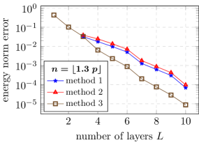
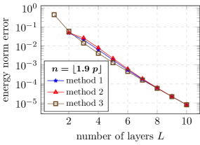
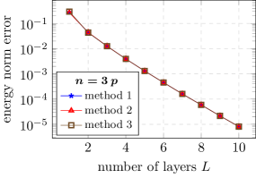
Example 7.1.
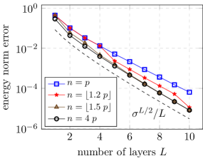
We employ a geometric mesh with grading factor and take piecewise polynomials of degree . In Figure 1, three different error measures are plotted versus the number of refinement layers for different numbers of quadrature points used to calculate the solution :
-
•
Method 1: Use approximation (7.1) with the same number of quadrature points for as for the solution , i.e. .
-
•
Method 2: Use approximation (7.1) and increase the number of quadrature points for the bilinear form to .
-
•
Method 3: Use approximation (7.2) with quadrature points for the reference solution and the bilinear form .
For the cases and all three methods produce nearly identical results, whereas for and the method of calculating the norm has a significant impact. We observe that method 1 overestimates the energy norm error significantly and also increasing the number of quadrature points for the norm calculation (method 2) does not help either. This is consistent with the fact that method 2 does not decrease the consistency error that is made in the Galerkin orthogonality. We also note that for the cases and the computed “energies” were larger than the exact energy so that no errors are reported for these cases in Fig. 1.
The next example is similar to an example in [BFM+23] that shows exponential convergence of -FEM, where the linear system was assembled using the quadrature approach (2.9) in this article.
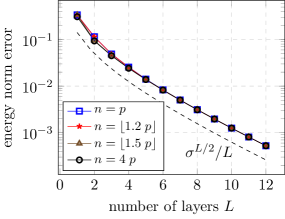
Example 7.2.
We employ a geometric mesh with grading factor and take piecewise polynomials of degree . In Figure 2, the energy norm error (approximation (7.2) with ) is plotted versus the number of refinement layers for different fractional parameters . For the number of quadrature points, we used and, as predicted by Theorem 2.4, we observe exponential convergence with respect to the number of layers noting that . In fact, the convergence behavior is and thus slightly faster than asserted by Theorem 2.4. An argument for this observation is given in [BFM+23, Sec. 4].
Next, we discuss the number of quadrature points used. Although Theorem 2.4 suggests that a choice of quadrature points and in particular for all suffices to obtain exponential convergence, the rate, or more precisely, the constant in the exponent, is impacted by the choice of .
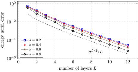
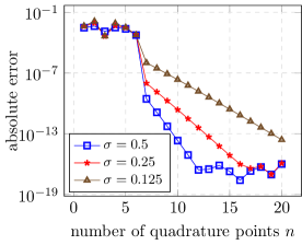
Example 7.3.
Figure 3 plots the energy norm error (approximation (7.2) with ) for different numbers of quadrature points versus the number of layers for two different choices of grading parameters, and . Again, we choose and fix the fractional parameter . We notice that the grading factor has a direct impact on the number of quadrature points needed to achieve the same accuracy. For the smaller , the rate of the exponential convergence depends on the choice of , while, for , the convergence always appears to be . This can also be observed in the theoretical estimates in Theorem 2.4 as the term may be dominant in the case of small .
Finally, we consider the elementwise contributions in Lemma 5.5 and observe exponential convergence for two different configurations.
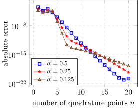
Example 7.4.
Figure 4 considers the case of adjacent elements (left) and separated elements (right) in a geometric mesh with layers and different grading parameters (see Def. 2.2). We plot the absolute quadrature errors for two integrated Legendre polynomials and versus the number of quadrature points . On the reference domain they are defined as
| (7.4) |
where denotes the -th Legendre polynomial. We used with 50 quadrature points, as the reference solution and observe the predicted exponential convergence rate as well as that the rate decreases with . This is in line with Lemma 5.5 since as . We stress that Figure 4 shows the absolute error; the final relative error is close to machine precision.
Acknowledgments
BB and JMM gladly acknowledge financial support by Austrian Science Fund (FWF) throughout the special research program Taming complexity in PDE systems (grant SFB F65, DOI:10.55776/F65).
References
- [AB17] G. Acosta and J.P. Borthagaray. A fractional Laplace equation: regularity of solutions and finite element approximations. SIAM J. Numer. Anal., 55(2):472–495, 2017.
- [ABB17] G. Acosta, F.M. Bersetche, and J.P. Borthagaray. A short FE implementation for a 2d homogeneous Dirichlet problem of a fractional Laplacian. Comput. Math. Appl., 74(4):784–816, 2017.
- [AG18] M. Ainsworth and C. Glusa. Towards an efficient finite element method for the integral fractional Laplacian on polygonal domains. In Contemporary computational mathematics—a celebration of the 80th birthday of Ian Sloan. Vol. 1, 2, pages 17–57. Springer, Cham, 2018.
- [BBN+18] A. Bonito, J.P. Borthagaray, R.H. Nochetto, E. Otárola, and A.J. Salgado. Numerical methods for fractional diffusion. Comput. Vis. Sci., 19(5-6):19–46, 2018.
- [BFM+23] B. Bahr, M. Faustmann, C. Marcati, J.M. Melenk, and C. Schwab. Exponential convergence of hp-FEM for the integral fractional Laplacian in 1D. In Spectral and High Order Methods for Partial Differential Equations ICOSAHOM 2020+ 1: Selected Papers from the ICOSAHOM Conference, Vienna, Austria, July 12-16, 2021, pages 291–306. Springer, 2023.
- [BLN20] J.P. Borthagaray, W. Li, and R.H. Nochetto. Linear and nonlinear fractional elliptic problems. In 75 years of mathematics of computation, volume 754 of Contemp. Math., pages 69–92. Amer. Math. Soc., Providence, RI, 2020.
- [Bra07] D. Braess. Finite elements: Theory, fast solvers, and applications in elasticity theory. Cambridge University Press, Cambridge, third edition, 2007.
- [BV16] C. Bucur and E. Valdinoci. Nonlocal diffusion and applications, volume 20 of Lecture Notes of the Unione Matematica Italiana. Springer, [Cham]; Unione Matematica Italiana, Bologna, 2016.
- [CR13] A. Chernov and A. Reinarz. Numerical quadrature for high-dimensional singular integrals over parallelotopes. Comput. Math. Appl., 66(7):1213–1231, 2013.
- [CS12] A. Chernov and C. Schwab. Exponential convergence of Gauss-Jacobi quadratures for singular integrals over simplices in arbitrary dimension. SIAM J. Numer. Anal., 50(3):1433–1455, 2012.
- [CSW16] S. Chen, J. Shen, and L.-L. Wang. Generalized Jacobi functions and their applications to fractional differential equations. Math. Comp., 85(300):1603–1638, 2016.
- [CvPS11] A. Chernov, T. von Petersdorff, and C. Schwab. Exponential convergence of quadrature for integral operators with Gevrey kernels. ESAIM Math. Model. Numer. Anal., 45(3):387–422, 2011.
- [CvPS15] A. Chernov, T. von Petersdorff, and C. Schwab. Quadrature algorithms for high dimensional singular integrands on simplices. Numer. Algorithms, 70(4):847–874, 2015.
- [DDG+20] M. D’Elia, Q. Du, C. Glusa, M. Gunzburger, X. Tian, and Z. Zhou. Numerical methods for nonlocal and fractional models. Acta Numer., 29:1–124, 2020.
- [DL93] R.A. DeVore and G.G. Lorentz. Constructive approximation, volume 303. Springer Science & Business Media, 1993.
- [FB23] B. Feist and M. Bebendorf. Fractional Laplacian–quadrature rules for singular double integrals in 3D. Comput. Methods Appl. Math., 23(3):623–645, 2023.
- [FMMS23] M. Faustmann, C. Marcati, J.M. Melenk, and C. Schwab. Exponential convergence of -FEM for the integral fractional Laplacian in polygons. SIAM J. Numer. Anal., 61(6):2601–2622, 2023.
- [Heu14] N. Heuer. On the equivalence of fractional-order Sobolev semi-norms. Journal of Mathematical Analysis and Applications, 417(2):505–518, 2014.
- [HMS96] H. Holm, M. Maischak, and E. P. Stephan. The -version of the boundary element method for Helmholtz screen problems. Computing, 57(2):105–134, 1996.
- [JZ23] B. Jin and Z. Zhou. Numerical treatment and analysis of time-fractional evolution equations, volume 214 of Applied Mathematical Sciences. Springer, Cham, 2023.
- [Kar19] G.E. Karniadakis, editor. Handbook of fractional calculus with applications. Vol. 3. De Gruyter, Berlin, 2019. Numerical methods.
- [KM03] B. N. Khoromskij and J. M. Melenk. Boundary concentrated finite element methods. SIAM J. Numer. Anal., 41(1):1–36, 2003.
- [KPP13] M. Karkulik, D. Pavlicek, and D. Praetorius. On 2D newest vertex bisection: optimality of mesh-closure and -stability of -projection. Constr. Approx., 38:213–234, 2013.
- [KS05] G.E. Karniadakis and S.J. Sherwin. Spectral/ element methods for computational fluid dynamics. Numerical Mathematics and Scientific Computation. Oxford University Press, New York, second edition, 2005.
- [LPG+20] A. Lischke, G. Pang, M. Gulian, F. Song, C. Glusa, X. Zheng, Z. Mao, W. Cai, M.M. Meerschaert, M. Ainsworth, and G.E. Karniadakis. What is the fractional Laplacian? A comparative review with new results. J. Comput. Phys., 404:109009, 62, 2020.
- [LZZ19] A. Lischke, M. Zayernouri, and Z. Zhang. Spectral and spectral element methods for fractional advection-diffusion-reaction equations. In Handbook of fractional calculus with applications. Vol. 3, pages 157–183. De Gruyter, Berlin, 2019.
- [Mai95] M. Maischak. Hp-Methoden für Randintegralgleichungen bei 3D-Problemen: Theorie und Implementierung. PhD thesis, Universität Hannover, 1995.
- [McL00] W. McLean. Strongly elliptic systems and boundary integral equations. Cambridge University Press, 2000.
- [MS98] J.M. Melenk and C. Schwab. hp FEM for Reaction-Diffusion Equations I: Robust Exponential Convergence. SIAM journal on numerical analysis, 35(4):1520–1557, 1998.
- [MS18] Z. Mao and J. Shen. Spectral element method with geometric mesh for two-sided fractional differential equations. Adv. Comput. Math., 44(3):745–771, 2018.
- [Sch98] C. Schwab. p-and hp-finite element methods: Theory and applications in solid and fluid mechanics. Oxford: Clarendon Press, 1998.
- [SS11] S.A. Sauter and C. Schwab. Boundary element methods, volume 39 of Springer Series in Computational Mathematics. Springer-Verlag, Berlin, 2011. Translated and expanded from the 2004 German original.
- [SS19] J. Shen and C. Sheng. Spectral methods for fractional differential equations using generalized Jacobi functions. In Handbook of fractional calculus with applications. Vol. 3, pages 127–155. De Gruyter, Berlin, 2019.
- [Ste08] R. Stevenson. The completion of locally refined simplicial partitions created by bisection. Math. Comp., 77(261):227–241, 2008.
- [ZK13] M. Zayernouri and G.E. Karniadakis. Fractional Sturm-Liouville eigen-problems: theory and numerical approximation. J. Comput. Phys., 252:495–517, 2013.
- [ZWSK24] M. Zayernouri, L.-L. Wang, J. Shen, and G.E. Karniadakis. Spectral and Spectral-Element Methods for Fractional Ordinary and Partial Differential Equations. Cambridge University Press, 2024.