Adaptive Event-triggered Control with Sampled Transmitted Output and Controller Dynamics
Abstract
The event-triggered control with intermittent output can reduce the communication burden between the controller and plant side over the network. It has been exploited for adaptive output feedback control of uncertain nonlinear systems in the literature, however the controller must partially reside at the plant side where the computation capacity is required. In this paper, all controller components are moved to the controller side and their dynamics use sampled states rather than continuous one with the benefit of directly estimating next triggering instance of some conditions and avoiding constantly checking event condition at the controller side. However, these bring two major challenges. First, the virtual input designed in the dynamic filtering technique for the stabilization is no longer differentiable. Second, the plant output is sampled to transmit at plant side and sampled again at controller side to construct the controller, and the two asynchronous samplings make the analysis more involving. This paper solves these two issues by introducing a new state observer to simplify the adaptive law, a set of continuous companion variables for stability analysis and a new lemma quantifying the error bound between actual output signal and sampled transmitted output. It is theoretically guaranteed that all internal signals in the closed-loop system are semiglobally bounded and the output is practically stabilized to the origin. Finally, the numerical simulation illustrates the effectiveness of proposed scheme.
Index Terms:
Event-triggered control; Sampled transmitted output; Sampled controller dynamics; Dynamic filtering.I Introduction
Network control, as an integrated technology of computation, communication and physical process, plays an increasingly important role in critical infrastructure, due to its advantages in improving control efficiency and reducing control cost [1]. To achieve more efficient network control, the key lies in how to reduce the communication and computational burdens on the premise of ensuring the closed-loop system’s stability. Event-triggered control has been proved effective in reducing these burdens and used to control satellites [2], unmanned aerial vehicles [3] and robots [4]. Compared with traditional sample-date control, the event-triggered control can effectively reduce signal transmission from controller side to plant side [5].
A lot of progress has been made for the event-triggered control, as pointed out in [2, 3, 4, 5], [6, 7, 8, 9, 10, 11, 12, 13, 14] and references therein, but there are still some limitations. In [7, 8], the event-triggered control algorithms are proposed for a class of systems with and without uncertainties. In [9], adaptive event-triggered control for strict-feedback systems is considered. These schemes are based on real-time monitoring of system state, that means although control signal is not transmitted to plant side during the triggering interval, event detector located at controller side must continuously access state signals at the plant side to determine whether the control signal needs to be updated. This undoubtedly increases the communication in the channel from the plant side to controller side, and also consumes additional network bandwidth. Although output feedback based event-triggered control algorithms are proposed in [10, 11, 12, 13], the real-time monitoring behavior still exists. This problem has been recently addressed in [14] using dynamic filtering technique, where an event detector is constructed at the plant side to determine whether the output signal needs to be transmitted. However, the dynamic filter as the controller component must reside at the plant side such that the dynamic filtering technique can be applicable. Therefore, the computation capacity is also needed at the plant side. Based on [14], intermittent feedback control algorithm is further extended to interconnected systems [15, 16], multi-agent systems [17], while the constant checking behavior of trigger condition at plant side still exists.
This paper proposes an event-triggered adaptive output feedback control algorithm. Compared with [14], we move all components of the controller to the controller side and thus remove the requirement of computation capacity at the plant side. However, it brings a challenge that the virtual input designed in the dynamic filtering technique is no longer differentiable. The main features and contributions of this paper are summarized as follows. (1) Two event detectors are constructed. One is located at the plant side to trigger output transmission, and the other one resides at the controller side to trigger the update of control signal and the controller dynamics. As a result, the transmission between controller side and plant side is intermittent, and the corresponding continuous variables can be calculated by simple algebraic equation rather than numerical integration of the vector function. (2) The controller uses the value of transmitted output from the plant side sampled at the time instance triggered by the event detector at the controller side. A new lemma is introduced to analyze the error bound between actual output signal and sampled transmitted output, which plays an important role in stability analysis. Compared to [14, 15, 16, 17], we only need to check whether there is a new output signal arrival, and calculate the variation of new output signal to determine the next triggering instance, thus the constant checking behavior of event condition at controller side is avoided. (3) A set of companion variables is introduced and backstepping method with dynamic filter is adopted to solve the issue that the virtual input is no longer differentiable caused by sampled output and controller dynamics. Semi-globally practical stability is guaranteed, which is a sacrifice of control accuracy for the introduction of two event detectors when compared to asymptotic stability. (4) A new state estimator and a novel coordinate transformation for the backstepping design procedure such that parameter estimation law is only introduced in the first step, thus simplifying the adaptive law structure compared with [14].
The rest of paper is organized as follows. Section II presents the system model, event-triggered mechanism and control objective. Section III proposes the triggering conditions, elaborates the state observer, adaptive law and dynamic filter, and proves the closed-loop system’s stability. Section IV verifies the effectiveness of proposed control algorithm with a numerical example, and Section V concludes the paper.
II Notations and Problem Formulation
II-A Notations
and denote the set of real numbers and the -dimensional Euclidean space, respectively. denotes the -dimensional square matrix whose elements are all real numbers. denotes the set of nonnegative integers. Unless otherwise specified, denotes the -norm of a vector or matrix. is the set of all first-order differentiable functions.
II-B Problem Formulation
Consider the following nonlinear system in output-feedback form, as studied in [14, 10], and Section 7 of [18],
| (1) | ||||
where , , denote state, output and control input, respectively. is an unknown constant satisfying . are known nonlinear functions with not necessarily being zero and satisfy the Lipschitz condition.
Assumption II.1
The function is function and satisfies the Lipschitz continuity, i.e., there exist known parameters such that
| (2) |
for where is a closed set. And the first partial derivative with respect to satisfies
| (3) |
where .
Remark II.1
In this paper, our proposed algorithm is also applicable for the case that different relative degrees contain different unknown scalar parameters, i.e, , , with for or even they contain different unknown vector parameters, i.e, , , with . For the simplicity of presentation, we only consider the system has one unknown scalar parameter . The proposed algorithm is also effective in output-feedback chain-integrator system, i.e, , , , which is a special case of (1) with for . It’s worth noting that the Lipschitz continuity of is also required for event-triggered control system in [6, 14].
For continuous-time stabilization of the system (1), to tackle the output measurement and the existence of uncertain parameter, the state observer, adaptation dynamics and dynamic filter are usually proposed, respectively, as
| (4) |
Together with (4), the controller can be constructed as
| (5) |
The -dynamics can be designed recursively by the backstepping technique [19, 20].
In this paper, we consider the stabilization control in a networked environment, that is the plant (1) and controller composed of (4) and (5) reside in the two different locations and communicate over the network, as illustrated in Fig 1. The output , controller are transmitted over the network. In order to reduce the communication, information transmission is schedule by the event detectors at the plant (ED1) and controller sides (ED2). Denote the triggering sequence of event detectors at the plant and controller side as and , respectively, where . Then, the information, that is received by the controller and plant sides and both kept by corresponding zero-order holder (ZOH), is denoted respectively as
| (6) | ||||
where is the value of transmitted output sampled at time . Note that and are piecewise continuous.
When we seek the values of in the second equation of (6), it typically requires the integration of the dynamics in (4). For instance, , and where we replace as due to (6). In order to further reduce the computational burden, we use sampled value of to construct the controller dynamics. The controller in the paper is given in the form of
| (7) | ||||
for and . Note that although a more general sampling scheduler can be used, we choose to trigger sampling simultaneously with ED2 for the sake of presentation simplicity. The benefit of (7) over (4) and (5) is that the value can be calculated by simple algebraic equation rather than numerical integration of the vector function. For instance,
| (8) |
where and are constant. The controller (7) can also be implemented by an analog integration circuit rather than on a computing unit. As will be explained later, this mechanism can be exploited to directly estimate next triggering instance of some event conditions and thus simplify the event check.
Remark II.2
In [14], the information transmitted between the plant and controller sides is also event-triggered. Although the state observer and adaptation dynamics reside at the controller side, the dynamic filter resides at the plant side to consume the continuous output signal , where the computation capacity is demanded. In this paper, we move all components of the controller to the controller side, but it brings a challenge that the virtual input designed in the backstepping technique is no longer first-order differentiable. We will tackle this issue in the next section.
The objective is to design the controller and event-triggered laws at the plant and controller sides such that all signals of the closed-loop system are semiglobally bounded and the output is practically stabilized to the origin, i.e., there exists a such that .
III Main Results
In this paper, the triggering law of ED1 is designed as
| (9) |
where is the sampling error of output and is a design parameter.
As will be elaborated in Section III-A, the state of the estimator is decomposed as . Define , , , and . Let , be design parameters for ED2 where is given in (9) for ED1. Then, the triggering law ED2 is designed as
| (10) |
where stands for ‘logic or’. In what follows, we will elaborate the design of the state observer, adaptive law and stabilization controller, and specify parameters in event-triggered laws.
III-A State Observer
Motivated by [10, 18], we estimate the full state through two dynamics. One is for the part of the plant that does not contain and its state is denoted as , and the other one is for its unknown part and its state is denoted as . - and -dynamics are designed as
| (11) | ||||
| (12) |
where , , , and is chosen so that the matrix
| (13) |
is Hurwitz.
Now we explain the benefit of using the sampled value in the -, -, - and -dynamics by examining the last four conditions in (10). Let , , and . We take as the example. Note that is equivalent to , then can be calculated at
where we note that is a known constant. This idea also applies to calculating , and . Let . Then, triggering condition in (10) can be simplified as . Note that the condition only needs to be checked when the new transmitted output arrives. That means we only check condition at some discrete time instances when . If it is not satisfied for , . Therefore, continuously checking the event condition (10) is avoided.
The next lemma gives the error bound between actual output and sampled transmitted output , whose proof is given in appendix.
Unless otherwise specified, the rest of the analysis is based on time interval . We define the estimation error as
| (15) |
The -dynamics in (1) can be written in a compact form as
| (16) |
where , is denoted in (11) and
| (17) |
By (11), (12), (15) and (16), one has
| (18) |
where we used the fact . Define
| (19) |
where is a positive definite matrix satisfying . The derivative of along dynamics (III-A) is
Using (10), (14) and Young’s inequality leads to
| (20) |
with
where is a design parameter and .
Next, we analyze the property of . Define
Then the time derivative of along dynamics (12) is
Note that where is a known parameter and . Then, the bound of becomes
| (21) |
where .
Remark III.1
The work [14] uses for and as the state observer for system (1). The estimation error is defined as -dynamics with and its dynamics is rendered to admit an input-to-state stable Lyapunov function, , , where , , , are unknown parameter relate to , and is a finite positive constant related to triggering threshold. In order to eliminate the term , the virtual controller to be designed needs to introduce another adaptive law to estimate , i.e, in the first step of backstepping procedures. And the virtual controller is designed as where and denote the estimation of and , respectively. On the other hand, we avoid to use the high gain proposed in the state observer in [21, 22].
III-B Adaptive Law and Dynamic Filter
The adaptive law is designed as
| (22) |
for where is the estimate of unknown parameter and is a design parameter. Let , and be th element of , and in (15), respectively. We adopt dynamic filtering technique in [20] and design the dynamic filter as
| (23) |
where is design parameter. is the virtual input designed as
| (24) | ||||
| (25) |
where and is given in adaptive law (22). in (25) is an intermediate variable defined as
| (26) | ||||
| (27) |
where is the virtual error. We now recursively analyze the property of the virtual error.
Step 1: By (15), (27) and (26), we have , . Then, the derivative of is
| (28) |
with . Backstepping method with dynamic filter requires the virtual input be at least first-order differentiable, however in (24) is piecewise continuous. In order to tackle this issue, we define companion variables , for , , respectively, as
| (29) |
By noting , (28) and (29), one has
where
denotes the parameter estimate error. Define
Then is
| (30) |
where . Now, we first examine
| (31) |
Note that
| (32) |
| (33) |
and
| (34) |
where , and with a design parameter . From (III-B), (III-B) and (III-B), one has
| (35) |
Similar to (III-B)-(35), one has
| (36) |
where , and . Moreover, one has
| (37) |
where . Using (31), (35), (36) and (37) obtains
| (38) |
Next, we examine . Due to
where and , one has
| (39) |
Due to
which means that is first-order differentiable and is piecewise continuous. Let and are positive parameters to be designed later and is selected such that . Then
| (40) |
Combining (20), (21), (III-B), (III-B), (III-B) and (III-B), one has
| (41) |
with
| (42) | ||||
Step : let , be companion variables for , , respectively and defined as
| (43) |
Then, the derivative of is
Define
Similar to step 1, substituting (43) into the derivative of gives
| (44) |
where and are positive parameters to be designed later, is selected such that and
Due to
| (45) |
and recursive steps, is piecewise continuous and is first-order differentiable.
Step : Define , then the derivative of is
| (46) |
where we note .
III-C Controller Design and Stability Analysis
Finally, we design the stabilization controller as
| (47) |
for . Substituting (47) into (46) yields
Denote
| (48) |
with , . And denote
| (49) |
where are feedback gains in (24) and (25), are dynamic filter gains in (23), is the parameter of adaptive law in (22), and are adjustable parameters introduced in the recursive steps.
We suppose state observer gains in (13) are determined before the selection of . Let .
Define the Lyapunov function candidate
| (50) |
Then, we have the following results.
Theorem III.1
Consider the uncertain system (1) satisfying Assumption II.1 and the controller composed of stabilization controller (47), adaptive law (22), state observer (11), (12), filter dynamics (23) under triggering laws (9) and (10). Then there exists a such that for any given positive number there always exists a set of parameters such that the set is a positively invariant set and the solution of the closed-loop system is semiglobally bounded. Moreover, the output is practically stabilized to the origin, and the Zeno behavior is excluded. The procedures of the controller design are organized in Algorithm 1.
Proof: Note that within , variables , , , , have upper bounds , , , , , respectively. They are chosen as
where denotes the minimum eigenvalue of . The proof will be divided into three parts. First, we show the bound of within compact set . Note that
where and
Due to
one has
Since are defined in (25), (43), respectively, then we have and . Similarly, step by step, we can conclude the following inequalities
| (51) |
for some depending on . It’s worth noting that when all elements of are chosen sufficiently small, are made sufficiently small. Therefore, by (51)
Next, we will show that is a positively invariant set and all internal signals in the closed-loop system is semiglobal boundedness. By (15), we have
By (51), satisfies
Let , the derivative of along -dynamics in (11) is bounded as , where where we used the fact that when states stay in the compact set . Therefore, the upper bound of is
| (52) |
Now, we analyze the property of within compact set . By (29), the first partial derivatives of are
Due to , , and , by (3), we have
Similarly, we can derive that is also upper bounded, that is
| (53) |
with depending on , , , , , and increasing as each scalar variable of , , , , increases.
Therefore, within compact set , with the help of (III-B), (44), and (54), can be is bounded by
| (55) |
where and with positive constants and . Note that is defined in (42), , , and is determined by . Then, there exists a such that for any given positive number , there always exists a set of parameter such that (See more detailed parameter selection procedure in Remark III.3).
As a result, on the boundary of . Due to (50), is continuous and no jump will occur at . As a result, is a positively invariant set, i.e., if , then for . Due to the boundedness of , , , and , by (27) and (52), it follows that and are bounded and is also bounded by (15). Hence, all signals of the closed-loop systems are semiglobally bounded.
Invoking comparison lemma for (55) yields
which implies that there exists a such that for and and
| (56) |
where we used .
Finally, we show the Zeno behavior is excluded, that is there exist positive constants , such that , for . First, the derivative of is
Then, is denoted as Suppose that is in the th triggering period generated by (9), that is, . Note that for , for and for . Due to , we obtain holds for . Due to and the fact that , we have
| (57) |
The derivatives of , , , are , , , . Therefore, with (57), can be chosen as
Thus, there is no Zeno behavior. The proof is thus complete.
Remark III.2
Remark III.3
We will show we can find a and select controller parameters to make sure that for any . Let be some constant such that and . Let , , and . Let and . As a result, for any , one can find a sufficiently small such that . First, we note that can be written as with being a function increasing as each element of increases. We choose sufficiently small value for each element of such that . We first assume and postpone to show how parameter selection can guarantee it later. As a result, holds and . Second, we select leading to . Note that and thus . Due to , it leads to . Third, we select such that and then . And we select and then for . Last, we show how to select and to guarantee . We select sufficiently large to make . And we select and then , and a sufficiently large such that for . As a result, .
IV Simulation
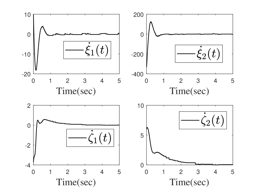
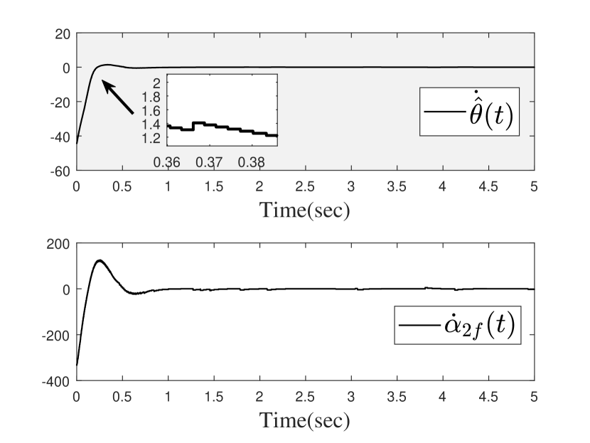
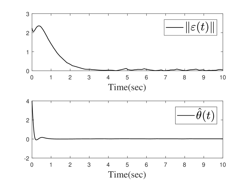
In this section, we give a simulation example to illustrate the proposed control strategy. The system is given as where is an unknown parameter satisfies with . Let . The Lipschitz constant and . Define trigger parameters as . We select , then . are selected as , according to Remark III.3. is chosen as and thus we choose . System initial values as , , , , , satisfying . The simulation time interval is . Fig. 4 is the trajectories of and , where boundedness is shown. Fig. 4 illustrates the control input and Fig. 4 shows that triggering events of ED1 and ED2 are independent of each other. Fig. 7- Fig. 7 show the trajectories of , , and . Fig. 7 shows the boundedness of , which together with Fig. 4, implies the boundedness of and .
| ED1 | ED2 | |
|---|---|---|
| Case 1 | 337 | 148 |
| Case 2 | 212 | 37 |
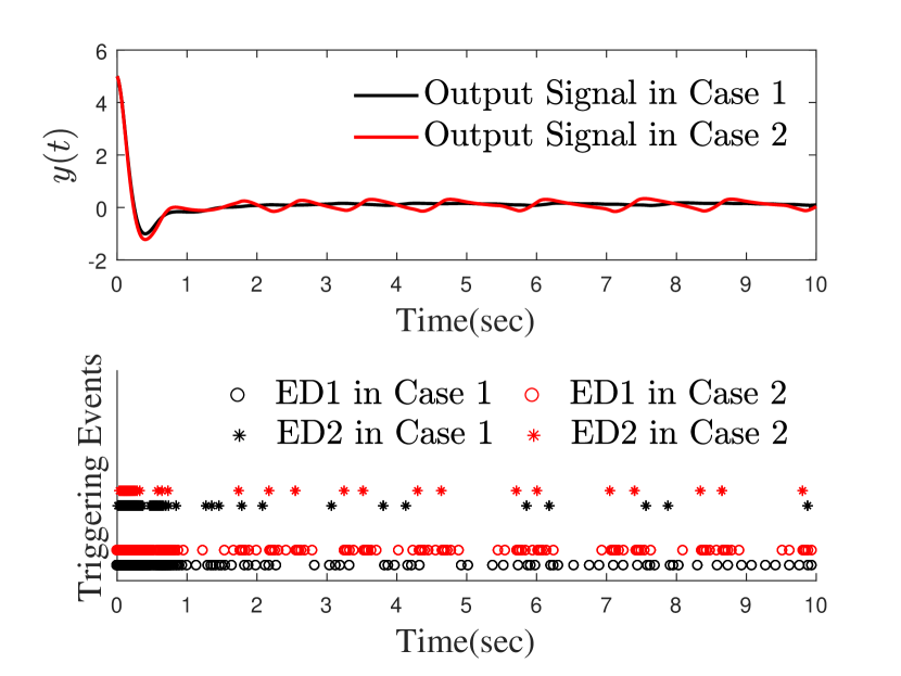
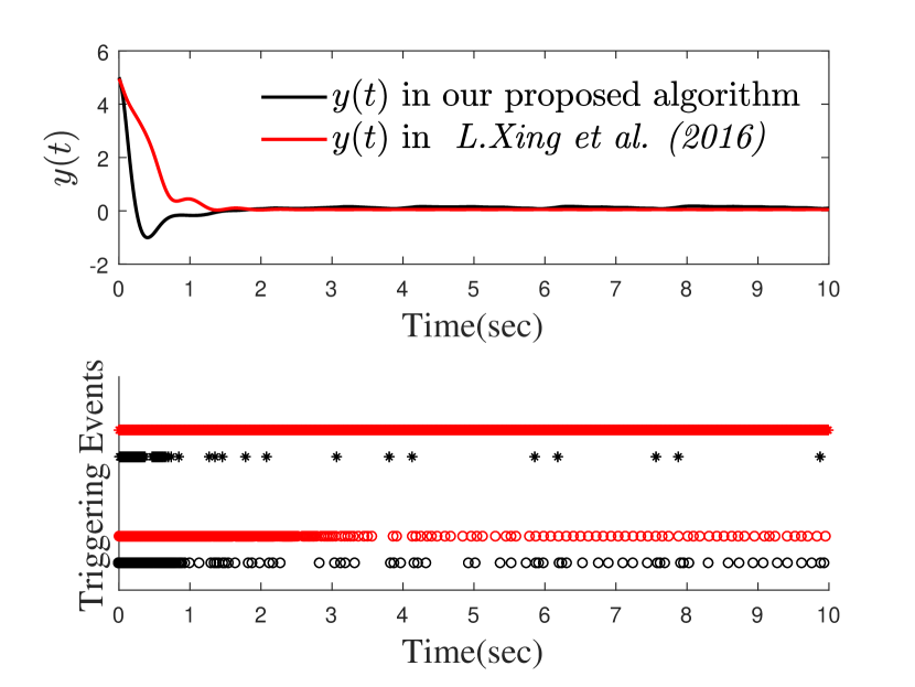
Now, we examine control performance under two set of triggering thresholds. Case 1 is and Case 2 is . The results are illustrated in Fig. 8 and Table. I. It shows different triggering threshold can adjust the ultimate bound of the output and the number of triggering events, and there is a trade-off between transmission frequency and control performance. The small threshold in Case 1 increases the number of the information exchange via the network, and decreases the ultimate bound of the output.
| Our Algorithm | Algorithm in [9] | |
|---|---|---|
| Controller Plant | 337 | 317 |
| Plant Controller | 148 | 1000 |
Furthermore, we compare the proposed scheme with that in [9] where the full states are assumed to be accessible. The event-triggered controller in [9] is designed as
with , , where , , and . The results are shown in Fig. 9 and Table. II. It is observed that when the ultimate bound of the output is essentially the same, our proposed control algorithm requires fewer signal transmissions.
V Conclusion
In this paper, we propose a novel event-triggered algorithm for uncertain nonlinear systems, in which output signal, controller signal and controller dynamics are sampled to be transmitted or be updated by the two event detectors respectively at plant and controller sides. The adaptive law structure is simplified, the requirement of computation capacity at plant side is removed, and the calculation of corresponding continuous variables can be easily implemented by the simple algebraic equation. Furthermore, we solved the issue that the virtual input is no longer differentiable and proved the error bound between actual output signal and sampled transmitted output. It would be very interesting to consider the case that output at plant side is periodically sampled such that the next triggering moment at controller side can be calculated precisely.
References
- [1] F.-L. Lian, J. R. Moyne, and D. M. Tilbury, “Performance evaluation of control networks: Ethernet, controlnet, and devicenet,” IEEE control systems magazine, vol. 21, no. 1, pp. 66–83, 2001.
- [2] W. Liu, Y. Geng, B. Wu, and D. Wang, “Neural-network-based adaptive event-triggered control for spacecraft attitude tracking,” IEEE Transactions on Neural networks and Learning systems, vol. 31, no. 10, pp. 4015–4024, 2019.
- [3] W. Song, J. Wang, S. Zhao, and J. Shan, “Event-triggered cooperative unscented kalman filtering and its application in multi-uav systems,” Automatica, vol. 105, pp. 264–273, 2019.
- [4] J. Yang, F. Xiao, and T. Chen, “Event-triggered formation tracking control of nonholonomic mobile robots without velocity measurements,” Automatica, vol. 112, p. 108671, 2020.
- [5] K. J. Åström and B. Bernhardsson, “Comparison of periodic and event based sampling for first-order stochastic systems,” IFAC Proceedings Volumes, vol. 32, no. 2, pp. 5006–5011, 1999.
- [6] J. Huang, W. Wang, C. Wen, and G. Li, “Adaptive event-triggered control of nonlinear systems with controller and parameter estimator triggering,” IEEE Transactions on Automatic Control, vol. 65, no. 1, pp. 318–324, 2019.
- [7] P. Tabuada, “Event-triggered real-time scheduling of stabilizing control tasks,” IEEE Transactions on Automatic Control, vol. 52, no. 9, pp. 1680–1685, 2007.
- [8] G. D. Khan, Z. Chen, and L. Zhu, “A new approach for event-triggered stabilization and output regulation of nonlinear systems,” IEEE Transactions on Automatic Control, vol. 65, no. 8, pp. 3592–3599, 2019.
- [9] L. Xing, C. Wen, Z. Liu, H. Su, and J. Cai, “Event-triggered adaptive control for a class of uncertain nonlinear systems,” IEEE Transactions on Automatic Control, vol. 62, no. 4, pp. 2071–2076, 2016.
- [10] L. Xing, C. Wen, Z. Liu, H. Su, and J. Cai, “Event-triggered output feedback control for a class of uncertain nonlinear systems,” IEEE Transactions on Automatic Control, vol. 64, no. 1, pp. 290–297, 2018.
- [11] L. Zhu, Z. Chen, D. J. Hill, and S. Du, “Event-triggered controllers based on the supremum norm of sampling-induced error,” Automatica, vol. 128, p. 109532, 2021.
- [12] F. Li and Y. Liu, “Adaptive event-triggered output-feedback controller for uncertain nonlinear systems,” Automatica, vol. 117, p. 109006, 2020.
- [13] L. Zhu and Z. Chen, “A sampling control framework and applications to robust and adaptive control,” arXiv preprint arXiv:2204.13855, 2022.
- [14] Z. Zhang, C. Wen, L. Xing, and Y. Song, “Adaptive event-triggered control of uncertain nonlinear systems using intermittent output only,” IEEE Transactions on Automatic Control, vol. 67, no. 8, pp. 4218–4225, 2022.
- [15] Z. Zhang, C. Wen, K. Zhao, and Y. Song, “Decentralized adaptive control of uncertain interconnected systems with triggering state signals,” Automatica, vol. 141, p. 110283, 2022.
- [16] L. Sun, X. Huang, and Y. Song, “Decentralized intermittent feedback adaptive control of non-triangular nonlinear time-varying systems,” IEEE Transactions on Automatic Control, 2023.
- [17] L. Sun, X. Huang, and Y. Song, “Distributed event-triggered control of networked strict-feedback systems via intermittent state feedback,” IEEE Transactions on Automatic Control, 2022.
- [18] M. Krstic, P. V. Kokotovic, and I. Kanellakopoulos, Nonlinear and adaptive control design. John Wiley & Sons, Inc., 1995.
- [19] M. Krstić, I. Kanellakopoulos, and P. Kokotović, “Adaptive nonlinear control without overparametrization,” Systems & Control Letters, vol. 19, no. 3, pp. 177–185, 1992.
- [20] D. Swaroop, J. K. Hedrick, P. P. Yip, and J. C. Gerdes, “Dynamic surface control for a class of nonlinear systems,” IEEE Transactions on Automatic Control, vol. 45, no. 10, pp. 1893–1899, 2000.
- [21] C. Qian and W. Lin, “Output feedback control of a class of nonlinear systems: a nonseparation principle paradigm,” IEEE Transactions on Automatic Control, vol. 47, no. 10, pp. 1710–1715, 2002.
- [22] J. H. Ahrens and H. K. Khalil, “High-gain observers in the presence of measurement noise: A switched-gain approach,” Automatica, vol. 45, no. 4, pp. 936–943, 2009.
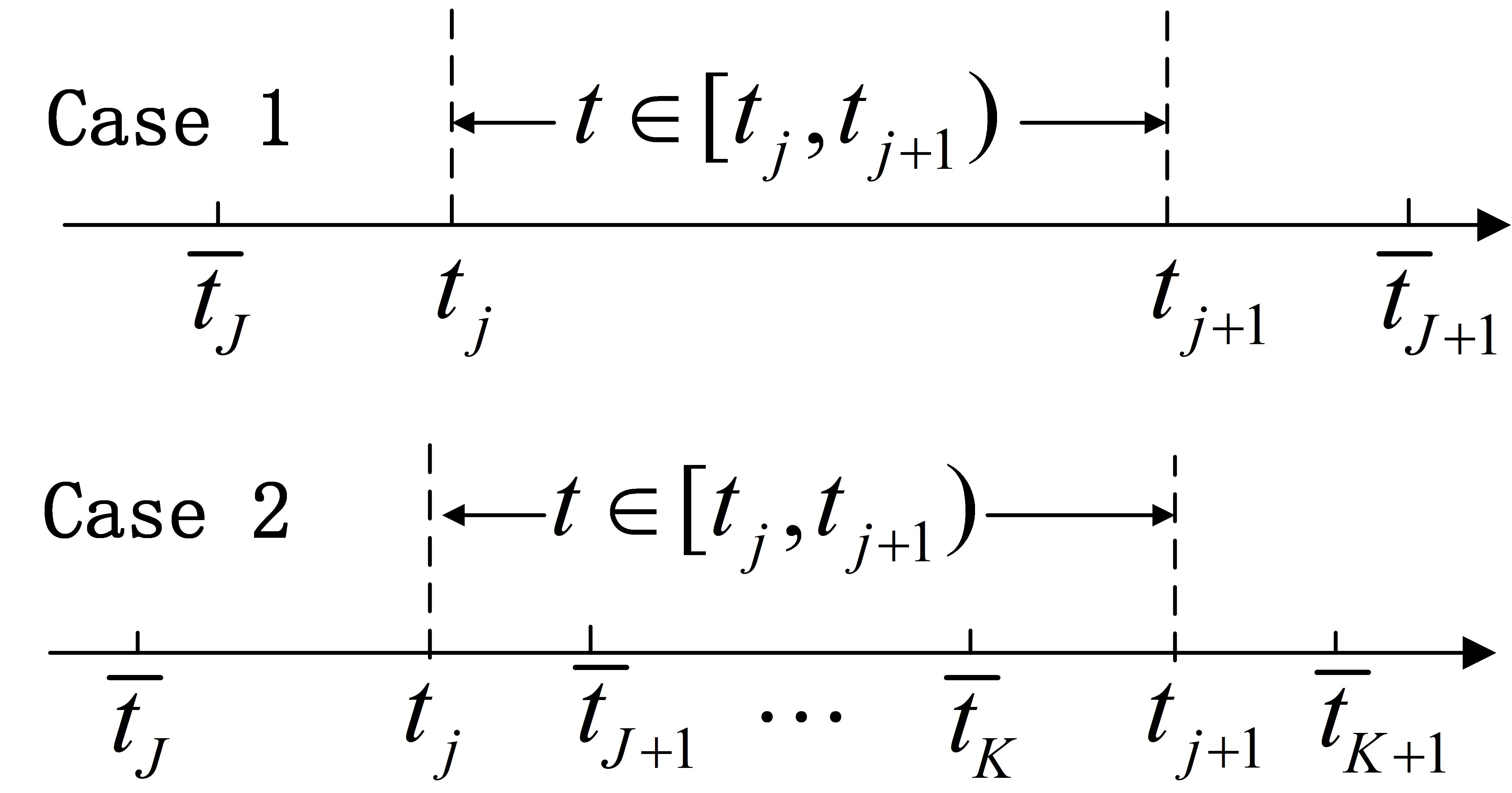
Proof of Lemma III.1: Denote the time interval , where is the triggering instance generated by (9). There are two cases that how the interval is located in . As shown in Fig. 10, Case 1 is for some , and Case 2 is that and for some , , , being triggering instances generated by (9), where .
In Case 1, since holds for and , . By (9), one has
| (59) |
for . In Case 2, when , and , one has
| (60) |
and
When , by (10), holds for . Next, we consider the bound in three intervals, namely , and . First, from Fig. 10, due to , one has
| (61) |
Second, suppose that (9) is triggered times in , that is, where is triggering instances of (9). By (9), for and (), there always exist a continuous function , satisfying , for such that . Therefore holds for . Since and , then
| (62) |
holds for , and thus also holds for . Third, for
| (63) |
By (59), (60), (61), (62) and (Adaptive Event-triggered Control with Sampled Transmitted Output and Controller Dynamics), we prove (14).