Restricted Boltzmann Machine for Modeling Complex Physical Systems: A Case Study in Artificial Spin Ice

Abstract

Restricted Boltzmann machines are powerful tools in the field of generative, probabilistic learning, capable of capturing complex dependencies in data. By understanding their architecture and operational principles, one can employ them for diverse purposes such as dimensionality reduction, feature learning and even representing and analyzing various physical systems. This work aims to provide insights into the capabilities and limitations of restricted Boltzmann machines in modelling complex physical systems in the context of artificial spin ice. Geometrical frustration in artificial spin ice systems creates degeneracies leading to complex states and collective dynamics. From reconfigurable magnonics to neuromorphic computing, artificial spin systems are emerging as versatile functional platforms that go beyond simply imitating naturally occurring materials. Using out of equilibrium data from Monte Carlo simulations of artificial spin ice geometries, this work demonstrates the sensitivity of learning artificial spin ice state distributions with restricted Boltzmann machines. Results indicate that careful application of the restricted Boltzmann machine algorithm can reduce the training data required for feature extraction, which can be used for faster sample generation. Additionally, we demonstrate how the restricted Boltzmann machine can distinguish different artificial spin ice geometries by identifying their respective state distribution features.

I Introduction

Restricted Boltzmann machine (RBM) is a generative, unsupervised, probabilistic deep-learning algorithm[1]. RBM learns a probability distribution over a set of input data and produces new data based on the learnt distribution. It is a system designed to discern and replicate patterns from a dataset, even when those patterns are not immediately apparent to human eyes. This stochastic learning algorithm is used for dimensionality reduction[2], feature learning[3], collaborative filtering[4], and topic modeling[5]. It can be a powerful tool for learning complex features within a joint probability distribution of measurable quantities of the system. A previous example was given by Yevick and Melko[6] who studied the accuracy and behaviour of restricted Boltzmann machines for the 2D Ising model. Here, we use RBM as a tool to investigate the configuration space of a more complex system called artificial spin ice[7] and explore the sensitivity of RBM to the different training parameters and data types.

Artificial spin ice (ASI) systems can display an intricate and complex configuration space which arises from the interplay of the geometrical arrangement of the magnetic elements and the strength and nature of interactions between the elements. Emergent phenomena have been identified from the collective behaviours of magnetic elements. Examples include the formation of magnetic monopoles[8][9], magnetic charge ordering, vertex-based frustration[10][11] and chiral dynamics[12]. The controllable nature of artificial spin ices holds promise for potential applications for data storage, microwave filtering, and energy-efficient machine learning. One key aspect of ASI is that they exhibit complex relaxation dynamics and non-equilibrium behaviours with multiple metastable states. ASI systems have also been proposed as potential platforms for neuromorphic computing[7][13] due to an abundance of accessible nonvolatile states and other useful properties.

Our training data is generated from Metropolis Monte Carlo sampling of two different types of artificial spin ice geometries: square ASI[14] and pinwheel ASI[12][15]. These geometries are illustrated in Fig. 1. These two ASI geometries differ in how they order at low temperatures. While square ASI exhibits antiferromagnetic ordering below its ordering temperature, pinwheel ASI exhibits ferromagnetic ordering.

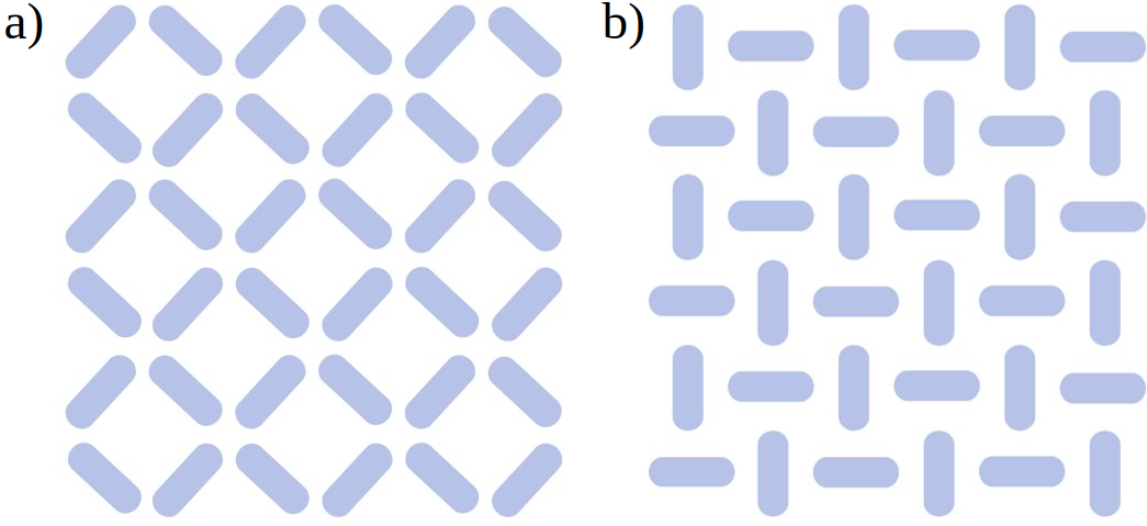
Figure 1: Two artificial spin ice geometries: a) a square and b) a pinwheel. Low-temperature orderings in square ASI and pinwheel ASI are antiferromagnetic and ferromagnetic respectively.

The first part of this paper is dedicated to establishing the necessary models and methods required for collecting the training data and training the RBM. Next, in section III, we demonstrate how well the RBM learns the ASI state distributions regardless of the geometry and its sensitivity to different learning parameters including the temperature at which the training data is generated. We also show that ASI geometries above their ordering temperatures can be classified using trained RBMs in section IV. We conclude in section V by summarizing the results and stressing the significance and potential of our findings.

II Model and Methods

For simplicity, the ASI elements are assumed to be single domains and behave like Ising ‘macro spins’. The magnetic field produced by each element is approximated by a point magnetic dipole located at its centre. This model of interactions treats the elements as individual dipole moments and is a reasonable approximation for well-separated islands. The Hamiltonian is expressed as:

$$\mathcal{H}_{dip}=D\sum_{i\neq j}S_{i}S_{j}\Bigg{[}{\frac{{\hat{\sigma_{i}}\cdot{\hat{\sigma_{j}}}}}{r_{ij}^{3}}}-{\frac{3}{r_{ij}^{5}}}({\hat{\sigma_{i}}}\cdot{{\vec{r}}_{ij}})({\hat{\sigma_{j}}}\cdot{{\vec{r}}_{ij}})\Bigg{]}$$ (1)

where $D=\frac{\mu_{0}\mu^{2}}{4\pi a^{3}}$ provides a characteristic energy scale. $\mu_{0}$ and $\mu$ represent the permeability constant of free space and magnetic moment strength, respectively, while $a$ is the lattice parameter taken as the nearest neighbour distance. $\vec{S_{i}}=\mu S_{i}\hat{\sigma}_{i}$ and $\vec{S_{j}}=\mu S_{j}\hat{\sigma}_{j}$ are magnetic moments of the two elements with spin polarity $S_{i}=S_{j}=\pm 1$, $\hat{\sigma}$’s are the unit vectors parallel to the island easy axes and ${{\vec{r}}_{ij}}$ is the position vector from the i^th element to the j^th element.

For the RBM training, we acquire the data through $600,000$ successive realizations of a $6\times 6$ ASI system generated by a standard Markov chain Metropolis Monte Carlo sampling algorithm at a temperature $T$. The results discussed in this paper are obtained using either a portion of this data or the full set. Before collecting the data, we ensure that the system has stabilized without significant energy fluctuations by running an additional $15,000$ Monte Carlo steps on the system.

A simple RBM consists of two layers of units: one visible to the outside world, representing observable data; and one hidden, connecting only to the visible nodes. The two layers are connected but units within the same layer are not. Every connection has an associated weight $w_{ij}$ and each visible and hidden unit has a bias ascribed to it.

The energy function of an RBM has an Ising-like form[16] and is defined as:

$$E(v,h)=-\sum_{i}a_{i}v_{i}-\sum_{j}b_{j}h_{j}-\sum_{i}\sum_{j}v_{i}w_{i,j}h_{j}$$ (2)

where $w_{i,j}$ is the weight of the interaction between visible unit $v_{i}$ and hidden unit $h_{j}$, $a_{i}$ and $b_{j}$ are the biases for $v_{i}$ and $h_{j}$ respectively. The RBM assumes probabilities of the following form:

$$P(v,h)=\frac{1}{Z}exp(-E(v,h))$$ (3)

where $Z$ is the normalization term. Training restricted Boltzmann machines aims to maximize the expected log probability assigned to a given training set by minimizing the energy function. In this paper, we use a combination of Gibbs sampling[17] and contrastive divergence[18] to maximize the expected log probability of the visible vector $v$. Details of the RBM training process are included in Appendix VI.

The RBM consists of 36 visible units to match the number of spins in a $6\times 6$ lattice. We divide the training set into small batches of $50$ to allow matrix-matrix GPU multiplication to be used. We initialize the biases in Eq. 2 to zero and select initial weights from a standard normal distribution. Through trial and error, we determine the two critical hyper-parameters, the number of hidden nodes and the learning rate[19]. Following Hinton’s guidelines and additional experimentation, our tests indicate that 36 hidden nodes provide optimal learning performance based on training errors. Training errors are computed from the sum of squared errors (obtained from the element-wise difference between the input vector and RBM reconstruction vector) averaged over the batches. The learning rate determines the size of the steps taken towards minimizing the error during optimization[19]. A learning rate that is too high can cause the model to converge too quickly to a suboptimal solution, while a rate that is too low may result in a lengthy training process that might not converge to the best solution. Through experimentation, analysis, and observation, a learning rate of $0.0001$ was determined as optimal. The training data is arranged randomly using a permuted index vector to reduce the correlation between subsequent Metropolis realizations. The trained RBM can use the learnt weights and biases along with random input to reconstruct the training state distribution which can be used to replicate macroscopic quantities of interest, such as the energy and magnetization of the ASI system.

III Data distribution learning with RBM

III.1 Square ASI

We now examine the distribution of square artificial spin ice (ASI) states using RBM. To explore the ASI configuration space, we use the joint system energy and in-plane magnetization components’ state distribution. We show here only the in-plane magnetization along the x-axis, as the magnetization along the y-axis has a similar response and does not add any further information.

Along with training parameters, the restricted Boltzmann machine is also sensitive to the size of the training data and the temperature at which the training data is generated. To analyze this sensitivity quantitatively, a Kullback-Leibler (KL) divergence[20] between the training data distribution and RBM reconstruction is calculated. Kullback-Leibler (KL) divergence is an information-theoretic measure of the difference between two probability distributions. It quantifies the amount to which one probability distribution differs from another that is expected. KL divergence is always non-negative. A KL divergence of 0 indicates that the two distributions are identical. The discrete version of KL divergence has the following general expression for discrete probability distributions $P$ and $Q$ defined on the same sample space:

$$\text{KL}(P||Q)=\sum_{x\in X}P(x)ln\frac{P(x)}{Q(x)}$$ (4)

We represent the ASI state distributions using two variables: system energy and x-component of magnetization. While the geometry of the ASI restricts the system to exhibit only discrete magnetization values, system energy has a continuous form. Accordingly, we use the following form of KL divergence:

$$\text{KL}(P||Q)=\sum_{x}\int_{y}P(x,y)ln\frac{P(x,y)}{Q(x,y)}dy$$ (5)

where the summation is over all possible discrete values of the x-component of magnetization and the integration is over the entire domain of the continuous variable y representing energy of the system.

We use Metropolis Monte Carlo to produce the training data at a given temperature $T$, resulting in $600,000$ successive realizations of a $6\times 6$ square ASI system. Next, we use subsets of this data to train multiple RBMs independently. After the training, we evaluate the RBMs’ performance by testing them on random input data and comparing the resulting reconstructions with $600,000$ Monte Carlo (MC) generated samples at the same temperature using KL divergence. We repeat this process for a temperature range that varies from low to high relative to the square ASI ordering temperature. The ordering temperature of square ASI for our geometry is $T_{c}=2.54$ $D/k_{B}$, consistent with values reported in[21]. Fig. 2 shows the relationship between the training data sizes and the KL divergence value at different temperatures.

Figure 2: KL divergence as a function of square ASI training data sizes at various temperatures. The average is taken over five independent trials.

As the figure demonstrates, overall, the KL divergence value between the training data and the RBM reconstructed data decreases significantly with increasing temperature regardless of the size of the training data. At a high temperature $T=4.5$ $D/k_{B}$, after the training data size crosses a threshold value, the KL divergence value shows a declining trend as the training data size increases. This indicates that RBM performs better when trained with large amounts of high-temperature training data.

Fig. 3 shows the performance of RBM at a low temperature $T=2.1$ $D/k_{B}$. The results are obtained with the RBM trained on $600,000$ Monte Carlo simulated square ASI data and tested on $600,000$ random data using the learnt weights and biases. Included are 2D histogram contour plots showing the distribution of data points across two variables (energy and magnetization along the x-axis) with contours that represent equal probability superimposed on a scatter plot displaying individual data points. The histograms show distributions summed over energy (side) and summed over magnetization (top).

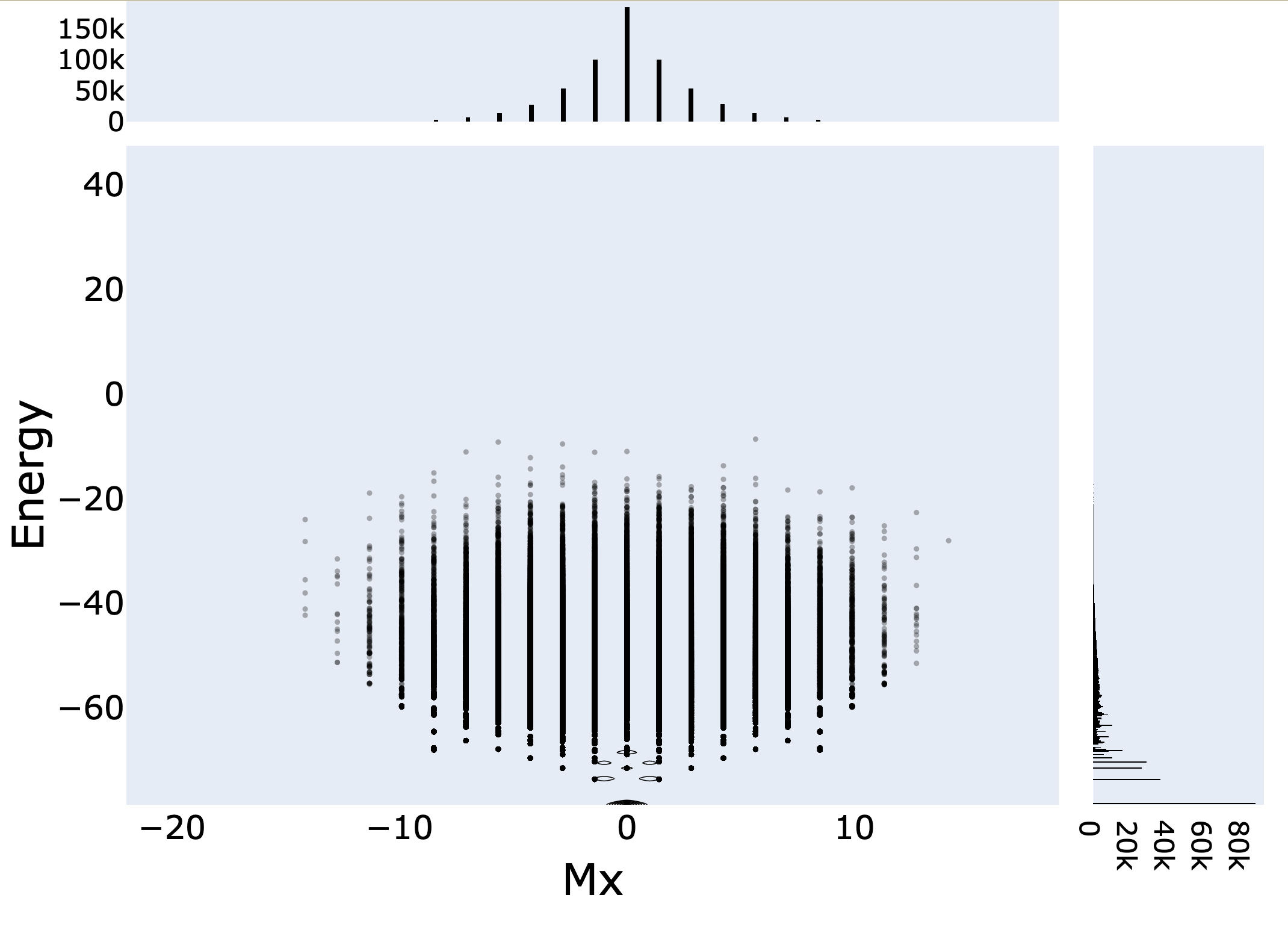
(a)

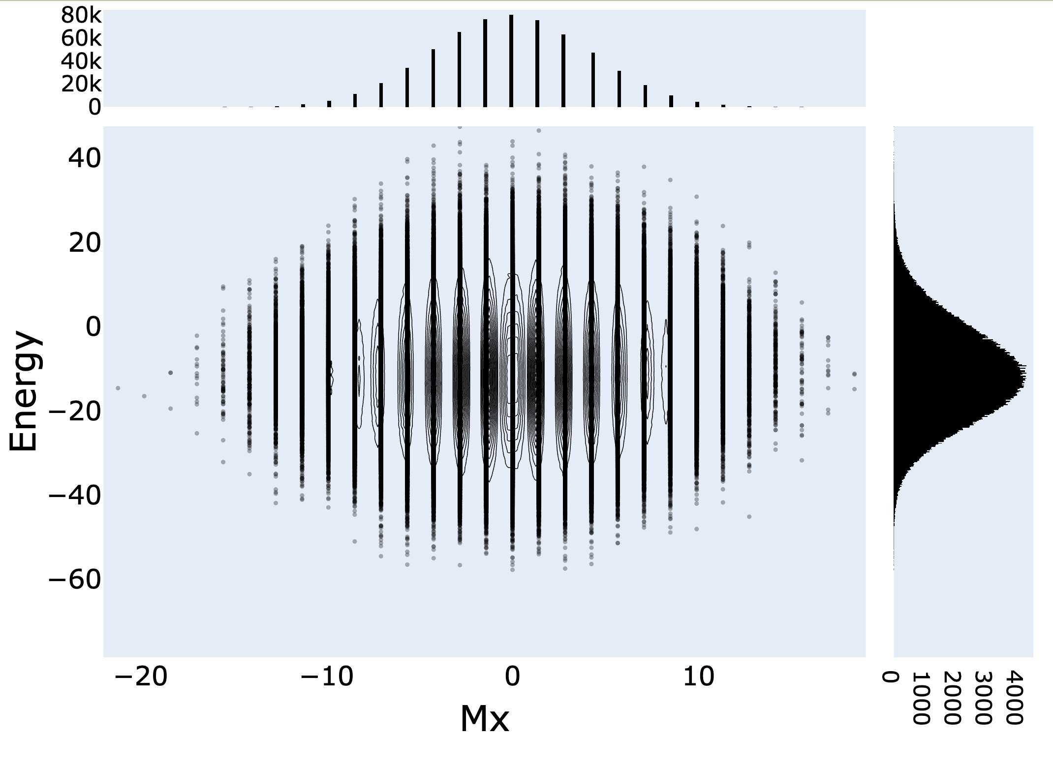
(b)

Figure 3: 2D histogram contour plots showing the distribution of states in energy magnetization space for a) $600,000$ Monte Carlo realizations of a square ASI at $T=2.1$ $D/k_{B}$ and b) $600,000$ Monte Carlo sampled data (at $T=2.1$ $D/k_{B}$) trained RBM reconstruction. The histograms in the insets display the frequencies of energy and magnetization values in their respective data set. This figure shows the trained RBM’s inability to learn the original training data distribution.

Fig. 3 illustrates the RBM’s inability to adequately describe the specifics of the joint energy-magnetization state distribution of the square ASI. In the MC sampled training data (Fig. 3(a)), the energy distribution is skewed and concentrated at very small values. However, in the RBM reconstruction (Fig. 3(b)), the energy distribution appears to be a Gaussian and largely shifted along the +y axis. Similarly, the magnetization distribution in the training data appears to have a sharper peak than the reconstruction. The calculated KL divergence between these two distributions is $1.232$ which signifies a large discrepancy between them.

Now let us investigate how RBM performs when trained with data obtained at a higher temperature. Fig. 4 shows a comparison of results for energy and x component of the magnetization values calculated from $600,000$ Monte Carlo training samples generated at a temperature $T=4.5$ $D/k_{B}$ with the values produced from RBM reconstruction trained on the same dataset. The distributions of the training and reconstructed data are in good agreement between means and higher moments. The most probable states for the Monte Carlo sampled data appear to have zero net magnetization. This is replicated accurately in the reconstructed data set. Although the energy range is shifted along the +y axis in the reconstruction, the energy histogram has a Gaussian form similar to the training data. In this case, the calculated KL divergence value is $0.267$ which is significantly smaller than the previously calculated value of $1.232$ for temperature $T=2.1$ $D/k_{B}$.

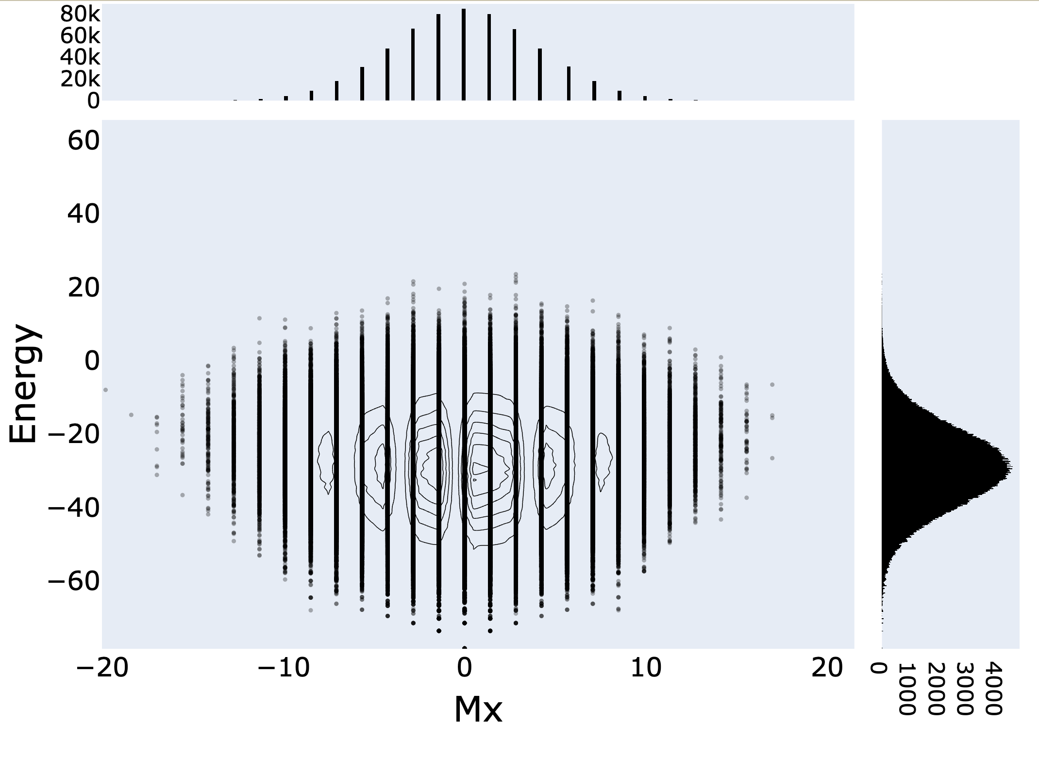
(a)

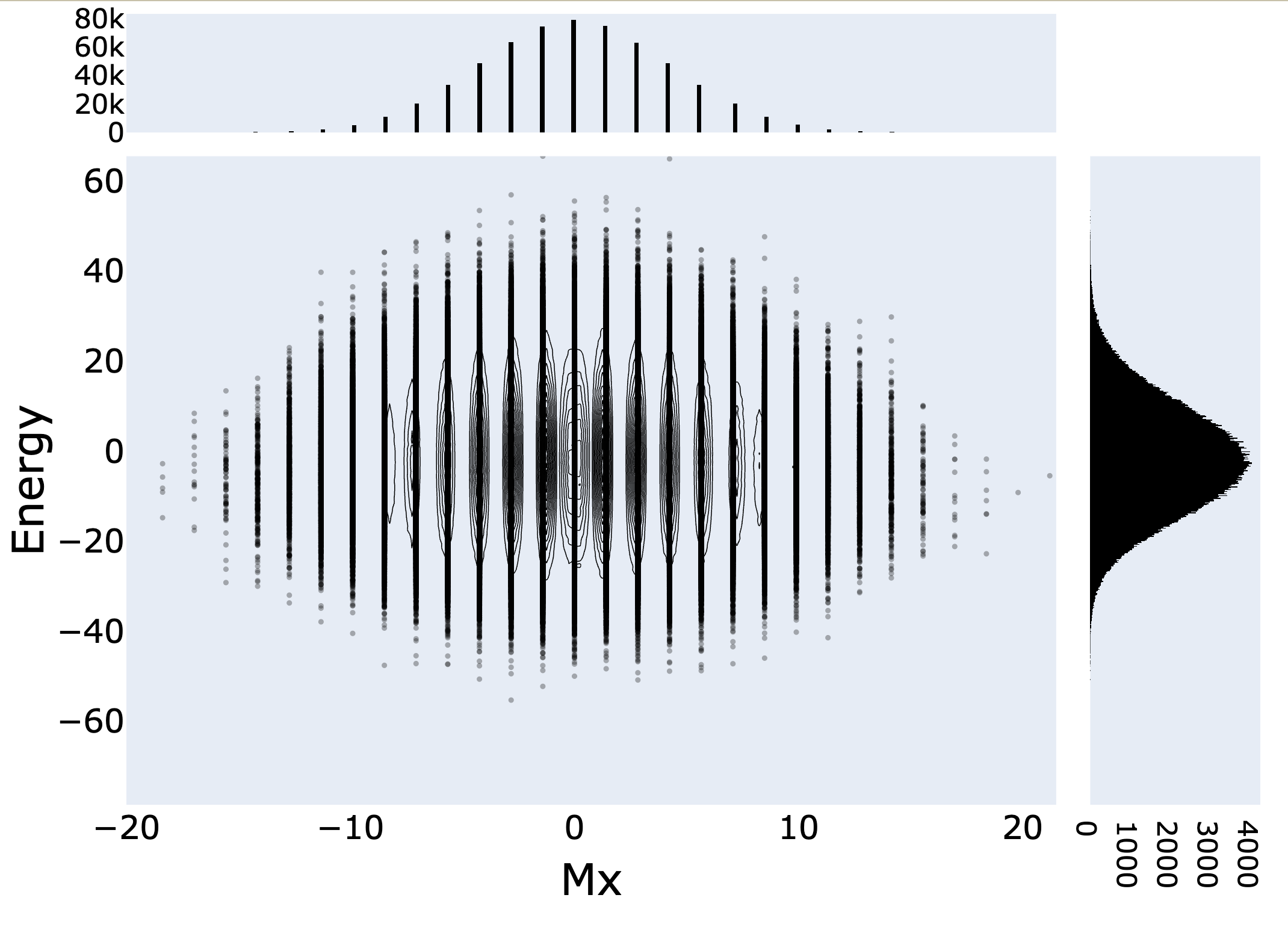
(b)

Figure 4: 2D histogram contour plots showing the distribution of states in energy magnetization space for a) $600,000$ Monte Carlo realizations of a square ASI at $T=4.5$ $D/k_{B}$ and b) $600,000$ Monte Carlo sampled data (at $T=4.5$ $D/k_{B}$) trained RBM reconstruction. The histograms in the insets display the frequencies of energy and magnetization values in their respective data set. The $M_{x}$ values are similar but the energies are shifted.

Interestingly, the RBM trained on the smaller dataset of $360,000$ samples generated at a temperature $T=4.5$ $D/k_{B}$ has a KL divergence of $0.275$ with respect to $600,000$ MC sampled training data set at the same temperature. This suggests that the RBM trained on a small fraction of a dataset can do nearly as well as an RBM trained on the full set.

III.2 Pinwheel ASI

Pinwheel artificial spin ice displays a ferromagnetic ordering at low temperatures. Its ferromagnetic nature at low temperatures enables the formation of domains and domain walls[15]. Studies indicate that for pinwheel ASI, the ordering temperature $T_{c}\approx 0.7$ $D/k_{B}$[22]. As before, to study RBM’s sensitivity to pinwheel ASI training data size and the temperature at which the data is generated, we create $600,000$ Monte Carlo sampled training data from successive realizations of a $6\times 6$ pinwheel ASI system at a range of temperatures. All the RBM parameters are kept the same as for the square ASI. Following the independent training of several RBMs using portions of this data, we compute the KL divergence values between the resulting reconstruction from random input data and $600,000$ Monte Carlo training samples at respective temperatures. The results are displayed in Fig. 5.

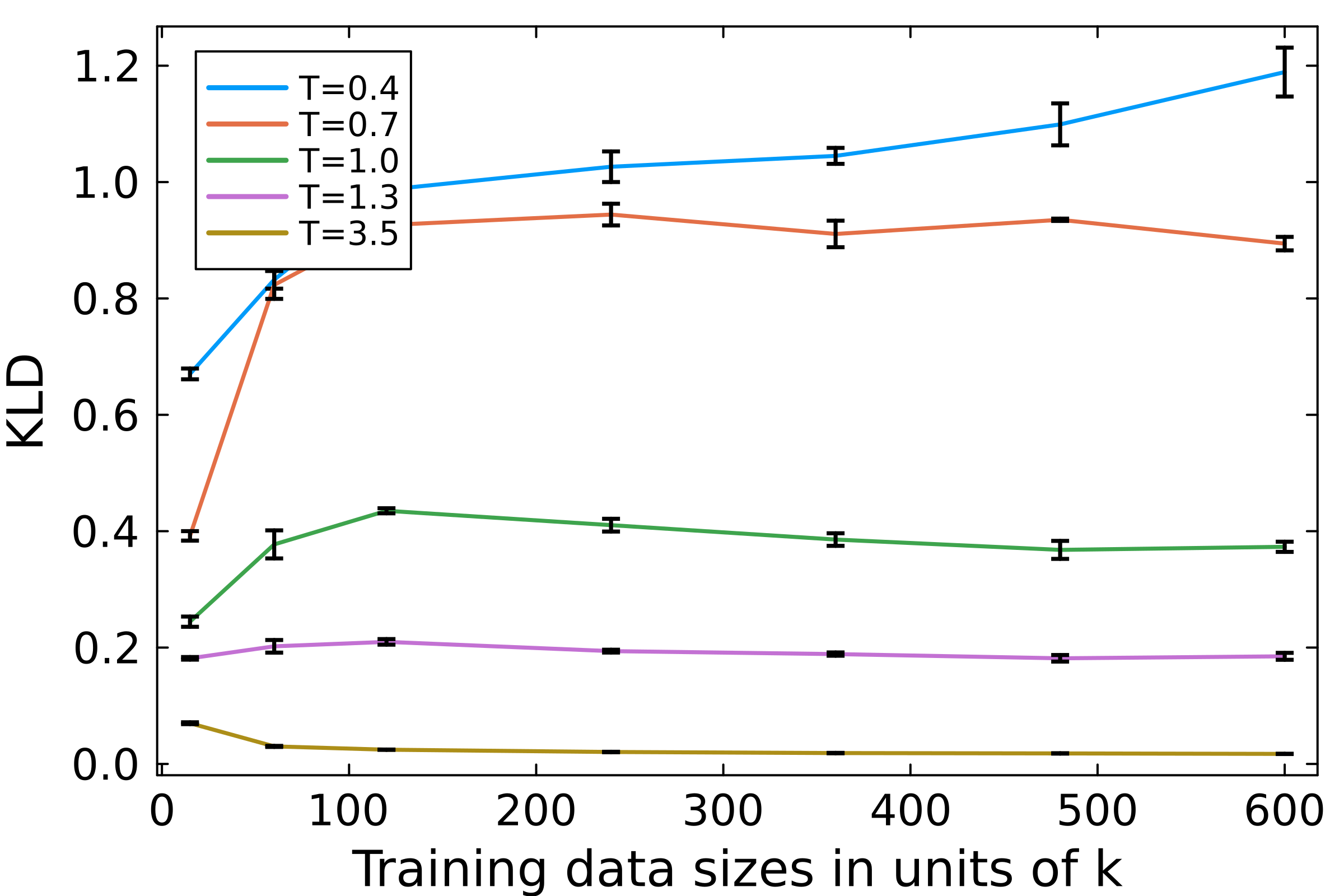
Figure 5: KL divergence as a function of pinwheel ASI training data sizes at various temperatures. The average is taken over five independent trials.

As in the case of square ASI, we can see that RBM performs better at higher temperatures and with large amounts of training data given the smaller KL divergence values. When compared with $600,000$ MC simulated data at $T=0.4$ $D/k_{B}$ with the same data trained RBM reconstruction, KL divergence yields a value of $1.182$ which signifies the RBM’s inability to capture the finer details and characteristics of the training distribution.

Fig. 6 shows a comparison of results for energy and magnetization along the x-axis values calculated from $600,000$ Monte Carlo samples generated at a high temperature $T=3.5$ $D/k_{B}$ along with the 2D histogram contour plot produced from RBM reconstruction trained on $120,000$ Monte Carlo samples. Energy and magnetization histogram plots have Gaussian forms with similar means and higher moments. The two distributions are similar with a KL divergence of $0.022$ between them. When compared instead with the reconstruction from a $600,000$ MC sample trained RBM, KL divergence is calculated to be $0.019$ which is pretty close to the previously calculated value of $0.022$. This again demonstrates that RBM can capture the details of the original distribution with relatively small training data sets.

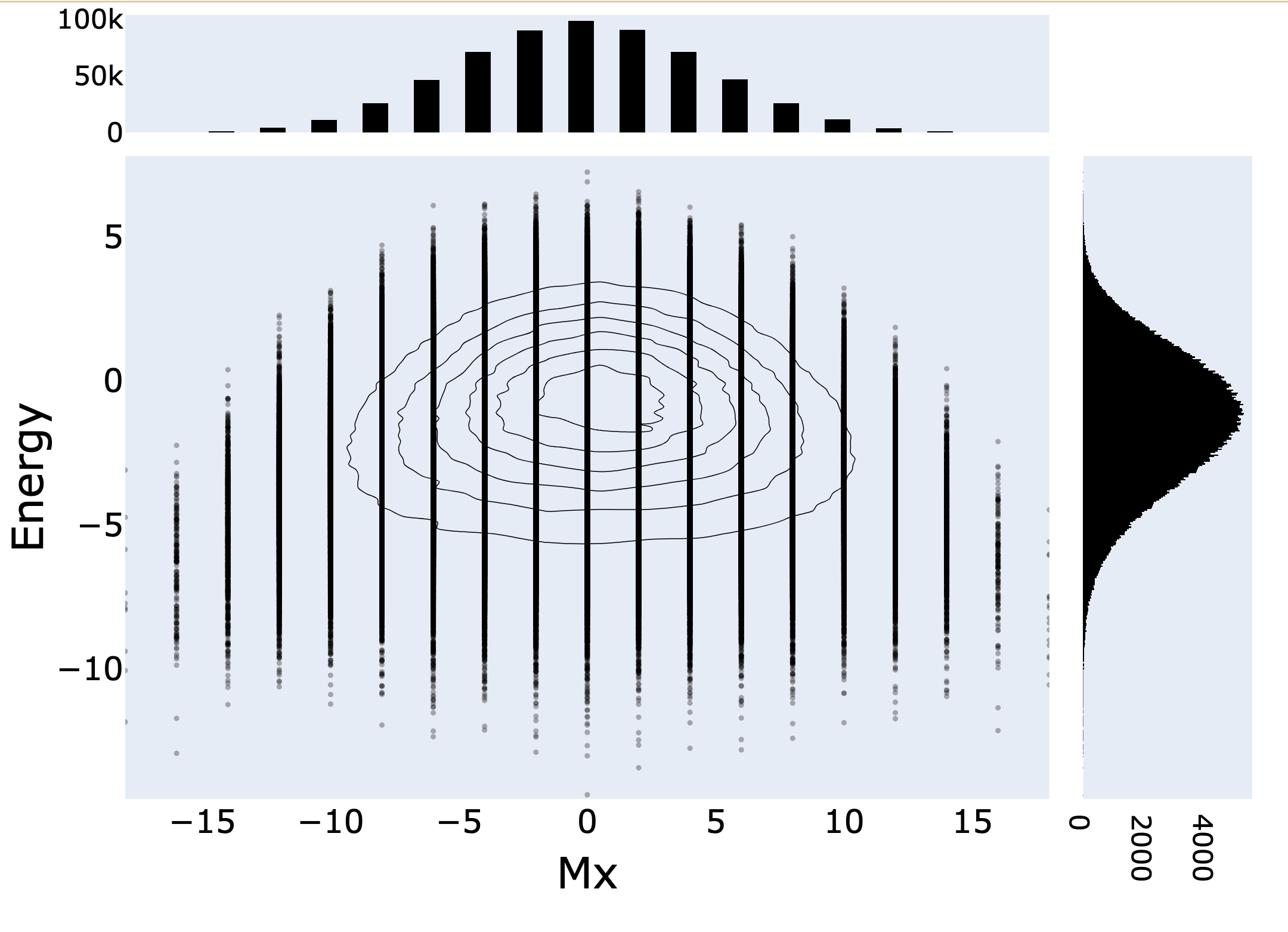
(a)

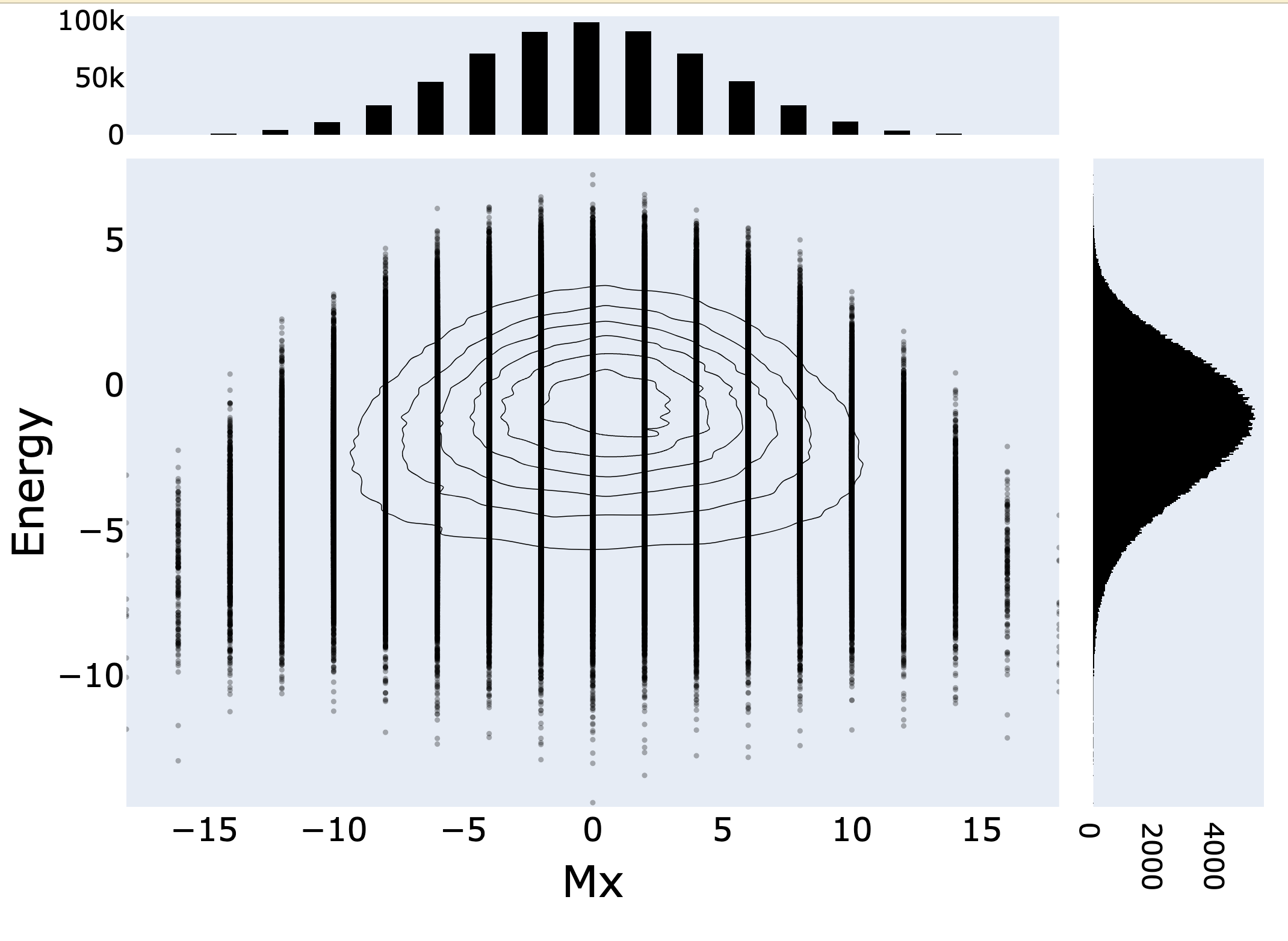
(b)

Figure 6: 2D histogram contour plots showing the distribution of states in energy magnetization space for a) $600,000$ Monte Carlo realizations of a pinwheel ASI at $T=3.5$ $D/k_{B}$ and b) $120,000$ Monte Carlo sampled data (at $T=3.5$ $D/k_{B}$) trained RBM reconstruction. The summed energy and magnetization histograms display the frequencies of energy and magnetization values. Even though the RBM was trained on relatively fewer samples, its reconstruction captures the essence of pinwheel ASI data distribution, including the spread of data points and most probable states. A slight shift in the energy range can be observed.

It is interesting to note the differences between pinwheel and square ASI distributions. Pinwheel ASI has a smaller number of contours, and the contour lines are more symmetric and continuous in nature. This is because of the different ground state orderings in these systems. While square ASI has an antiferromagnetic ground state with a net magnetization of zero, pinwheel ASI has a ferromagnetic ground state with a non-zero net magnetization. At finite temperatures, domains and domain walls are formed in pinwheel ASI which are responsible for the intermediate magnetization values spread across the maximum and minimum $M_{x}$ values having similar energy values.

The reason for RBM’s poor performance at low temperatures could be because the sampled configuration space is smaller at temperatures lower than the ordering temperature since fewer states are frequented there than at higher temperatures. Exploring as many states as possible is needed to capture detailed features across configuration space and RBM is sensitive to the frequency at which states appear.

IV Data classification using RBM

In addition to modelling the probability distribution of data and generating new samples from that distribution, RBMs can also be used for classification tasks. They have been predominantly utilized either to initialize the weight of neural network classifiers or as feature extractors for other classification techniques[23][24]. Later, a self-contained discriminative RBM framework for creating competitive classifiers was proposed[25][26].

We now investigate how well RBMs, in conjunction with a classifier can categorize the two different ASI geometries: square and pinwheel. This is accomplished without altering the RBM’s structure. However, instead of training the RBM on a single type of artificial spin ice data, we use both square and pinwheel ASI data simultaneously for training. The training data for this includes states that are distributed over two separate configuration spaces: $30,000$ square ASI data and $30,000$ pinwheel data generated by the Metropolis Monte Carlo sampling algorithm at a temperature $T=3.5$ $D/k_{B}$ for a $6\times 6$ lattice. The square and pinwheel data are randomly ordered. To test the trained RBM, instead of using random data as before, we use four different classes of data sets: 1) perfect square ASI data, 2) perfect pinwheel ASI data, 3) imperfect square ASI data and 4) imperfect pinwheel ASI data where imperfect ASI data are used to test how well the RBM can distinguish square and pinwheel geometry. In the simulation, the magnetic moment (and thus the strength of each ASI element) is set to unity. To construct an imperfect artificial spin ice, some of the spin elements are designed to interact weakly with others by randomly choosing $4$ spins out of the $36$ spins and setting their magnetic moment values to 0.5. The classification task is accomplished by calculating KL divergence values for reconstructed state distributions and the original square and pinwheel ASI state distributions and based on the KL divergence values, identifying the type of RBM reconstruction, i.e., whether it has a distribution similar to a square or pinwheel ASI.

IV.1 Testing RBM on perfect ASI data

For the first trial, the trained RBM is tested on $60,000$ successive Metropolis Monte Carlo realizations of a perfect $6\times 6$ square artificial spin ice. As expected, the RBM reconstruction has a similar distribution to that of the perfect square ASI data. This claim is verified by KL divergence measurement. When comparing the reconstructed data distribution with the original square ASI data distribution, the KL divergence value is $0.032$. However, when comparing the reconstructed data distribution with the original pinwheel ASI data distribution, the KL divergence measurement yields a value of $0.125$. This indicates that the reconstructed data has a state distribution that matches most closely with that of the square ASI.

Similarly, the trained RBM is tested on $60,000$ successive Metropolis Monte Carlo realizations of a perfect $6\times 6$ pinwheel artificial spin ice and the reconstruction has a closer match with the original pinwheel ASI data distribution. For these two distributions, the KL divergence value is $0.008$, which is much smaller than the KL divergence value of $3.852$ calculated for the comparison between the distributions for the square ASI data and RBM reconstructed data. Table 1 summarizes the KL divergence values for different comparisons.

Table 1: KL divergence values for testing RBM on perfect data

RBM trained on perfect:	RBM tested on perfect:	Reconstruction compared with perfect:	KLD
square + pinwheel	square	square	0.032
		pinwheel	0.125
	pinwheel	square	3.852
		pinwheel	0.008

IV.2 Testing RBM on imperfect ASI data

The artificial spin systems used in experiments are not perfect and include irregularities in the arrangement of nanomagnets, variations in the size or shape of individual nanomagnets, structural imperfections and impurities. To mimic structural defects and other imperfections in terms of magnetizations, we randomly select $4$ spin elements out of $36$ to have half the strength of other elements. This also modifies the interactions between different elements and modifies the ASI state distribution.

Metropolis Monte Carlo sampling is used to generate $60,000$ successive realizations each for an imperfect $6\times 6$ square ASI and an imperfect $6\times 6$ pinwheel ASI. The RBM trained on Monte Carlo simulated $30,000$ perfect square ASI data, and $30,000$ perfect pinwheel data is tested on this imperfect data.

When the trained RBM is tested on imperfect square ASI data, the state distribution of the reconstructed data appears similar to the original square ASI data distribution with a small KL divergence value of $0.118$. This indicates that despite the test data having a slightly different configuration space, RBM can successfully capture the underlying features and relate them to the appropriate training distribution.

Similarly, when the trained RBM is tested on $60,000$ imperfect pinwheel ASI samples, the RBM and the classifier successfully identify the test samples to have a pinwheel ASI-like data distribution. The KL divergence value in this case is $0.015$. This is smaller than the KL divergence value of $0.124$ when comparing the reconstructed distribution with the original square ASI data distribution. The KL divergence measurements for imperfect data are summarized in Table 2.

Table 2: KL divergence values for testing RBM on imperfect data

RBM trained on perfect:	RBM tested on imperfect:	Reconstruction compared with perfect:	KLD
square + pinwheel	square	square	0.118
		pinwheel	0.373
	pinwheel	square	0.124
		pinwheel	0.015

The difference between KLD values for the imperfect square ASI tested RBM reconstruction when compared with the perfect square ASI distribution and when compared with the perfect pinwheel ASI distribution is $0.255$, higher than the KLD difference between the perfect square and perfect pinwheel distribution ($0.093$). Similarly, in the pinwheel case, the KLD difference for imperfect pinwheel ASI data testing is $0.109$, which is significantly smaller than the one for perfect pinwheel ASI data testing ($3.844$). However, this smaller difference is still sufficient to differentiate between these two ASI systems.

V Conclusion

RBMs have been shown to successfully learn the high-temperature state distributions from two different artificial spin ice geometries: square and pinwheel. They learn to encode abstract features of the input, which can represent higher-order correlations and dependencies in the data. This allows the trained RBMs to generate new samples that accurately reflect the statistical properties of the system, enabling further analysis and exploration of the ASI behaviour. In practical experiments, it is crucial to sample a large number of states to study the statistical properties of the system accurately, which can be sometimes time-consuming. RBM can be useful in this regard as it has the capability of capturing the essential statistics of the ASI state distribution from a smaller data set.

Another potential application of RBMs explored in this paper lies in correctly identifying hidden features in the ASI distributions and employing them to classify unknown ASI samples. We show that RBMs can distinguish between different ASI geometries in mixed data. Even if the test data is not ideal, RBMs can correctly identify the characteristic features and the reconstruction mimics the perfect data distribution for the same class. This has significant potential in practice because any experimental realization of ASI is bound to contain defects or disorders in the form of irregularities, dislocations, edge boundaries, impurities etc. So the data obtained from the experiments does not represent a perfect ASI system. It will be interesting to see how RBM can be exploited to make it a valuable tool for unknown sample classification in the future. Careful examination and comparison of RBM reconstructions when trained on perfect ASI data and when trained on imperfect (defected) ASI data might make it possible to infer the distribution of defects present in the imperfect system.

However, there must be a limit to RBM’s capability to recognize defective systems. If there is a significant amount of defects present in a system, RBM might fail to classify that system correctly. The extent to which RBM can identify a defective system needs a thorough investigation. It is also worth studying RBM’s inability to learn ASI state distribution at lower temperatures. It might give us an insight into how RBM learns the hidden correlations between the spin elements and associates proper weights to them.

VI Appendix

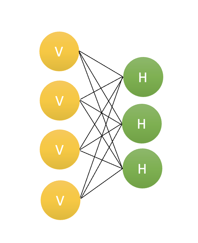
Figure 7: Schematic representation of a restricted Boltzmann machine. Yellow circles are visible units in the first layer. Green circles are probabilistic hidden units in the second layer.

The neurons in the hidden layer receive input data from neurons in the visible layer. The weights are multiplied by the inputs, and the bias is added. The resulting product goes through the activation function. The output of the activation function, which is subsequently applied to the result, determines whether or not the hidden state is activated. Multiple inputs are combined and contribute to the activation of a single hidden node. This process is repeated for all hidden units. Following the activation of the hidden layer neuron, its output value serves as a new input. This new input is multiplied by the same weights as before and combined with the bias of the visible layer. This process is known as either reconstruction or backward pass. The original input and the newly generated input are then compared to assess whether they match. By comparing these inputs, the restricted Boltzmann Machine can evaluate the quality of the reconstruction and adjust its parameters accordingly during the training process. This comparison helps the model learn to recreate the original input as accurately as possible[19].

The RBM model is an energy-based model where the joint probability distribution is defined by its energy function as follows:

$$P(v,h)=\frac{1}{Z}exp(-E(v,h))$$ (6)

In this context, $Z$ represents a partition function that is calculated as the sum of exponential terms across all possible configurations. The probability of a visible vector can be calculated by summing the probabilities of $P(v,h)$ across all possible configurations of the hidden layer[19].

$$P(v)=\frac{1}{Z}\sum_{h}e^{-E(v,h)}$$ (7)

Similarly, the probability of a hidden layer configuration can be calculated by summing the probabilities of $P(v,h)$ over all possible visible vector configurations.

$$P(h)=\frac{1}{Z}\sum_{v}e^{-E(v,h)}$$ (8)

The visible and hidden units are independent. Thus, if there are $m$ visible units and $n$ hidden units, the conditional chance of a visible unit configuration $v$ given a hidden unit configuration $h$ is:

$$P(v|h)=\prod_{i=1}^{m}P(v_{i},h)$$ (9)

And, the conditional probability of $h$ given $v$ is:

$$P(h|v)=\prod_{j=1}^{n}P(h_{j},v)$$ (10)

Using a probabilistic interpretation of the neuron activation function, we have:

$$P(v_{i}=1|h)=\sigma(a_{i}+\sum_{j=1}^{n}w_{ij}h_{j})$$ (11)

$$P(h_{j}=1|v)=\sigma(b_{j}+\sum_{i=1}^{m}w_{ij}v_{i})$$ (12)

where $\sigma$ denotes the logistic sigmoid as an activation function having the following general form:

$$\sigma(x)=\frac{1}{1+e^{-x}}$$ (13)

The sigmoid function is used for binary classification, where the output is a probability between 0 and 1, indicating how likely the input belongs to a particular class. On the other hand, the softmax function is used when there are more than two classes. It outputs a probability distribution over multiple classes.

Training restricted Boltzmann machines aims to maximize the product of the probabilities assigned to a given training set $V$ (a matrix, where each row of it is treated as a visible vector $v$).

$$Max\prod_{v\in V}P(v)$$ (14)

Or, equivalently, maximize the expected log probability of v. The expected log probability is the average of the logarithm of the probabilities assigned to each training example.

$$Max\ \textbf{E}\left[\sum_{v\in V}logP(v)\right]$$ (15)

The contrastive divergence (CD) algorithm is most frequently used to train RBMs by optimizing the weight matrix $W$. The weight update is computed by a gradient descent process incorporating the Gibbs sampling algorithm. Gibbs sampling estimates the posterior distribution of a set of parameters given some observed data. It is utilized to generate samples from a complex probability distribution, where each variable is sequentially updated based on the current values of all other variables. This iterative process continues until the distribution reaches a steady state. Contrastive divergence then comes into play, refining the model’s parameters. It does this by contrasting the updates derived from the data with those obtained from a few iterations of Gibbs Sampling. This comparison helps to align the model’s distribution more closely with the actual data. This is how the contrastive divergence algorithm works:

• Start with a training sample $v$ and calculate the probabilities of the hidden units. Sample a hidden activation vector $h$ from this probability distribution.

• Compute the outer product of $v$ and $h$, which represents the positive gradient.

• From $h$, generate a reconstruction $v^{\prime}$ of the visible units. Then, resample the hidden activations $h^{\prime}$ based on this reconstruction (Gibbs sampling step).

• Calculate the outer product of $v^{\prime}$ and $h^{\prime}$, representing the negative gradient.

• Update the weight matrix $W$ using the positive gradient minus the negative gradient, multiplied by a learning rate.

• Update the biases $a$ and $b$ in a similar manner.