Integrating Amortized Inference with Diffusion Models for Learning Clean Distribution from Corrupted Images

Abstract

Diffusion models (DMs) have emerged as powerful generative models for solving inverse problems, offering a good approximation of prior distributions of real-world image data. Typically, diffusion models rely on large-scale clean signals to accurately learn the score functions of ground truth clean image distributions. However, such a requirement for large amounts of clean data is often impractical in real-world applications, especially in fields where data samples are expensive to obtain. To address this limitation, in this work, we introduce FlowDiff, a novel joint training paradigm that leverages a conditional normalizing flow model to facilitate the training of diffusion models on corrupted data sources. The conditional normalizing flow try to learn to recover clean images through a novel amortized inference mechanism, and can thus effectively facilitate the diffusion model’s training with corrupted data. On the other side, diffusion models provide strong priors which in turn improve the quality of image recovery. The flow model and the diffusion model can therefore promote each other and demonstrate strong empirical performances. Our elaborate experiment shows that FlowDiff can effectively learn clean distributions across a wide range of corrupted data sources, such as noisy and blurry images. It consistently outperforms existing baselines with significant margins under identical conditions. Additionally, we also study the learned diffusion prior, observing its superior performance in downstream computational imaging tasks, including inpainting, denoising, and deblurring.

1 Introduction

Diffusion models (DMs) ho2020denoising ; song2020score ; song2019generative ; sohl2015deep have become a key focus in generative modeling due to their exceptional ability to capture complex data distributions and generate high-fidelity samples. Their versatility has led to successful applications across various data modalities, including images rombach2022high ; dhariwal2021diffusion , videos ho2022imagen ; ho2022video , text li2022diffusion , audio kong2020diffwave , 3D shapes tang2023make ; luo2021diffusion , and scientific domains like molecule design guo2024diffusion ; huang2023mdm . A particularly promising application of DMs is in solving computational imaging inverse problems, which aim to recover the underlying image $\mathbf{x}$ from noisy or corrupted observations $\mathbf{y}$ chung2022diffusion . This can be probabilistically formulated as:

$$p(\mathbf{x}\mid\mathbf{y})\propto p(\mathbf{y}\mid\mathbf{x})p(\mathbf{x}).$$ (1)

where $p(\mathbf{y}\mid\mathbf{x})$ represents the forward model mapping images to observations, and $p(\mathbf{x})$ encodes prior knowledge about the images. Inverse problems are often ill-posed due to noise and corruption, leading to ambiguous solutions. DMs serve as powerful priors because they approximate the gradient of the data’s log-likelihood function $\nabla_{\mathbf{x}}\log p_{data}(\mathbf{x})$, effectively constraining the solution space by leveraging their ability to model complex image distributions, favoring realistic and high-quality reconstructions.

However, training an effective DM typically requires a large dataset of clean images, which can be expensive or sometimes impossible to acquire. For example, in structural biology, 3D protein structures cannot be directly observed, and only low signal-to-noise 2D projections are captured by cryo-electron microscopy (Cryo-EM) nogales2015cryo . Similarly, in astronomy, black hole images are impossible to observe directly. Such scenarios, where only corrupted data is available, are common, especially in scientific applications. This raises the question: is it possible to train DMs on clean data distributions using only corrupted observations?

In this paper, we provide an affirmative answer and introduce a general framework capable of learning clean data distributions from arbitrary or mixed types of corrupted observations. The key insight is to incorporate an additional normalizing flow kingma2018glow that estimates clean images from corrupted observations through amortized inference. The normalizing flow is trained jointly with the DM in a variational inference framework: the normalizing flow generates clean images for training the DM, while the DM in turn imposes an image prior to guide the the normalizing flow model to get reasonable estimations Although this may seem like a chicken-and-egg problem, we demonstrate that a good equilibrium can be reached using an appropriate training strategy. The normalizing flow converges to a good inference function, and the DM converges to the clean data distribution, enabling simultaneous retrieval of clean images and learning of the clean distribution, even when no clean signals are provided. Through extensive experiments, we show that our method significantly outperforms existing approaches across multiple computational imaging applications, including denoising, deblurring, and fluorescent microscopy.

2 Background

2.1 Score-based diffusion models

Score-based diffusion models ho2020denoising ; song2020score ; song2019generative ; sohl2015deep are a class of generative models that leverage stochastic processes to generate high-quality data, such as images or audio. Unlike traditional generative models that directly map latent codes to data samples, these models operate by gradually transforming a simple noise distribution, $\pi\sim\mathcal{N}(\mathbf{0},\mathbf{I})$, into a complex data distribution, $p_{data}$, through a series of small, iterative steps. This process involves a forward diffusion phase, which adds noise to the data, and a reverse diffusion phase, which denoises it. Both phases are governed by stochastic differential equations (SDEs) defined over the time interval $t\in[0,T]$:

$$\begin{split}\text{Forward-time SDE:}\quad d\mathbf{x}&=\mathbf{f}(\mathbf{x},t)dt+g(t)d\mathbf{w},\\ \text{Reverse-time SDE:}\quad d\mathbf{x}&=\left[\mathbf{f}(\mathbf{x},t)-g(t)^{2}\nabla_{\mathbf{x}}\log p_{t}(\mathbf{x})\right]dt+g(t)d\mathbf{\overline{w}},\end{split}$$ (2)

where $\mathbf{w}\in\mathbb{R}^{d}$ and $\mathbf{\overline{w}}\in\mathbb{R}^{d}$ are Brownian motions, $\mathbf{f}(\cdot,t):\mathbb{R}^{d}\rightarrow\mathbb{R}^{d}$ defines the drift coefficient that controls the deterministic evolution of $\mathbf{x}(t)$, and $g(\cdot):\mathbb{R}\rightarrow\mathbb{R}$ is the diffusion coefficient that controls the rate of noise increase in $\mathbf{x}(t)$. At the core of the reverse diffusion process is a neural network, $s_{\theta}$, which is trained to approximate the score function, i.e., the gradient of the log-density $\nabla_{\mathbf{x}}\log p_{t}(\mathbf{x})$. This allows constructing a diffusion process $\mathbf{x}_{t=0:T}$ where $\mathbf{x}_{0}\sim p_{data}$ and $\mathbf{x}_{T}\sim\mathcal{N}(\mathbf{0},\mathbf{I})$. Score-based diffusion models have demonstrated remarkable success in generating high-fidelity data and have become a significant area of research in machine learning and artificial intelligence.

2.2 Diffusion models for inverse problems

Inverse problems aim to recover an underlying signal or image from observations and arise in various fields, such as computational imaging. These problems are often ill-posed due to factors like noise, incomplete data, or non-invertible forward operators ($\mathbf{x}\to\mathbf{y}$) that map the underlying signal $\mathbf{x}$ to observations $\mathbf{y}$. Traditional inverse problem solvers rely on handcrafted priors or regularizers that impose assumptions about the signal’s structure or smoothness. However, these assumptions may lead to suboptimal reconstructions, especially for complex images with intricate details. Diffusion models offer powerful data-driven priors or regularizers for the inversion process Luo2023ACS ; feng2023score . By incorporating the forward operator into the diffusion process using Bayes’ rule, a conditional score function, $\nabla_{\mathbf{x}}\log p_{t}(\mathbf{x}\mid\mathbf{y})$, can be defined, enabling a conditional diffusion process to gradually recover the underlying clean image from noisy observations graikos2022diffusion ; kawar2021snips ; chung2022diffusion . As diffusion models inherently define a sampling approach, they not only provide point estimates but also quantify reconstruction uncertainties, which is valuable for scientific and medical imaging applications song2021solving .

2.3 Learning generative priors from corrupted data

Generative models need large clean datasets to learn accurate data distributions. However, when only corrupted observations are available, directly training generative models on these data may lead to distorted or biased distributions, resulting in poor generative performance and suboptimal priors for inverse problems. A promising approach is learning the clean generative prior directly from corrupted observations. Early approaches like AmbientGAN bora2018ambientgan and AmbientFlow kelkar2023ambientflow have explored this concept for GANs and normalizing flows, respectively. AmbientGAN integrates the forward model into its generator, simulating the measurements of generated images, while its discriminator differentiates between real and simulated measurements. AmbientFlow uses a variational Bayesian framework sun2021deep to train two flow-based models; one predicts clean images from noisy data, and the other models the clean distribution. However, the limited capacity of GANs and flows restricts the modeling of complicated distributions

Recent research has shifted towards training clean diffusion models using corrupted data. Techniques such as AmbientDiffusion daras2023ambient introduce additional corruption during training. As the model cannot distinguish between original and further corruptions, this helps the diffusion model restore the clean distribution. Methods like SURE-Score aali2023solving and GSURE kawar2023gsure utilize Stein’s Unbiased Risk Estimate (SURE) loss to jointly train denoising and diffusion models through denoising score matching. However, these methods often have restrictive assumptions about the type of corruption—SURE-Score is limited to denoising, and AmbientDiffusion to inpainting. This motivates exploring a more generalizable framework for training expressive diffusion models using arbitrary or mixed types of corrupted data.

3 Methods

In this section, we propose a diffusion-based framework to learn clean distribution from corrupted observations, as shown in Fig. 1. Specifically, we first introduce the amortized inference framework with a parameterized normalizing flow for the image inverse problems in Sec. 3.1. Then, we elaborate on how to adopt score-based generative models to approximate image priors in Sec. 3.2. Finally, we discuss the techniques and implementation details for jointly optimizing the normalizing flow and the diffusion prior in Sec. 3.3.

3.1 Amortized inference with normalizing flows

To solve a general noisy inverse problem $\mathbf{y}=f(\mathbf{x})+\eta$, where observations $\mathbf{y}$ are given, $f(\cdot)$ is the known forward model, $\eta\sim\mathcal{N}(\mathbf{0},\sigma_{n}^{2}\mathbf{I})$, we aim to compute the posterior $p(\mathbf{x}\mid\mathbf{y})$ to recover underlying signals $\mathbf{x}$ from corrupted observations $\mathbf{y}$. However, it is intractable to compute the posterior exactly, as the true values of the measurement distribution $p(\mathbf{y})$ remain unknown. Therefore, we consider an amortized inference framework to approximate the underlying posterior with a deep neural network parameterized by $\varphi$. The goal of optimization is to minimize the Kullback-Leibler (KL) divergence between the variational distribution $p_{\varphi}(\mathbf{x}\mid\mathbf{y})$ and the true posterior $p(\mathbf{x}\mid\mathbf{y})$:

$$D_{KL}(p_{\varphi}(\mathbf{x}\mid\mathbf{y})\parallel p(\mathbf{x}\mid\mathbf{y})) =\int p_{\varphi}(\mathbf{x}\mid\mathbf{y})\log\frac{p_{\varphi}(\mathbf{x}\mid\mathbf{y})}{p(\mathbf{x}\mid\mathbf{y})}d\mathbf{x}$$ (3)

$$=\int p_{\varphi}(\mathbf{x}\mid y)\log\frac{p_{\varphi}(\mathbf{x}\mid\mathbf{y})p(\mathbf{y})}{p(\mathbf{y}\mid\mathbf{x})p(\mathbf{x})}d\mathbf{x}$$

$$=\mathbb{E}_{p_{\varphi}(\mathbf{x}\mid\mathbf{y})}\left[\log p_{\varphi}(\mathbf{x}\mid\mathbf{y})+\log p(\mathbf{y})-\log p(\mathbf{y}\mid\mathbf{x})-\log p(\mathbf{x})\right].$$

Specifically, we introduce a conditional normalizing flow model $G_{\varphi}$ to model the likelihood term $p_{\varphi}(\mathbf{x}\mid\mathbf{y})$. Normalizing flows dinh2014nice are invertible generative models that can model complex distributions of target data murphy2018machine . They draw samples $\mathbf{x}$ from a simple distribution(i.e. standard Gaussian distribution) $\pi(\mathbf{z})$ through a nonlinear but invertible transformation. The log-likelihood of samples from a normalizing flow can be analytically computed based on the “change of variables theorem”:

$$\log p_{\varphi}(\mathbf{x})=\log\pi(\mathbf{z})-\log\left|\mathrm{det}\frac{dG_{\varphi}(\mathbf{z})}{d\mathbf{z}}\right|,$$ (4)

where $\mathrm{det}\frac{dG_{\varphi}(\mathbf{z})}{d\mathbf{z}}$ is the determinant of the generative model’s Jacobian matrix. Once the weights of $G_{\varphi}$ are trained, one can efficiently sample through the normalizing flow and exactly compute the log-likelihood of target samples. These excellent properties make them natural tools for modeling the variational distribution. In the context of inverse problems, we adapt the unconditional flow to model the posterior distribution $p_{\varphi}(\mathbf{x}\mid\mathbf{y})$ conditioned on observations $\mathbf{y}$. Therefore, we can further expand the KL divergence in Eq. 3 based on conditional normalizing flows, $G_{\varphi}(\mathbf{z},\mathbf{y})$:

$$\mathbb{E}_{\mathbf{z}\sim\pi(\mathbf{z})}\left[\log\pi(\mathbf{z})-\underbrace{\log\left|\mathrm{det}\frac{dG_{\varphi}(\mathbf{z},\mathbf{y})}{d\mathbf{z}}\right|}_{L_{entropy}}+\log p(\mathbf{y})-\underbrace{\log p(\mathbf{y}\mid G_{\varphi}(\mathbf{z},\mathbf{y}))}_{L_{datafidelity}}-\underbrace{\log p(G_{\varphi}(\mathbf{z},\mathbf{y}))}_{L_{prior}}\right].$$ (5)

Since $\log\pi(\mathbf{z})$ and $\log p(\mathbf{y})$ are constant and have no learnable parameters, we simply ignore these terms during training. For simplification, we denote the posterior samples produced by the conditional normalizing flow, $G_{\varphi}(\mathbf{z},\mathbf{y})$, as $\hat{\mathbf{x}}$. The final objective function of the proposed amortized inference framework can be written as:

$$L=\mathbb{E}_{p(\hat{\mathbf{x}})}\left[-\underbrace{\log\left|\mathrm{det}\frac{d\hat{\mathbf{x}}}{d\mathbf{z}}\right|}_{L_{entropy}}-\underbrace{\log p(\mathbf{y}\mid\hat{\mathbf{x}})}_{L_{datafidelity}}-\underbrace{\log p(\hat{\mathbf{x}})}_{L_{prior}}\right],$$ (6)

where the entropy loss $L_{entropy}$ and the data fidelity loss $L_{datafidelity}$ can be computed by the log-determinant of the generative model’s Jacobian matrix and data consistency, respectively. As for the prior term, previous works mainly use handcrafted priors such as sparsity or total variation (TV) kuramochi2018superresolution ; bouman1993generalized . However, these priors can not capture the complex nature of natural image distributions and always introduce human bias. We propose to introduce data-driven DMs as the powerful priors. Previous works are limited to simply adopting DMs pre-trained on a large dataset of clean images as priors chung2022diffusion ; feng2023efficient ; feng2023score , which can be expensive or sometimes impossible to acquire. Therefore, we carefully design an amortized inference framework to train the DM from scratch, without requiring any clean images.

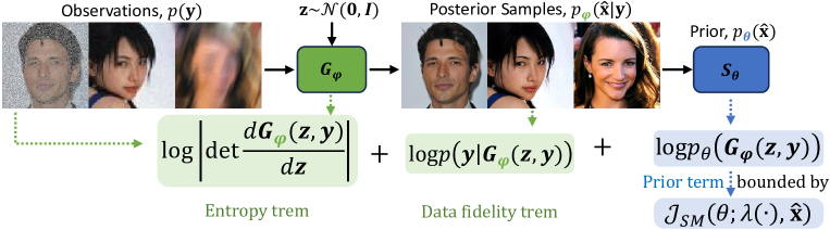
Figure 1: Overview of the FlowDiff. We aim to train a clean diffusion model, $s_{\theta}$, using only corrupted observations. To achieve this, a conditional normalizing flow, $G_{\varphi}$, is introduced to recover underlying clean images through amortized inference. The conditional normalizing flow and the diffusion model are trained jointly: the flow generates clean images for training the diffusion model, while the diffusion model provides an image prior to regularize the output of the flow. Once the two networks reach equilibrium, clean reconstructions of corrupted observations are produced, and a clean diffusion prior is learned.

3.2 Jointly optimizing score-based priors

Ideally, we adopt a clean DM pre-trained on large-scale signals as a plug-and-play prior to Eq. 6. Extensive works have focused on solving general inverse problems in this paradigm. We argue that it is feasible to train this prior jointly with the amortized inference framework. Assuming that the posterior samples are clean, we can train the score-based DM through well-established techniques.

Maximum likelihood training of score-based diffusion models Our goal is to learn the data distribution by approximating their score function $\nabla_{\mathbf{x}}\log p(\mathbf{x})$ with a neural network $\mathbf{s}_{\theta}$. In order to train $s_{\theta}(\mathbf{x},t)$,  song2019generative proposed score matching loss

$$\mathcal{J}_{SM}(\mathbf{\theta};\lambda(\cdot))=\frac{1}{2}\int_{0}^{T}\mathbb{E}_{p_{t}(\mathbf{x})}\left[\lambda(t)\|\nabla_{\mathbf{x}}\log p_{t}(\mathbf{x})-\mathbf{s}_{\theta}(\mathbf{x},t)\|_{2}^{2}\right],$$ (7)

where $\lambda(t)$ is a weighting factor, i.e. $\lambda(t)=g(t)^{2}$. Eq. 7 stands for a weighted MSE loss between $\mathbf{s}_{\theta}(\mathbf{x},t)$ and $\nabla_{\mathbf{x}}\log p_{t}(\mathbf{x})$ with a manually chosen weighting function $\lambda(t)$. During training, we ignore $\lambda(t)$ for the benefits of sample quality (and simpler to implement) ho2020denoising . Notably, the score matching loss could also serve as a data-driven regularizer during inference.

Prior probability computed through DMs By removing the Brownian motion from the reverse-time SDE in Eq. 2, that is, ignoring the stochastic term in the SDE, we can derive a probability flow ODE sampler song2020score :

$$d\mathbf{x}=\left[\mathbf{f}(\mathbf{x},t)-\frac{1}{2}g(t)^{2}\nabla_{\mathbf{x}}\log p_{t}(\mathbf{x})\right]dt.$$ (8)

song2021maximum proved that if $s_{\theta}(\mathbf{x},t)\equiv\nabla_{\mathbf{x}}\log p_{t}(\mathbf{x})$, Then $p_{\theta}^{\rm ODE}=p_{\theta}^{\rm SDE}=p_{data}$. Assuming the former equation always holds, we can compute the probability of a single image through integration:

$$\log p_{data}(\mathbf{x}) =\log p_{\theta}^{\rm ODE}(\mathbf{x})$$ (9)

$$=\log\pi(\mathbf{x}(T))+\int_{0}^{T}\nabla_{\mathbf{x}}\cdot\left[\mathbf{f}(\mathbf{x},t)-\frac{1}{2}g(t)^{2}\nabla_{\mathbf{x}}\log p_{t}(\mathbf{x})\right]dt.$$

$$=\log\pi(\mathbf{x}(T))+\int_{0}^{T}\nabla_{\mathbf{x}}\cdot\left[\mathbf{f}(\mathbf{x},t)-\frac{1}{2}g(t)^{2}s_{\theta}(\mathbf{x},t)\right]dt.$$

feng2023score has verified that a pre-trained $\mathbf{s}_{\theta}$ can serve as a powerful plug-and-play prior for inverse imaging. However, the log-probability function in Eq. 9 is computationally expensive, requiring hundreds of discrete ODE time steps to accurately compute, thus not practical to use in the training process. To reduce the computational overhead,  song2021maximum ; feng2023efficient prove that the evidence lower bound (ELBO) could approximate the performance of $p_{\theta}^{\rm ODE}$ to serve as a prior distribution. Interestingly, we find that in our setting, the score matching loss in Eq. 7 becomes a lower bound of $\log p(\mathbf{x})$ by selecting a specific weighting function $\lambda(\cdot)=g(\cdot)^{2}$, which gives us an explicit function to approximate the probability of a prior image song2021maximum :

$$-\mathbb{E}_{p(\mathbf{x})}\left[\log p_{data}(\mathbf{x})\right]=-\mathbb{E}_{p(\mathbf{x})}\left[\log p_{\theta}^{\text{SDE}}(\mathbf{x})\right]\leq\mathcal{J}_{SM}(\mathbf{\theta};g(\cdot)^{2})+C$$ (10)

Consequently, by replacing $\mathbb{E}_{p(\hat{\mathbf{x}})}\left[-\log p(\hat{\mathbf{x}})\right]$ in Eq. 6 with the upper bound in Eq. 10, we derive the loss for jointly optimizing the normalizing flow and the score-based diffusion prior.

3.3 Implementation details

Training scheme

We briefly discuss how to jointly train the normalizing flow and the diffusion model with the objective function in Eq. 6. Figure 1 illustrates our training framework. Our training loss consists of three terms: the first two terms (highlighted in green) are influenced only by the amortized inference network (i.e., conditional normalizing flow), while the third term (highlighted in blue) is influenced by both the inference network and the diffusion prior. In our joint optimization implementation, we alternate between updating the weights of the flow and the diffusion model in each training step. The flow is trained with all three terms, as defined in Eq.6, assuming the diffusion prior is fixed. Then, we fix the flow’s weights and use the posterior images sampled from the flow model to train the DM using only the third term, i.e., the score matching loss defined in Eq.7. Note that when training the DM, we remove the weighting function $\lambda(t)$ in Eq.7 for better performance, as suggested by Kingma et al. kingma2024understanding .

Model reset

Considering the joint optimization of the normalizing flow and diffusion model is highly non-convex, we often observe unstable model performance during training. Additionally, because both the normalizing flow and the diffusion prior are randomly initialized, they are initially trained with poor posterior samples, hindering optimal convergence due to memorization effects. To help the networks escape local minima, we periodically reset the weights of the normalizing flow and diffusion prior after a certain number of joint training steps.

For example, in denoising tasks, we reset the weights of the normalizing flow (amortized inference network) after 9000 joint training steps and retrain it from scratch until convergence, fixing the learned diffusion prior at the 9000th step. We then reverse the process: using the improved normalizing flow to generate better posterior samples, we retrain the diffusion model from scratch until it converges. Empirically, this model resetting strategy significantly reduces the influence of memorization effects, thereby enhancing both the amortized inference accuracy and the generative performance of the diffusion model. We also employ a similar strategy for the deblurring task.

Posterior sampling

In addition to generating posterior samples using amortized inference, the inverse problem can also be solved by leveraging the Diffusion Posterior Sampling (DPS) algorithm chung2022diffusion to sample from corrupted observations using the learned diffusion model. Specifically, we modify the reverse-time SDE from Eq. 2 into a conditional reversed process for posterior sampling:

$$\quad d\mathbf{x}=\left[\mathbf{f}(\mathbf{x},t)-g(t)^{2}\nabla_{\mathbf{x}}\log p_{t}(\mathbf{x}\mid\mathbf{y})\right]dt+g(t)d\mathbf{\overline{w}},$$ (11)

where $\mathbf{y}$ is the given observation. Using Bayes’ theorem, the conditional score function can be decomposed into:

$$\nabla_{\mathbf{x}}\log p_{t}(\mathbf{x}|\mathbf{y})=\nabla_{\mathbf{x}}\log p_{t}(\mathbf{y}\mid\mathbf{x})+\nabla_{\mathbf{x}}\log p_{t}(\mathbf{x}).$$ (12)

Here $\nabla_{\mathbf{x}}\log p_{t}(\mathbf{x})$ can be replaced by the learned score function $\mathbf{s}_{\theta}(\mathbf{x},t)$, while for $\nabla_{\mathbf{x}}\log p_{t}(\mathbf{y}\mid\mathbf{x})$ we adopt the approximation proposed by DPS chung2022diffusion :

$$p_{t}\left(\mathbf{y}\mid\mathbf{x}\right)\simeq p\left(\mathbf{y}\mid\hat{\mathbf{x}}_{0}(\mathbf{x})\right),\quad\text{where}\quad\hat{\mathbf{x}}_{0}(\mathbf{x}_{t}):=\mathbb{E}\left[\mathbf{x}_{0}\mid\mathbf{x}_{t}\right],$$ (13)

Substituting Eq.13 and Eq.12 into Eq. 11, we obtain a conditional reverse-time SDE that can reconstruct images from corrupted observations.

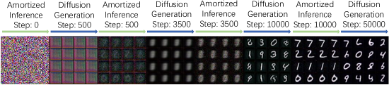
Figure 2: Training procedure of the conditional flow model and the diffusion model. We alternately report the amortized inference results from the flow model and the generative images from the diffusion model during training. The diffusion model initially captures low-frequency signals, guiding the amortized inference model. As the amortized inference improves, it produces better-quality images, further enhancing the diffusion model’s training. Eventually, both models converge to produce clean images.

4 Experiments

In this section, we first demonstrate our method on image denoising and deblurring tasks using various datasets, including MNIST, CIFAR-10, and fluorescent microscopic images of tubulins. After that, we apply the models learned by our methods to solving inverse problems. Further details on neural network architectures, training settings, and additional reconstruction and generation samples are provided in the appendix.

4.1 Experimental setting

Datasets

Our experiments are conducted on three sets of corrupted observations. First, we performed a toy experiment on denoising MNIST images corrupted by additive Gaussian noise with $\sigma=0.3$. Next, we tested our method on a deblurring task using dog images from CIFAR-10, where all images were blurred by a Gaussian kernel of size 3$\times$3 and a standard deviation of 1.5 pixels. Finally, for more realistic, higher-resolution images, we attempted to restore and learn a clean distribution from noisy microscopic images of tubulins, assuming they are corrupted by additive Gaussian noise with $\sigma=0.2$.

Evaluation metrics

We use the Frechet Inception Distance (FID) parmar2022aliased to assess the generative ability of our learned diffusion model by comparing 5000 image samples generated from it to reserved test data from the underlying true distribution. For posterior sampling results, including those from either the amortized inference network or the conditional diffusion process using the learned generative model, we compute Peak Signal-to-Noise Ratio (PSNR), Structural Similarity (SSIM), and Learned Perceptual Image Patch Similarity (LPIPS) to evaluate the image reconstruction quality.

\begin{overpic}[width=106.23477pt]{Styles/fig/flow-fig3/1-1.png} \end{overpic} \begin{overpic}[width=106.23477pt]{Styles/fig/flow-fig3/1-2.png} \end{overpic} \begin{overpic}[width=106.23477pt]{Styles/fig/flow-fig3/1-3.png} \end{overpic} \begin{overpic}[width=106.23477pt]{Styles/fig/flow-fig3/1-4.png} \end{overpic} (a) Ground Truth (b) Observations, FID=204 (c) AmbientFlow kelkar2023ambientflow , FID=147 (d) Ours, FID=149 \begin{overpic}[width=106.23477pt]{Styles/fig/flow-fig3/2-1.png} \end{overpic} \begin{overpic}[width=106.23477pt]{Styles/fig/flow-fig3/2-2.png} \end{overpic} \begin{overpic}[width=106.23477pt]{Styles/fig/flow-fig3/2-3.png} \end{overpic} \begin{overpic}[width=106.23477pt]{Styles/fig/flow-fig3/2-4.png} \end{overpic} (a) Ground Truth (b) Observations, FID=109 (c) AmbientFlow kelkar2023ambientflow , FID=272 (d) Ours, FID=209 \begin{overpic}[width=106.23477pt]{Styles/fig/flow-fig3/3-1.png} \end{overpic} \begin{overpic}[width=106.23477pt]{Styles/fig/flow-fig3/3-2.png} \end{overpic} \begin{overpic}[width=106.23477pt]{Styles/fig/flow-fig3/3-3.png} \end{overpic} \begin{overpic}[width=106.23477pt]{Styles/fig/flow-fig3/3-4.png} \end{overpic} (a) Ground Truth (b) Observations, FID=298 (c) AmbientFlow kelkar2023ambientflow , FID=295 (d) Ours, FID=210

Figure 3: Image samples from diffusion models learned from corrupted observations. The three rows show results from models trained on different datasets: noisy MNIST handwritten digits, blurred CIFAR-10 dog images, and noisy fluorescent microscope images. The learned diffusion models generate samples similar to the ground-truth images, significantly outperforming the baseline, AmbientFlow. Notably, when directly training the diffusion model using blurred images (2nd row (b)), we achieve samples with low FID scores. This is because FID mainly measures the similarity of smoothed features among image sets. However, our method (2nd row (d)) produces more reasonable and sharper dog images, despite the FID score not being superior.

Baselines

We compare our methods with three baselines that operate under the same conditions, where no clean signals are available. AmbientFlow kelkar2023ambientflow employs a similar amortized inference approach but uses a normalizing flow model kingma2018glow , instead of a diffusion model, to learn the unconditional clean distribution. AmbientDiffusion daras2023ambient learns a clean score-based prior by further corrupting the input data, rather than restoring the clean images first. SURE-Score aali2023solving combines the SURE loss stein1981estimation to implicitly regularize the weights of the learned diffusion model, enabling direct training of clean diffusion models using corrupted observations. We carefully tune the hyperparameters of all the baselines and report the best results. More information on these neural networks’ architectures and hyperparameters can be found in Appendix A.

4.2 Results

Observation Ambient Flow kelkar2023ambientflow Ours Ground Truth Observation Ambient Flow kelkar2023ambientflow Ours Ground Truth \begin{overpic}[width=52.03227pt]{Styles/fig/fig4/1-1.png} \end{overpic} \begin{overpic}[width=52.03227pt]{Styles/fig/fig4/1-2.png} \end{overpic} \begin{overpic}[width=52.03227pt]{Styles/fig/fig4/1-3.png} \end{overpic} \begin{overpic}[width=52.03227pt]{Styles/fig/fig4/1-4.png} \end{overpic} \begin{overpic}[width=52.03227pt]{Styles/fig/fig4/1-5.png} \end{overpic} \begin{overpic}[width=52.03227pt]{Styles/fig/fig4/1-6.png} \end{overpic} \begin{overpic}[width=52.03227pt]{Styles/fig/fig4/1-7.png} \end{overpic} \begin{overpic}[width=52.03227pt]{Styles/fig/fig4/1-8.png} \end{overpic} (a) Amortized Inference Results of CIFAR-10 (b) Amortized Inference Results of Tubulins

Figure 4: Amortized inference results on CIFAR-10 deblurring and microscopy imaging tasks. Our method achieves superior performance compared to AmbientFlow, because of the diffusion model’s stronger generative modeling capabilities over the flow model employed by AmbientFlow.

Observation Ambient Diffusion daras2023ambient SURE- Score aali2023solving Ambient Flow kelkar2023ambientflow Ours Ground Truth Observation Ambient Diffusion daras2023ambient SURE- Score aali2023solving Ambient Flow kelkar2023ambientflow Ours Ground Truth \begin{overpic}[width=33.82362pt]{Styles/fig/fig5/1-1.png} \end{overpic} \begin{overpic}[width=33.82362pt]{Styles/fig/fig5/1-2.png} \end{overpic} \begin{overpic}[width=33.82362pt]{Styles/fig/fig5/1-3.png} \end{overpic} \begin{overpic}[width=33.82362pt]{Styles/fig/fig5/1-4.png} \end{overpic} \begin{overpic}[width=33.82362pt]{Styles/fig/fig5/1-5.png} \end{overpic} \begin{overpic}[width=33.82362pt]{Styles/fig/fig5/1-6.png} \end{overpic} \begin{overpic}[width=33.82362pt]{Styles/fig/fig5/1-7.png} \end{overpic} \begin{overpic}[width=33.82362pt]{Styles/fig/fig5/1-8.png} \end{overpic} \begin{overpic}[width=33.82362pt]{Styles/fig/fig5/1-9.png} \end{overpic} \begin{overpic}[width=33.82362pt]{Styles/fig/fig5/1-10.png} \end{overpic} \begin{overpic}[width=33.82362pt]{Styles/fig/fig5/1-11.png} \end{overpic} \begin{overpic}[width=33.82362pt]{Styles/fig/fig5/1-12.png} \end{overpic} \begin{overpic}[width=33.82362pt]{Styles/fig/fig5/2-1.png} \end{overpic} \begin{overpic}[width=33.82362pt]{Styles/fig/fig5/2-2.png} \end{overpic} \begin{overpic}[width=33.82362pt]{Styles/fig/fig5/2-3.png} \end{overpic} \begin{overpic}[width=33.82362pt]{Styles/fig/fig5/2-4.png} \end{overpic} \begin{overpic}[width=33.82362pt]{Styles/fig/fig5/2-5.png} \end{overpic} \begin{overpic}[width=33.82362pt]{Styles/fig/fig5/2-6.png} \end{overpic} \begin{overpic}[width=33.82362pt]{Styles/fig/fig5/2-7.png} \end{overpic} \begin{overpic}[width=33.82362pt]{Styles/fig/fig5/2-8.png} \end{overpic} \begin{overpic}[width=33.82362pt]{Styles/fig/fig5/2-9.png} \end{overpic} \begin{overpic}[width=33.82362pt]{Styles/fig/fig5/2-10.png} \end{overpic} \begin{overpic}[width=33.82362pt]{Styles/fig/fig5/2-11.png} \end{overpic} \begin{overpic}[width=33.82362pt]{Styles/fig/fig5/2-12.png} \end{overpic} (a) CIFAR-10, Denoising (b) CIFAR-10, Deblurring Observation Ambient Diffusion daras2023ambient SURE- Score aali2023solving Ambient Flow kelkar2023ambientflow Ours Ground Truth Observation Ambient Diffusion daras2023ambient SURE- Score aali2023solving Ambient Flow kelkar2023ambientflow Ours Ground Truth \begin{overpic}[width=33.82362pt]{Styles/fig/fig5/3-1.png} \end{overpic} \begin{overpic}[width=33.82362pt]{Styles/fig/fig5/3-2.png} \end{overpic} \begin{overpic}[width=33.82362pt]{Styles/fig/fig5/3-3.png} \end{overpic} \begin{overpic}[width=33.82362pt]{Styles/fig/fig5/3-4.png} \end{overpic} \begin{overpic}[width=33.82362pt]{Styles/fig/fig5/3-5.png} \end{overpic} \begin{overpic}[width=33.82362pt]{Styles/fig/fig5/3-6.png} \end{overpic} \begin{overpic}[width=33.82362pt]{Styles/fig/fig5/3-7.png} \end{overpic} \begin{overpic}[width=33.82362pt]{Styles/fig/fig5/3-8.png} \end{overpic} \begin{overpic}[width=33.82362pt]{Styles/fig/fig5/3-9.png} \end{overpic} \begin{overpic}[width=33.82362pt]{Styles/fig/fig5/3-10.png} \end{overpic} \begin{overpic}[width=33.82362pt]{Styles/fig/fig5/3-11.png} \end{overpic} \begin{overpic}[width=33.82362pt]{Styles/fig/fig5/3-12.png} \end{overpic} \begin{overpic}[width=33.82362pt]{Styles/fig/fig5/4-1.png} \end{overpic} \begin{overpic}[width=33.82362pt]{Styles/fig/fig5/4-2.png} \end{overpic} \begin{overpic}[width=33.82362pt]{Styles/fig/fig5/4-3.png} \end{overpic} \begin{overpic}[width=33.82362pt]{Styles/fig/fig5/4-4.png} \end{overpic} \begin{overpic}[width=33.82362pt]{Styles/fig/fig5/4-5.png} \end{overpic} \begin{overpic}[width=33.82362pt]{Styles/fig/fig5/4-6.png} \end{overpic} \begin{overpic}[width=33.82362pt]{Styles/fig/fig5/4-7.png} \end{overpic} \begin{overpic}[width=33.82362pt]{Styles/fig/fig5/4-8.png} \end{overpic} \begin{overpic}[width=33.82362pt]{Styles/fig/fig5/4-9.png} \end{overpic} \begin{overpic}[width=33.82362pt]{Styles/fig/fig5/4-10.png} \end{overpic} \begin{overpic}[width=33.82362pt]{Styles/fig/fig5/4-11.png} \end{overpic} \begin{overpic}[width=33.82362pt]{Styles/fig/fig5/4-12.png} \end{overpic} (c) CIFAR-10, Inpainting (d) CIFAR-10, Deblurring+Denoising

Figure 5: Posterior samples from the generative model trained on blurred CIFAR-10 images. On four downstream tasks - denoising, deblurring, inpainting, and combined denoising and deblurring - our method surpasses the performance of baseline approaches including AmbientDiffusion, SURE-Score, and AmbientFlow.

Clean distributions learned from corrupted observations

Fig 3 compares the FID scores of image samples from the baseline method, AmbientFlow, and our method, FlowDiff. As shown in Fig.3, our method significantly outperforms AmbientFlow across all three tasks, learning high-quality, complex, clean image distributions from blurred or noisy observations. During training, as illustrated in Fig. 2, we observed that the diffusion model captures low-frequency signals first, providing guidance for the amortized inference model. As the amortized inference improves, it produces better-quality images, which in turn enhances the training of the diffusion model. By alternatively updating the weights of these models, the diffusion model eventually learns the distribution of the clean data. The model reset technique described in Sec. 3.3 is used in our training process.

Table 1: Amortized inference results for three different tasks. In all cases, our method produces a better flow model for amortized inference than AmbientFlow, despite using the same flow architectures. This indicates that the diffusion model in our framework provides a superior prior compared to the flow prior in AmbientFlow. The optimal results are highlighted in bold.

Tasks	Input			AmbientFlow			Ours
	PSNR$\uparrow$	SSIM$\uparrow$	LPIPS$\downarrow$	PSNR$\uparrow$	SSIM$\uparrow$	LPIPS$\downarrow$	PSNR$\uparrow$	SSIM$\uparrow$	LPIPS$\downarrow$
MNIST Denoising	13.57	0.210	0.591	21.18	0.394	0.177	20.73	0.399	0.160
CIFAR-10 Deblurring	20.91	0.582	0.182	20.38	0.704	0.199	21.97	0.787	0.135
Microscopy Imaging	14.32	0.106	0.572	16.76	0.220	0.467	18.87	0.263	0.397

Amortized inference

Fig. 4 and Table 1 present the amortized inference results, i.e., the posterior samples drawn from the conditional normalizing flow. Our method produces better reconstructed images compared to AmbientFlow. Furthermore, results show that the amortized inference models trained by our method achieve performance comparable to those trained with a clean diffusion prior, again demonstrating that our method successfully captures the underlying clean data distribution. More details can be found in Appendix C.

Table 2: Performance on downstream posterior sampling tasks using the CIFAR-10 dog images. The optimal results are highlighted in bold, and the second-best results are underlined. All metrics are computed using 128 posterior samples.

Tasks	Metrics	Input	Ambient Diffusion	SURE- Score	Ambient Flow	Ours
Denoising	PSNR $\uparrow$	14.79	21.37	19.04	14.95	21.70
	SSIM $\uparrow$	0.444	0.743	0.636	0.356	0.782
	LPIPS $\downarrow$	0.107	0.033	0.111	0.142	0.040
Deblurring	PSNR$\uparrow$	22.34	16.14	23.52	15.03	23.91
	SSIM $\uparrow$	0.724	0.761	0.829	0.305	0.880
	LPIPS$\downarrow$	0.228	0.074	0.078	0.163	0.031
Deblurring + Denoising	PSNR$\uparrow$	19.34	16.23	21.28	15.11	22.55
	SSIM $\uparrow$	0.609	0.767	0.666	0.339	0.816
	LPIPS$\downarrow$	0.044	0.062	0.122	0.137	0.037
Inpainting	PSNR $\uparrow$	13.49	20.57	21.60	13.20	22.46
	SSIM $\uparrow$	0.404	0.639	0.732	0.217	0.836
	LPIPS$\downarrow$	0.295	0.038	0.049	0.179	0.034

Posterior sampling with learned clean prior

We leverage the learned clean priors to solve various downstream computational imaging inverse problems, including inpainting, denoising, deblurring, and a combination of denoising and deblurring. Table 2 and Fig. 5 present comprehensive experiments on CIFAR-10 across all four tasks. Assuming the clean distributions are trained on blurred images as explained in Sec. 4.1, our methods significantly outperform all the baselines, including AmbientDiffusion, SURE-Score, and AmbientFlow, across all tasks.

5 Conclusion and limitation

In this work, we present FlowDiff, a framework that integrates amortized inference with state-of-the-art diffusion models to learn clean signal distributions directly from corrupted observations. Through amortized inference, our framework incorporates an additional normalizing flow kingma2018glow that generates clean images from corrupted observations. The normalizing flow is trained jointly with the DM in a variational inference framework: the normalizing flow generates clean images for training the DM, while the DM imposes an image prior to guide reasonable estimations by the normalizing flow. After training, our method provides both a diffusion prior that models a complex, high-quality clean image distribution and a normalizing flow-based amortized inference network that directly generates posterior samples from corrupted observations. We demonstrate our method through extensive experiments on various datasets and multiple computational imaging tasks. We also apply the models our method learned to solving inverse problems including denoising, deblurring, and inpainting.

However, the different learning speeds of diffusion models and normalizing flows make the joint training of the two networks sometimes unstable. Besides, normalizing flows often fail to model complex data distributions due to their limited model capacity. In the future, we plan to explore better optimization frameworks, such as alternating optimization methods like expectation-maximization, to achieve more stable training.

Appendix A Neural network architectures and hyper-parameters

We conducted all our experiments using the same neural network architectures, but slightly adjusting the number of parameters based on the complexity of the data distribution. The specific numbers are shown in Table 3. For our amortized inference model, we use the same conditional invertible network as AmbientFlow kelkar2023ambientflow and employ DDPM ho2020denoising for learning the clean distribution. To balance the learning speeds between the flow model and the diffusion model, we set the learning rate of the diffusion model to be smaller. Specifically, for the MNIST and CIFAR-10 experiments, the flow network’s learning rate is $1e-3$ and the diffusion model’s learning rate is $1e-4$. For the microscopic experiment, we train the normalizing flow with a learning rate of $2e-5$ and the diffusion model with a learning rate of $1e-5$. We use Adam kingma2014adam as the optimizer for our models. All the experiments are conducted on an NVIDIA A800 GPU workstation.

Table 3: The number of model parameters for each experiment. We adjusted the size of our models based on the complexity of data distributions as well as the resolution of input images.

	MNIST	CIFAR-10	Microscopic images of tubulins
Flow	8M	11.5M	23.9M
Diffusion	6M	35.7M	17.2M

\begin{overpic}[width=84.55907pt]{Styles/fig/flow-fig6/1-1.png} \put(15.0,86.0){{\color[rgb]{1,1,1}PSNR: 18.16}} \end{overpic} \begin{overpic}[width=84.55907pt]{Styles/fig/flow-fig6/1-2.png} \put(15.0,86.0){{\color[rgb]{1,1,1}PSNR: 20.77}} \end{overpic} \begin{overpic}[width=84.55907pt]{Styles/fig/flow-fig6/1-3.png} \put(15.0,86.0){{\color[rgb]{1,1,1}PSNR: 17.74}} \end{overpic} \begin{overpic}[width=84.55907pt]{Styles/fig/flow-fig6/1-4.png} \put(15.0,86.0){{\color[rgb]{1,1,1}PSNR: 22.87}} \end{overpic} \begin{overpic}[width=84.55907pt]{Styles/fig/flow-fig6/1-5.png} \end{overpic} \begin{overpic}[width=84.55907pt]{Styles/fig/flow-fig6/2-1.png} \put(15.0,86.0){{\color[rgb]{1,1,1}PSNR: 18.00}} \end{overpic} \begin{overpic}[width=84.55907pt]{Styles/fig/flow-fig6/2-2.png} \put(15.0,86.0){{\color[rgb]{1,1,1}PSNR: 20.38}} \end{overpic} \begin{overpic}[width=84.55907pt]{Styles/fig/flow-fig6/2-3.png} \put(15.0,86.0){{\color[rgb]{1,1,1}PSNR: 17.33}} \end{overpic} \begin{overpic}[width=84.55907pt]{Styles/fig/flow-fig6/2-4.png} \put(15.0,86.0){{\color[rgb]{1,1,1}PSNR: 22.99}} \end{overpic} \begin{overpic}[width=84.55907pt]{Styles/fig/flow-fig6/2-5.png} \end{overpic} \begin{overpic}[width=84.55907pt]{Styles/fig/flow-fig6/3-1.png} \put(15.0,86.0){{\color[rgb]{1,1,1}PSNR: 18.12}} \end{overpic} \begin{overpic}[width=84.55907pt]{Styles/fig/flow-fig6/3-2.png} \put(15.0,86.0){{\color[rgb]{1,1,1}PSNR: 20.28}} \end{overpic} \begin{overpic}[width=84.55907pt]{Styles/fig/flow-fig6/3-3.png} \put(15.0,86.0){{\color[rgb]{1,1,1}PSNR: 16.87}} \end{overpic} \begin{overpic}[width=84.55907pt]{Styles/fig/flow-fig6/3-4.png} \put(15.0,86.0){{\color[rgb]{1,1,1}PSNR: 22.63}} \end{overpic} \begin{overpic}[width=84.55907pt]{Styles/fig/flow-fig6/3-5.png} \end{overpic} \begin{overpic}[width=84.55907pt]{Styles/fig/flow-fig6/4-1.png} \put(15.0,86.0){{\color[rgb]{1,1,1}PSNR: 17.94}} \end{overpic} \begin{overpic}[width=84.55907pt]{Styles/fig/flow-fig6/4-2.png} \put(15.0,86.0){{\color[rgb]{1,1,1}PSNR: 16.01}} \end{overpic} \begin{overpic}[width=84.55907pt]{Styles/fig/flow-fig6/4-3.png} \put(15.0,86.0){{\color[rgb]{1,1,1}PSNR: 17.10}} \end{overpic} \begin{overpic}[width=84.55907pt]{Styles/fig/flow-fig6/4-4.png} \put(15.0,86.0){{\color[rgb]{1,1,1}PSNR: 22.56}} \end{overpic} \begin{overpic}[width=84.55907pt]{Styles/fig/flow-fig6/4-5.png} \end{overpic} Observations BM3D dabov2007image Ambient Flow kelkar2023ambientflow Ours Ground Truth

Figure 6: Posterior samples from the generative model trained on noisy microscopic images. On the downstream image denoising task, our approach outperforms BM3D dabov2007image and AmbientFlow kelkar2023ambientflow by effectively removing noise while preserving intricate structural details of microscopic images of tubulins.

Appendix B Additional posterior sampling results

Table 4: Performance on downstream posterior sampling tasks using MNIST and microscopic images. The optimal results are highlighted in bold.

Method	MNIST			Microscopic images of tubulins
	PSNR$\uparrow$	SSIM$\uparrow$	LPIPS$\downarrow$	PSNR$\uparrow$	SSIM$\uparrow$	LPIPS$\downarrow$
Observations	13.36	0.344	0.103	18.89	0.477	0.252
BM3D	13.57	0.427	0.088	21.28	0.542	0.073
AmbientFlow	17.67	0.476	0.047	15.35	0.120	0.537
Ours	20.97	0.618	0.053	23.33	0.687	0.111

In this section, we present additional results on posterior sampling for the denoising task using diffusion models trained on corrupted MNIST and microscopic images. Table 4 demonstrates that our method surpasses both the classical method, BM3D dabov2007image , and the deep learning baseline, AmbientFlow, in terms of PSNR and SSIM. Fig. 6 showcases the posterior samples obtained from denoising problems using generative models trained on noisy microscopic images. Our method achieves superior denoising performance on microscopic images of tubulins, preserving detailed cellular structures visually. These findings underscore the significant potential of our framework in reconstructing clean fluorescent microscopic images, particularly in scenarios where acquiring clean signals is impractical or cost-prohibitive.

Appendix C Comparison with amortized inference models trained with a clean diffusion prior

We provide an additional comparison of our method to flow models trained with clean diffusion prior. The clean diffusion priors are trained with the clean images of MNIST and CIFAR-10. As illustrated by Fig. 7 and Table 5, the performance of the amortized inference networks trained using our method achieves similar results to those trained with clean diffusion priors.

Table 5: Amortized inference results for our method and flow trained with clean diffusion prior.

Method	MNIST			CIFAR-10
	PSNR$\uparrow$	SSIM$\uparrow$	LPIPS$\downarrow$	PSNR$\uparrow$	SSIM$\uparrow$	LPIPS$\downarrow$
Observations	13.57	0.210	0.591	20.91	0.582	0.182
Clean Prior	24.61	0.482	0.064	22.37	0.787	0.117
Ours	20.73	0.399	0.160	21.97	0.787	0.135

Observation Ours Clean Prior Ground Truth Observation Ours Clean Prior Ground Truth \begin{overpic}[width=52.03227pt]{Styles/fig/fig7/1-1.png} \end{overpic} \begin{overpic}[width=52.03227pt]{Styles/fig/fig7/1-2.png} \end{overpic} \begin{overpic}[width=52.03227pt]{Styles/fig/fig7/1-3.png} \end{overpic} \begin{overpic}[width=52.03227pt]{Styles/fig/fig7/1-4.png} \end{overpic} \begin{overpic}[width=52.03227pt]{Styles/fig/fig7/1-5.png} \end{overpic} \begin{overpic}[width=52.03227pt]{Styles/fig/fig7/1-6.png} \end{overpic} \begin{overpic}[width=52.03227pt]{Styles/fig/fig7/1-7.png} \end{overpic} \begin{overpic}[width=52.03227pt]{Styles/fig/fig7/1-8.png} \end{overpic} (a) Amortized Inference Results of MNIST (b) Amortized Inference Results of CIFAR-10

Figure 7: Comparative Analysis of Amortized Inference Networks Trained by Our Method and Clean Diffusion Priors.

References

- (1) Asad Aali, Marius Arvinte, Sidharth Kumar, and Jonathan I Tamir. Solving inverse problems with score-based generative priors learned from noisy data. arXiv preprint arXiv:2305.01166, 2023.
- (2) Ashish Bora, Eric Price, and Alexandros G Dimakis. Ambientgan: Generative models from lossy measurements. In International conference on learning representations, 2018.
- (3) Charles Bouman and Ken Sauer. A generalized gaussian image model for edge-preserving map estimation. IEEE Transactions on image processing, 2(3):296–310, 1993.
- (4) Hyungjin Chung, Jeongsol Kim, Michael T Mccann, Marc L Klasky, and Jong Chul Ye. Diffusion posterior sampling for general noisy inverse problems. arXiv preprint arXiv:2209.14687, 2022.
- (5) Kostadin Dabov, Alessandro Foi, Vladimir Katkovnik, and Karen Egiazarian. Image denoising by sparse 3-d transform-domain collaborative filtering. IEEE Transactions on image processing, 16(8):2080–2095, 2007.
- (6) Giannis Daras, Kulin Shah, Yuval Dagan, Aravind Gollakota, Alexandros G. Dimakis, and Adam Klivans. Ambient diffusion: Learning clean distributions from corrupted data, 2023.
- (7) Prafulla Dhariwal and Alexander Nichol. Diffusion models beat gans on image synthesis. Advances in neural information processing systems, 34:8780–8794, 2021.
- (8) Laurent Dinh, David Krueger, and Yoshua Bengio. Nice: Non-linear independent components estimation. arXiv preprint arXiv:1410.8516, 2014.
- (9) Berthy T Feng and Katherine L Bouman. Efficient bayesian computational imaging with a surrogate score-based prior. arXiv preprint arXiv:2309.01949, 2023.
- (10) Berthy T Feng, Jamie Smith, Michael Rubinstein, Huiwen Chang, Katherine L Bouman, and William T Freeman. Score-based diffusion models as principled priors for inverse imaging. arXiv preprint arXiv:2304.11751, 2023.
- (11) Alexandros Graikos, Nikolay Malkin, Nebojsa Jojic, and Dimitris Samaras. Diffusion models as plug-and-play priors. Advances in Neural Information Processing Systems, 35:14715–14728, 2022.
- (12) Zhiye Guo, Jian Liu, Yanli Wang, Mengrui Chen, Duolin Wang, Dong Xu, and Jianlin Cheng. Diffusion models in bioinformatics and computational biology. Nature reviews bioengineering, 2(2):136–154, 2024.
- (13) Jonathan Ho, William Chan, Chitwan Saharia, Jay Whang, Ruiqi Gao, Alexey Gritsenko, Diederik P Kingma, Ben Poole, Mohammad Norouzi, David J Fleet, et al. Imagen video: High definition video generation with diffusion models. arXiv preprint arXiv:2210.02303, 2022.
- (14) Jonathan Ho, Ajay Jain, and Pieter Abbeel. Denoising diffusion probabilistic models. Advances in neural information processing systems, 33:6840–6851, 2020.
- (15) Jonathan Ho, Tim Salimans, Alexey Gritsenko, William Chan, Mohammad Norouzi, and David J Fleet. Video diffusion models. Advances in Neural Information Processing Systems, 35:8633–8646, 2022.
- (16) Lei Huang, Hengtong Zhang, Tingyang Xu, and Ka-Chun Wong. Mdm: Molecular diffusion model for 3d molecule generation. In Proceedings of the AAAI Conference on Artificial Intelligence, volume 37, pages 5105–5112, 2023.
- (17) Bahjat Kawar, Noam Elata, Tomer Michaeli, and Michael Elad. Gsure-based diffusion model training with corrupted data. arXiv preprint arXiv:2305.13128, 2023.
- (18) Bahjat Kawar, Gregory Vaksman, and Michael Elad. Snips: Solving noisy inverse problems stochastically. Advances in Neural Information Processing Systems, 34:21757–21769, 2021.
- (19) Varun A Kelkar, Rucha Deshpande, Arindam Banerjee, and Mark A Anastasio. Ambientflow: Invertible generative models from incomplete, noisy measurements. arXiv preprint arXiv:2309.04856, 2023.
- (20) Diederik Kingma and Ruiqi Gao. Understanding diffusion objectives as the elbo with simple data augmentation. Advances in Neural Information Processing Systems, 36, 2024.
- (21) Diederik P Kingma and Jimmy Ba. Adam: A method for stochastic optimization. arXiv preprint arXiv:1412.6980, 2014.
- (22) Durk P Kingma and Prafulla Dhariwal. Glow: Generative flow with invertible 1x1 convolutions. Advances in neural information processing systems, 31, 2018.
- (23) Zhifeng Kong, Wei Ping, Jiaji Huang, Kexin Zhao, and Bryan Catanzaro. Diffwave: A versatile diffusion model for audio synthesis. arXiv preprint arXiv:2009.09761, 2020.
- (24) Kazuki Kuramochi, Kazunori Akiyama, Shiro Ikeda, Fumie Tazaki, Vincent L Fish, Hung-Yi Pu, Keiichi Asada, and Mareki Honma. Superresolution interferometric imaging with sparse modeling using total squared variation: application to imaging the black hole shadow. The Astrophysical Journal, 858(1):56, 2018.
- (25) Xiang Li, John Thickstun, Ishaan Gulrajani, Percy S Liang, and Tatsunori B Hashimoto. Diffusion-lm improves controllable text generation. Advances in Neural Information Processing Systems, 35:4328–4343, 2022.
- (26) Shitong Luo and Wei Hu. Diffusion probabilistic models for 3d point cloud generation. In Proceedings of the IEEE/CVF Conference on Computer Vision and Pattern Recognition, pages 2837–2845, 2021.
- (27) Weijian Luo. A comprehensive survey on knowledge distillation of diffusion models. ArXiv, abs/2304.04262, 2023.
- (28) Kevin P Murphy. Machine learning: A probabilistic perspective (adaptive computation and machine learning series). The MIT Press: London, UK, 2018.
- (29) Eva Nogales and Sjors HW Scheres. Cryo-em: a unique tool for the visualization of macromolecular complexity. Molecular cell, 58(4):677–689, 2015.
- (30) Gaurav Parmar, Richard Zhang, and Jun-Yan Zhu. On aliased resizing and surprising subtleties in gan evaluation. In Proceedings of the IEEE/CVF Conference on Computer Vision and Pattern Recognition, pages 11410–11420, 2022.
- (31) Robin Rombach, Andreas Blattmann, Dominik Lorenz, Patrick Esser, and Björn Ommer. High-resolution image synthesis with latent diffusion models. In Proceedings of the IEEE/CVF conference on computer vision and pattern recognition, pages 10684–10695, 2022.
- (32) Jascha Sohl-Dickstein, Eric Weiss, Niru Maheswaranathan, and Surya Ganguli. Deep unsupervised learning using nonequilibrium thermodynamics. In International conference on machine learning, pages 2256–2265. PMLR, 2015.
- (33) Yang Song, Conor Durkan, Iain Murray, and Stefano Ermon. Maximum likelihood training of score-based diffusion models. Advances in neural information processing systems, 34:1415–1428, 2021.
- (34) Yang Song and Stefano Ermon. Generative modeling by estimating gradients of the data distribution. Advances in neural information processing systems, 32, 2019.
- (35) Yang Song, Liyue Shen, Lei Xing, and Stefano Ermon. Solving inverse problems in medical imaging with score-based generative models. arXiv preprint arXiv:2111.08005, 2021.
- (36) Yang Song, Jascha Sohl-Dickstein, Diederik P Kingma, Abhishek Kumar, Stefano Ermon, and Ben Poole. Score-based generative modeling through stochastic differential equations. arXiv preprint arXiv:2011.13456, 2020.
- (37) Charles M Stein. Estimation of the mean of a multivariate normal distribution. The annals of Statistics, pages 1135–1151, 1981.
- (38) He Sun and Katherine L Bouman. Deep probabilistic imaging: Uncertainty quantification and multi-modal solution characterization for computational imaging. In Proceedings of the AAAI Conference on Artificial Intelligence, volume 35, pages 2628–2637, 2021.
- (39) Junshu Tang, Tengfei Wang, Bo Zhang, Ting Zhang, Ran Yi, Lizhuang Ma, and Dong Chen. Make-it-3d: High-fidelity 3d creation from a single image with diffusion prior. In Proceedings of the IEEE/CVF International Conference on Computer Vision, pages 22819–22829, 2023.