Quantum coherence in networks
Abstract
From a quantum information perspective, verifying quantum coherence in a quantum experiment typically requires adjusting measurement settings or changing inputs. A paradigmatic example is that of a double-slit experiment, where observing the interference pattern on the screen in a series of experimental settings where one, the other, and both slits are open unambiguously proves quantum coherence. Here we show that this is not necessary by verifying quantum coherence in a network scenario without the need for inputs. We show that there exist probability distributions for joint outcomes of three parties in a triangular network with independent sources that cannot be replicated using classical resources. Furthermore, we generalize our results to -party networks and show that the discrepancy between correlations in classical and quantum networks increases with the number of parties. To this end, we derive nonlinear inequalities that are satisfied by classical correlations and find quantum states that violate them.
I Introduction
One of the main features that distinguishes quantum physics from its classical counterpart is the superposition principle, i.e., the fact that linear combinations of quantum states form another valid state. Since the early days of quantum information science, the power of coherent quantum superposition has been exploited to achieve tasks fundamentally unattainable in classical scenarios, such as secure cryptography [1], or algorithms showing an exponential advantage over their classical analogue [2, 3]. Moreover, it was more recently shown that quantum coherence of order [4, 5] and of direction of communication [6, 7, 8] prompts an exponential reduction of communication complexity, leads to two-way [9] and multi-way signaling [10] with a single quantum particle, enhances the information acquisition speed [11], and allows to access information via quantum indistinguishability [12], etc.
Detecting quantum coherence, however, requires indirect measurements that allow the observation of interference phenomena. Formally, this is due to the fact that, while classical probabilities are added up directly, quantum probabilities correspond to the modulus square of the added amplitudes. It ought to be stressed that to reveal quantum superposition of single quantum systems, for instance in a standard double-slit experiment (or, equivalently, in a Mach-Zehnder interferometer), one needs always to compare different and incompatible scenarios. Label with “0” or “1” the setup where one of the slits is open or closed, respectively. This leads to four possible configurations, “00”, “01”, “10”, or “11”, where the first (second) bit indicates the setup of the first (second) slit. The interference term is then given by [13, 14]:
| (1) |
where is the conditional probability to detect the particle at a particular location on the screen after the slits, given the configuration . For classical particles it is straightforward to show that . However, in quantum mechanics can be non-zero. This and other standard tests that demonstrate the advantage of quantum resources over their classical counterparts, such as in tests of quantum nonlocality or contextuality, require a change of measurement settings or inputs in modern game-theoretical language [15]. This is also the case in testing coherence via tuning the interferometric phase (e.g. the phase-shift in Mach-Zehnder interferometer) [16, 10].
In this letter we put forward a protocol that allows to witness quantum coherence without the need to change inputs. Motivated by the triangle network in the search of new forms of nonlocality without inputs, we notice that our setup is a single-particle modification of the triangle network which has recently been widely studied in the context of genuine network nonlocality [17, 18, 19, 20, 21]. There, in a similar fashion to what we present here, it is possible to detect Bell nonlocality without inputs at the cost of assuming independence of the sources that emit quantum particles. We show that in a three-party scenario (arranged on a triangle network) with independent sources the parties cannot return outputs which fulfill a certain probability distribution if they only use classical resources. However, this can be achieved if they exploit quantum coherence. We also derive a nonlinear inequality that separates correlations originating from classical sources from those using quantum coherence. Finally, we extend our findings to networks with an arbitrary number of parties. With extensive numerical analysis, we demonstrate that the discrepancy between classical and quantum correlations increases with the number of parties, reaching its maximum value in the asymptotic limit. Throughout the paper presentation, for the sake of simplicity, we shall assume that the particles in question are single photons. Nevertheless, an analogous calculation can be performed for fermions or distinguishable particles, with no appreciable difference.
II Triangle network for quantum coherence
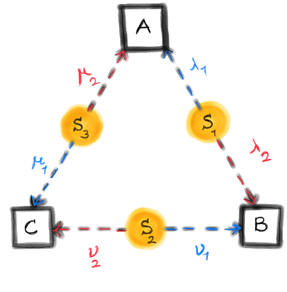
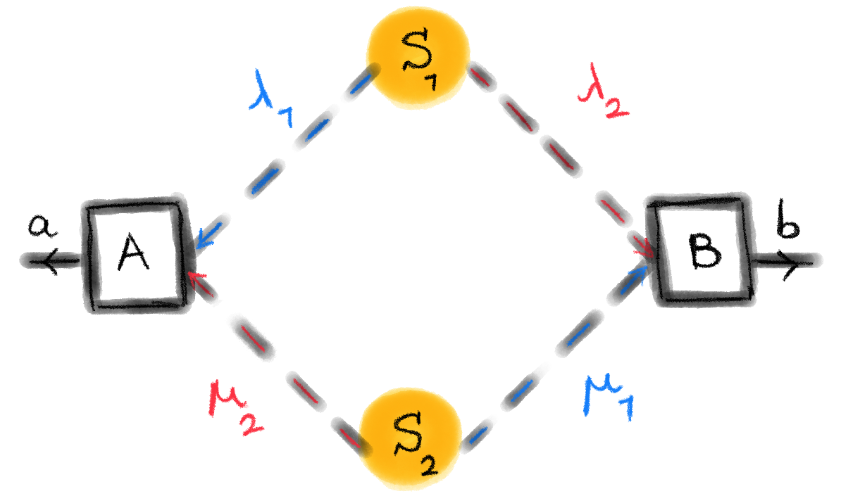
We present a protocol that can distinguish between classical scenarios and those exhibiting quantum coherence, which does not necessitate a change of settings (or inputs) between different runs. As illustrated in Fig. 1, the protocol features three parties, Alice (A), Bob (B) and Claire (C) each of whom is positioned on a different vertex of a triangle. On every edge, i.e. in between each pair of parties, there is a source –each labeled , with – of physical systems or information carriers (i.e. single-particle), which can be either classical or quantum in nature. Each source can send its corresponding particle only to the parties lying at the end of the respective edge (see Fig. 1). The parties, possibly making use of the resources that they receive from the adjacent sources, perform local operations (e.g., measurements) and each return a binary outcome, , , and , respectively. Note that A, B, and C do not change measurement setting druing the entire experiment.
The task is to return the probability distribution:
| (2) |
constrained with the following assumptions:
-
(i) Single information carriers – each source produces one information carrier (i.e., a particle) in a single experimental run;
-
(ii) Independent sources – the probability distribution associated to the emission of different sources are uncorrelated.
Note that assumption (i) can be operationally verified by a simple inspection (e.g. by measuring the path of the particle) that only a single information carrier (particle) is present in the two output beams of each source.
Furthermore, we will consider only postselected scenarios in which each party detects a single particle. This is to prevent two particles interacting at detection stations A, B or C.
II.1 Classical network
Let us now consider the most general classical network, i.e., when the information carriers can only be probabilistically directed from the source to one or the other measurement station (intuitively, this corresponds to the probabilistic distribution of trajectories of well-localized classical particles). Each independent source has a certain probability to send the particle either to the left or to the right: sends the particle to Alice with probability or to Bob with probability , to Bob with probability or to Claire with probability , and to Claire with probability or to Alice with probability (see Fig. 1). After post-selecting to a single particle per party, Alice, Bob, and Claire observe the following joint probability distribution:
| (3) |
where is the total probability for a single particle detection, and is the probability that Alice obtains outcome given that she received the particle from (). The same notation holds for Bob’s and Claire’s outcomes. This probability distribution can be understood as a classical (convex) mixture of the probabilities for the case where all sources emit particles either towards the ”left” or the ”right” from them. This postselection corresponds to the sending the three particles in a ”clockwise” or ”counterclockwise” direction within the network, respectively.
The condition in Eq. (II), stipulates that the parity of the three outcomes , , is never odd. This and Eq. (3) lead to the conjunction of the following set of conditions:
| (4) | ||||
| (5) | ||||
| (6) | ||||
| (7) | ||||
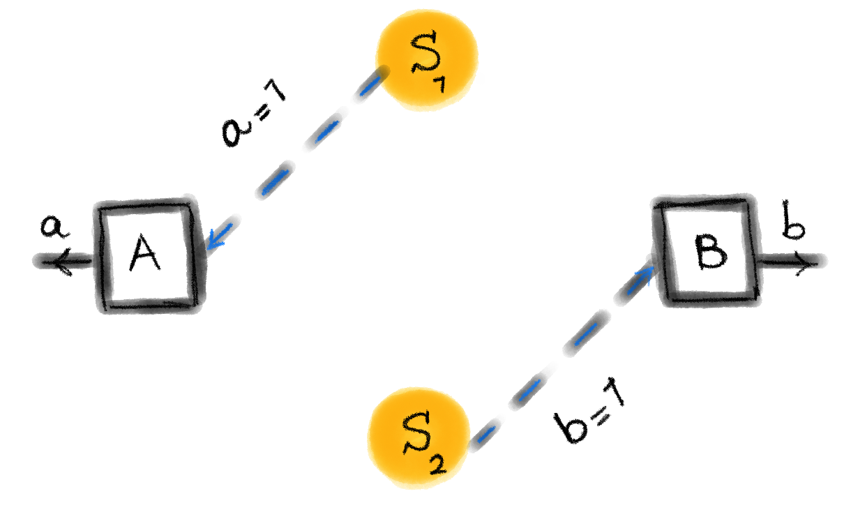
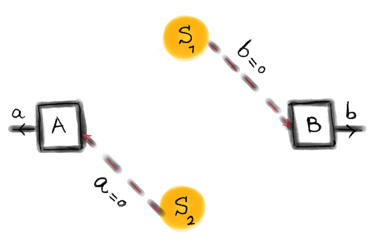
It is straightforward to demonstrate that conjunction of all above conditions (II.1-II.1) results in a contradiction with the condition given in Eq. (II). To illustrate this, let us fix the following probabilities: and . This way, condition (II.1) is satisfied. Next, we fix and to meet condition (II.1). To satisfy condition (II.1), we must have . Finally, to meet condition (II.1), we have no other choice but . This results in a contradiction with Eq.(II), as both and , leading to and . Using the same logic, one can disregard other combinations with zero probabilities that satisfy conditions (II.1-II.1).
This proves that classical networks are incompatible with the condition (II).
II.2 Quantum network
In Fig. 2, we depict a three-party quantum network 111For the sake of completeness, we demonstrate in Appendix A that no two-party scenario can distinguish between correlations originating from classical sources and those exhibiting quantum coherence. where each pair of parties shares an independent source of single quantum particles that can however be prepared in coherent superposition of both paths leading to the adjacent parties. The initial state is thus represented as:
| (8) |
where (resp. ) is the bosonic creator operator of the mode leading to Alice (resp. Bob) of the source , acting on the vacuum state . The same notation holds for the other sources and .
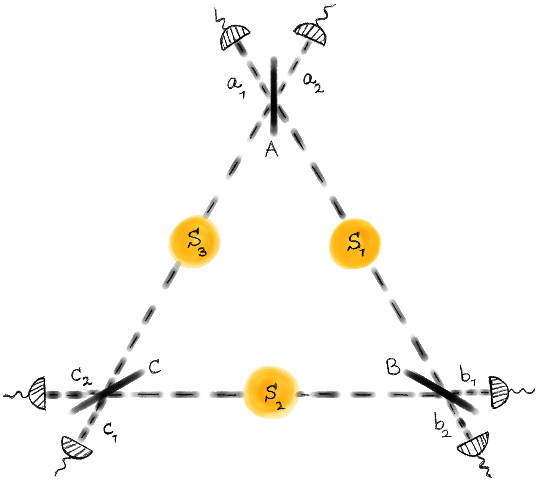
Upon crossing the paths through beam-splitters as in Fig. 2, we obtain:
| (9) |
Where and are the creation operators of bosonic modes created after the beam splitter at Alice’s station, on the left () and right () sides of the beam splitter, respectively. Similarly, and denote corresponding creation operators at Bob’s and Clair’s stations. After postselecting one particle per station, we obtain the following state:
| (10) |
This leads to the probability distribution:
| (11) |
This matches the condition given in Eq. (II).
III An inequality to test coherence without settings
The protocol presented in the previous sections shows that the use of quantum coherence can produce probability distributions not achievable with classical networks, even without involvement of settings, unlike normal interference experiments. An interesting question arises, if classical and quantum sets of probability distributions can be separated by inequalities, similarly to Bell’s inequalities. In the appendix B we show that there is no such linear inequality to distinguish classical set from quantum one due to the following reasons: the classical set is non convex, and it contains all vertices of the logical polytope. Therefore, here we use a nonlinear inequality to distinguish classical correlations from genuine quantum correlations (in network nonlocality this is a well-known problem [19]). We study the three-party case introduced above in detail and discuss the generalization to -parties in the next section.
For three parties, the non-linear expression is as follows:
| (12) |
By substituting the postselected classical three-party probability distribution as:
| (13) | ||||
| (14) |
into and maximizing numerically over all possible values for , , , , , , and , one obtains . The bound can be achieved when the probability of any pair of the following outcomes is . For instance, , which occurs when and and . However, the quantum probability distribution, as expressed in Eq. (11), yields .
IV Generalization to n-party
In the general case of -party network the task for both classical and quantum networks is to return the following probability distribution:
| (15) |
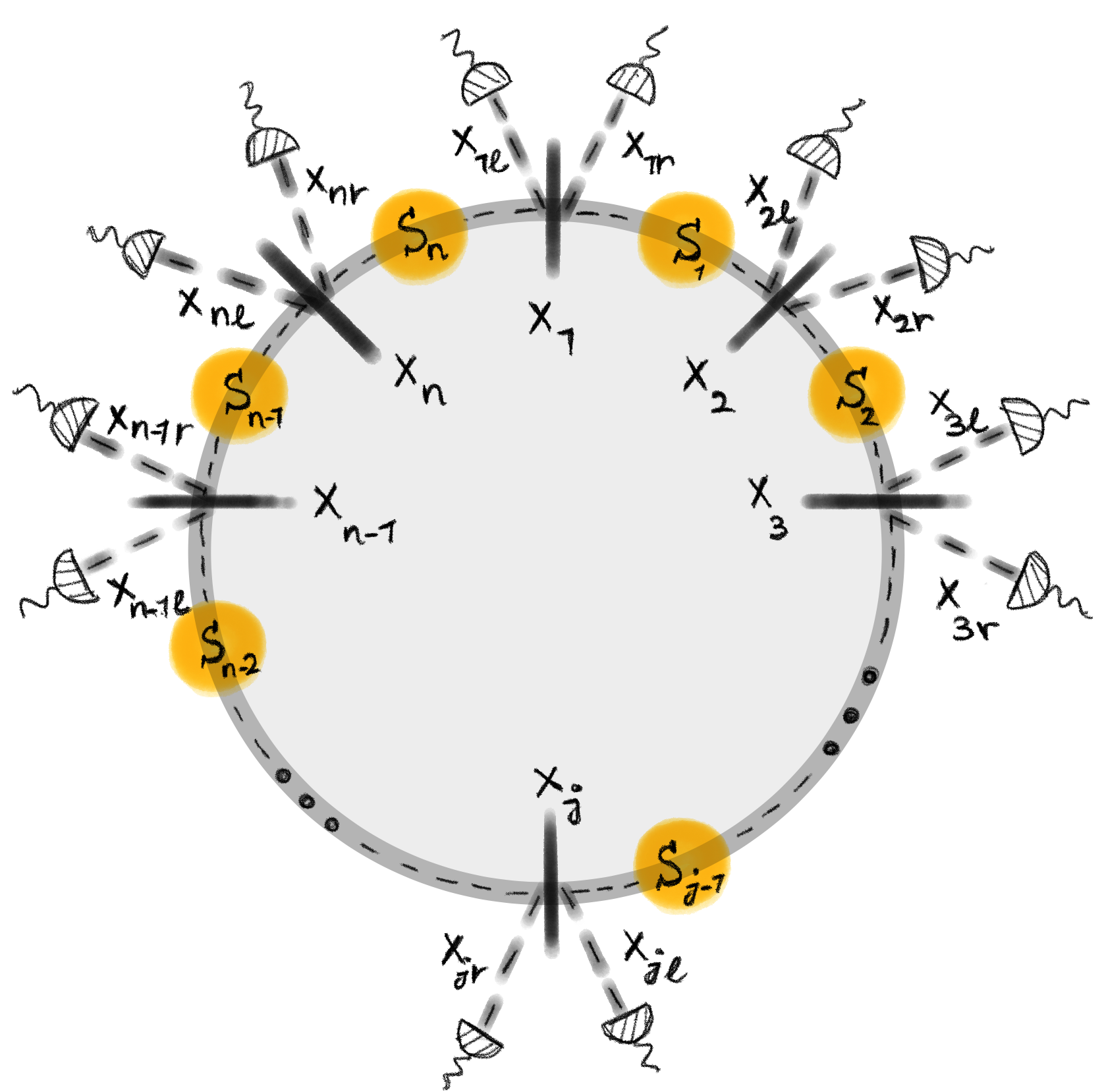
Before studying the classical case, we shall first calculate the quantum correlations. Consider -parties positioned on a -partite ring network such that neighboring parties share a single-particle source, as depicted in Fig. 3. The input state can be expressed as follows:
| (16) |
After passing through beam splitters, the state becomes:
| (17) |
where and are the bosonic creation operators of modes at the -th station, after the beam splitter, on the left and right sides, respectively. Applying post-selection on the one particle per party subspace yields:
| (18) |
Where is the normalisation factor. It is evident that the only non-zero terms are those with an even number of , where , all appearing with the same probability .
On the other hand, the classical probability can be expressed as:
| (19) |
where is the probability of particles being distributed clockwise, and () is the probability that th station outcomes given that the particles are sent in clockwise (counterclockwise) direction. This represents a convex mixture of two product distributions and thus cannot satisfy the generalized condition for given in Eq. (15).
IV.1 Generalization of the inequality to parties
Given the figure of merit in Eq. (12), a straightforward generalization of (12) becomes as follows:
| (20) |
The first summation is taken over all different vector pairs and of length with the parity of the components of both and being zero. The second summation is taken over all different vector pairs and of length with the parity of the components of both and being one. One can observe that the logical maximum of , achieved with quantum resources (Eq. (16)), is given by
| (21) |
We obtained classical bound by substituting (Eq. (IV)) into the expression for and performing extensive numerical optimization. For all tested values of , we consistently obtained . Consequently, we conjecture that for all . This result implies that the discrepancy between quantum and classical correlations increases with the number of parties, reaching a maximum value of in the limit as approaches infinity.
V Conclusions
The benefits of our investigation are twofold. Firstly, from a foundational perspective, our results provide novel insights into the understanding of quantum interference phenomena from a new angle that extends beyond standard tests. In this context, it will be interesting to see how our findings align with recent research [22, 23] on simulating quantum interference using classical stochastic fields. Secondly, our results have implications for studying quantum interference as a resource in information processing within quantum networks. There are numerous possibilities for developing novel protocols based on quantum coherence, such as scenarios with multiple senders and a single receiver, like in coherence-based multiple access channels [24], or development of cryptographic primitives based on single quantum particles [25].
VI Acknowledgements
We thank Časlav Brukner, Nicolas Gisin, Sebastian Horvat, and Sadra Boreiri for useful discussions. This research was funded in whole, or in part, by the Austrian Science Fund [10.55776/P36994] and [10.55776/COE1] and the European Union – NextGenerationEU. For open access purposes, the author(s) has applied a CC BY public copyright license to any author accepted manuscript version arising from this submission. This research was supported by the FWF (Austrian Science Fund) through an Erwin Schrödinger Fellowship (Project J 4699)
References
- Bennett and Brassard [2014] C. H. Bennett and G. Brassard, Quantum cryptography: public key distribution and coin tossing., Theor. Comput. Sci. 560, 7 (2014).
- Deutsch and Jozsa [1992] D. Deutsch and R. Jozsa, Rapid solution of problems by quantum computation, Proceedings of the Royal Society of London. Series A: Mathematical and Physical Sciences 439, 553 (1992).
- Shor [1994] P. W. Shor, Algorithms for quantum computation: Discrete logarithms and factoring, in Proceedings 35th annual symposium on foundations of computer science (1994) pp. 124–134.
- Feix et al. [2015] A. Feix, M. Araújo, and Č. Brukner, Quantum superposition of the order of parties as a communication resource, Physical Review A 92, 052326 (2015).
- Jia and Costa [2019] D. Jia and F. Costa, Causal order as a resource for quantum communication, arXiv preprint arXiv:1901.09159 (2019).
- Allard Guérin et al. [2016] P. Allard Guérin, A. Feix, M. Araújo, and Č. Brukner, Exponential communication complexity advantage from quantum superposition of the direction of communication, Phys. Rev. Lett. 117, 100502 (2016).
- Chiribella et al. [2013] G. Chiribella, G. M. D’Ariano, P. Perinotti, and B. Valiron, Quantum computations without definite causal structure, Physical Review A 88, 022318 (2013).
- Chiribella et al. [2018] G. Chiribella, M. Banik, S. S. Bhattacharya, T. Guha, M. Alimuddin, A. Roy, S. Saha, S. Agrawal, and G. Kar, Indefinite causal order enables perfect quantum communication with zero capacity channel, arXiv preprint arXiv:1810.10457 (2018).
- Del Santo and Dakić [2018] F. Del Santo and B. Dakić, Two-way communication with a single quantum particle, Phys. Rev. Lett. 120, 060503 (2018).
- Horvat and Dakić [2021a] S. Horvat and B. Dakić, Interference as an information-theoretic game, Quantum 5, 404 (2021a).
- Horvat and Dakić [2021b] S. Horvat and B. Dakić, Quantum enhancement to information acquisition speed, New Journal of Physics 23, 033008 (2021b).
- Horvat and Dakić [2023] S. Horvat and B. Dakić, Accessing inaccessible information via quantum indistinguishability, New Journal of Physics 25, 113008 (2023).
- Dakić et al. [2014] B. Dakić, T. Paterek, and Č. Brukner, Density cubes and higher-order interference theories, New Journal of Physics 16, 023028 (2014).
- Sorkin [1994] R. D. Sorkin, Quantum mechanics as quantum measure theory, Modern Physics Letters A 09, 3119 (1994).
- Brunner et al. [2014] N. Brunner, D. Cavalcanti, S. Pironio, V. Scarani, and S. Wehner, Bell nonlocality, Reviews of modern physics 86 (2014).
- Del Santo and Dakić [2020] F. Del Santo and B. Dakić, Coherence equality and communication in a quantum superposition, Physical Review Letters 124, 190501 (2020).
- Renou et al. [2019] M.-O. Renou, E. Bäumer, S. Boreiri, N. Brunner, N. Gisin, and S. Beigi, Genuine quantum nonlocality in the triangle network, Physical review letters 123, 140401 (2019).
- Boreiri et al. [2023a] S. Boreiri, A. Girardin, B. Ulu, P. Lipka-Bartosik, N. Brunner, and P. Sekatski, Towards a minimal example of quantum nonlocality without inputs, Physical Review A 107, 062413 (2023a).
- Tavakoli et al. [2022] A. Tavakoli, A. Pozas-Kerstjens, M.-X. Luo, and M.-O. Renou, Bell nonlocality in networks, Reports on Progress in Physics 85, 056001 (2022).
- Sekatski et al. [2023] P. Sekatski, S. Boreiri, and N. Brunner, Partial self-testing and randomness certification in the triangle network, Physical Review Letters 131, 100201 (2023).
- Boreiri et al. [2023b] S. Boreiri, B. Ulu, N. Brunner, and P. Sekatski, Noise-robust proofs of quantum network nonlocality, arXiv preprint arXiv:2311.02182 (2023b).
- Catani et al. [2023a] L. Catani, M. Leifer, D. Schmid, and R. W. Spekkens, Why interference phenomena do not capture the essence of quantum theory, Quantum 7, 1119 (2023a).
- Catani et al. [2023b] L. Catani, M. Leifer, G. Scala, D. Schmid, and R. W. Spekkens, Aspects of the phenomenology of interference that are genuinely nonclassical, Physical Review A 108, 022207 (2023b).
- Zhang et al. [2022] Y. Zhang, X. Chen, and E. Chitambar, Building multiple access channels with a single particle, Quantum 6, 653 (2022).
- Massa et al. [2022] F. Massa, P. Yadav, A. Moqanaki, W. O. Krawec, P. Mateus, N. Paunković, A. Souto, and P. Walther, Experimental semi-quantum key distribution with classical users, Quantum 6, 819 (2022).
VII Appendix A – Bipartite case with no quantum advantage
VII.1 Quantum case
In the scenario illustrated in Fig. 4, Alice and Bob share two independent one-particle sources, labeled as and . To prevent interactions between particles from different sources at the beam splitters, we selectively focus on the subspace where each party receives only one particle. Following the beam splitters, Alice and Bob conduct measurements to determine the position of the particle.
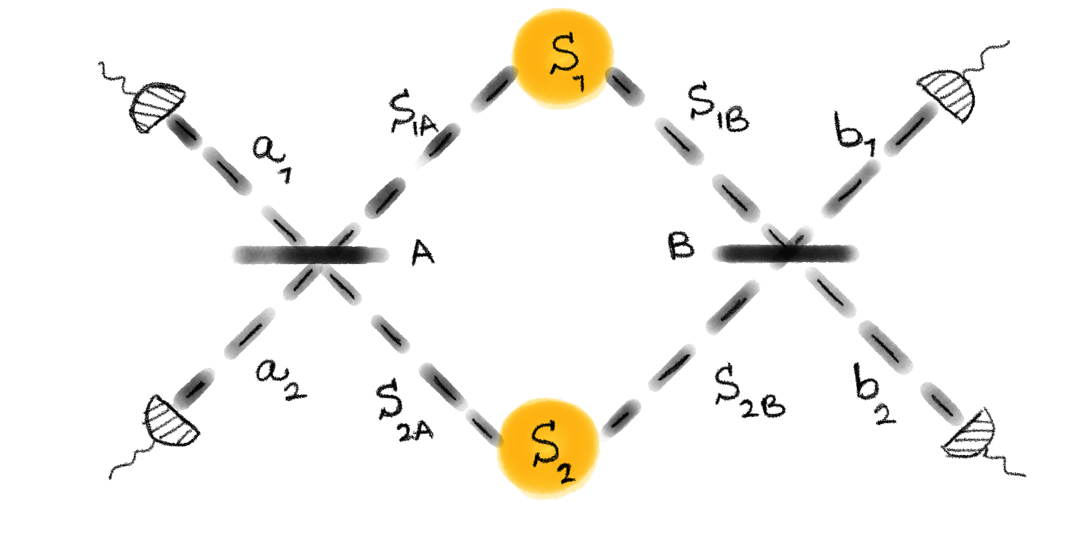
The input state can be expressed as:
| (22) |
After the beam splitter, the state becomes:
| (23) |
Applying post-selection on the subspace where each party has one particle leads to:
| (24) |
This state features a perfect correlation between the outcomes of Alice and Bob.
VII.2 Classical case
In the classical scenario, illustrated in Fig. 5, very similar to later quantum case, Alice and Bob share two independent one-particle sources, labeled and . Each particle is sent from () to Alice with probability () or to Bob with probability (). To prevent any interaction between particles from different sources that could alter their hidden variables, we select the subspace where each party receives only one particle. Throughout the experiment, Alice and Bob perform fixed measurements, yielding outcomes and , respectively.
The joint probability of Alice and Bob’s outcomes is given by:
| (25) |
Here, represents the probability of having one particle per party, and is the probability that Alice obtains result , given that the particle came from . Assuming perfect correlations such that , and , the following conditions arise:
Among these, only the combinations of and with result in correct marginals takes from state 24. For a diagrammatic solution, refer to Fig. 6.
In analogy to the three-party inequality introduced in Eq.(12) in the main text, here we introduce the nonlinear inequality for two parties as following
| (27) |
The joint classical probability distribution (see Eq. (25)) can be represented as
| (28) |
Here, represents the probability of particles being distributed among the parties in a clockwise direction and () is the probability that Alice measures outcome given that particles has been distributed in the clockwise (counter clockwise) direction. The maximum value of can be achieved through perfect correlation, a condition achievable in two-party classical networks. We conclude that perfect correlations between the outcomes of Alice and Bob can be achieved by both classical and quantum networks. This is expected because all the hidden variables from both sources are available at each measurement station, thus negating any independence condition in the situation of two-party network.
VIII Appendix B – Properties of the Classical Set
The classical subset of joint probability distributions with three variables is defined by:
| (29) | ||||
where is a probability (i.e., ), and are all valid probability distributions over the binary variables .
To check whether the set is convex or not, we assume and are elements of the classical subset. Next we need to check whether , where is a probability, can be written as a convex mixture of two three-variable product distributions. It is easy to show that this is impossible, which proves that the classical set is non-convex. The second property of the classical subset we are interested in is whether it contains all vertices of the logical polytope of three-variable probability distributions. The vertices correspond to extreme cases where for specific values of , and for . These extreme cases can be attained by setting , , , and . Therefore, the classical subset contains all vertices of the logical polytope of three-variable probability distributions. As a result, the only hyperplanes that intersect the classical subset are the facets of the logical polytope. Therefore, there is no hyperplane that can distinguish classical correlations from quantum correlations.