Chaos and integrability in triangular billiards

Abstract

We characterize quantum dynamics in triangular billiards in terms of five properties: (1) the level spacing ratio (LSR), (2) spectral complexity (SC), (3) Lanczos coefficient variance, (4) energy eigenstate localisation in the Krylov basis, and (5) dynamical growth of spread complexity. The billiards we study are classified as integrable, pseudointegrable or non-integrable, depending on their internal angles which determine properties of classical trajectories and associated quantum spectral statistics. A consistent picture emerges when transitioning from integrable to non-integrable triangles: (1) LSRs increase; (2) spectral complexity growth slows down; (3) Lanczos coefficient variances decrease; (4) energy eigenstates delocalize in the Krylov basis; and (5) spread complexity increases, displaying a peak prior to a plateau instead of recurrences. Pseudo-integrable triangles deviate by a small amount in these charactertistics from non-integrable ones, which in turn approximate models from the Gaussian Orthogonal Ensemble (GOE). Isosceles pseudointegrable and non-integrable triangles have independent sectors that are symmetric and antisymmetric under a reflection symmetry. These sectors separately reproduce characteristics of the GOE, even though the combined system approximates characteristics expected from integrable theories with Poisson distributed spectra.

1 Introduction

Chaos and integrability remain poorly understood in quantum systems. They are primarily characterized via spectral statistics: maximally chaotic systems are believed to contain level spacing correlations matching those of random matrix ensembles, while fully integrable systems have uncorrelated Poisson spectra Bohigas:1983er ; Berry:1985semiclassical ; Muller:2004semiclassical ; Haake2010 ; Dyson1972 ; Guhr:1997ve ; Lozej2022 . However, many quantum systems show behaviour somewhere between integrability and maximal chaos, and we do not understand how to precisely quantify and characterize them. Some information about the early dynamics is available in out-of-time-ordered correlators (OTOCs), which show Lyapunov-like growth for general chaotic systems, with a bound on this growth controlled by unitarity Maldacena_2016 ; Garc_a_Mata_2023 . Here, we apply a new tool in the study of quantum dynamics – spread complexity Balasubramanian:2022tpr – to characterize differences between integrable, chaotic, and an intermediate “pseudo-integrable” quantum dynamics RICHENS1981495 ; Jain_2017 .

To this end, we study systems in which these three types of dynamics are accessed by changing a few parameters: triangular quantum billiards RICHENS1981495 . In the classical billiards, a free particle bounces elastically off enclosure walls; quantum mechanically sep-ergodic-hierarchy ; Ott2002 ; PhysRevResearch.5.033126 ; Jha2014 ; PhysRevE.50.2355 ; Samajdar_2014 ; Samajdar_2018 ; Harish_1996 ; Jain_2017 the dynamics are determined by the two-dimensional Schrödinger equation with vanishing potential inside a triangular boundary where the potential diverges. Triangular billiards are not strongly chaotic – their classical Lyapunov exponent is zero because initially close trajectories separate linearly over time, and the Kolmogorov-Sinai entropy vanishes Jain_2017 ; PhysRevA.42.3170 ; MOUDGALYA201582 ; Lozej2022 . Nevertheless, these systems can exhibit ergodic and mixing behaviour PhysRevE.109.014224 ; N_Chernov_1998 . The degree of integrability/chaos is controlled by the internal angles. For example, the equilateral triangle is classically integrable – the motion can be solved by quadratures in terms of constants of motion. Generic triangles with rational angles are pseudo-integrable – beams of trajectories split at triangle vertices so that no global coordinate transformation produces momenta that are constants of motion RICHENS1981495 , while the quantum spectra show level repulsion characteristic of chaos, despite an exponential tail in the level spacing distribution characteristic of integrability Lozej:2024tpt . Meanwhile, triangles with irrational angles show mixing dynamics and have spectral statistics resembling matrices drawn from the Gaussian Orthogonal Ensemble (GOE) Lozej2022 . The symmetry of the triangle, e.g., whether it is isosceles or right-angled, also affects dynamics. Sec. 2 reviews the theory of triangular billiards and tabulates the integrable, pseudo-integrable and non-integrable triangles that we study.

In general, chaos leads to spectral correlations, while integrable theories have uncorrelated spectra. The authors of Iliesiu:2021ari proposed an integral transform of spectral density correlations as a notion of “spectral complexity” which has been used to study the stadium billard camargo2023spectral . Thus, in Sec. 3, we discuss spectral properties – level spacing ratio (LSR), spectral form factor (SFF), and spectral complexity (SC) Iliesiu:2021ari – and compare with analytical results for Poisson and GOE spectra. Generic pseudo-integrable and non-integrable triangles have level spacings and LSRs resembling the GOE, consistently with Lozej2022 ; Lozej:2024tpt , despite deviations due to numerical Hilbert space truncation and scarring. Symmetry causes larger deviations – isosceles pseudo-integrable and non-integrable triangles display Poisson-like LSRs, because eigenvalues of states even or odd under the triangles’ reflection symmetry are uncorrelated, although these sectors separately display GOE-like statistics. Right triangles show harder to characterise deviations from GOE behaviour. Finally, integrable triangles have lower-than-Poisson LSRs partly because of spectral degeneracies. We show analytically that late time spectral complexity grows linearly for non-degenerate Poisson spectra while GOE spectra show logarithmic growth, with eventual saturation if the Hilbert space is finite-dimensional. Meanwhile, energy level degeneracies lead to quadratic spectral complexity growth. Consistently, we find that the late time SC of integrable triangles, which have substantial spectral degeneracies, shows quadratic growth, while generic pseudo-integrable and non-integrable triangles exhibit logarithmic behaviour with eventual saturation. Isosceles pseudo-integrable and non-integrable triangles show linear SC growth close to the Poisson result, but the symmetric and anti-symmetric sectors deviate strongly, reflecting both the overall Poisson-like spectral character and GOE-like structure of individual sectors.

Chaos should scramble information Sekino:2008scramblers and spread operators Roberts:2014localized ; Roberts:2018operator faster than integrable dynamics. The authors of Parker:2018a proposed a measure of operator spread showing universal behaviour at early times Parker:2018a ; Kar:2021nbm ; Caputa:2021sib ; Dymarsky:2021bjq ; Barbon:2019on ; Avdoshkin:2019euclidean ; Jian:2020qpp ; Nandy:2024htc and carrying signatures of late time chaos Rabinovici:2020operator ; Dymarsky:2019quantum ; Rabinovici:2021qqt ; Rabinovici:2022beu . We also expect chaos will be more effective than integrable dynamics at transporting generic initial states throughout the Hilbert space. The authors of Balasubramanian:2022tpr proposed “spread complexity” to quantify this transport. Briefly, the idea is to measure the breadth of support of the wavefunction in a unique minimizing basis known as the Krylov basis. In this basis, the Hamiltonian is tridiagonalized, and, for Random Matrix Theories which model maximal chaos, the density of states analytically determines the tridiagonal coefficients, also called Lanczos coefficients Balasubramanian:2022dnj ; Balasubramanian:2023kwd . The temporal variation of spread complexity quantifies information spreading and chaos in quantum systems Erdmenger:2023wjg ; Balasubramanian:2023kwd .

Thus, in Sec. 4, we compare spread complexities of integrable, pseudo-integrable, and chaotic triangular billiards starting from initial states uniformly spread across the energy eigenbasis. We show that the variance of the Lanczos coefficients, i.e., non-zero entries of the tri-diagonalized Hamiltonian, is highest for integrable triangles, followed by isosceles pseudo-integrable and non-integrable triangles, and lowest for the generic triangles. The Lanczos coefficient variances turn out to be inversely related to the LSR, thus relating spread complexity to the spectral properties in Sec. 3. In the Krylov basis, every Hamiltonian describes a one-dimensional chain with hopping probabilities set by the Lanczos coefficients (see Balasubramanian:2022tpr for a discussion in the context of spread complexity). Hence Lanczos coefficient variances effectively correspond to disorder in the Krylov chain transition elements. The large Lanczos coefficient fluctuations in integrable and symmetric billiards have a consequence – localisation of the energy basis in the Krylov space as measured by the inverse participation ratio. The localisation is highest for integrable triangles, followed by pseudo-integrable and non-integrable isosceles triangles, pseudo-integrable and non-integrable right triangles, and generic triangles. For integrable triangles, spread complexity grows, saturates, and then displays recurrences. For the other triangles, the spread complexity reaches a plateau at late times after initial growth and fluctuations. Isosceles triangles exhibit slower initial growth, and do not show the complexity peak preceding a slope down to saturation that is characteristic for chaotic theories Balasubramanian:2022tpr , and is associated with classical Lyapunov exponents Hashimoto:2023swv . Restricting to the symmetric or anti-symmetric sectors in isosceles triangles reveals chaotic behaviour similar to generic triangles. This distinction is amplified in the higher moments of spread complexity.

We conclude in Sec. 5 by discussing future directions.

Note added.

While this article was being prepared, camargo2024spread appeared, using Krylov and spectral complexity to explore integrable and chaotic XXZ spin chains.

2 Setup of the billiards

In a classical billiard, a frictionless particle travels within a bounded region, undergoing elastic collision at the edges. In a quantum billiard, the wave function of a free quantum particle evolves within a two-dimensional box with an infinite barrier at the boundaries.

We numerically solve the Schrödinger equation for a quantum billiard

$$-\nabla^{2}\psi_{j}=\mathcal{E}_{j}\psi_{j},\quad j=0,1,2,\cdots$$ (1)

with Dirichlet boundary conditions $\psi_{j}(x_{\partial})=0$ at points $x_{\partial}$ on the boundary of a triangluar region. Without loss of generality, we take the particle mass to be $m=\frac{1}{2}$, set $\hbar=1$, and constrain every triangle to unit area. For each billiard we calculate the lowest $D_{0}=1000$ energy levels $\left\{\mathcal{E}_{j}\right\}_{j=0}^{D_{0}-1}$, and also separately for the symmetric and antisymmetric sectors of isosceles triangles, which are isolated by a reflection symmetry.

2.1 Choice of triangles: topology and ergodicity of classical motion

The shape of a triangular billiard determines the phase space of a classical particle moving within it, and whether the trajectories realize integrable, so-called “pseudo-integrable”, or chaotic dynamics sep-ergodic-hierarchy ; Ott2002 ; Jain_2017 ; PhysRevResearch.5.033126 . The phase space for particle motion within a two-dimensional billiard can be represented by coordinates $q=(x,y)$ and motion direction, $\theta$, because the magnitude of the momentum is conserved. When the trajectory encounters a boundary, the particle reflects Zemlyakov1975 ; RICHENS1981495 . It is convenient to represent this process by replicating the enclosure, sewing the replica at the corresponding boundary, and continuing the trajectory into the replica. If the enclosed angles of the triangle are rational fractions of $\pi$, the particle’s trajectory traverses a finite number of such sheets Zemlyakov1975 ; RICHENS1981495 ; Jain_2017 before recurring. The continuous surface produced by mirroring and attaching the traversed triangles is called the translation surface (alternatively the invariant surface RICHENS1981495 ). Since the number of traversed sheets and the enclosure size are finite for rational billiards, the translation surface will be compact by construction.

For a triangle with rational internal angles $\{\frac{p_{1}}{q_{1}},\frac{p_{2}}{q_{2}},\frac{p_{3}}{q_{3}}\}$, with $p_{i},q_{i}\in Z^{+}$ and relatively prime, the genus of the translation surface is Zemlyakov1975 :

$$g=1+\frac{\mathcal{N}}{2}\sum_{i}\left(\frac{p_{i}-1}{q_{i}}\right)$$ (2)

Here, $\mathcal{N}$ is the lowest common multiple of the $q_{i}$, and denotes the number of sheets necessary to construct the translation surface. Triangles compactifying to genus one have classically integrable dynamics according Arnold’s criterion – there are $n$ constants of motion for $n$ degrees of freedom, so dynamics restricts to an $n$-torus and can be solved by quadratures Arnold1989 ; Arnold1989 ; RICHENS1981495 . Triangles compactifying to a finite genus greater than one are said to be pseudo-integrable because, despite conservation of momentum in the replicated and sewn billiard, and contrary to the expectation from Arnold Arnold1989 , the phase space dynamics is restricted a higher genus two-dimensional surface RICHENS1981495 . This non-integrability arises because beams of trajectories intersecting some vertices of the triangle become separated into different handles of the replicated geometry RICHENS1981495 . Finally, if any internal angle is irrational, the translation surface has an infinite genus and is homeomorphic to the Loch Ness Monster, a non-compact, orientable, infinite genus surface with one end (a single-component ideal boundary) Valdez2009 . Motion in these irrational triangles is not integrable and shows signatures of chaos like level repulsion Lozej2022 even though nearby trajectories separate linearly (vanishing Lyapunov exponent). We consider triangles from all three classes (Table 1).

	g	Isosceles	Right	General
I	$1$	$\{\frac{1}{3},\frac{1}{3},\frac{1}{3}\}_{1}$, $\{\frac{1}{2},\frac{1}{4},\frac{1}{4}\}_{2}$	$\{\frac{1}{2},\frac{1}{3},\frac{1}{6}\}_{3}$	—
	$2$	$\{\frac{2}{5},\frac{2}{5},\frac{1}{5}\}_{4}$, $\{\frac{1}{5},\frac{1}{5},\frac{3}{5}\}_{5}$	$\{\frac{3}{8},\frac{1}{8},\frac{1}{2}\}_{6}$, $\{\frac{2}{5},\frac{1}{10},\frac{1}{2}\}_{7}$	—
	$3$	$\{\frac{3}{7},\frac{3}{7},\frac{1}{7}\}_{8}$	$\{\frac{5}{12},\frac{1}{12},\frac{1}{2}\}_{9}$	$\{\frac{1}{3},\frac{1}{4},\frac{5}{12}\}_{10}$
PI	$4$	$\{\frac{1}{9},\frac{4}{9},\frac{4}{9}\}_{11}$	$\{\frac{4}{9},\frac{1}{18},\frac{1}{2}\}_{12}$	$\{\frac{1}{4},\frac{1}{6},\frac{7}{12}\}_{13}$
	$5$	$\{\frac{5}{11},\frac{5}{11},\frac{1}{11}\}_{14}$	$\{\frac{9}{20},\frac{1}{20},\frac{1}{2}\}_{15}$	$\{\frac{4}{15},\frac{1}{15},\frac{2}{3}\}_{16}$
	$6$	$\{\frac{6}{13},\frac{6}{13},\frac{1}{13}\}_{17}$	$\{\frac{11}{24},\frac{1}{24},\frac{1}{2}\}_{18}$	$\{\frac{5}{16},\frac{7}{16},\frac{1}{4}\}_{19}$
NI	$\infty$	—	$\{\frac{(-1+\sqrt{5})}{8},\frac{(5-\sqrt{5})}{8},\frac{1}{2}\}_{20}$,	$\{\frac{(3-\sqrt{5})}{5},\frac{3}{5},\frac{(-1+\sqrt{5})}{5}\}_{22}$,
			$\{\frac{(6-\sqrt{5})}{8},\frac{(-2+\sqrt{5})}{8},\frac{1}{2}\}_{21}$	$\{\frac{(-2+\sqrt{5})}{8},\frac{3}{4},\frac{(4-\sqrt{5})}{8}\}_{23}$
NI	$\infty$	$\{\frac{1}{4\sqrt{2}},\frac{1}{4\sqrt{2}},\frac{(-4+\sqrt{2})}{4}\}_{24}$	—	$\{\frac{(1+\sqrt{2})(3-\sqrt{5})}{4(3+\sqrt{2})},\frac{(1+\sqrt{5})}{4},\frac{(3-\sqrt{5})}{2(3+\sqrt{2})}\}_{26}$
		$\{\frac{1}{2\sqrt{2}},\frac{1}{2\sqrt{2}},\frac{\sqrt{2}-1}{\sqrt{2}}\}_{25}$		$\{\frac{(-1+\sqrt{5})}{8},\frac{(5-\sqrt{5})}{16},\frac{(13-\sqrt{5})}{16}\}_{27}$

Table 1: 27 triangles are studied in this paper. We denote each triangle as $\{\frac{p_{1}}{q_{1}},\frac{p_{2}}{q_{2}},\frac{p_{3}}{q_{3}}\}_{\kappa}$ where the internal angles are $p_{i}\pi/q_{i}$ and, for convenience, each triangle is indexed by an integer $\kappa$. I $\equiv$ Integrable triangle, PI $\equiv$ Pseudo-integrable triangle, NI $\equiv$ Nonintegrable triangle, g $\equiv$ Genus of the translation surface. All three known integrable triangles have been included. $\{\frac{1}{2},\frac{1}{4},\frac{1}{4}\}_{2}$ is both isosceles and right angled, and triangles with genus one or two translation surfaces are exclusively isosceles or right-angled. The first non-integrable group has one rational angle, while the second group has no rational angles.

The dynamics of a system can be affected by the presence of isolated symmetry sectors, or by fine-tuning parameters, for example, by selecting one angle of an otherwise irrational triangle to be 90 degrees Lozej2022 . To test the effects of symmetry, we consider isosceles triangles (first column in Table 1), which have a reflection symmetry across the diagonal, so that the Hamiltonian commutes with the reflection operator. Consequently, all energy eigenstates of isosceles triangles are either symmetric or anti-symmetric with respect to this reflection axis (Fig. 1). The spectral statistics and ergodic properties of the full system can differ from those in the symmetric or anti-symmetric sectors. To test the effects of fine-tuning, we consider right triangles (second column in Table 1). Right triangular irrational billiards are known to show weak, but not strong, mixing Artuso1997 ; Wang2014 ; Huang2017 , although the dynamics is ergodic Lozej2022 .

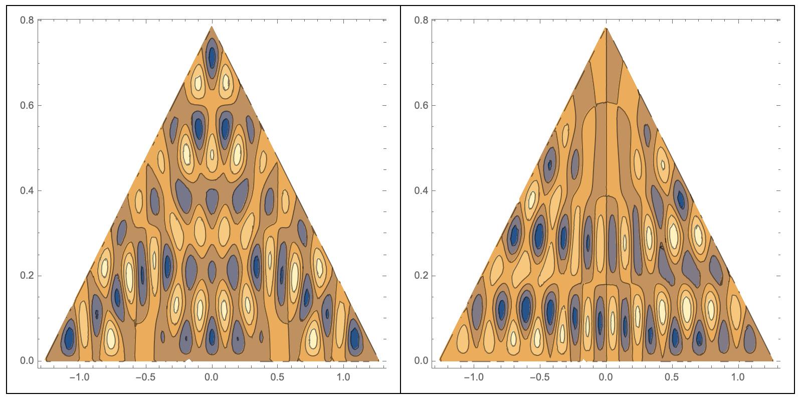
Figure 1: 92nd (left) and 95th (right) energy eigenstate of $\kappa$=24 (irrational isosceles) triangle. The left (right) panel shows a symmetric (an anti-symmetric) eigenstates with respect to the reflection axis.

3 Spectral statistics of triangular billiards

The degree of quantum chaos is controlled by short-range correlations and fluctuations in the energy eigenvalues. We want to compare these spectral statistics between the triangular billiards and chaotic, random matrix theories (RMTs), independently of the coarse-grained spectral density profile, which depends on non-universal characteristics like the overall area of the billiard. To do so, a standard procedure is to apply an “unfolding” process Haake2010 that uniformizes the spectral density so that the local statistics of different triangles can be compared. Given a density of states $\bar{\rho}(E)$ coarse-grained at some scale that is sufficiently larger than the typical energy gap, such a uniformisation can be realized by mapping

$$e_{j}=\bar{N}(\mathcal{E}_{j}),\quad\forall j,$$ (3)

where $\bar{N}(\mathcal{E}_{j})=\int_{-\infty}^{\mathcal{E}_{j}}dE\,\bar{\rho}(E)$ is the cumulative number of energy eigenvalues below $\mathcal{E}_{j}$. This procedure renders the spectrum $\left\{e_{j}\right\}$ macroscopically uniform while maintaining local fluctuations. However, unfolding effectively changes the Hamiltonian and will lead to different results for dynamical properties like the spread of the wavefunction. Hence, we follow an alternate procedure Bohigas:1983er ; Miltenburg1994 ; Lozej2022 ; yczkowski1992ClassicalAQ ; Cheon:levelpseudointegrable ; Bogomolny2021 ; Gorin_2001 ; barrierbilliards .

First, note that for triangle billiards, the cumulative number of energy levels below $\mathcal{E}$ asymptotes at large $\mathcal{E}$, after coarse-graining over a suitable scale larger than the typical gap, to the generalized Weyl formula Baltes1977 ; Miltenburg1994 ; Lozej2022

$$\bar{N}(\mathcal{E})=\frac{A\mathcal{E}-L\sqrt{\mathcal{E}}}{4\pi}+\frac{\pi}{24}\left(\frac{1}{\alpha}+\frac{1}{\beta}+\frac{1}{\gamma}-\frac{1}{\pi}\right),$$ (4)

with $\alpha$, $\beta$, $\gamma$ the three internal angles, $A$ the area of the triangle (set to $1$ in our analyses), and $L=A\frac{\sqrt{2}(\sin\alpha+\sin\beta+\sin\gamma)}{\sqrt{\sin\alpha\sin\beta\sin\gamma}}$ its perimeter. When $\mathcal{E}\gg(L/A)^{2}$, the cumulative count given by this “spectral staircase” formula is approximately linear in $\mathcal{E}$: $\bar{N}(\mathcal{E})\approx A\mathcal{E}/4\pi$. So, for sufficiently large energies, the coarse grained spectral density in any triangle is already uniform. Thus, in most analyses, we examine the truncated spectrum:

$$\left\{\mathcal{E}_{j}\right\}_{j=M}^{D_{0}-1}\quad\text{with}\quad\mathcal{E}_{M}\gg(L/A)^{2}\quad\text{and}\quad D\equiv D_{0}-M\,.$$ (5)

By doing so, we avoid the need for unfolding. In our numerical studies we examine the first $D_{0}=1000$ levels and find that for all the triangles we consider the Weyl formula linearizes for $j\gtrsim 50$ so that we can take $M=50$. Finally, we shift and rescale the truncated spectrum $\left\{\mathcal{E}_{j}\right\}_{j=M}^{D_{0}-1}$ so that the mean energy is $0$, while the spread of energies $E_{D}-E_{0}$ is $1$:

$$E_{j}=\frac{\mathcal{E}_{j+M}-\bar{\mathcal{E}}}{\mathcal{E}_{D_{0}-1}-\mathcal{E}_{M}},\quad\bar{\mathcal{E}}=\frac{1}{D}\sum_{j=M}^{D_{0}-1}\mathcal{E}_{j}.$$ (6)

This normalisation rescales the truncated spectrum to always occupy the same range so that we can consistently compare different triangles.

3.1 Level Spacing Ratio

The Level Spacing Ratio (LSR), which measures the ratio of the smaller and larger energy gaps around a level, differentiates spectral fluctuations for Poisson or random matrix statistics, without unfolding Atas:2013gvn . Thus we use the full spectrum up to the bound $D_{0}$ in (5) to examine LSRs for the triangle billiards, without the lower cutoff $M$. Denote by $p(s)$ the histogram of level spacings $\left\{s_{j}|j=1,2,\cdots,D-1\right\}$ where $s_{j}=\mathcal{E}_{j+1}-\mathcal{E}_{j}$ is the difference between consecutive energy levels $s_{j}=\mathcal{E}_{j+1}-\mathcal{E}_{j}$. This level spacing is reported to be Wigner-Dyson like the Gaussian Orthogonal RMT ensemble for non-integrable triangles; and, for pseudo-integrable triangles, tends to Wigner-Dyson (WD) for small spacings ($s\to 0$) and Poisson for large spacings ($s\to\infty$) Miltenburg1994 ; Lozej2022 ; yczkowski1992ClassicalAQ ; Cheon:levelpseudointegrable ; Bogomolny2021 ; Gorin_2001 ; barrierbilliards .

Define the average Level Spacing Ratio (LSR) as Oganesyan2007LSR

$$\bar{r}=\frac{1}{D_{0}-1}\sum_{n=1}^{D_{0}-1}\min\left(r_{j},\frac{1}{r_{j}}\right),\quad\text{ where }r_{j}=\frac{s_{j}}{s_{j+1}}.$$ (7)

The minimum means that we take the ratio of the smaller interval to the larger one so that $r_{j}\in[0,1]$. Since the LSR involves consecutive levels, it is independent of the local density of states and unfolding. Regular level spacing gives $\bar{r}=1$, and larger fluctuations produce a smaller average LSR. Poisson spectra have $\bar{r}_{\rm Poisson}\approx 0.3863$ and GOE spectra have $\bar{r}_{\rm GOE}\approx 0.5307$ Atas:2013gvn . For models with multiple degenerate energy levels, the ratio $r_{j}$ can be ill-defined for some $j$ because it is $0/0$. For such degenerate cases, we assign either the minimum value $0$ or the maximum value $1$ to all the ill-defined ratios, thus computing an upper and lower average LSR. Fig. 2 shows that the average LSR for our triangular billiards is organized in a hierarchy:

• Generic triangles (4 non-integrable and 4 pseudo-integrable), which lack symmetries or fine-tuned angles, have LSRs matching GOE statistics, suggesting long-term chaos.

• Right angled triangles (6 pseudo-integrable and 2 non-integrable) have LSRs slightly lower than the GOE.

• Isosceles triangles (6 pseudo-integrable and 2 non-integrable) have LSRs close to the Poisson value. However, their symmetric and antisymmetric sectors separately approach GOE statistics (Fig. 3), suggesting correlations within but not between sectors.

• The three integrable triangles have the lowest LSRs, suggesting even greater fluctuations in level spacing than expected from Poisson statistics. These triangles have substantial degeneracies in their spectra, and thus we report lower and upper average LSRs by replacing all ill-defined $0/0$ level spacing ratios by $0$ or $1$ as described above.

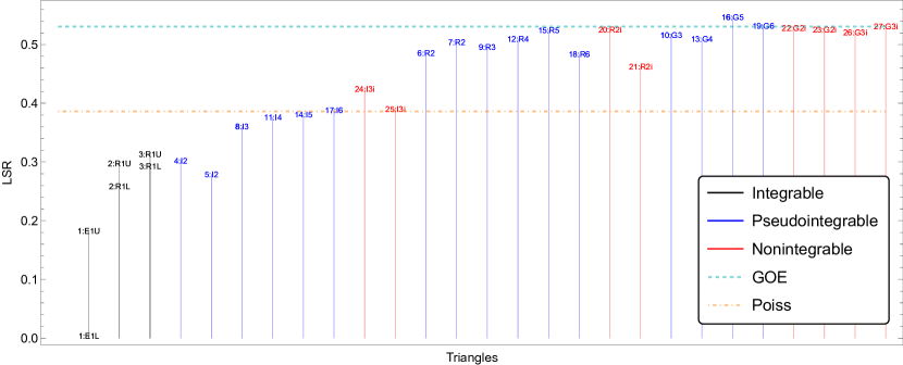
Figure 2: Level spacing ratio (LSR) for all 27 triangles. The data points are marked by labels of the form $\chi:Tg$. Here, $\kappa$ is the index of the triangle from Table 1, $T$ is the triangle type ($E$ = equilateral, $I$ = isosceles, $R$ = right, $G$ = general), and $g$ is the genus of the translation surface of the triangle. For irrational triangles which have infinite genus, we replace $g$ by $2i$ or $3i$ for triangles with 2 and 3 irrational angles, respectively. Sky blue dashed line = LSR for the Gaussian Orthogonal Ensemble (GOE). Orange dot-dashed line = LSR value for the Poisson distribution. Integrable and isosceles triangles approach the Poisson result. Generic and right triangles approach the GOE result. We report lower and upper average LSRs for the three integrable triangles by replacing all ill-defined $0/0$ level spacing ratios with either $0$ or $1$.

Figure 3: Level spacing ratio (LSR) for isosceles triangles. Data points marked using the same labels as Fig. 2. PI = pseudo-integrable and NI = non-integrable. $\kappa$:S and $\kappa$:A denote the symmetric and anti-symmetric sectors of the triangle indexed by $\kappa$. The total spectra of isosceles triangles have LSRs closer to Poisson, but their symmetric and anti-symmetric sectors have LSRs closer to GOE.

3.2 Spectral complexity

Next, we use the truncated spectra in (5) to calculate the spectral form factor (SFF) and the spectral complexity (SC) of our triangular billiards. The spectral form factor is

$$\operatorname{SFF}(t)=\sum_{jk}^{D}\exp(it(E_{j}-E_{k}))=\int dE_{1}\,dE_{2}\,\rho(E_{1})\,\rho(E_{2})\,e^{it(E_{1}-E_{2})}\,,$$ (8)

where $D$ is the dimension of the truncated Hilbert space and the spectral density is

$$\rho(E)=\sum_{j}\delta(E-E_{j})$$ (9)

with normalisation $\int dE\,\rho(E)=D$. If the spectrum is non-degenerate, the long time limit of the SFF converges to a plateau value $D$ Cotler:2016fpe , arising from the $j=k$ terms in (8). The spectral complexity is

$$C_{S}(t)=\sum^{D}_{j\neq k}\left[\frac{\sin(t(E_{j}-E_{k})/2)}{D(E_{j}-E_{k})/2}\right]^{2}=\int dE_{1}\,dE_{2}\,\rho(E)\,\rho(E_{2})\,\left[\frac{\sin(t(E_{1}-E_{2})/2)}{D(E_{1}-E_{2})/2}\right]^{2},$$ (10)

For systems with non-degenerate spectra, since $\sin^{2}(t(E_{j}-E_{k})/2)\leq 1$ in (10), the SC is bounded above by $\left(\frac{2}{\Delta E_{\min}}\right)^{2}$, with $\Delta E_{\min}$ the minimal level spacing. Since we have rescaled the spectrum to have a width of 1, the minimal level spacing $\Delta E_{\min}$ scales as $1/D$. For systems with degenerate spectra, taking the limit $E_{j}-E_{k}\to 0$ in (10) reveals that SC will grow as $\frac{d}{D^{2}}t^{2}$ at late times, with $d=\sum_{j\neq k}\delta_{E_{j}E_{k}}$. Provided the SFF approaches a late time plateau of $D$, as it does for non-degenerate spectra, the SFF and SC are simply related by Iliesiu:2021ari ; Erdmenger:2023wjg

$$C_{S}(t)=\frac{2}{D^{2}}\int_{0}^{t}dt^{\prime}\int_{0}^{t^{\prime}}dt^{\prime\prime}(\operatorname{SFF}(t^{\prime\prime})-D).$$ (11)

First we work out the result for spectra with Poisson and GOE statistics. As discussed in (5) we work in an energy for the triangle billiards in which the cumulative number of states grows linearly with energy, so that the coarse-grained spectral density is constant

$$\bar{\rho}(E)=d\bar{N}/dE=D.$$ (12)

It would be useful to know how the SFF and SC behave for theories with the coarse-grained level density (12) and either no spectral correlations, as expected for an integrable theory, or GOE correlations, as expected for a maximally chaotic theory. We can study this by taking the expectation value of (8) and (10) over Poisson or Gaussian Orthogonal ensembles. Doing so amounts to replacing the $\rho(E_{1})\rho(E_{2})$ factors by ensemble average, which gives the density-density correlation function.

If the theory is integrable, we expect that there are no spectral correlations so that the density-density correlation function at large $D$ is

$$\left\langle\rho(E_{1})\rho(E_{2})\right\rangle=\bar{\rho}(E)\delta(s)+\left(1-\frac{1}{D}\right)\bar{\rho}(E_{1})\bar{\rho}(E_{2})\,,$$ (13)

where $E=(E_{1}+E_{2})/2,\ s=E_{1}-E_{2}$ Haake2010 . Inserting this into (8), along with the coarse-grained spectral density (12), we obtain the SFF

$$\operatorname{SFF}(t)=(D-1)D\operatorname{sinc}^{2}\frac{t}{2}+D\approx\begin{cases}4D^{2}\operatorname{sinc}^{2}{\frac{t}{2}}\,,&t\ll\sqrt{D}\\ D\,,&\sqrt{D}\ll t\end{cases}\,,$$ (14)

where $\operatorname{sinc}t=\frac{\sin t}{t}$. This SFF slopes quadratically down a maximum value of $D^{2}$ until $t\sim\sqrt{D}$ when it crosses over to a plateau value of $D$. For Poisson-distributed spectra with finite $D$, exact degeneracies are measure 0, so we can apply (11) to compute the SC. Since the SFF is always greater than or equal to its plateau value $D$, the integrand of (11) is always non-negative, which implies eternal growth of the SC at late times. Indeed by performing the double integral over time in (11) we obtain the spectral complexity

$$C_{S}(t)=4\left(1-\frac{1}{D}\right)(\operatorname{Ci}(t)+t\operatorname{Si}(t)-\log(t)+\cos(t)-\gamma-1)\approx\begin{cases}t^{2},&t\ll 1\\ 2\pi t,&1\ll t\,,\end{cases}$$ (15)

with $\operatorname{Ci}(t)=-\int_{t}^{\infty}dz\frac{\cos z}{z},\ \operatorname{Si}(t)=\int_{0}^{t}dz\frac{\sin z}{z}$, and Euler’s constant $\gamma$. Thus, for Poisson distributed spectra, the SC grows linearly at late times.

For random matrix theories drawn from the GOE, the spectrum is correlated as:

$$\left\langle\rho(E_{1})\rho(E_{2})\right\rangle=\bar{\rho}(E)\delta(s)+\bar{\rho}(E_{1})\bar{\rho}(E_{2})(1-\hat{k}(\pi Ds)),$$ (16)

where

$$\hat{k}(x)=\operatorname{sinc}^{2}x+\frac{1}{x}(\operatorname{Si}(x)-\frac{\pi}{2}\mathrm{sgn}x)(\operatorname{sinc}x-\cos x)$$ (17)

is related to the well-known sine kernel in the GOE Haake2010 ; Cotler:2016fpe ; Liu:2018hlr . Inserting the two-point function into (8), along with the spectral density (12), we can approximate the integral $\iint_{0}^{1}dE_{1}dE_{2}\hat{k}(\pi Ds)e^{its}\approx\int_{0}^{1}dE\int_{-\infty}^{\infty}ds\hat{k}(\pi Ds)e^{its}$ at large $D$, because the kernel $\hat{k}(\pi Ds)$ is localized at $s=0$ with a width $1/D$ Liu:2018hlr . Then the SFF is

$$\operatorname{SFF}(t)= ~{}D^{2}\operatorname{sinc}^{2}\frac{t}{2}+D+\begin{cases}\frac{t}{\pi}-D-\frac{t}{2\pi}\log\left(1+\frac{t}{\pi D}\right),&t<2\pi D\\ D-\frac{t}{\pi}\coth^{-1}\frac{t}{\pi D},&t\geq 2\pi D\\ \end{cases}$$ (18)

$$\approx ~{}\begin{cases}4D^{2}\operatorname{sinc}^{2}\frac{t}{2}\,,&t\ll D^{2/3}\\ \frac{t}{\pi}\,,&D^{2/3}\ll t\ll D\\ D\,,&D\ll t\end{cases}.$$ (19)

It exhibits a slope down to a minimum at a “dip time” $t\sim D^{2/3}$, and then ramps linearly upward up to a late time plateau of magnitude $D$. Since the SFF is smaller than its plateau value $D$ during the ramp, (11) implies that the spectral complexity should grow more slowly after the dip time. Inserting the two-point function into (10) and again using the localisation of $\hat{k}(\pi Ds)$, we obtain the spectral complexity

$$C_{S}(t)= ~{}4(\operatorname{Ci}(t)+t\operatorname{Si}(t)-\log(t)+\cos(t)-\gamma-1)+DC_{1}\left(\frac{t}{\pi D}\right)$$ (20)

$$\to ~{}\begin{cases}t^{2},&t\ll 1\\ 2\pi t,&1\ll t\ll D\\ \frac{2}{3}\pi^{2}D\log\left(\frac{t}{\pi D}\right),&D\ll t\end{cases}$$ (21)

where

$$C_{1}(u)=~{}\frac{\pi^{2}}{3}\begin{cases}{u\left(\frac{17}{12}u^{2}-4u-1\right)+(1-\frac{u}{2})(u+1)^{2}\log(u+1)},&u<2\\ {\log\left(u^{2}-1\right)-\left(u^{2}-3\right)u\coth^{-1}u+(u-6)u+\frac{4}{3}},&u>2\\ \end{cases}.$$ (22)

Thus, at late times, spectral complexity for the GOE exhibits logarithmic growth.

The above analytical calculations show that, for the same spectral density, uncorrelated spectra lead to faster late time growth of SC than for GOE-correlated spectrum (Fig. 4.) Note that these expressions are valid in the leading large $D$ limit for rescaled spectra with a bounded range. In this limit, the minimum gap $\Delta E_{\min}$ goes to zero, so the SC bound of $\left(\frac{2}{\Delta E_{\min}}\right)^{2}$ becomes trivial. Fig. 4 shows that the late time growth of spectral complexity for our triangular billiards shows a variety of behaviours:

• Generic triangles (4 non-integrable and 4 pseudo-integrable), which lack symmetries or fine-tuned angles, show slow late time growth like the GOE.

• Right angled triangles (6 pseudo-integrable and 2 non-integrable) also show slow late growth of spectral complexity but, on average, reach slightly higher late time values.

• Isosceles triangles (6 pseudo-integrable and 2 non-integrable) closely match Poisson late time linear growth of spectral complexity. However, Fig. 5, shows that the antisymmetric sectors of all these theories show slow late time growth comparable to the GOE, while the symmetric sectors typically show a longer period of linear growth before slowing down, and even in some cases decreasing markedly towards the GOE. Both symmetric and antisymmetric sectors also show large late time oscillations of spectral complexity. It would be interesting to understand why the SC of these two sectors behaves so differently, although their LSRs are similar (Fig. 3).

• The three integrable triangles have substantial spectral degeneracies which lead to late time quadratic SC growth as expected from the discussion below (10).

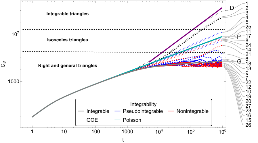
Figure 4: Spectral complexity of all the 27 billiards. The numbers on the right show the $\kappa$ index of the triangles as defined in Table 1. The labels P, G and D denote our analytical prediction of the spectral complexity growth for models with Poisson (proportional to $t$ at late times), GOE (logarithmic in $t$ at late times) and degenerate spectra (proportional to $t^{2}$ at late times) with the same degeneracy as that in the equilateral triangle $1$. Dotted lines are for isosceles triangles, dashed lines are for right triangles, and solid lines (except the three denoted P, G and D) are for general triangles. The integrable triangles with degenerate spectra show quadratic late time growth, while the non-integrable triangles match logarithmic late time growth except for the GOE. The isosceles triangles show linear late time growth similar to that expected for a Poisson spectrum.

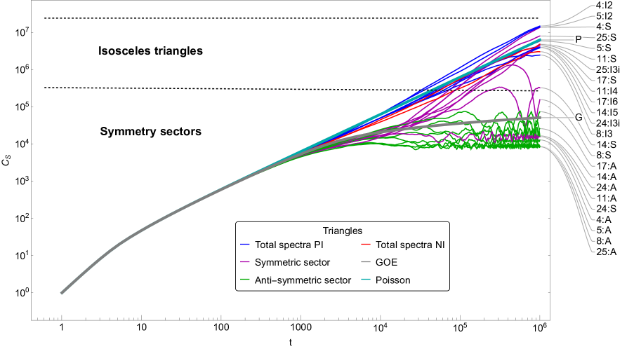
Figure 5: Spectral complexity for isosceles triangles. Labels match those in Fig. 3. The labels P and G denote the Poissonian and GOE spectral complexity, respectively. The isosceles triangles show linear growth at late times, but their anti-symmetric sectors more closely match the GOE behaviour, while their symmetric sectors also deviate dramatically from linear growth. Both symmetry sectors show large late time oscillations.

4 Spread complexity in triangular billiards

Next, we will show how the spread complexity and other Krylov space probes, such as the variance of the Lanczos coefficients and the inverse participation ratio of energy eigenstates in the Krylov space, distinguish integrable and chaotic dynamics in triangular billiards Edwards_1972 ; Misguich_2016 ; Rabinovici:2021qqt ; Bhattacharjee:2024yxj . As the Hilbert space of these systems is infinite-dimensional, we first truncate it for operational purposes to the $D=1000$ lowest energy eigenstates, over which the initial state is uniformly spread

$$|\psi(0)\rangle=\frac{1}{\sqrt{D}}\sum_{j=0}^{D-1}|E_{j}\rangle\,.$$ (23)

The state undergoes time evolution under the Hamiltonian: $|\psi(t)\rangle=e^{-iHt}|\psi(0)\rangle$. We calculate the Lanczos coefficients $\{a_{n},b_{n}\}$ and build the orthogonal Krylov basis $\{|O_{n}\rangle\}_{n=0}^{D-1}$ following Viswanath1994 ; Lanczos:1950zz :

$$\left|O_{0}\right\rangle =\left|\psi(0)\right\rangle,\quad b_{0}=0,$$

$$b_{n}\left|O_{n}\right\rangle =(H-a_{n-1})\left|O_{n-1}\right\rangle-b_{n-1}\left|O_{n-2}\right\rangle,\quad 1\leq n\leq K-1,$$ (24)

$$a_{n} =\left\langle O_{n}\right|H\left|O_{n}\right\rangle,\quad\left\langle O_{n}|O_{n}\right\rangle=1.$$

The algorithm terminates at some $n=K$ when $b_{K}=0$ giving a Krylov space of dimension $K\leq D$ (examples in Fig. 6). This procedure is equivalent to tridiagonalizing the Hamiltonian:

$$T_{mn}=\left\langle O_{m}\right|H\left|O_{n}\right\rangle=\begin{pmatrix}a_{0}&b_{1}&0&\cdots&0\\ b_{1}&a_{1}&b_{2}&\cdots&0\\ 0&b_{2}&a_{2}&\cdots&0\\ \vdots&\vdots&\vdots&\ddots&b_{K-1}\\ 0&0&0&b_{K-1}&a_{K-1}\end{pmatrix}.$$ (25)

To quantify how the wavefunction spreads, we measure the support of the time-evolved state has on Krylov basis vectors:

$$|\phi_{n}(t)|^{2}=|\langle O_{n}|\psi(t)\rangle|^{2}\,.$$ (26)

We can characterize this distribution in terms of its moments

$$C^{(\alpha)}_{K}(t)=\sum_{n=0}^{N-1}n^{\alpha}|\phi_{n}(t)|^{2}.$$ (27)

The $\alpha=1$ moment is called the spread complexity Balasubramanian:2022tpr , but the higher moments are useful to consider because they amplify features of the dynamics associated to chaos Balasubramanian:2022tpr ; Erdmenger:2023wjg .

4.1 Variance of the Lanczos coefficients

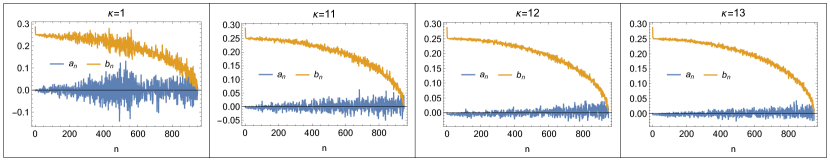
Figure 6: Left to right: Lanczos coefficients $a_{n}$ and $b_{n}$ for $\kappa$=1 (integrable, equilateral), $\kappa$=11 (pseudo-integrable, isosceles), $\kappa$=12 (pseudo-integrable, right), $\kappa$=13 (pseudo-integrable, general) triangles. The variance is the highest for the integrable triangle.

It has been observed that higher classical Lyapunov exponents are associated with lower variance in the Lanczos coefficients Hashimoto:2023swv . But in our case, the classical Lyapunov exponents vanish, as they do for all polygonal billiards Jain_2017 . On the other hand, the authors of Hashimoto:2023swv ; Balasubramanian:2023kwd proposed that the variance of the Lanczos coefficients provides a signature discriminating between integrability and chaos. We therefore calculate the standard deviations

$$\sigma(a_{n})=\sqrt{\sum_{n}x_{n}^{2}-\left(\sum_{n}x_{n}\right)^{2}},\quad x_{n}=a_{n+1}-a_{n}$$ (28)

$$\sigma(2b_{n})=\sqrt{\sum_{n}y_{n}^{2}-\left(\sum_{n}y_{n}\right)^{2}},\quad y_{n}=2b_{n+1}-2b_{n}.$$ (29)

We are studying the standard deviations of $\left\{a_{n},2b_{n}\right\}$ because, for a random state initial state and evolution with a random matrix Hamiltons, their variances $a_{n}$ and $2b_{n}$ are equal Balasubramanian:2022dnj ; Balasubramanian:2023kwd . Note that these definitions of variance differ from those used in Rabinovici:2021qqt ; Hashimoto:2023swv .

Fig. 7 shows a clear trend. Integrable triangles have by far the largest variance in their Lanczos coefficients, followed by isosceles triangles. Right triangles come next, with Lanczos variance generally larger than those of the generic pseudo-integrable triangles, which are in turn larger than those of non-integrable triangles (Fig. 7 inset). Interestingly, the Lanzos variances are anti-correlated with the Level Spacing Ratio (LSR): the higher the LSR, the lower the Lanczos variance (Fig. 7). Low LSRs suggest high level repulsion and spectral correlation, perhaps leading to less statistical independence, and hence variance, between the Lanczos coefficients.

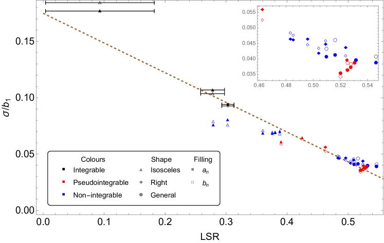
Figure 7: Standard deviations normalized by $b_{1}$ ($\sigma/b_{1}$) of $\left\{a_{n},2b_{n}\right\}$ vs. level spacing ratio for all 27 triangle billiards. For the integrable triangles, the error bars represent the range between the upper and lower average LSRs computed by replacing all ill-defined $0/0$ level spacing ratios by either $0$ or $1$. Small values of level spacing ratio correlate to high values of the standard deviation of the Lanczos coefficients. The dashed brown line is a linear fit of the data points: using the average of the upper and lower LSRs for integrable triangles, we find a slope of $-0.262$ and a positive y-axis intercept of 0.174. Inset: Focus on non-isosceles, pseudo-integrable and non-integrable triangles.

4.2 Localisation of energy eigenstates in Krylov space

Next, we consider the overlap $\left|\langle O_{n}|E_{j}\rangle\right|$ between the energy basis and the Krylov basis (Fig. 8). The overlap $\left|\langle O_{n}|E_{j}\rangle\right|$ is approximately zero for energies $\left|E_{j}\right|>2b_{n}$ Erdmenger:2023wjg . This concentration can be understood by noting that, as shown in Eq. 39 of Balasubramanian:2023kwd ,

$$\sum_{E^{\prime}\in[E,E+dE]}|\langle K_{m}|E^{\prime}\rangle|^{2}\approx\frac{\Theta(4b_{m}^{2}-(E-a_{m})^{2})}{\pi\sqrt{4b_{m}^{2}-(E-a_{m})^{2}}}\,dE$$ (30)

where $dE$ is a small interval of energies. Since $b_{m}$ is on average a decreasing function of $m$ and $a_{m}$ is zero on average (Fig. 6), $\langle O_{n}|E_{j}\rangle$ tends to vanish for $\left|E_{j}\right|>2b_{n}$. Thus, low energy and high energy eigenstates tend to be located in the Krylov basis with small $n$ (Fig. 8). Note that this is a general phenomenon that depends on the coarse-grained spectral density and is independent of integrability or chaos in the dynamics.

For the integrable triangles, the overlap $\left|\langle O_{n}|E_{j}\rangle\right|$ for a given $j$ concentrates at some $n$ although this is not readily visible in Fig. 8 because nearest neighbour energy eigenstates can localise onto different Krylov basis vectors. The authors of Dymarsky:2019quantum ; Rabinovici:2021qqt ; Bhattacharjee:2024yxj explain this sort of phenomenon as a form of Anderson localisation in the Krylov basis, that can be traced to disorder in the Lanczos coefficients of integrable triangles (see related comments in Balasubramanian:2023kwd ). To quantify this localisation, we study the Inverse Participation Ratio (IPR) of energy eigenstates in the Krylov basis:

$$\text{IPR}_{j}=\sum_{n=1}^{K}|\langle O_{n}|E_{j}\rangle|^{4}.$$ (31)

IPR_j quantifies how localized an energy eigenstate is in the Krylov basis. If an eigenstate is completely localized, $|E_{j}\rangle=|O_{n}\rangle$, so that IPR${}_{j}=1$. Conversely, if a state is entirely delocalized, $|E_{n}\rangle=\frac{1}{\sqrt{K}}\sum_{j=1}^{K}|O_{j}\rangle$, and IPR${}_{j}=1/K$. The higher the IPR, the more pronounced the localisation. The IPR for the entire system is defined by summing over all the energy eigenstates:

$$\text{IPR}=\sum_{j=1}^{D}\text{IPR}_{j}=\sum_{j=1}^{D}\sum_{n=1}^{K}|\langle O_{n}|E_{j}\rangle|^{4}.$$ (32)

Fig. 9 shows a clear hierarchy. The integrable triangles show the greatest localisation of energy eigenstates, followed by isosceles triangles, right triangles and generic pseudo-integrable and non-integrable triangles.

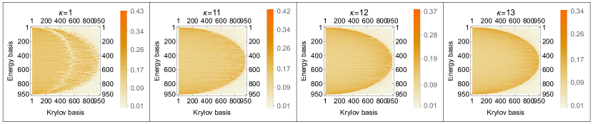
Figure 8: Left to right: Overlap matrix of the energy eigenstates with the Krylov basis, $|\langle E_{j}|O_{n}\rangle|$ for $\kappa$=1 (integrable, equilateral), $\kappa$=11 (pseudo-integrable, isosceles), $\kappa$=12 (pseudo-integrable, right), $\kappa$=13 (pseudo-integrable, general) triangles. The localisation of energy basis on the Krylov basis vectors is the highest for the integrable triangles (see text), but this concentration is not readily visible because nearby energy eigenstates can localize onto different Krylov states.

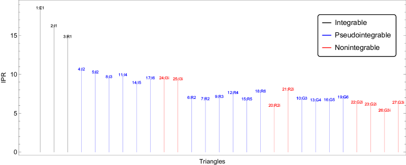
Figure 9: Inverse participation ratio for all 27 triangles. Data points are marked by labels of the form $\chi:Tg$. Here, $\kappa$ is the index of the triangle from Table 1, $T$ is the triangle type ($E$ = equilateral, $I$ = isosceles, $R$ = right, $G$ = general), and $g$ is the genus of the translation surface of the triangle. For irrational triangles which have infinite genus, we replace $g$ by $2i$ or $3i$ for triangles with 2 and 3 irrational angles, respectively. IPR is highest for integrable triangles, followed by isosceles, right and generic triangles.

4.3 Spread complexity

Finally we compute spread complexity for our triangular billiards (Figs. 10(a), 10(b)). There is a striking difference between the integrable triangles and all the rest: the spread complexity rises to a plateau, exhibits some oscillations and then drops dramatically to zero, indicating the start of a recurrence. This is as expected: in quantum systems with finite dimension $K$, Poincaré recurrences are expected to happen at timescale $e^{K}$ for non-integrable systems and timescale $K$ for integrable systems PhysRev.107.337 . Indeed, the spread complexity of the integrable triangle billiards drops to zero periodically, suggesting that the system has returned to its initial state at these Poincaré quantum recurrence times PhysRev.107.337 . The recurrences arise from commensurability of the integrable triangle spectra Hashimoto:2023swv ; Doncheski_2002 ; Jung1980 ; Damle2010 ; RICHENS1981495 , and the lower plateau value occurs because of the higher variance of the Lanczos coefficients Rabinovici:2021qqt . By contrast, the general pseudo-integrable and non-integrable triangles all show spread complexity characteristic of chaotic dynamics, namely an initial rise to a peak, followed by a slope downward to a plateau Balasubramanian:2022tpr ; Balasubramanian:2023kwd .

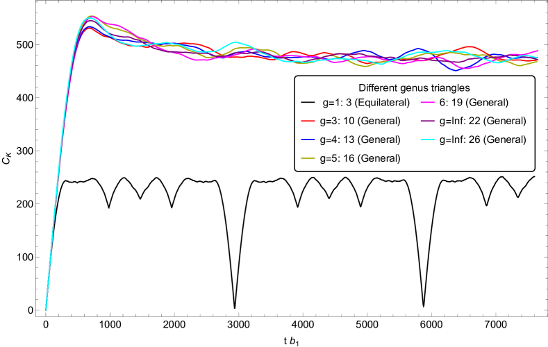
(a) Spread complexity ($\alpha=1$ in Eq.(27)) for different genus of triangular billiards.

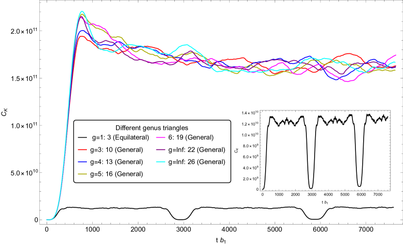
(b) $4$th moment of spread complexity ($\alpha=4$ in Eq.(27)) for different genus of triangular billiards.

Figure 10: Spread complexity and its fourth moment for triangles corresponding to different genera, i.e., $\kappa$=1 (genus one equilateral), $\kappa$=10 (genus three general), $\kappa$=13 (genus four general), $\kappa$=16 (genus five general), and $\kappa$=19 (genus six general) triangle. The integrable triangle corresponding to genus one has oscillatory complexity, whereas the pseudo-integrable and non-integrable general triangles show the characteristic behaviour or growth-peak-decay and saturation.

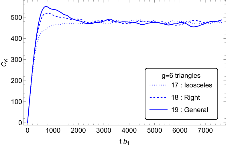
(a) Spread complexity ($\alpha=1$ in Eq.(27)) for different types of triangular billiards

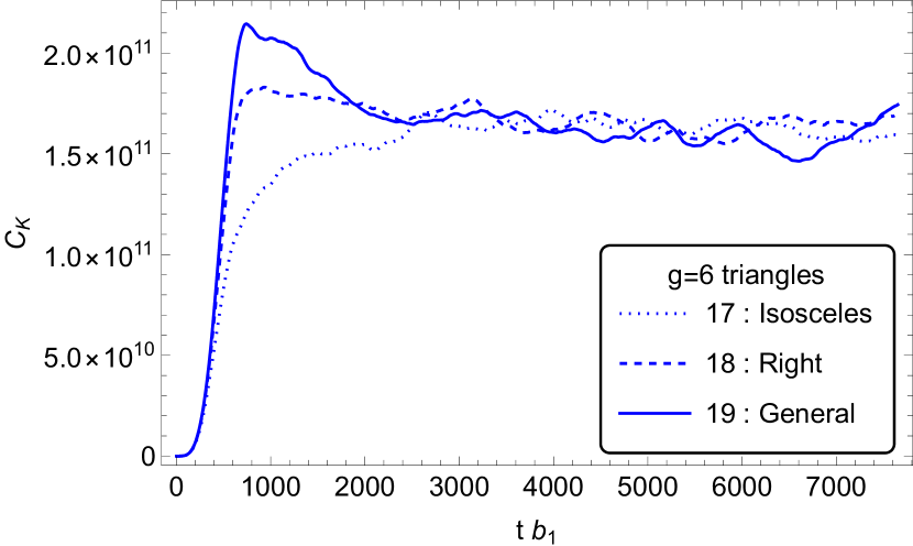
(b) $4$th moment of spread complexity ($\alpha=4$ in Eq.(27)) for different types of triangular billiards

Figure 11: Spread complexity and its fourth moment for triangles with genus six translation surfaces: $\kappa$=17 (isosceles), $\kappa$=18 (right) and $\kappa$=19 (general). The height of the complexity peak is reduced by the presence of symmetries. This difference becomes more pronounced for the higher moments of complexity.

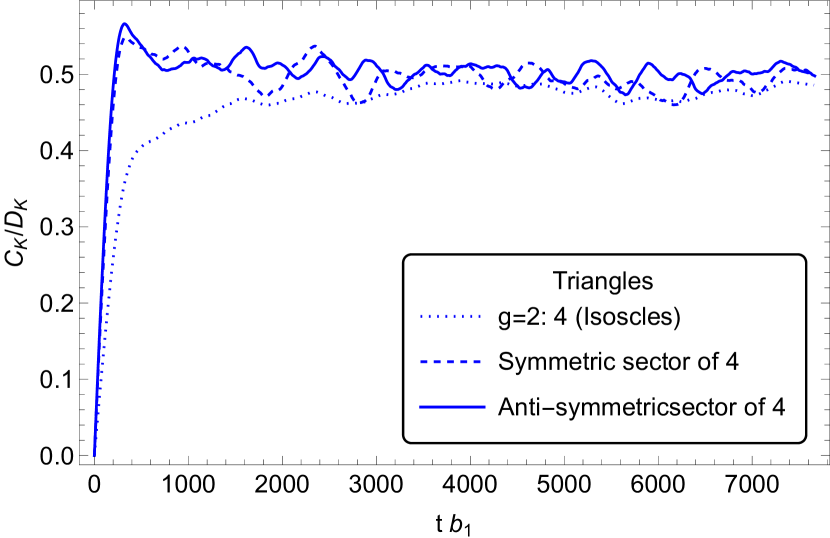
(a) Spread complexity ($\alpha=1$ in Eq.(27)) for the symmetric and anti-symmetric sectors of isosceles triangular billiard

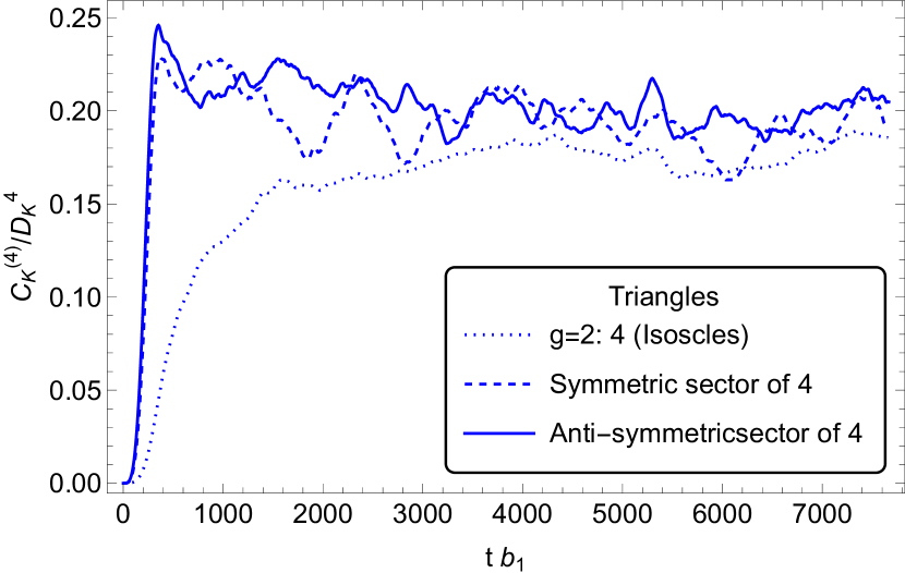
(b) $4$th moment of Spread complexity ($\alpha=4$ in Eq.(27)) for the symmetric and anti-symmetric sectors of isosceles triangular billiard

Figure 12: Spread complexity and its fourth moment the symmetric and anti-symmetric sectors of isosceles triangular billiards with genus two translation surfaces and $\kappa$=4. The individual symmetry sectors display a complexity peak characteristic of chaotic systems, while the complete dynamics does not show this feature.

Symmetry reduces or eliminates the characteristic feature of chaos – the spread complexity peak Balasubramanian:2022tpr ; Hashimoto:2023swv ; Balasubramanian:2023kwd : this peak is absent for isosceles triangles and reduced for right triangles, both of which have special symmetries (Fig. 11). The even and odd symmetry sectors of the the isosceles triangles separately show spread complexity complexity growth resembling chaotic theories (rise to a peak, followed by slope down to a plateau), but the complexity growth in the combined dynamics lacks these features (Fig. 12).

5 Summary and outlook

In this paper, we surveyed the quantum dynamics of twenty-seven triangular billiards, which can display a variety of dynamics – integrable, pseudointegrable and non-integrable – controlled by the internal angles of the triangles. We characterized these theories spectrally in terms of their level spacing ratios and spectral complexity and then in terms of the variance in their Lanczos coefficients, localisation of energy eigenstates in the Krylov basis, and dynamical growth of spread complexity. We find that:

• Integrable triangles have the lowest level spacing ratios (LSRs) and hence the highest level spacing fluctuations. Degeneracies in their spectrum lead to quadratic late time spectral complexity growth, even faster than the linear growth expected for Poisson-distributed spectra. Their Lanczos coefficients show the largest variances, and partly as a consequence, their energy eigenstates are strongly localized in the Krylov basis. Finally, spread complexity for the integrable billiards does not show the complexity peak characteristic of chaos, and also displays marked Poincare recurrences.

• Isosceles triangles from either the pseudo-integrable or the non-nonintegrable classes display LSRs and linearly growing spread complexity growth close to that expected for theories with Poisson spectra. Their Lanczos spectra have variances that are smaller than the integrable triangles, but substantially larger than triangles that lack symmetries. Likewise, their energy eigenstates are less localized in the Krylov chain than the integrable triangles but more so than generic triangles. The spread complexity for isosceles triangles does not show the marked recurrences seen for integrable triangles but lacks the peak that is characteristic of chaos.

• The symmetric and anti-symmetric sectors of isosceles triangles, from either the pseudo-integrable or the non-nonintegrable classes, separately display LSRs close to the Gaussian Orthogonal Ensemble (GOE) value, but the spectral complexity shows substantial oscillations before approaching the GOE result, with marked differences between the symmetry sectors. Similarly, the spread complexity of the two symmetry sectors separately shows a rise to a peak followed by a slope down to a plateau, even though the combined system does not display this characteristic of chaos.

• Right triangles of the pseudo-integrable and non-integrable classes have spectral features that are harder to discriminate from the generic triangle, but the LSRs are, on average, a little lower than the expected GOE value, although significantly higher than the Poisson value. Consistently, on average, their spectral complexity growth is slightly faster, their Lanczos variance slightly higher, and their energy eigenstate localisation slightly greater than for generic triangles. The spread complexity growth shows characteristic signs of chaos and does not differ from that of generic triangles at our numerical resolution.

• Generic pseudo-integrable triangles have level spacing ratios and spectral complexity growth close to the predicted behaviour of random matrix theories drawn from the GOE. The variances of the Lanczos coefficients are low, but slightly higher than for generic non-integrable triangles. Likewise, their energy eigenstates are less localized than most of the kinds of triangles we studied, but perhaps a bit more so than the general non-integrable triangles (although this requires a more precise numerical study). Finally, their spread complexity growth closely matches the expectation for chaotic theories.

• Generic non-integrable triangles have level spacing ratios and spectral complexity growth that match the expectation for GOE theories. They have the lowest Lanczos coefficient variance, energy eigenstates that are the most delocalized in the Krylov basis, and spread complexity growth that is precisely as expected for chaotic theories.

It would be useful to conduct higher precision numerical analyses to better discriminate the pseudo-integrable and non-integrable theories. Notably, all the triangle billiards have vanishing classical Lyapunov exponent, and chaotic behaviour arises from the pattern of splitting of beams of trajectories at the corners or, equivalently, the topology of the translation surface. In terms of the latter, there is a dramatic difference between the topology of the finite genus pseudo-integrable and infinite genus non-integrable translation surfaces. Where does this difference appear in the quantum dynamics? Possibly a path integral perspective would help, by making explicit trajectories that traverse different handles of the translation surface, and the corresponding contributions to quantum time evolution. It is also possible that these sorts of effects manifest themselves in patterns of “scarring”, i.e., localisation of quantum wavefunctions around clusters of classical paths Heller:stadiumscar ; Bogomolny2021 .

More broadly, the methods for quantifying chaos described above should be extended to quantum field theories, especially theories dual to gravity, in which simple initial states can rapidly form complex final states with macroscopic descriptions as black holes. It might be helpful to start with simplified models such as the chiral CFTs that are dual to the near-horizon physics of extremal black holes of string theory Balasubramanian:2003kq ; Balasubramanian:2009bg , or with an appropriately simplified sector of the interacting matrix model dual to M theory Banks:1996vh ; Balasubramanian:1997kd ; Polchinski:1999br . Alternatively, a further step in this direction is to extend the methods discussed here to spin-chain models motivated by holography Basteiro:2022zur ; Basteiro:2022xvu ; Basteiro:2024cuh .

References

- (1) O. Bohigas, M.J. Giannoni and C. Schmit, Characterization of chaotic quantum spectra and universality of level fluctuation laws, Phys. Rev. Lett. 52 (1984) 1.
- (2) M.V. Berry, Semiclassical theory of spectral rigidity, Proceedings of the Royal Society of London. A. Mathematical and Physical Sciences 400 (1985) 229.
- (3) S. Muller, S. Heusler, P. Braun, F. Haake and A. Altland, Semiclassical foundation of universality in quantum chaos, Phys. Rev. Lett. 93 (2004) 014103 [nlin/0401021].
- (4) F. Haake, Quantum Signatures of Chaos, Springer Berlin Heidelberg (2010), 10.1007/978-3-642-05428-0.
- (5) F.J. Dyson, A class of matrix ensembles, Journal of Mathematical Physics 13 (1972) 90–97.
- (6) T. Guhr, A. Muller-Groeling and H.A. Weidenmuller, Random matrix theories in quantum physics: Common concepts, Phys. Rept. 299 (1998) 189 [cond-mat/9707301].
- (7) C. Lozej, G. Casati and T. Prosen, Quantum chaos in triangular billiards, Physical Review Research 4 (2022) .
- (8) J. Maldacena, S.H. Shenker and D. Stanford, A bound on chaos, Journal of High Energy Physics 2016 (2016) .
- (9) I. García-Mata, R. Jalabert and D. Wisniacki, Out-of-time-order correlations and quantum chaos, Scholarpedia 18 (2023) 55237.
- (10) V. Balasubramanian, P. Caputa, J.M. Magan and Q. Wu, Quantum chaos and the complexity of spread of states, Phys. Rev. D 106 (2022) 046007 [2202.06957].
- (11) P. Richens and M. Berry, Pseudointegrable systems in classical and quantum mechanics, Physica D: Nonlinear Phenomena 2 (1981) 495.
- (12) S.R. Jain and R. Samajdar, Nodal portraits of quantum billiards: Domains, lines, and statistics, Reviews of Modern Physics 89 (2017) .
- (13) R. Frigg, J. Berkovitz and F. Kronz, The Ergodic Hierarchy, in The Stanford Encyclopedia of Philosophy, E.N. Zalta, ed., Metaphysics Research Lab, Stanford University (2020).
- (14) E. Ott, Chaos in Dynamical Systems, Cambridge University Press (Aug., 2002), 10.1017/cbo9780511803260.
- (15) A. Vikram and V. Galitski, Dynamical quantum ergodicity from energy level statistics, Phys. Rev. Res. 5 (2023) 033126.
- (16) N. Jha and S.R. Jain, Quantum mechanics of a rotating billiard, in Proceedings of the 12th Asia Pacific Physics Conference (APPC12), Journal of the Physical Society of Japan, Mar., 2014, DOI.
- (17) S.R. Jain, Proliferation law of periodic orbits of an integrable billiard as obtained from the eigenvalue spectrum, Phys. Rev. E 50 (1994) 2355.
- (18) R. Samajdar and S.R. Jain, A nodal domain theorem for integrable billiards in two dimensions, Annals of Physics 351 (2014) 1–12.
- (19) R. Samajdar and S.R. Jain, Exact eigenfunction amplitude distributions of integrable quantum billiards, Journal of Mathematical Physics 59 (2018) .
- (20) H.D. Parab and S.R. Jain, Non-universal spectral rigidity of quantum pseudo-integrable billiards, Journal of Physics A: Mathematical and General 29 (1996) 3903.
- (21) D. Biswas and S.R. Jain, Quantum description of a pseudointegrable system: The /3-rhombus billiard, Phys. Rev. A 42 (1990) 3170.
- (22) S. Moudgalya, S. Chandra and S.R. Jain, A finite-time exponent for random ehrenfest gas, Annals of Physics 361 (2015) 82.
- (23) R.B.d. Carmo and T.A. Lima, Mixing property of symmetrical polygonal billiards, Phys. Rev. E 109 (2024) 014224.
- (24) N. Chernov and S. Troubetzkoy, Ergodicity of billiards in polygons with pockets, Nonlinearity 11 (1998) 1095.
- (25) C. Lozej and E. Bogomolny, Intermediate spectral statistics of rational triangular quantum billiards, 2405.05783.
- (26) L.V. Iliesiu, M. Mezei and G. Sárosi, The volume of the black hole interior at late times, JHEP 07 (2022) 073 [2107.06286].
- (27) H.A. Camargo, V. Jahnke, H.-S. Jeong, K.-Y. Kim and M. Nishida, Spectral and Krylov complexity in billiard systems, Phys. Rev. D 109 (2024) 046017 [2306.11632].
- (28) Y. Sekino and L. Susskind, Fast scramblers, JHEP 10 (2008) 065 [0808.2096].
- (29) D.A. Roberts, D. Stanford and L. Susskind, Localized shocks, JHEP 03 (2015) 051 [1409.8180].
- (30) D.A. Roberts, D. Stanford and A. Streicher, Operator growth in the syk model, JHEP 06 (2018) 122 [1802.02633].
- (31) D.E. Parker, X. Cao, A. Avdoshkin, T. Scaffidi and E. Altman, A universal operator growth hypothesis, Phys. Rev. X 9 (2019) 041017 [1812.08657].
- (32) A. Kar, L. Lamprou, M. Rozali and J. Sully, Random matrix theory for complexity growth and black hole interiors, JHEP 01 (2022) 016 [2106.02046].
- (33) P. Caputa, J.M. Magan and D. Patramanis, Geometry of krylov complexity, Phys. Rev. Res. 4 (2022) 013041 [2109.03824].
- (34) A. Dymarsky and M. Smolkin, Krylov complexity in conformal field theory, Phys. Rev. D 104 (2021) L081702 [2104.09514].
- (35) J. Barbón, E. Rabinovici, R. Shir and R. Sinha, On the evolution of operator complexity beyond scrambling, JHEP 10 (2019) 264 [1907.05393].
- (36) A. Avdoshkin and A. Dymarsky, Euclidean operator growth and quantum chaos, 1911.09672.
- (37) S.-K. Jian, B. Swingle and Z.-Y. Xian, Complexity growth of operators in the syk model and in jt gravity, JHEP 03 (2021) 014 [2008.12274].
- (38) P. Nandy, A.S. Matsoukas-Roubeas, P. Martínez-Azcona, A. Dymarsky and A. del Campo, Quantum Dynamics in Krylov Space: Methods and Applications, 2405.09628.
- (39) E. Rabinovici, A. Sánchez-Garrido, R. Shir and J. Sonner, Operator complexity: a journey to the edge of krylov space, 2009.01862.
- (40) A. Dymarsky and A. Gorsky, Quantum chaos as delocalization in krylov space, Phys. Rev. B 102 (2020) 085137 [1912.12227].
- (41) E. Rabinovici, A. Sánchez-Garrido, R. Shir and J. Sonner, Krylov localization and suppression of complexity, JHEP 03 (2022) 211 [2112.12128].
- (42) E. Rabinovici, A. Sánchez-Garrido, R. Shir and J. Sonner, Krylov complexity from integrability to chaos, JHEP 07 (2022) 151 [2207.07701].
- (43) V. Balasubramanian, J.M. Magan and Q. Wu, Tridiagonalizing random matrices, Phys. Rev. D 107 (2023) 126001 [2208.08452].
- (44) V. Balasubramanian, J.M. Magan and Q. Wu, Quantum chaos, integrability, and late times in the Krylov basis, 2312.03848.
- (45) J. Erdmenger, S.-K. Jian and Z.-Y. Xian, Universal chaotic dynamics from Krylov space, JHEP 08 (2023) 176 [2303.12151].
- (46) K. Hashimoto, K. Murata, N. Tanahashi and R. Watanabe, Krylov complexity and chaos in quantum mechanics, JHEP 11 (2023) 040 [2305.16669].
- (47) H.A. Camargo, K.-B. Huh, V. Jahnke, H.-S. Jeong, K.-Y. Kim and M. Nishida, Spread and Spectral Complexity in Quantum Spin Chains: from Integrability to Chaos, 2405.11254.
- (48) A.N. Zemlyakov and A.B. Katok, Topological transitivity of billiards in polygons, Mathematical Notes of the Academy of Sciences of the USSR 18 (1975) 760–764.
- (49) V.I. Arnold, Mathematical Methods of Classical Mechanics, Springer New York (1989), 10.1007/978-1-4757-2063-1.
- (50) F. Valdez, Infinite genus surfaces and irrational polygonal billiards, Geometriae Dedicata 143 (2009) 143–154.
- (51) R. Artuso, G. Casati and I. Guarneri, Numerical study on ergodic properties of triangular billiards, Physical Review E 55 (1997) 6384–6390.
- (52) J. Wang, G. Casati and T. Prosen, Nonergodicity and localization of invariant measure for two colliding masses, Physical Review E 89 (2014) .
- (53) J. Huang and H. Zhao, Ultraslow diffusion and weak ergodicity breaking in right triangular billiards, Physical Review E 95 (2017) .
- (54) A. Miltenburg and T. Ruijgrok, Quantum aspects of triangular billiards, Physica A: Statistical Mechanics and its Applications 210 (1994) 476–488.
- (55) K. Życzkowski, Classical and quantum billiards : integrable, nonintegrable and pseudo-integrable, Acta Physica Polonica B 23 (1992) 245.
- (56) T. Cheon and T.D. Cohen, Quantum level statistics of pseudointegrable billiards, Phys. Rev. Lett. 62 (1989) 2769.
- (57) E. Bogomolny, Formation of superscar waves in plane polygonal billiards, Journal of Physics Communications 5 (2021) 055010 [1902.02334].
- (58) T. Gorin, Generic spectral properties of right triangle billiards, Journal of Physics A: Mathematical and General 34 (2001) 8281–8295.
- (59) J. Wiersig, Spectral properties of quantized barrier billiards, Phys. Rev. E 65 (2002) 046217.
- (60) H.P. Baltes, E.R. Hilf and J.L. Challifour, Spectra of finite systems, Physics Today 30 (1977) 55–56.
- (61) Y.Y. Atas, E. Bogomolny, O. Giraud and G. Roux, Distribution of the Ratio of Consecutive Level Spacings in Random Matrix Ensembles, Phys. Rev. Lett. 110 (2013) 084101.
- (62) V. Oganesyan and D.A. Huse, Localization of interacting fermions at high temperature, Phys. Rev. B 75 (2007) 155111.
- (63) J.S. Cotler, G. Gur-Ari, M. Hanada, J. Polchinski, P. Saad, S.H. Shenker et al., Black holes and random matrices, JHEP 05 (2017) 118 [1611.04650].
- (64) J. Liu, Spectral form factors and late time quantum chaos, Phys. Rev. D 98 (2018) 086026 [1806.05316].
- (65) J.T. Edwards and D.J. Thouless, Numerical studies of localization in disordered systems, Journal of Physics C: Solid State Physics 5 (1972) 807.
- (66) G. Misguich, V. Pasquier and J.-M. Luck, Inverse participation ratios in the xxz spin chain, Physical Review B 94 (2016) [1607.01300].
- (67) B. Bhattacharjee and P. Nandy, Krylov fractality and complexity in generic random matrix ensembles, 2407.07399.
- (68) V.S. Viswanath and G. Müller, The Recursion Method: Application to Many-Body Dynamics, Springer Berlin Heidelberg (1994), 10.1007/978-3-540-48651-0.
- (69) C. Lanczos, An iteration method for the solution of the eigenvalue problem of linear differential and integral operators, J. Res. Natl. Bur. Stand. B 45 (1950) 255.
- (70) P. Bocchieri and A. Loinger, Quantum recurrence theorem, Phys. Rev. 107 (1957) 337.
- (71) M. Doncheski and R. Robinett, Quantum mechanical analysis of the equilateral triangle billiard: Periodic orbit theory and wave packet revivals, Annals of Physics 299 (2002) 208–227.
- (72) C. Jung, An exactly soluble three-body problem in one dimension, Canadian Journal of Physics 58 (1980) 719–728.
- (73) A. Damle and A. Dougherty, Understanding the eigenstructure of various triangles, SIAM Undergraduate Research Online (2010) 187–208.
- (74) E.J. Heller, Bound-state eigenfunctions of classically chaotic hamiltonian systems: Scars of periodic orbits, Phys. Rev. Lett. 53 (1984) 1515.
- (75) V. Balasubramanian, A. Naqvi and J. Simon, A Multiboundary AdS orbifold and DLCQ holography: A Universal holographic description of extremal black hole horizons, JHEP 08 (2004) 023 [hep-th/0311237].
- (76) V. Balasubramanian, J. de Boer, M.M. Sheikh-Jabbari and J. Simon, What is a chiral 2d CFT? And what does it have to do with extremal black holes?, JHEP 02 (2010) 017 [0906.3272].
- (77) T. Banks, W. Fischler, S.H. Shenker and L. Susskind, M theory as a matrix model: A conjecture, Phys. Rev. D 55 (1997) 5112 [hep-th/9610043].
- (78) V. Balasubramanian, R. Gopakumar and F. Larsen, Gauge theory, geometry and the large N limit, Nucl. Phys. B 526 (1998) 415 [hep-th/9712077].
- (79) J. Polchinski, M theory and the light cone, Prog. Theor. Phys. Suppl. 134 (1999) 158 [hep-th/9903165].
- (80) P. Basteiro, G. Di Giulio, J. Erdmenger, J. Karl, R. Meyer and Z.-Y. Xian, Towards Explicit Discrete Holography: Aperiodic Spin Chains from Hyperbolic Tilings, SciPost Phys. 13 (2022) 103 [2205.05693].
- (81) P. Basteiro, R.N. Das, G. Di Giulio and J. Erdmenger, Aperiodic spin chains at the boundary of hyperbolic tilings, SciPost Phys. 15 (2023) 218 [2212.11292].
- (82) P. Basteiro, G. Di Giulio, J. Erdmenger and Z.-Y. Xian, Entanglement in Interacting Majorana Chains and Transitions of von Neumann Algebras, Phys. Rev. Lett. 132 (2024) 161604 [2401.04764].