Latent Linear Quadratic Regulator for Robotic Control Tasks

I Introduction

Model predictive control (MPC) has been widely studied in the field of robotic control, e.g. quadruped locomotion [1, 2] and drone racing [3]. As a model-based method, MPC strongly relies on an effective discrete-time dynamical model of the system, $x_{h+1}=f(x_{h},u_{h})$, where $x,u$ represent state and control respectively. Model accuracy enables MPC with future prediction and optimization of control actions to be taken. However, solving an instance of MPC problem can be extremely computationally expensive [4], especially for nonlinear dynamical model $f$, making it limited for online deployment on embedded devices. In this paper, we propose a latent linear quadratic regulator (LaLQR) approach and strive to overcome the aforementioned drawbacks.

II Latent Linear Model Predictive Control

The dynamical model $x_{h+1}=f(x_{h},u_{h})$ is nonlinear in general cases, with state $x_{h}\in\mathbb{R}^{n}$ and control $u_{h}\in\mathbb{R}^{m}$. Based on the Koopman operator [5], the nonlinear system can be lifted to an (approximately) equivalent linear system, leveraging a finite-dimensional transformation. The state $x_{h}$ is mapped to the latent state $z_{h}\in\mathbb{R}^{N},N>n$ with the embedding function $z_{h}=\phi(x_{h})$. On the latent space, the dynamical model becomes linear: $z_{h+1}=Az_{h}+Bu_{h}$, where $A\in\mathbb{R}^{N\times N}$ and $B\in\mathbb{R}^{N\times m}$ are matrices with learnable parameters. Notably, we fix the shape of the linear system $(A,B)$ apriori, to be controllable companion form [6] as defined in Equation 1, owing the advantage of the least learnable parameters for controllable $(A,B)$, of size $Nm+m(m-1)/2$, compared with the general case of $N^{2}+Nm$.

Beyond the dynamical model, a cost function on the latent space shall be constructed. Ideally, a quadratic cost $z_{h}^{T}Qz_{h}+u_{h}^{T}Ru_{h}$ with positive semi-definite matrices $Q\in\mathcal{S}^{N}_{+}$ and $R\in\mathcal{S}^{m}_{+}$ is preferred for ease of computation. However, finding the direct bijection for any cost functions $c(x_{h},u_{h})$ is difficult. Instead, we include an additional trainable monotonic function $F:\mathbb{R}\to\mathbb{R}$ to bridge two costs $c(x_{h},u_{h})=F(z_{h}^{T}Qz_{h}+u_{h}^{T}Ru_{h})$. Combining both the dynamical model and the cost function makes the use of linear quadratic regulator [7] (LQR) possible. We can calculate a static gain matrix $K\in\mathbb{R}^{N\times m}$ based on the matrices $A,B,Q,R$, by solving the Riccati function and the only online computation to execute optimal control at each step is $u_{h}=-Kz_{h}=-K\phi(x_{h})$.

With the previous reformulation, it is necessary to identify the parameters of the latent linear quadratic problem, including $A,B,Q,R,F,\phi$. We concisely adopt only two objectives to automatically detect those parameters. Consistency Loss: the first objective is named consistency loss, which evaluates the latent linear dynamical models in two consecutive steps. In mathematics, for a transition tuple $(x_{h},u_{h},x_{h+1})$ satisfying the nonlinear dynamics $x_{h+1}=f(x_{h},u_{h})$, the consistency loss is expressed as $\mathcal{L}_{\text{consistency}}(x_{h},u_{h},x_{h+1})=\|\phi(x_{h+1})-(A\phi(z_{h})+Bu_{h})\|_{2}^{2}$. Cost Loss: the second objective focuses on the predictions of the cost function. For the cost $c_{h}=c(x_{h},u_{h})$ inside the original MPC problem, the cost loss is denoted as $\mathcal{L}_{\text{cost}}(x_{h},u_{h},c_{h})=\|c_{h}-F(\phi(x_{h})^{T}Q\phi(x_{h})+u_{h}^{T}Ru_{h})\|_{2}^{2}$.

(a) cartpole
$n=4\,m=1$

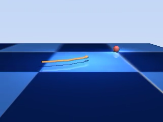
(b) swimmer
$n=16\,m=5$

(c) walker
$n=18\,m=6$

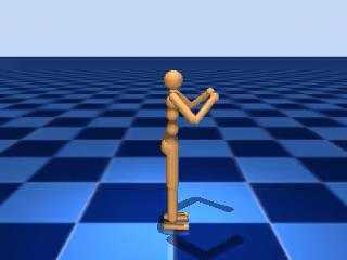
(d) humanoid
$n=55\,m=21$

Figure 1: Visualization of robots used in the experiments.

III Experiments

We compare our method (LaLQR) against: nonlinear MPC (SQP) and imitation learning (IL) on 4 robotic tasks as in Figure 1 based on the simulated platform MuJoCo [8]. Table I shows that for control efficiency, both LaLQR and IL require much less computational time compared with the original SQP controller. LaLQR achieves competitive or excelling control results compared with IL for all tasks. Its total cost even approaches SQP for cartpole and swimmer.

TABLE I: Testing results on $4$ simulated robotic tasks.

Tasks		SQP	IL	LaLQR (Ours)
cartpole	total_cost	$3042.56\pm 2156.08$	$3121.99\pm 2115.25$	$3141.30\pm 1815.42$
	average_time	$10.26\pm 0.42$	$0.25\pm 0.07$	$0.24\pm 0.05$
swimmer	total_cost	$365.07\pm 9.55$	$419.54\pm 9.41$	$418.63\pm 6.81$
	average_time	$43.88\pm 2.90$	$0.34\pm 0.10$	$0.32\pm 0.09$
walker	total_cost	$2.92\pm 0.03$	$107.47\pm 0.36$	$30.15\pm 0.16$
	average_time	$20.53\pm 1.41$	$0.47\pm 0.12$	$0.44\pm 0.06$
humanoid	total_cost	$194.57\pm 46.90$	$22606.60\pm 70.25$	$790.85\pm 58.81$
	average_time	$44.36\pm 8.37$	$5.49\pm 2.00$	$5.48\pm 1.88$

References

- [1] J. Di Carlo, P. M. Wensing, B. Katz, G. Bledt, and S. Kim, “Dynamic locomotion in the mit cheetah 3 through convex model-predictive control,” in 2018 IEEE/RSJ International Conference on Intelligent Robots and Systems (IROS). Madrid: IEEE, Oct. 2018, pp. 1–9.
- [2] R. Grandia, F. Jenelten, S. Yang, F. Farshidian, and M. Hutter, “Perceptive locomotion through nonlinear model-predictive control,” IEEE Trans. Robotics, vol. 39, no. 5, pp. 3402–3421, 2023.
- [3] Y. Song and D. Scaramuzza, “Learning high-level policies for model predictive control,” in 2020 IEEE/RSJ International Conference on Intelligent Robots and Systems (IROS), Oct. 2020, pp. 7629–7636.
- [4] M. Diehl, H. J. Ferreau, and N. Haverbeke, “Efficient numerical methods for nonlinear mpc and moving horizon estimation,” in Nonlinear Model Predictive Control, M. Morari, M. Thoma, L. Magni, D. M. Raimondo, and F. Allgöwer, Eds. Berlin, Heidelberg: Springer Berlin Heidelberg, 2009, vol. 384, pp. 391–417.
- [5] S. L. Brunton, M. Budisic, E. Kaiser, and J. N. Kutz, “Modern koopman theory for dynamical systems,” SIAM Rev., vol. 64, no. 2, pp. 229–340, 2022.
- [6] P. J. Antsaklis and A. N. Michel, A Linear Systems Primer. Springer Science & Business Media, 2007.
- [7] B. D. Anderson and J. B. Moore, Optimal Control: Linear Quadratic Methods. Courier Corporation, 2007.
- [8] E. Todorov, T. Erez, and Y. Tassa, “Mujoco: A physics engine for model-based control,” in 2012 IEEE/RSJ International Conference on Intelligent Robots and Systems. Vilamoura-Algarve, Portugal: IEEE, Oct. 2012, pp. 5026–5033.