Multipole responses in fissioning nuclei and their uncertainties

Abstract

Electromagnetic multipole responses are key inputs to model the structure, decay and reaction of atomic nuclei. With the introduction of the finite amplitude method (FAM), large-scale calculations of the nuclear linear response in heavy deformed nuclei have become possible. This work provides a detailed study of multipole responses in actinide nuclei with Skyrme energy density functionals. We quantify both systematic and statistical uncertainties induced by the functional parameterization in FAM calculations. We also extend the FAM formalism to perform blocking calculations with the equal filling approximation for odd-mass and odd-odd nuclei, and analyze the impact of blocking configurations on the response. By examining the entire plutonium isotopic chain from the proton to the neutron dripline, we find a large variability of the response with the neutron number and study how it correlates with the deformation of the nuclear ground state.

I Introduction

Photonuclear processes are amongst the most valuable probes into the structure and reactions of atomic nuclei. Electromagnetic transitions between discrete low-lying excited states are used to reconstruct the excitation spectrum of the nucleus with the help of coincidence techniques [1, 2]. At higher energies, the emission of photons becomes statistical and is typically quantified by the $\gamma$-strength function ($\gamma$SF) [3]. Invoking the Brink-Axel hypothesis [4, 5] allows using these $\gamma$SFs to characterize the absorption of a photon by the nucleus in statistical reaction theory. As such, they play an essential role both in fundamental physics such as nucleosynthesis, or in applications ranging from medical isotope production to fission technology and nuclear forensics.

Discrete electromagnetic transitions can be computed directly as the matrix elements of relevant operators – the multipole operators of the electromagnetic field – between initial and final nuclear states. Configuration-interaction (CI) methods such as the nuclear shell model are well suited to this task [6]. The shell model can also be used to compute $\gamma$SFs in selected mass regions thanks to averaging procedures [7, 8, 9]. In heavy deformed nuclei, direct CI methods often become impractical and microscopic calculations of electromagnetic transitions are performed with collective models such as the Bohr Hamiltonian [10, 11] or within symmetry-conserving, multi-reference energy density functional theory; see, e.g., [12, 13, 14, 15, 16, 17] for a selection of relatively recent applications. To compute $\gamma$SFs, the linear response theory based on the quasiparticle random phase approximation (QRPA) remains by far the most common approach; see, e.g., [18, 19, 20, 21, 22, 23, 24, 25] for examples of such studies with Skyrme, Gogny, and covariant energy functionals. Theories going beyond the linear response have only been applied on a case-by-case basis as they are computationally a lot more expensive [26, 27, 28, 29, 30, 31, 32, 33, 34].

For a long time, fully self-consistent QRPA calculations in heavy deformed nuclei were hampered by their large computational costs [35, 36, 37]. However, the invention of the finite-amplitude method (FAM) made calculations of the linear response in such nuclei much more accessible [38, 39, 40]. The focus of early studies on the FAM was largely to establish benchmarks against the direct QRPA [41, 42, 43, 44] and probe its feasibility and predictive power for multipole responses or photoabsorption cross sections [45, 46]. The goal of this paper is to apply the finite amplitude method to perform a more systematic analysis of the multiple response in actinide nuclei. In particular, we pay special attention to estimating theoretical uncertainties originating from the parameterization of the energy functional and test the extension of the FAM for odd-mass and odd-odd nuclei. This work is a prelude to a more large-scale calculation of $\gamma$SFs at the scale of the entire mass table.

This paper is organized as follows. In Sec. II we briefly summarize the like-particle FAM formalism for electromagnetic operators. The numerical setup of our calculations is presented in Sec. III. Benchmark calculations of photoabsorption cross sections and electromagnetic multipole responses are shown in Sec. IV with detailed analyses of their uncertainties. Properties of electromagnetic responses in actinides nuclei are then discussed in Sec. V. Additional technical details, such as the quasiparticle cutoff procedure used in the calculation of transition densities and equations for energy-weighted sum rules, are given in the Appendices; additional figures and tables are provided in the Supplemental Material [47].

II Theoretical Framework

The FAM formalism for an even-even nucleus was presented in Refs. [38, 39], and its extension to odd-$A$ and odd-odd nuclei for $\beta$-decay calculations was published in Ref. [48], followed by Ref. [49] for the applications of the finite-temperature (FT) FAM on electron capture. In Sec. II.1 we give a unified summary of the FAM that incorporates the cases of even-even, odd-$A$ and odd-odd nuclei, as well as the FT system. In Sec. II.2, we provide formulas relevant to the application of the FAM to electromagnetic responses.

II.1 Finite amplitude method

In the FAM, an external perturbation is applied on a nucleus to induce oscillations around a static Hartree-Fock-Bogoliubov (HFB) state, which can be described by the small-amplitude limit of the time-dependent HFB (TDHFB) equation. The HFB state of an even-even nucleus is a vacuum with respect to Bogoliubov quasiparticle operators, i.e., $\beta_{\mu}|\Phi\rangle=0$. To compute an odd-$A$ nucleus, we employ the equal filling approximation (EFA) [50, 51, 52] to preserve the time-reversal symmetry in the static HFB calculation. In the EFA, all the densities are computed by averaging the densities of the one-quasiparticle state $\beta^{\dagger}_{\mu_{B}}|\Phi\rangle$ and its time-reversed partner $\beta^{\dagger}_{\bar{\mu}_{B}}|\Phi\rangle$. An odd-odd nucleus can be similarly described by averaging the densities of a two-quasiparticle state and its time-reversed partner. The EFA-HFB state can be treated as a special case of the FT-HFB state [51]. Both of them can be described as a statistical ensemble whose density operator is

$$\hat{\mathcal{D}}= |\Phi\rangle\langle\Phi|+\sum_{\mu}\beta_{\mu}^{\dagger}|\Phi\rangle p_{\mu}\langle\Phi|\beta_{\mu}$$ (1)

$$+\frac{1}{2!}\sum_{\mu\nu}\beta_{\mu}^{\dagger}\beta_{\nu}^{\dagger}|\Phi\rangle p_{\mu}p_{\nu}\langle\Phi|\beta_{\nu}\beta_{\mu}+\cdots,$$

where $p_{\mu}=\frac{f_{\mu}}{1-f_{\mu}}$ and $f_{\mu}$ is the quasiparticle occupancy. In the EFA the occupancy $f_{\mu}$ is

$$f_{\mu}=\begin{cases}\frac{1}{2}&\mu=\mu_{B}\text{ or }\bar{\mu}_{B},\\ 0&\text{otherwise},\end{cases}$$ (2)

while in the FT-HFB calculation it is given by the Fermi-Dirac distribution

$$f_{\mu}=\frac{1}{e^{E_{\mu}/(k_{B}T)}+1},$$ (3)

where $E_{\mu}$ is the quasiparticle energy and $T$ is the temperature. The corresponding generalized density matrix is

$$\mathbb{R}_{\mu\nu}=\begin{pmatrix}\langle\beta^{\dagger}_{\nu}\beta_{\mu}\rangle&\langle\beta_{\nu}\beta_{\mu}\rangle\\ \langle\beta^{\dagger}_{\nu}\beta^{\dagger}_{\mu}\rangle&\langle\beta_{\nu}\beta^{\dagger}_{\mu}\rangle\end{pmatrix}=\begin{pmatrix}f_{\mu}\delta_{\mu\nu}&0\\ 0&1-f_{\mu}\delta_{\mu\nu}\end{pmatrix}.$$ (4)

We see that an even-even nucleus can also be treated as a statistical ensemble with $f_{\mu}=0$ for all the quasiparticles. It should be noted that all the discussions above apply to both static and time-dependent HFB states.

In the FAM we assume that the nucleus oscillates under a weak external field of frequency $\omega$:

$$F(t)=\eta\Big{[}F(\omega)e^{-i\omega t}+F^{\dagger}(\omega)e^{i\omega t}\Big{]},$$ (5)

where $\eta$ is a small real number and

$$F(\omega)=\frac{1}{2}\sum_{\mu\nu}\left(F_{\mu\nu}^{20}A_{\mu\nu}^{\dagger}+F_{\mu\nu}^{02}A_{\mu\nu}\right)+\sum_{\mu\nu}F_{\mu\nu}^{11}B_{\mu\nu},$$ (6)

where $A^{\dagger}_{\mu\nu}\equiv\beta^{\dagger}_{\mu}\beta^{\dagger}_{\nu}$, $B_{\mu\nu}\equiv\beta^{\dagger}_{\mu}\beta_{\nu}$, and $F^{20}$ and $F^{02}$ are antisymmetric matrices. As shown in [53], taking into account this time-dependent operator into the TDHFB equation results in small oscillations of the TDHFB mean field:

$$\mathcal{H}(t) =\mathcal{H}_{0}+\eta\Big{[}\delta\mathcal{H}(\omega)e^{-i\omega t}+\delta\mathcal{H}^{\dagger}(\omega)e^{i\omega t}\Big{]},$$ (7a)

$$\delta\mathcal{H}(\omega) =\frac{1}{2}\sum_{\mu\nu}\left(\delta H_{\mu\nu}^{20}A_{\mu\nu}^{\dagger}+\delta H_{\mu\nu}^{02}A_{\mu\nu}\right)+\delta H_{\mu\nu}^{11}B_{\mu\nu},$$ (7b)

where $\mathcal{H}_{0}=\sum_{\mu}E_{\mu}B_{\mu\mu}$ is the static HFB Hamiltonian. The time-dependent quasiparticle operator can be decomposed in a similar manner as

$$\beta_{\mu}(t)=\Big{[}\beta_{\mu}+\eta\delta\beta_{\mu}(t)\Big{]}e^{iE_{\mu}t},$$ (8)

where $\beta_{\mu}$ is the quasiparticle operator of the static HFB solution, and $\delta\beta_{\mu}(t)$ can be written as

$$\delta\beta_{\mu}(t)= \sum_{\nu}\beta_{\nu}^{\dagger}\Big{[}X_{\nu\mu}(\omega)e^{-i\omega t}+Y_{\nu\mu}^{*}(\omega)e^{i\omega t}\Big{]}$$ (9)

$$+\sum_{\nu}\beta_{\nu}\Big{[}P_{\mu\nu}(\omega)e^{-i\omega t}+Q^{*}_{\mu\nu}(\omega)e^{i\omega t}\Big{]},$$

where $X$, $Y$, $P$ and $Q$ are called FAM amplitudes. Using the unitarity of the Bogoliubov transformation, we can prove $Q=-P^{T}$ while $X$ and $Y$ are antisymmetric; see Appendix A for details.

We can substitute the expressions of $F(t)$, $\mathcal{H}(t)$ and $\beta_{\mu}(t)$ into the TDHFB equation to get

$$i\frac{\partial\beta_{\mu}(t)}{\partial t}=\left[\mathcal{H}(t)+F(t),\beta_{\mu}(t)\right],$$ (10)

where we use $\hbar=1$. Expanding Eq. (10) up to the first order in $\eta$, we obtain the FAM equations

$$\left(E_{\mu}-E_{\nu}-\omega\right)P_{\mu\nu}(\omega)-\delta H^{11}_{\mu\nu}(\omega)-F^{11}_{\mu\nu} =0,$$ (11a)

$$\left(E_{\mu}+E_{\nu}-\omega\right)X_{\mu\nu}(\omega)+\delta H^{20}_{\mu\nu}(\omega)+F^{20}_{\mu\nu} =0,$$ (11b)

$$\left(E_{\mu}+E_{\nu}+\omega\right)Y_{\mu\nu}(\omega)+\delta H^{02}_{\mu\nu}(\omega)+F^{02}_{\mu\nu} =0.$$ (11c)

Expanding the induced mean field $\delta H$ in terms of the FAM amplitudes $(P,X,Y)$ yields the FT-QRPA equation presented in Ref. [54].

Constructing the matrix involved in the FT-QRPA equation is numerically very expensive since it has a dimension of $4\times N_{2\mathrm{qp}}$, where $N_{2\mathrm{qp}}$ is the number of two-quasiparticle excitations: in heavy nuclei where there could be about $10^{3}$ relevant quasiparticles, this leads to a QRPA matrix with a dimension of order $10^{6}$, that is, about $10^{12}$ matrix elements to compute. In the FAM, we calculate the induced densities listed in Appendix B from the FAM amplitudes to determine the induced mean fields (7), which allows solving the FAM equations (11). This procedure is iterative but avoids explicitly building the FT-QRPA matrix, which significantly accelerates the calculation. In Appendix B we provide more details about the induced densities and mean fields, and show why the amplitude $P$ does not contribute in an even-even nucleus. We also discuss how to implement the quasiparticle cutoff to avoid the ultra-violet divergence brought by zero-range pairing interactions [55, 56, 57].

II.2 Transition strength and electromagnetic transition operators

Using the solutions of Eq. (11), we can compute the transition strength distribution [38, 39]

$$\frac{dB(\omega;F)}{d\omega}=\sum_{n>0}|\langle n|F|0\rangle|^{2}\delta\left(\omega-\Omega_{n}\right)=-\frac{1}{\pi}\operatorname{Im}S(\omega;F),$$ (12)

where $\Omega_{n}$ is the excitation energy of $|n\rangle$ and $S(\omega;F)$ is the FAM response function given by

$$S(\omega;F)=\mathrm{Tr}\left(f^{\dagger}\delta\rho\right)=\sum_{kl}f^{*}_{kl}\delta\rho_{kl}(\omega;F),$$ (13)

where $f_{kl}$ are the matrix elements of the external field in the single-particle (s.p.) basis ($F(\omega)=\sum_{kl}f_{kl}c^{\dagger}_{k}c_{l}$), and the induced density matrix $\delta\rho$ is given by Eq. (45). In practical calculations, we usually adopt a complex frequency $\omega\rightarrow\omega+i\gamma$, and the corresponding strength distribution is smeared by a Lorentzian function with a half width $\gamma$ (full width $\Gamma=2\gamma$):

$$\frac{dB}{d\omega}=\frac{\gamma}{\pi}\sum_{n}\left\{\frac{|\langle n|F|0\rangle|^{2}}{\left(\omega-\Omega_{n}\right)^{2}+\gamma^{2}}-\frac{|\langle n|F^{\dagger}|0\rangle|^{2}}{\left(\omega+\Omega_{n}\right)^{2}+\gamma^{2}}\right\}.$$ (14)

The smearing width $\gamma$ mainly accounts for the spreading effect brought by mode-mode coupling [58]. In linear response theory where such coupling effects are not computed, the smearing width should in principle be adjusted to match experimental evaluations [59]. In this paper we adopt a standard width of $\Gamma=1$ MeV, unless otherwise stated, and perform FAM calculations on a $\omega$ grid with 0.1 MeV spacing, which is fine enough for $\Gamma=1$ MeV.

In this work we study electromagnetic multipole transitions in heavy nuclei. The electric multipole transition operator is written in spherical coordinates as [60]

$$Q_{LK}=e\sum_{i=1}^{A}q_{\tau_{i}}r_{i}^{L}Y_{LK}(\Omega_{i}),$$ (15)

where particle $i$ is either a neutron ($\tau_{i}=n$) or a proton ($\tau_{i}=p$), $q_{\tau}$ is the effective charge in the unit of the elementary charge $e$, $\Omega_{i}\equiv(\theta_{i},\varphi_{i})$ are the angular coordinates, and $Y_{LK}(\Omega_{i})$ the spherical harmonics [61]. The magnetic multipole operator is [60]

$$M_{LK}=\mu_{\mathrm{N}}\sum_{i=1}^{A}\bm{\nabla}\left[r_{i}^{L}Y_{LK}(\Omega_{i})\right]\cdot\left(\frac{2g_{l}^{(\tau_{i})}}{L+1}\bm{l}_{i}+g_{s}^{(\tau_{i})}\bm{s}_{i}\right),$$ (16)

where $\mu_{N}$ is the nuclear magneton, $\bm{l}_{i}=\left(\bm{r}_{i}\times\bm{p}_{i}\right)/\hbar$ the orbital angular-momentum operator, $\bm{s}_{i}=\frac{1}{2}\bm{\sigma_{i}}$ the spin operator, and $g_{l}^{(\tau)}$ and $g_{s}^{(\tau)}$ are the effective $g$ factors of a nucleon of type $\tau$. In this paper we use the bare charges and bare $g$ factors of nucleons in multipole operators $Q$ and $M$, i.e., we take $q_{n}=0$, $q_{p}=1$, $g_{l}^{(n)}=0$, $g_{l}^{(p)}=1$, $g_{s}^{(n)}=5.586$, and $g_{s}^{(p)}=-3.826$ [62]. It has been suggested that the spin $g$ factors be quenched to match the calculations of $M1$ responses with experimental data [58]; this problem is beyond the scope of this paper. In addition, we decompose the multipole operator $V=Q$ or $M$ into isoscalar (IS) and isovector (IV) components as

$$V=\frac{1}{2}\left(V^{\mathrm{IS}}+V^{\mathrm{IV}}\right),$$ (17)

where neutrons and protons take equal (opposite) effective charges or $g$ factors in $V^{\mathrm{IS}}$ ($V^{\mathrm{IV}}$).

For the electric dipole ($E1$) operator, we can explicitly remove the center-of-mass motion and obtain following effective charges [60]

$$q_{n}=-\frac{Z}{A},\quad q_{p}=\frac{N}{A}.$$ (18)

One can see that when $N=Z$ the $E1$ operator becomes purely isovector. When $N$ and $Z$ do not differ much, the $E1$ operator is mostly isovector and the corresponding response will heavily depend on the isovector component of the energy density functional (EDF).

With the $E1$ operator, we can calculate the cross section for the absorption of dipole radiation. Assuming that incoming photons with energy $\omega$ come along the $z$ axis in the lab frame, the $E1$ photoabsorption cross section is [60]

$$\sigma_{\rm abs}(\omega)=\frac{16\pi^{3}}{3}\alpha\sum_{n>0}\omega\left|\langle\Psi_{n}|Q_{10}^{\mathrm{eff}}|\Psi_{0}\rangle\right|^{2}\delta(\omega-\Omega_{n}),$$ (19)

where $\alpha=\frac{e^{2}}{\hbar c}$ is the fine structure constant, $|\Psi_{0}\rangle$ is the ground state and $|\Psi_{n}\rangle$ the $n^{\rm th}$ excited state, both in the laboratory frame, and $\Omega_{n}$ is the excitation energy. The superscript “eff” on $Q_{1K}$ denotes the use of effective charges given in Eq. (18). In this work we ignore the contributions from magnetic and high-order electric transitions to the photoabsorption cross section, since they are usually much smaller than that from the $E1$ transition [63].

For a deformed nucleus, both HFB and FAM calculations are carried out in the intrinsic frame of the nucleus, so we need to perform angular-momentum projection (spherical symmetry restoration) [60, 64, 65] to obtain wavefunctions in the laboratory frame. After projection, the $E1$ photoabsorption cross section (19) can be expressed as [40, 59, 46]

$$\sigma_{\rm abs}(\omega)=\frac{16\pi^{3}}{9}\alpha\sum_{K=0,\pm 1}\frac{dB(\omega;Q_{1K}^{\mathrm{eff}})}{d\omega},$$ (20)

where $dB/d\omega$ is evaluated in the intrinsic frame via Eqs. (12) and (13). One can find more details in Ref. [65] on the angular-momentum projection in QRPA and FAM calculations.

When the static HFB solution is time-reversal invariant, the FAM responses of multipole operators $V_{LK}$ and $V_{L-K}$ are equal: only the results of $K=0$ and $1$ in Eq. (20) need to be calculated. When the static HFB solution has spherical symmetry, the FAM response will not depend on $K$, and we can thus further reduce the computational cost.

III Numerical Setup

With the formalism presented in Sec. II, we have developed a new numerical program called gfam to perform axially-deformed FAM calculations with Skyrme EDFs for nuclear electromagnetic transitions. gfam is based on the charge-changing FAM code pnfam [66, 48, 49], which was successfully employed to conduct global calculations on the $\beta$ decay of even-even, odd-$A$ and odd-odd nuclei [67, 68], as well as the finite-temperature electron capture [49]. Like pnfam, the gfam program is also computationally efficient and amenable to large-scale studies. One of its inputs is the static HFB solution from the hfbtho code [69, 70, 71, 72].

In our HFB and FAM calculations, all the quasiparticle wavefunctions are expanded in a deformed harmonic-oscillator (HO) basis up to $N_{0}=20$ shells. The oscillator length is given by the default setting in hfbtho [70]. We also vary the quadrupole deformation $\beta_{2}$ of the HO basis and initial constraint between -0.2 and 0.2 to locate the HFB ground state. In the particle-particle channel we use a mixed surface-volume delta force, with a pairing cutoff of $E_{\rm cut}=60$ MeV [73]. With the numerical parameters given above, it takes less than an hour on a node with 56 CPU cores to solve the FAM equations over 500 $\omega$ points, which is fast enough for future surveys over the nuclear chart. One can find discussions in Ref. [74] about the dependence of FAM responses on various numerical parameters.

In this work, we consider several Skyrme EDFs fitted under various protocols to show the systematic uncertainties of FAM results. The SLy4 (without tensor terms) and SLy5 (with tensor terms) functionals were fitted to improve the description of neutron-rich nuclei and included a constraint on the Thomas-Reiche-Kuhn (TRK) sum rule [75]. The SkM* parametrization is the reference EDF for the studies of deformed nuclei, especially nuclear fission [76]. The SkI3 functional was fitted largely to improve the description of the isotope shifts in the Pb region [77]. Finally, the HFB1 (UNEDF1-HFB) functional is the only one in our set where the particle-particle channel is fitted simultaneously with the particle-hole channel [78]. It is similar to the UNEDF1 functional [79], only without the Lipkin-Nogami prescription for pairing. These EDFs predict a relativey broad range of nuclear matter properties as shown in Table 1, where we follow the notations of Ref. [80].

Table 1: Summary of nuclear matter properties for the five energy functionals considered in this work. The saturation density $\rho_{\rm c}$ is in fm^-3; the binding energy per nucleon $E^{\text{NM}}/A$, incompressibility $K^{\text{NM}}$, symmetry energy $a_{\text{sym}}^{\text{NM}}$ are in MeV; the isoscalar effective mass $M_{s}^{*}$ and enhancement factor of the Thomas-Reiche-Kuhn sum rule $\kappa_{\rm TRK}$ (26) are dimensionless.

	$\rho_{\rm c}$	$E^{\text{NM}}/A$	$K^{\text{NM}}$	$M_{s}^{*}$	$a_{\text{sym}}^{\text{NM}}$	$\kappa_{\rm TRK}$
SLy4	0.160	-15.97	229.90	0.694	32.00	0.250
SLy5	0.160	-15.98	229.91	0.698	32.01	0.250
SkM*	0.160	-15.77	216.66	0.786	30.03	0.532
SkI3	0.158	-15.96	257.97	0.577	34.83	0.245
HFB1	0.156	-15.80	244.84	0.936	28.67	0.250

The SLy4, SLy5, SkM* and SkI3 parameterizations only determine the Skyrme functional in the particle-hole channel and specify neither the form nor the parameters of the pairing functional. As mentioned earlier, we use a pairing functional derived from a density-dependent pairing force with mixed surface-volume nature, which is controlled by two pairing strengths $V_{0}^{n}$ and $V_{0}^{p}$ for neutrons and protons, respectively. Following the procedure of Ref. [81], we fit these pairing strengths to reproduce the 3-point formula for the odd-even mass staggering of ²³²Th.

Since the time-reversal symmetry is broken in the FAM calculation, we need to consider Skyrme-EDF terms involving time-odd densities:

$$\chi_{tt_{3}}^{\mathrm{(odd)}}= C_{t}^{s}\bm{s}_{tt_{3}}^{2}+C_{t}^{\Delta s}\bm{s}_{tt_{3}}\cdot\nabla^{2}\bm{s}_{tt_{3}}+C_{t}^{j}\bm{j}_{tt_{3}}^{2}$$ (21)

$$+C_{t}^{\nabla j}\bm{s}_{tt_{3}}\cdot\nabla\times\bm{j}_{tt_{3}}+C_{t}^{T}\bm{s}_{tt_{3}}\cdot\bm{T}_{tt_{3}}$$

$$+C_{t}^{F}\bm{s}_{tt_{3}}\cdot\bm{F}_{tt_{3}}+C_{t}^{\nabla s}\left(\nabla\cdot\bm{s}_{tt_{3}}\right)^{2},$$

where we follow the notations given in Ref. [82]. For SLy4, SLy5, SkM* and SkI3, all coupling constants $C_{t}^{u}$ are computed from the Skyrme force parameters $(t,x)$ [82]. For HFB1, however, only time-even Skyrme couplings are provided in [78]. We thus first transform these time-even couplings into $(t,x)$ parameters and then obtain time-odd couplings from $(t,x)$ [57]. Furthermore, in our calculations we set $C^{\Delta s}_{t}=0$ to avoid finite-size instabilities [83, 84, 52, 85, 86]. While this latter choice has very little impact on FAM calculations with SLy4, SLy5, SkI3 and SkM*, both in terms of convergence and the values of final results, we find that it greatly improves the convergence of calculations with HFB1 without significantly changing the results.

Besides the systematic uncertainties, we also study the statistical uncertainties of FAM calculations with samples generated from Bayesian model calibration. We first calibrate the HFB1 functional following the procedure presented in Refs. [87, 88, 89], using the the probabilistic programming language Stan [90]; the posterior distribution obtained from the calibration is presented in the Supplemental Material [47]. We then propagate the uncertainties of Skyrme parameters to FAM responses by carrying out FAM calculations with 50 samples taken inside the 95% credible region of the posterior distribution.

IV Multipole Responses in Selected Even-Even Nuclei

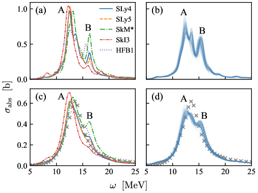
Figure 1: Panel (a): photoabsorption cross sections of ²⁰⁸Pb as functions of the photon energy $\omega$, calculated with different Skyrme parameterizations and a width of $\Gamma=1$ MeV. Panel (b): similar to panel (a) but calculated with the 50 samples from the HFB1 posterior distribution. Panels (c) and (d): similar to panels (a) and (b) but calculated with a width of $\Gamma=2$ MeV. The evaluated nuclear data [91] are shown by cross markers.

To benchmark our new code we first perform calculations for the multipole responses in doubly magic nucleus ²⁰⁸Pb, semi-magic spherical nucleus ⁹⁰Zr, and axially deformed nucleus ²⁴⁰Pu. Our results are consistent with previous FAM calculations [45], which validates the correctness of gfam. In the following we will analyze the systematic and statistical uncertainties of the multipole responses in these even-even nuclei.

IV.1 $E1$ transition

Table 2 lists the giant dipole resonance (GDR) energies of ⁹⁰Zr and ²⁰⁸Pb obtained from FAM calculations for the $E1$ transition. The mean value and standard deviation of the resonance energies obtained from calculations with SLy4, SLy5, SkM*, SkI3 and HFB1 are taken as the systematic mean, $\bar{x}_{\rm sys}$, and uncertainty, $\sigma_{\rm sys}$, respectively, while the statistical mean value $\bar{x}_{\rm stat}$ and standard deviation $\sigma_{\rm stat}$ are obtained from the posterior samples of Skyrme parameters generated by the Bayesian model calibration for HFB1. We see that the calculated GDR energies of ⁹⁰Zr and ²⁰⁸Pb are close to their corresponding experimental values. Besides, the systematic uncertainty of the GDR energy of ⁹⁰Zr is much larger than the statistical one, while the two uncertainties for ²⁰⁸Pb are almost equal.

Table 2: Giant dipole resonance (GDR) energies of ⁹⁰Zr and ²⁰⁸Pb, and giant quadrupole resonance (GQR) energies of ²⁰⁸Pb obtained from FAM calculations with various Skyrme EDFs. For the GQR both isoscalar (IS) and isovector (IV) resonance energies are given. The systematic mean value $\bar{x}_{\rm sys}$ and standard deviation $\sigma_{\rm sys}$ are obtained from the results with SLy4, SLy5, SkM*, SkI3 and HFB1 functionals. The statistical mean value $\bar{x}_{\rm stat}$ and standard deviation $\sigma_{\rm stat}$ are obtained from the 50 HFB1 posterior samples. Experimental values for the GDR energies are the averages of the data given in Table 1 of [92]; the ISGQR and IVGQR energies are taken from [93].

	$E_{\rm GDR}$(90Zr)	$E_{\rm GDR}$(208Pb)	$E_{\rm ISGQR}$	$E_{\rm IVGQR}$
exp	$16.8$	$13.4$	$10.9$	$22.7$
SLy4	$15.6$	$12.5$	$12.3$	$22.7$
SLy5	$15.5$	$12.5$	$12.2$	$22.8$
SkM*	$17.5$	$13.1$	$11.5$	$22.4$
SkI3	$16.1$	$12.2$	$13.5$	$21.8$
HFB1	$17.2$	$12.6$	$10.7$	$22.0$
$\bar{x}_{\rm sys}$	$16.4$	$12.6$	$12.0$	$22.3$
$\sigma_{\rm sys}$	$0.8$	$0.3$	$0.9$	$0.4$
$\bar{x}_{\rm stat}$	$17.0$	$12.5$	$12.0$	$21.9$
$\sigma_{\rm stat}$	$0.1$	$0.3$	$0.1$	$0.4$

Figure 1 shows the photoabsorption cross sections of ²⁰⁸Pb calculated with different Skyrme EDFs and widths $\Gamma=1$ and 2 MeV. First, we see that the cross sections obtained with different parameterizations show similar patterns. The position of the giant resonance marked by “A” in Fig. 1 does not vary significantly when we change the underlying Skyrme EDF, but its height can differ dramatically, especially between HFB1 and other EDFs in panels (a, c) and among the statistical samples in panels (b, d). Second, the peak marked by “B” in Fig. 1 vary a lot in panels (a, c) as we change the underlying EDF; its statistical uncertainty shown in panels (b, d), however, is smaller than the systematic one.

We obtain good agreement with the nuclear data evaluation [91] when we take a larger width ($\Gamma=2$ MeV). The major difference is that the peak “B” (shoulder structure) in Fig. 1 does not exist in the evaluation. This shoulder was also observed in previous calculations [94, 95] and was attributed to the intruder state with a large angular momentum [94]. The dependence of peak “B” on the s.p. structure can explain why it is more sensitive to the choice of the Skyrme parameterization than the collective resonance “A”.

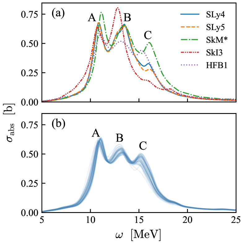
Figure 2: Similar to panels (a) and (b) of Fig. 1 but for ²⁴⁰Pu.

The photoabsorption cross section of ²⁴⁰Pu is displayed in Fig. 2. As expected, we observe that the ground-state deformation of this nucleus causes significant fragmentation of the transition strength distribution. The peak “A” in Fig. 2 is given by the FAM calculation of $K=0$ and depends weakly on the Skyrme EDF (the only outlier is SKM*). The peaks “B” and “C”, however, are quite sensitive to the Skyrme parameterizations, and their systematic uncertainties are much greater than statistical ones. Both “B” and “C” peaks originate from the strength distribution of $|K|=1$. Since the ground state of ²⁴⁰Pu has a prolate shape, the effective oscillator length along the $z$ axis ($K=0$) is longer than that along the $x$ or $y$ axis ($|K|=1$), and thus the peak “A” has a lower energy than peaks “B” and “C”.

Interestingly, the variations shown in Figs. 1 and 2 are not strongly correlated with the bulk properties of static HFB states: the systematic uncertainty of the HFB energy of ²⁴⁰Pu is 4.6 MeV, which is much smaller than the statistical uncertainty 12.3 MeV. However, the photoabsorption cross section shows an opposite trend: in Figs. 1 and 2 the systematic uncertainty is much larger than the statistical one. This offers conclusive evidence that observables related to nuclear electromagnetic transitions can provide information that is not captured by the fits of EDFs with ground-state properties only.

IV.2 Sum rules

To better understand the variations of the photoabsorption cross sections discussed in the previous section, we study the systematic and statistical uncertainties of sum rules [96, 63, 60]

$$m_{k}(F)=\int\omega^{k}\frac{dB(\omega;F)}{d\omega}d\omega=\sum_{n>0}\Omega_{n}^{k}\left|\left\langle n|F|0\right\rangle\right|^{2}.$$ (22)

We first look into the energy-weighted sum rule $m_{1}$, which can be evaluated with the Hamiltonian $H$ and static HFB state $|0\rangle$ as [97, 98, 96, 63, 60, 99, 44]

$$m_{1}(F)=\frac{1}{2}\langle 0|[F^{\dagger},[H,F]]|0\rangle=(1+\kappa)m_{1}^{T}(F),$$ (23)

where $m_{1}^{T}$ is given by the double commutator involving the kinetic-energy term only, and $\kappa$ is the enhancement factor due to the momentum dependence of the effective interaction. For the Skyrme EDF, the expressions of $m_{1}$ for electric multipole operators are presented in Appendix C, based on which we can obtain the TRK sum rule for the $E1$ transition as [63, 60, 46]

$$m_{1}(E1)=\frac{e^{2}\hbar^{2}}{2m}\left[1+\kappa(E1)\right]\frac{NZ}{A}\frac{3}{4\pi},$$ (24)

where the enhancement factor $\kappa(E1)$ is the only component that depends on the static HFB solution

$$\kappa(E1)=\frac{2m}{\hbar^{2}}\frac{A}{NZ}\left(C^{\tau}_{0}-C^{\tau}_{1}\right)\int\rho_{n}(\bm{r})\rho_{p}(\bm{r})d\bm{r},$$ (25)

where $\rho_{n}$ and $\rho_{p}$ are neutron and proton densities of the HFB ground state, and $C^{\tau}_{t}$ is the coupling constant of the term $\rho_{t}\tau_{t}$ in the Skyrme EDF. Based on Eq. (25), we can write the TRK enhancement factor in symmetric nuclear matter as [100, 46]

$$\kappa_{\rm TRK}=\frac{2m}{\hbar^{2}}\left(C^{\tau}_{0}-C^{\tau}_{1}\right)\rho_{c}=M_{v}^{*-1}-1,$$ (26)

where $\rho_{c}$ is the saturation density and $M_{v}^{*}$ is the isovector effective mass in the unit of the nucleon mass $m$. The ratio of enhancement factors (25) and (26) is then

$$\frac{\kappa(E1)}{\kappa_{\rm TRK}}=\frac{A}{NZ\rho_{c}}\int\rho_{n}(\bm{r})\rho_{p}(\bm{r})d\bm{r}.$$ (27)

Table 3 lists the energy-weighted sum rules and enhancement factors for the $E1$ transition in ²⁰⁸Pb, obtained from static HFB solutions calculated with various Skyrme EDFs. Integrating the energy-weighted FAM strength distributions up to 50 MeV can give 96% to 98% of the sum rules presented in Table 3.

Table 3: Energy-weighted sum rules $m_{1}(E1)$ (23), enhancement factors $\kappa(E1)$ (25) and $\kappa_{\rm TRK}$ (26), and their ratios (27) in ²⁰⁸Pb. All the values are obtained from the HFB ground states calculated with various Skyrme EDFs. See the caption of Table 2 for the definitions of $\bar{x}$ and $\sigma$.

	$m_{1}(E1)$	$\kappa(E1)$	$\kappa_{\rm TRK}$	$\kappa(E1)/\kappa_{\rm TRK}$
SLy4	$2.909$	$0.189$	$0.250$	$0.750$
SLy5	$2.910$	$0.189$	$0.250$	$0.760$
SkM*	$3.428$	$0.401$	$0.532$	$0.750$
SkI3	$2.920$	$0.187$	$0.245$	$0.760$
HFB1	$2.933$	$0.193$	$0.250$	$0.770$
$\bar{x}_{\rm sys}$	$3.020$	$0.232$	$0.305$	$0.758$
$\sigma_{\rm sys}$	$0.204$	$0.085$	$0.113$	$0.007$
$\bar{x}_{\rm stat}$	$2.935$	$0.194$	$0.250$	$0.780$
$\sigma_{\rm stat}$	$0.005$	$0.002$	$0.000$	$0.008$

In Table 3 we first note that the ratio (27) is nearly constant, which indicates that ground-state density profiles have limited variations [46]. Therefore, the energy-weighted sum rule for a given nucleus is almost solely determined by the isovector effective mass. In the Bayesian calibration of HFB1, the isovector effective mass is fixed at the same value as SLy4 and SLy5 [80, 79, 78]: this explains why the statistical uncertainties of $m_{1}(E1)$ and $\kappa(E1)$ are very small. We find that the values of $m_{1}(E1)$ are very similar for nearly all the EDFs. This is the reason why the differences in photoabsorption cross sections in Fig. 1 are rather small, since their variations must be constrained by the sum rule $m_{1}(E1)$. The only exception is SkM*, which has a substantially larger value of $m_{1}(E1)$ that manifests itself by a strong peak “B” in Fig. 1.

Besides $m_{1}$, another interesting quantity worth investigating is the ratio of energy-weighted and non-energy-weighted sum rules

$$\overline{\omega}(F)=\frac{m_{1}(F)}{m_{0}(F)},$$ (28)

which can be understood as the average peak position. In Ref. [94], calculations with a separable RPA approach and a few Skyrme parameterizations suggested that $\overline{\omega}$ for the $E1$ transition is strongly correlated with

$$\overline{\Omega}^{\rm NM}_{\rm surf}=\sqrt{\left(a_{\rm sym}^{\rm NM}-\frac{L_{\rm sym}^{\rm NM}}{6}\right)M_{v}^{*-1}},$$ (29)

where $a_{\rm sym}^{\rm NM}$ is the symmetry energy at saturation density, and $L_{\rm sym}^{\rm NM}$ is the density derivative of $a_{\rm sym}^{\rm NM}$ (see Table 1 for their values). The quantity $\left(a_{\rm sym}^{\rm NM}-L_{\rm sym}^{\rm NM}/6\right)$ in Eq. (29) is approximately the symmetry energy at the nuclear surface with density $\rho=\rho_{c}/2$. Thus, $\overline{\Omega}^{\rm NM}_{\rm surf}$ can be understood as the oscillating frequency of the isovector density $\rho_{1}$ around zero at the nuclear surface. Since the $E1$ operator is mostly isovector, it is natural that the frequency $\overline{\Omega}^{\rm NM}_{\rm surf}$ is highly correlated with the average $E1$ peak position.

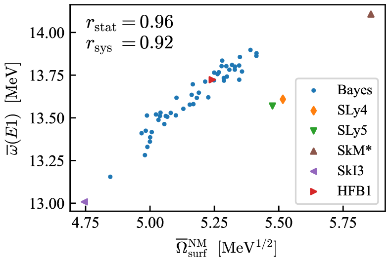
Figure 3: Correlation between the nuclear-surface isovector oscillating frequency $\overline{\Omega}^{\rm NM}_{\rm surf}$ (29) and the average $E1$ peak position $\overline{\omega}(E1)$ (28), obtained from FAM calculations with different Skyrme EDFs. The correlation coefficient (CC) of the two quantities calculated with the statistical Bayesian (Bayes) samples from the HFB1 posterior distribution is $r_{\rm stat}=0.96$, while the CC across the five EDFs that are used for the analysis of systematic uncertainties is $r_{\rm sys}=0.92$.

Figure 3 plots the value of $\overline{\omega}(E1)$ as a function of $\overline{\Omega}^{\rm NM}_{\rm surf}$ in ²⁰⁸Pb. We observe a very strong correlation between these two quantities for the statistical samples from the HFB1 posterior distribution, with a Pearson correlation coefficient of $r_{\rm stat}=0.96$. However, the correlation across functionals SLy4, SLy5, SkM*, SkI3 and HFB1 in Fig. 3 is weaker ($r_{\rm sys}=0.92$), with the points of SLy4, SLy5, and SkM* lying away from the line formed by the statistical samples. This weaker correlation suggests that other effects such as the isoscalar components of the EDF have an impact. The correlation shown in Fig. 3 demonstrates that information on $E1$ transitions can help us constrain the asymmetric (isovector) nuclear-matter properties in the Skyrme EDF. The sum rules given by FAM calculations for the (deformed) ²⁴⁰Pu nucleus give a similar correlation plot as Fig. 3.

IV.3 High-order multipole responses

Table 2 shows that the isoscalar and isovector giant quadrupole resonance (GQR) energies of ²⁰⁸Pb are close to the experimental values. In addition, the systematic uncertainty of the isoscalar GQR energy is much larger than the statistical one, while systematic and statistical uncertainties of the isovector GQR location are similar.

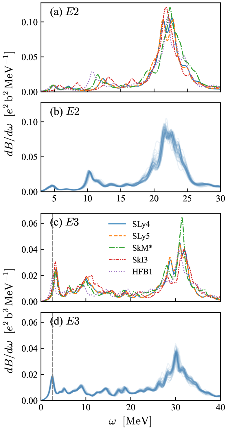
Figure 4: Panel (a): isovector electric quadrupole ($E2$) responses in ²⁰⁸Pb calculated with different Skyrme EDFs. Panel (b): similar to panel (a) but calculated with the 50 samples from the HFB1 posterior distribution. Panels (c) and (d): similar to panels (a) and (b) but for isovector electric octupole ($E3$) responses. The excitation energy of the first $3^{-}$ state of ²⁰⁸Pb [101] is marked by a dashed vertical line in panels (c) and (d). A width of $\Gamma=1$ MeV is adopted in all the panels.

Figure 4 shows the strength distributions of isovector $E2$ and $E3$ transitions in ²⁰⁸Pb; see the Supplemental Material [47] for isoscalar $E2$ and $E3$ responses in ²⁰⁸Pb. These high-order responses show features similar to the $E1$ response, with the systematic uncertainty significantly larger than the statistical one. However, we also observe multiple small peaks below the giant resonance. Some of these peaks are sensitive to the EDF choice, since they are less collective than the giant resonance and depend heavily on the s.p. structure. It is worth mentioning that the position of the lowest peak in the isovector $E3$ response is close to the first $3^{-}$ state of ²⁰⁸Pb [101], which validates the effectiveness of our calculations.

To better understand Fig. 4, we report the energy-weighted sum rules for $E2$ and $E3$ transitions in Table 4. Similar to the $E1$ transition, the values of $m_{1}(E2)$ and $m_{1}(E3)$ calculated with different Skyrme EDFs are close to each other, with SkM* being the only outlier due to its large enhancement factor $\kappa_{\rm TRK}$. This explains why the strength distributions of SkM* show higher and stronger $E2$ and $E3$ resonances.

Table 4: Energy-weighted sum rules $m_{1}$ for $E2$, $E3$, and $M1$ transitions in ²⁰⁸Pb, in the units of $e^{2}\mathrm{b}^{2}\mathrm{MeV}$, $e^{2}\mathrm{b}^{3}\mathrm{MeV}$, and $\mu_{\rm N}^{2}\cdot\mathrm{MeV}$, respectively. All the values for electric transitions are obtained from the HFB ground states calculated with various Skyrme EDFs. For the $M1$ transition, sum rules evaluated via Eq. (30) and via integrating the energy-weighted FAM strength distribution are both presented. See the caption of Table 2 for the definitions of $\bar{x}$ and $\sigma$.

	$m_{1}(E2)$	$m_{1}(E3)$	$m_{1}^{\rm SO}(M1)$	$m_{1}(M1)$
SLy4	$12.10$	$9.78$	$509.90$	$515.10$
SLy5	$12.06$	$9.72$	$519.30$	$617.50$
SkI3	$12.20$	$9.90$	$509.10$	$508.80$
SkM*	$13.84$	$10.92$	$556.50$	$563.70$
HFB1	$12.24$	$9.88$	$424.30$	$434.60$
$\bar{x}_{\rm sys}$	$12.49$	$10.04$	$503.82$	$527.94$
$\sigma_{\rm sys}$	$0.68$	$0.44$	$43.37$	$60.90$
$\bar{x}_{\rm stat}$	$12.24$	$9.88$	$432.60$	$443.90$
$\sigma_{\rm stat}$	$0.03$	$0.06$	$16.00$	$15.90$

Now we turn to the analysis of magnetic transitions. The strength distributions of isovector $M1$ and $M2$ transitions in ²⁰⁸Pb are shown in Fig. 5; see the Supplemental Material [47] for isoscalar magnetic responses in ²⁰⁸Pb. We can notice that the systematic uncertainties of magnetic transitions are much larger than those of electric transitions while the statistical uncertainties remain small. This observation is consistent with the results of Ref. [95], and agrees with the argument that predicting $M1$ giant resonances is challenging for Skyrme EDFs [102].

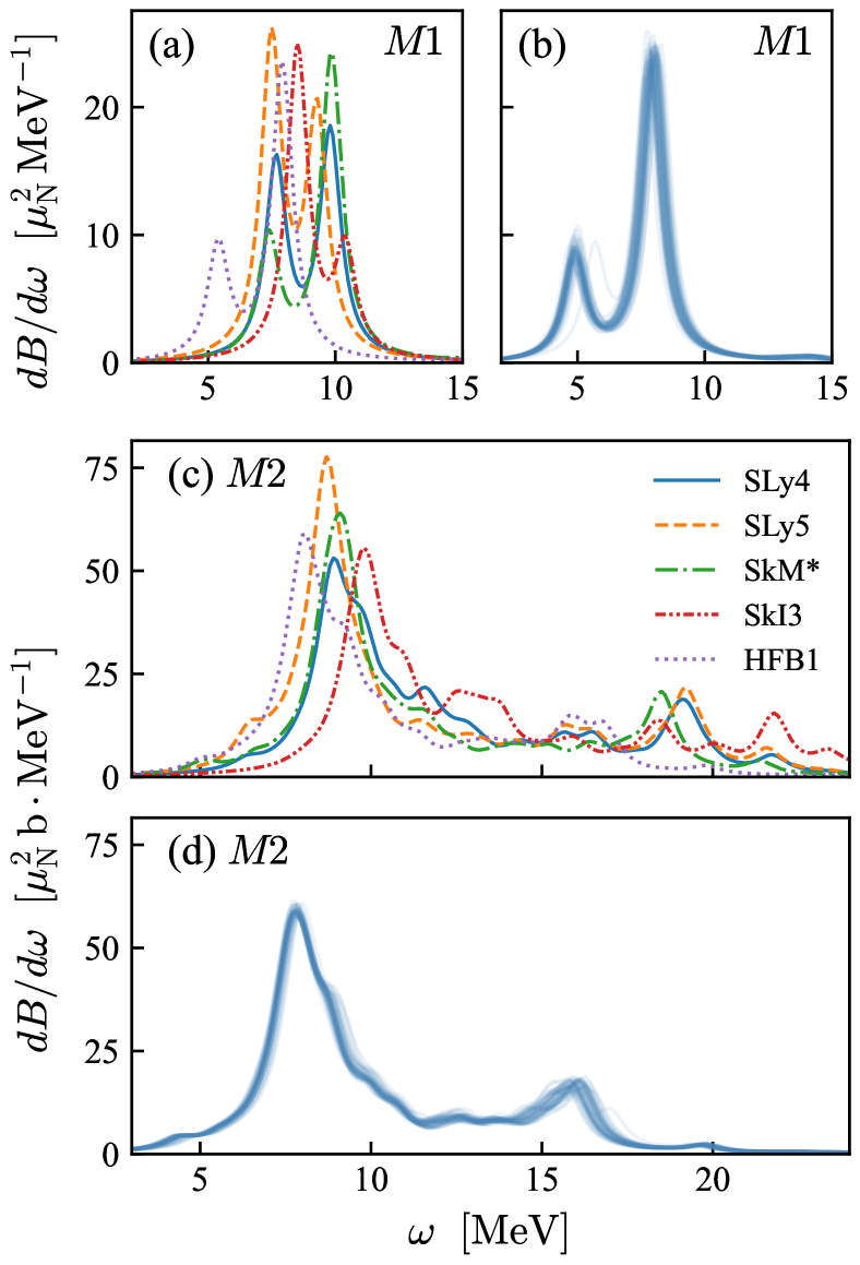
Figure 5: Similar to Fig. 4 but for isovector magnetic dipole ($M1$) and quadrupole ($M2$) responses in ²⁰⁸Pb.

Table 4 also presents the energy-weighted sum rules evaluated with the FAM response function for the $M1$ transition. We can see that $m_{1}(M1)$ has a larger systematic uncertainty than the statistical one, which is consistent with Fig. 5. In principle we can calculate $m_{1}(M1)$ via Eq. (23), but the corresponding expression is too complicated for our analysis [103]. Instead, we use the HFB spin-orbit energy $E_{\rm SO}$ to calculate the Kurath sum rule [104, 63]

$$m_{1}^{\rm SO}(M1)=-\frac{3}{16\pi}\left(g_{s}^{(n)}+g_{s}^{(p)}\right)^{2}\mu_{\rm N}^{2}E_{\rm SO},$$ (30)

which provides the largest contribution to the exact sum rule $m_{1}(M1)$, especially when the tensor term is not present. The quantity $m_{1}^{\rm SO}(M1)$ shown in Table 4 has again a large systematic but a small statistical uncertainty, in agreement with the the exact sum rule $m_{1}(M1)$. Therefore, the systematic uncertainty for the $M1$ response can be partly attributed to the uncertainty of the HFB spin-orbit energy, which is expected to be sensitive to the s.p. structure. In contrast, the electric multipole resonances are more collective and less dependent on the details of s.p. levels. Moreover, we notice in Table 4 that the inclusion of the tensor term in SLy5 significantly enlarges the difference between the Kurath and exact sum rules, making Eq. (30) a worse approximation for $m_{1}(M1)$ when the tensor term is present.

V Electromagnetic Responses in Actinide Nuclei

In this section, we review the electromagnetic response properties – either the photoabsorption cross sections or high-order responses – in actinide nuclei. These include even-even, odd-mass and odd-odd nuclei.

V.1 Odd-mass and odd-odd isotopes

In odd-$A$ and odd-odd nuclei, the HFB solution on top of which the nuclear response is computed depends on the blocking configuration(s), which sets the spin and parity of the nucleus. For most EDFs, it is not guaranteed that the lowest-energy blocking configuration gives the observed spin and parity of the nucleus. In this section, we use ²³⁹U (odd-$A$) and ²³⁸Np (odd-odd) to study the sensitivity of multipole responses to the choice of underlying blocking configurations. To eliminate uncertainties related to the parameters of the EDF, we only consider the SLy4 parameterization in the following.

V.1.1 Ground-state energies and sum rules

In hfbtho the dimensionless quadrupole deformation $\beta_{2}$ is defined as $\beta_{2}=\sqrt{\pi/5}\langle 2z^{2}-x^{2}-y^{2}\rangle/\langle r^{2}\rangle$, where $\langle\cdots\rangle$ represents the expectation value in the static HFB state. Table 5 gives the HFB energy and quadrupole deformation $\beta_{2}$ of ²³⁹U for different neutron blocked orbits. While the impact of the blocking configuration on the ground-state energy is of the order of a few hundreds of keV, the deformation of ²³⁹U does not vary much, except when we block $[770]1/2^{-}$, an intruder orbit that has a large value of $n_{z}$ and thus a density profile concentrated along the $z$ axis. The same observation can also be made for different combinations of neutron and proton blocked orbits in ²³⁸Np, where blocking the intruder neutron state $[770]1/2^{-}$ leads to a larger HFB deformation.

Table 5: HFB energies $E_{\rm HFB}$ in MeV, quadrupole deformations $\beta_{2}$, and energy-weighted sum rules $m_{1}$ for $E1$ and $E2$ ($K=0,2$) transitions in the units of $e^{2}\mathrm{b}\cdot\mathrm{MeV}$ and $e^{2}\mathrm{b}^{2}\mathrm{MeV}$, obtained with various neutron blocked orbits in ²³⁹U. We use the SLy4 parameterization and ²³⁸U as the core for blocking. Blocked orbits are labeled by their asymptotic (Nilsson) quantum numbers $[Nn_{z}\Lambda]\Omega^{\pi}$. The uncertainty $\sigma_{\rm blck.}$ is given by the standard deviation of the results obtained with different blocked orbits.

	$E_{\rm HFB}$	$\beta_{2}$	$m_{1}(E1)$	$m_{1}(E2)$
				$K=0$	$K=2$
$[622]5/2^{+}$	$\text{-}1794.72$	$0.273$	$3.3124$	$18.61$	$13.06$
$[743]7/2^{-}$	$\text{-}1794.67$	$0.268$	$3.3122$	$18.53$	$13.10$
$[624]7/2^{-}$	$\text{-}1794.37$	$0.265$	$3.3118$	$18.50$	$13.13$
$[631]1/2^{+}$	$\text{-}1793.95$	$0.263$	$3.3122$	$18.47$	$13.14$
$[770]1/2^{-}$	$\text{-}1793.76$	$0.290$	$3.3119$	$18.86$	$12.95$
$\sigma_{\rm blck.}$	$0.38$	$0.010$	$0.0002$	$0.14$	$0.07$

V.1.2 $E1$ transition

Figure 6 presents the $E1$ photoabsorption cross sections of ²³⁹U and ²³⁸Np obtained with various blocked orbits. First, we see that the uncertainty brought by the choice of blocked orbits is much smaller than the systematic uncertainty shown in Sec. IV.1. In ²³⁹U (upper panel of Fig. 6), the outlier among all the curves is given by the intruder state $[770]1/2^{-}$: the peak at $\omega=10\sim 11$ MeV, which originates from the $K=0$ component, slightly moves leftward when we block $[770]1/2^{-}$. This shift can be attributed to the larger HFB deformation brought by the intruder state, which results in a longer effective oscillator length in the $z$ direction. On the other hand, the $|K|=1$ component that gives peaks at higher energies is less impacted by the choice of the blocked orbit, indicating that the effective oscillator lengths along $x$ and $y$ axes stay stable no matter which state we block. The same conclusion can also be drawn from the cross sections of ²³⁸Np.

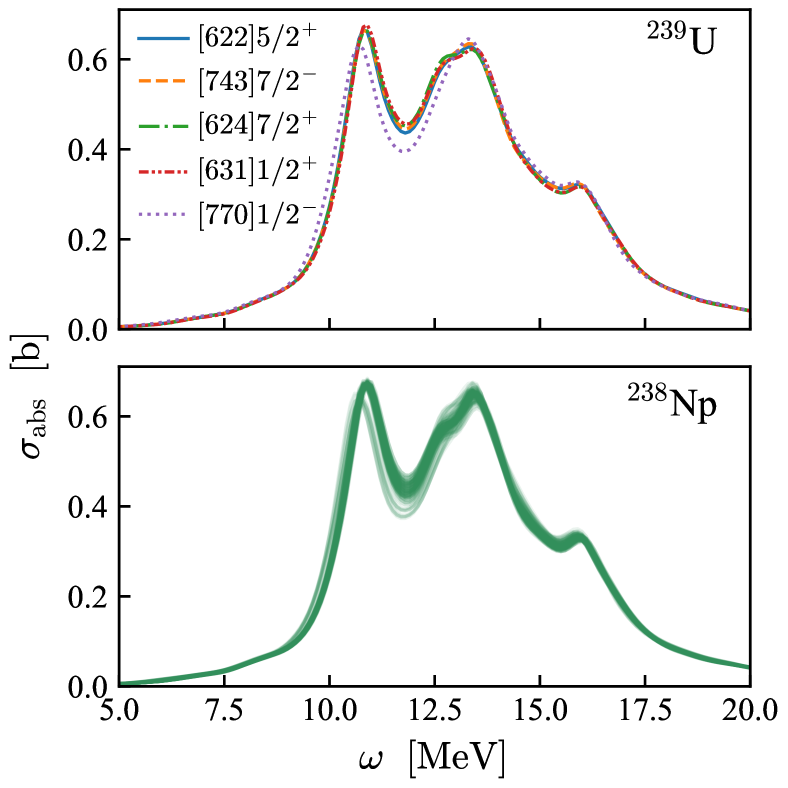
Figure 6: Photoabsorption cross sections of ²³⁹U (upper panel) and ²³⁸Np (lower panel), calculated with the SLy4 parameterization and different blocked orbits. Neutron blocked states in ²³⁹U are labeled by asymptotic quantum numbers $[Nn_{z}\Lambda]\Omega^{\pi}$. Neutron and proton blocked orbits in ²³⁸Np are given in the Supplemental Material [47]. A width of $\Gamma=1$ MeV is adopted in both panels.

The energy-weighted sum rules $m_{1}$ for the $E1$ transitions in ²³⁹U calculated with different blocked states are also given in Table 5. We notice that the sum rule $m_{1}(E1)$ has very weak dependence on the choice of the blocked orbit, indicating that the corresponding HFB solutions share similar density profiles that enter Eq. (25). This places a constraint on how much variation the cross section can have in Fig. 6.

V.1.3 $E2$ and $M1$ transitions

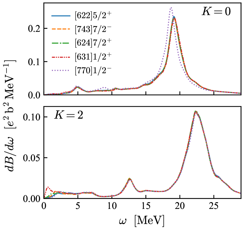
Figure 7: Similar to Fig. 6, but for $K=0$ and $K=2$ contributions to the isovector $E2$ response in ²³⁹U.

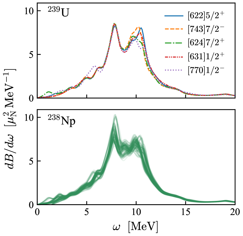
Figure 8: Similar to Fig. 6 but for the $K=0$ components of isovector $M1$ responses.

Figure 7 shows the dependency of the isovector $E2$ response on the blocking configuration. For the $K=0$ component, the $E2$ resonance is shifted to a lower energy when the intruder state $[770]1/2^{-}$ is blocked, while other blocking configurations give nearly identical responses. When the angular-momentum projection $K$ increases, the dependence on the blocking configuration becomes even weaker. The $K=2$ component shown in the lower panel of Fig. 7 hardly changes when we block different orbits, except at $\omega$ around 1 MeV. These observations also apply to the $E2$ response in ²³⁸Np, and they are consistent with what we see in Sec. V.1.2 for $E1$ transitions.

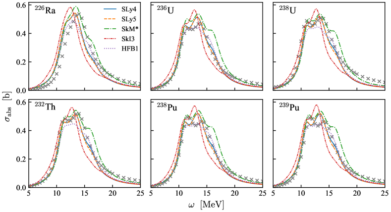
Figure 9: Photoabsorption cross sections of ²²⁶Ra, ²³²Th, ^236,238U and ^238,239Pu, calculated with different Skyrme parameterizations and a width of $\Gamma=2$ MeV. The evaluated nuclear data [91] are denoted by cross markers.

Unlike the $E1$ transition, Table 5 shows that the energy-weighted sum rules for the $E2$ transition in ²³⁹U have some dependence on the blocked orbit. The sum rule for the $K=0$ component varies significantly when the $[770]1/2^{-}$ orbit is blocked, since Eq. (52a) shows that it is sensitive to how far the nuclear density extends in the $z$ direction. This explains the stronger resonance of $[770]1/2^{-}$ in Fig. 7. The sum rule for the $K=2$ component, however, is less sensitive to blocking; according to Eq. (52c), it depends on how extended the nucleus is in $x$ and $y$ directions, which barely changes when we block different states.

Figure 8 displays the dependence of $M1$ responses ($K=0$) on the blocked states in ²³⁹U and ²³⁸Np. Overall, the magnetic response is much more sensitive to the blocking configuration. Together, Figs. 5 and 8 suggest strong dependence of $M1$ transitions on the s.p. structure. Therefore, magnetic responses have large uncertainties related to the EDF parameterization and the choice of blocked orbits.

V.2 Photoabsorption cross sections of major actinides

In this section we study the photoabsorption cross sections of major actinides and their uncertainties. With the help of monoenergetic, high-intensity $\gamma$-ray sources such as TUNL [105], fission properties of actinides can be measured with very high accuracy as functions of excitation energy in photon-induced reactions; see, e.g., [106, 107, 108] for recent examples. At the same time, radiative processes such as $(n,\gamma)$ that are essential in nuclear astrophysical simulations can be probed indirectly from photonuclear reactions $(\gamma,n)$. Such calculations begin with the determination of the total photoabsorption cross section.

Since the total uncertainty is dominated by the systematic one, as shown in Secs. IV and V.1, we only perform calculations for the five different functionals used throughout this paper. Figure 9 shows the photoabsorption cross sections of ²²⁶Ra, ²³²Th, ^236,238U and ^238,239Pu. Like Fig. 1 for ²⁰⁸Pb, FAM calculations for nuclei in Fig. 9 are performed with $\Gamma=2$ MeV for comparison with the reference database [91]. Note that ²²⁶Ra has an octupole-deformed ground state and ²³⁹Pu is an odd-mass isotope with spin 1/2⁺. Table 6 shows the quantum numbers of blocking configurations for the ground state of ²³⁹Pu calculated with different Skyrme parameterizations: only with SkM* do we obtain the proper spin-parity assignment of the ground state, yet other functionals such as SLy4, SLy5 and HFB1 better reproduce the cross section data.

Table 6: Ground-state blocked orbits in ²³⁹Pu for various Skyrme EDFs, labeled by asymptotic (Nilsson) quantum numbers $[Nn_{z}\Lambda]\Omega^{\pi}$. The even-even nucleus core is ²⁴⁰Pu.

SLy4	SLy5	SkM*	SkI3	HFB1
[7,4,3]$\tfrac{7}{2}^{-}$	[6,2,2]$\tfrac{5}{2}^{+}$	[6,3,1]$\tfrac{1}{2}^{+}$	[6,2,4]$\tfrac{7}{2}^{+}$	[7,4,3]$\tfrac{7}{2}^{-}$

Overall, we obtain good agreement between FAM predictions and reference evaluations, with the results of SkM* and SkI3 being slightly worse than other EDFs. Furthermore, the cross sections of different nuclei share similar patterns; the similarity is most pronounced when we compare the results of two U (or Pu) isotopes.

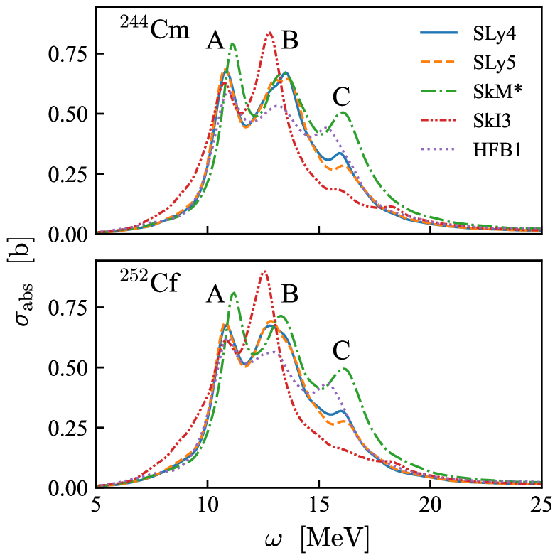
Figure 10: Photoabsorption cross sections of ²⁴⁴Cm and ²⁵²Cm calculated with different Skyrme EDFs and a width of $\Gamma=1$ MeV.

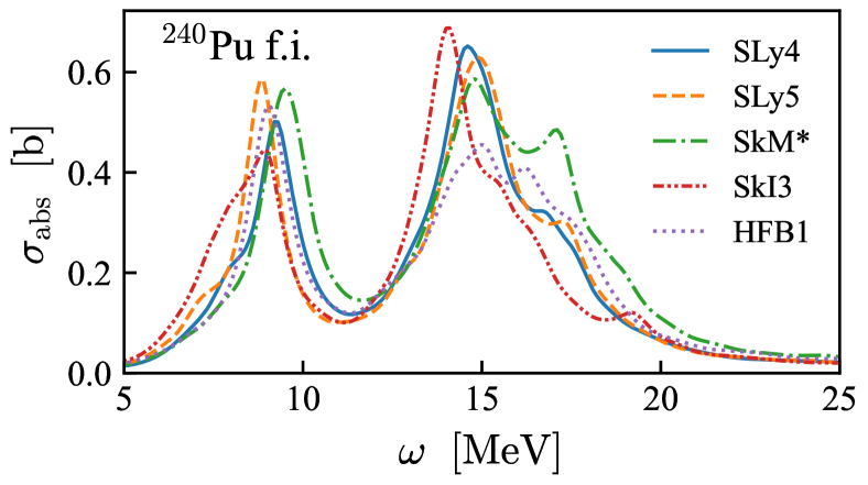
Figure 11: Similar to Fig. 10 but for the fission isomer (f.i.) of ²⁴⁰Pu.

In Figs. 10 and 11, we show the photoabsorption cross sections of ²⁴⁴Cm, ²⁵²Cf, and the fission isomer (f.i.) of ²⁴⁰Pu. For these calculations, we adopt $\Gamma=1$ MeV to better highlight individual peaks. We note that the cross sections of ²⁴⁴Cm and ²⁵²Cf have very similar patterns. In Fig. 10 peaks “B” and “C” ($|K|=1$) have larger systematic uncertainties than the peak “A” ($K=0$), which is consistent with Fig. 2 for ²⁴⁰Pu. By comparing Figs. 2 and 11, we see that the photoabsorption cross section of the ²⁴⁰Pu fission isomer is significantly different from that of the ground state. This is largely determined by the fact that the fission isomer has a much larger deformation ($\beta_{2}\approx 0.7$) than the ground state, which leads to stronger fragmentation in Fig. 11.

V.3 Multipole responses along the plutonium isotopic chain

The gfam code is an efficient tool for large-scale studies of multipole responses through the nuclear landscape. As an example of its capability, in this section we present the FAM responses in even-even plutonium isotopes from the two-proton to the two-neutron dripline. In this section, all HFB and FAM calculations were performed with the Skyrme parameterization SLy4. In this case, we find that the two-proton dripline is located at $N=122$ and the two-neutron dripline at $N=210$.

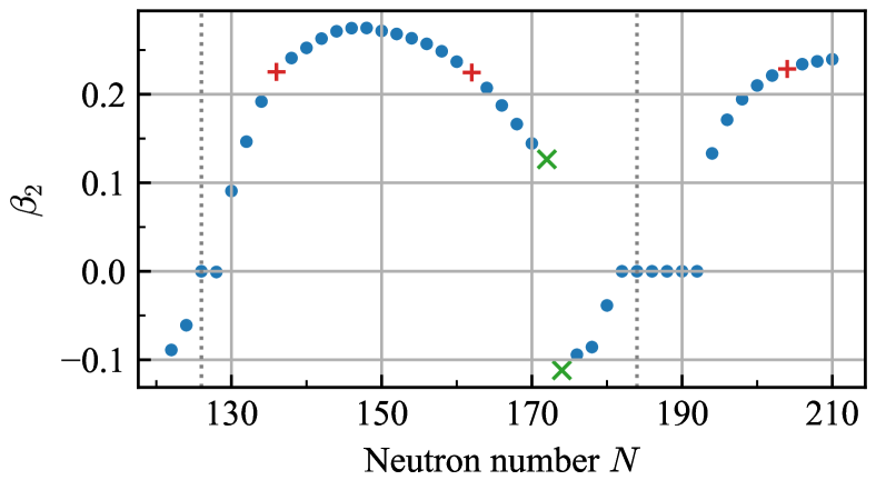
Figure 12: HFB ground-state quadrupole deformations of even-even plutonium isotopes from $N=122$ to $N=210$. Isotopes denoted by red “+” markers at $N=134$, $162$, and $204$ are shown in the right panel of Fig. 13; isotopes marked by green crosses at $N=172$ and $174$ are shown in Fig. 14. Neutron magic numbers $N=126$ and $184$ are marked by dotted vertical lines.

To better analyze the responses along the isotopic chain, we first show in Fig. 12 the HFB ground-state quadrupole deformations of these Pu isotopes. We observe two transitions from an oblate to a prolate nuclear shape, one from neutron number $N=128$ to $130$, and the other from $N=180$ to $194$. There is also a transition from a prolate to an oblate shape at $N=172\sim 174$. In the following we will discuss how these shape changes impact various multipole responses.

V.3.1 $E1$ transitions

We first present the $E1$ photoabsorption cross sections of all the even-even Pu isotopes in the left panel of Fig. 13, where we can clearly see how much the cross section varies as the neutron number $N$ changes. A detailed figure for the photoabsorption cross section of each plutonium isotope can be found in the Supplemental Material [47]. In the following we will closely examine the impact of the ground-state deformation on the $E1$ photoabsorption cross sections of Pu isotopes.

Figure 13: Panel (a): photoabsorption cross sections of even-even Pu isotopes from the two-proton to the two-neutron dripline ($N=122$ to $210$), calculated with the SLy4 parameterization and a width of $\Gamma=1$ MeV. Panel (b): similar to panel (a) but for Pu isotopes around $N=194$, showing the effect resulting from the onset of ground-state quadrupole deformation. Panel (c): similar to panel (a) but for three different well-deformed, prolate Pu isotopes with similar ground-state deformations $\beta_{2}\approx 0.23$, denoted by red plus markers in Fig. 12.

The variations of the photoabsorption cross section around $N=194$, where a spherical-prolate shape transition occurs, are displayed in the middle panel of Fig. 13. As the neutron number increases, the cross section barely changes before the shape transition, but then the onset of quadrupole deformation significantly alters the cross section and makes it more fragmented, as the degeneracy on the angular-momentum projection of the external field is broken in a deformed nucleus. After the shape transition the cross section gradually becomes stabilized as the deformation $\beta_{2}$ also stabilizes.

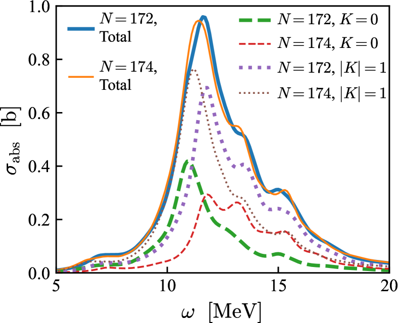
Figure 14: Photoabsorption cross sections of ^266,268Pu, as well as their $K=0$ and $|K|=1$ components, calculated with the SLy4 parameterization and a width of $\Gamma=1$ MeV.

Besides the shape transitions from an oblate to a prolate shape, we also notice a prolate-oblate shape transition from $N=172$ to $174$ in Fig. 12. As shown in Fig. 14, this shape transition barely influences the total photoabsorption cross section, which is quite different from the spherical-prolate transition shown in Fig. 13. By decomposing the total cross section into $K=0$ and $|K|=1$ components, we can see in Fig. 14 that the two components change dramatically when the shape transition occurs, but their variations roughly compensate each other. When the prolate-oblate transition occurs, the nucleus shrinks in the $z$ direction but becomes more extended in $x$ and $y$ directions. Therefore, the effective $E1$ oscillators along the $z$ axis and in the perpendicular direction are basically swapped during the prolate-oblate transition, which leads to an almost unchanged total cross section.

In order to better inspect the isotopic dependence, we show in the right panel of Fig. 13 the photoabsorption cross sections of three Pu isotopes with similar deformations $\beta_{2}\approx 0.23$ but different neutron numbers. We find that their cross sections have similar patterns, which can be attributed to their similar shapes. On the other hand, the cross-section curve in the right panel of Fig. 13 shifts toward a lower energy as the neutron number increases, since the effective $E1$ oscillator length increases with the nuclear radius when the neutron number grows.

V.3.2 High-order multipole responses

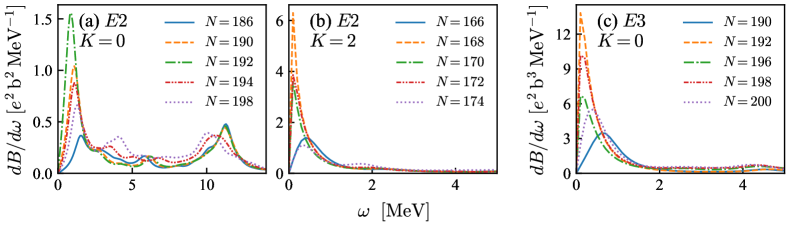
Figure 15: Panel (a): $K=0$ components of isoscalar $E2$ responses in Pu isotopes around $N=192$, showing the onset of ground-state quadrupole deformation. Panel (b): $K=2$ components of isoscalar $E2$ responses in Pu isotopes around $N=170$, showing the onset and disappearance of ground-state $\gamma$ softness. Panel (c): $K=0$ components of isoscalar $E3$ responses in Pu isotopes around $N=196$, showing the onset and disappearance of ground-state octupole softness. Responses in all the panels are calculated with the SLy4 parameterization and a width of $\Gamma=1$ MeV.

High-order responses in even-even plutonium isotopes have features similar to the $E1$ photoabsorption cross sections presented in Sec. V.3.1. Here we focus on the modes near $\omega=0$ for isoscalar $E2$ and $E3$ responses and discuss their relations with corresponding HFB ground-state multipole moments.

Figure 15 shows the low-energy responses for the isoscalar $E2$ ($K=0$ and $2$) and isoscalar $E3$ ($K=0$) transitions in Pu isotopes that exhibit strong transition strengths near $\omega=0$. We do not show the $K=1$ component of the isoscalar $E2$ response because the rotational spurious mode always gives a zero-energy peak for a deformed nucleus. For the $K=0$ component of the $E2$ response presented in the left panel of Fig. 15, the low-energy mode shifts leftward and becomes stronger as the neutron number increases to $N=192$ (before the spherical-prolate shape transition). This indicates that the quadrupole-deformed HFB minimum becomes lower in energy and closer to the energy of the spherical ground state. After the spherical-prolate shape transition, the low-energy mode becomes weaker and moves away from $\omega=0$.

For the $K=2$ component of the isoscalar $E2$ response shown in the middle panel of Fig. 15, we observe similar strong low-energy peaks around $N=170$, just before the prolate-oblate shape transition. For these Pu isotopes, the energy of their HFB prolate and oblate minima are getting closer to each other as the neutron number increases to $N=174$. We thus expect that these isotopes are $\gamma$-soft and probably have triaxial-deformed ground states, which results in the zero-energy modes seen in the middle panel of Fig. 15.

To verify this, we perform constrained $(Q_{20},Q_{22})$ HFB calculations with the triaxial code hfodd [109] for the isotopes of $N=166\sim 174$. The resulting potential energy surfaces (PESs) are shown in the Supplemental Material [47]. We find that the PES for $N=166$ shows a well-pronounced axial minimum, which becomes weakly triaxial as the neutron number rises to $N=172$. Then the PES for $N=174$ exhibits prolate-oblate shape coexistence, i.e., the energies of prolate and oblate minima are very close to one another.

The same phenomenon can also be observed in the right panel of Fig. 15 for the isoscalar $E3$ response around $N=196$. This $E3$ zero-energy peak occurs just around the spherical-prolate shape transition, where Pu isotopes are known to be octupole-soft and can have pear-shaped ground state [110]. In summary, Fig. 15 demonstrates that low-energy FAM responses can be good diagnostic tools for ground-state multipole deformations and PES softness that may not be probed by the HFB solver. Conversely, it also shows that an accurate FAM descriptions of low-energy responses demand that we find the true HFB minimum.

VI Conclusions

In this article, we developed an efficient FAM code to perform large-scale calculations for electromagnetic multipole responses in even-even, odd-$A$ and odd-odd heavy, deformed nuclei. We performed a careful analysis of the uncertainties of multipole responses induced by the parametrization of the Skyrme EDF, the calibration of the EDF (=statistical), and different configurations available for blocking in odd-mass and odd-odd nuclei.

We find that the calculated photoabsorption cross sections of fissioning nuclei with standard Skyrme functionals are in good agreement with the reference database [91]. In both spherical and deformed nuclei, the difference in the linear response between different parameterizations of the Skyrme EDF (systematic uncertainty) is much larger than the statistical uncertainty propagated from the Bayesian posterior distribution of Skyrme parameters (at least in the case of HFB1), which can be partly captured by the sum rule. Furthermore, in odd-mass and odd-odd nuclei the uncertainty of the response caused by different choices of blocking configurations is minor when compared with the systematic uncertainty. Importantly, even when the systematic uncertainty is relatively large, the overall structure of the multipole response is not impacted too much by the EDF parameterization. We confirm that information from electromagnetic responses could greatly help constrain isovector nuclear-matter properties in future Skyrme-EDF fits.

As the first step toward global studies of electromagnetic transitions through the nuclear landscape, we calculated the multipole responses in even-even Pu isotopes from the proton to the neutron dripline. As the neutron number increases, the response varies dramatically when a transition from an oblate to a prolate ground-state shape happens, and it changes slowly after the transition as the nuclear shape stabilizes. An exception to this relation between the ground-state deformation and response occurs during the prolate-oblate shape transition, where the total photoabsorption cross section stays stable while the ground-state shape abruptly jumps from a prolate to an oblate minima. This can be understood by the swap of effective oscillator lengths along and perpendicular to the $z$ axis in the intrinsic frame, causing cancellation between the variations of different $K$ components.

The infrastructure developed in this paper together with the clarifications of the formalism and the analysis of uncertainties is the first step toward large-scale calculations for nuclear responses over the entire chart of isotopes, which can provide crucial information for reaction and fission models as well as astrophysical studies.

Appendix A Properties of FAM amplitudes

We rewrite Eqs. (8) and (9) as

$$\begin{pmatrix}\beta(t)\\ \beta^{\dagger}(t)\end{pmatrix}=\mathbb{C}(t)\mathbb{W}(t)\begin{pmatrix}\beta\\ \beta^{\dagger}\end{pmatrix},$$ (31)

where

$$\mathbb{C}_{\mu\nu}(t)=\begin{pmatrix}e^{iE_{\mu}t}\delta_{\mu\nu}&0\\ 0&e^{-iE_{\mu}t}\delta_{\mu\nu},\end{pmatrix}$$ (32)

and

$$\mathbb{W}(t)=\mathbbm{1}+\eta\delta\mathbb{W}^{(+)}(\omega)e^{-i\omega t}+\eta\delta\mathbb{W}^{(-)}(\omega)e^{i\omega t},$$ (33)

where

$$\delta\mathbb{W}^{(+)}(\omega) =\begin{pmatrix}P(\omega)&X^{T}(\omega)\\ Y^{T}(\omega)&Q(\omega)\end{pmatrix},$$ (34a)

$$\delta\mathbb{W}^{(-)}(\omega) =\begin{pmatrix}Q^{*}(\omega)&Y^{\dagger}(\omega)\\ X^{\dagger}(\omega)&P^{*}(\omega)\end{pmatrix}.$$ (34b)

The transformation matrix $\mathbb{C}(t)\mathbb{W}(t)$ in Eq. (31) must be unitary, which means $\mathbb{W}(t)$ is unitary, i.e.,

$$\mathbb{W}^{\dagger}(t)\mathbb{W}(t)=\mathbbm{1}.$$ (35)

We thus need

$$\delta\mathbb{W}^{(+)\dagger}(\omega)+\delta\mathbb{W}^{(-)}(\omega)=0$$ (36)

to ensure the unitarity of $\mathbb{W}(t)$ up to the first order of $\eta$. This yields

$$X=-X^{T},\ Y=-Y^{T},\ Q=-P^{T}.$$ (37)

Appendix B Induced FAM quantities and pairing cutoff

To calculate the induced densities and mean fields in the FAM, we first write the time-dependent quasiparticle operator $\beta_{\mu}(t)$ in the s.p. basis:

$$\beta_{\mu}(t)=\sum_{k}\left[U^{*}_{k\mu}(t)c_{k}+V^{*}_{k\mu}(t)c^{\dagger}_{k}\right]e^{iE_{\mu}t}.$$ (38)

with

$$U(t) =U+\eta\delta U^{(+)}(\omega)e^{-i\omega t}+\eta\delta U^{(-)}(\omega)e^{i\omega t},$$ (39a)

$$V(t) =V+\eta\delta V^{(+)}(\omega)e^{-i\omega t}+\eta\delta V^{(-)}(\omega)e^{i\omega t},$$ (39b)

where $U$ and $V$ define the static Bogoliubov transformation

$$\beta_{\mu}=\sum_{k}\left[U^{*}_{k\mu}c_{k}+V^{*}_{k\mu}c^{\dagger}_{k}\right].$$ (40)

Based on Eqs. (8) and (9), we can express $\delta U^{(\pm)}(t)$ and $\delta V^{(\pm)}(t)$ in terms of FAM amplitudes:

$$\delta U_{k\mu}^{(+)}(\omega) =\Big{[}UQ^{T}(\omega)+V^{*}Y(\omega)\Big{]}_{k\mu},$$ (41a)

$$\delta U_{k\mu}^{(-)}(\omega) =\Big{[}UP^{\dagger}(\omega)+V^{*}X^{*}(\omega)\Big{]}_{k\mu},$$ (41b)

$$\delta V_{k\mu}^{(+)}(\omega) =\Big{[}VQ^{T}(\omega)+U^{*}Y(\omega)\Big{]}_{k\mu},$$ (41c)

$$\delta V_{k\mu}^{(-)}(\omega) =\Big{[}VP^{\dagger}(\omega)+U^{*}X^{*}(\omega)\Big{]}_{k\mu}.$$ (41d)

With the help of time-dependent quasiparticle spinors $U(t)$ and $V(t)$, we can obtain the time-dependent density matrix and pairing tensor as [111]

$$\rho_{kl}(t) =\sum_{\mu}\Big{[}f_{\mu}U_{k\mu}(t)U^{*}_{l\mu}(t)+g_{\mu}V^{*}_{k\mu}(t)V_{l\mu}(t)\Big{]},$$ (42a)

$$\kappa_{kl}(t) =\sum_{\mu}\Big{[}f_{\mu}U_{k\mu}(t)V^{*}_{l\mu}(t)+g_{\mu}V^{*}_{k\mu}(t)U_{l\mu}(t)\Big{]},$$ (42b)

where

$$g_{\mu}=1-f_{\mu}.$$ (43)

Besides, $\rho(t)$ and $\kappa(t)$ oscillate in the same manner as the external field $F(t)$ in Eq. (5):

$$\rho(t) =\rho_{0}+\eta\Big{[}\delta\rho(\omega)e^{-i\omega t}+\delta\rho^{\dagger}(\omega)e^{i\omega t}\Big{]},$$ (44a)

$$\kappa(t) =\kappa_{0}+\eta\Big{[}\delta\kappa^{(+)}(\omega)e^{-i\omega t}+\delta\kappa^{(-)}(\omega)e^{i\omega t}\Big{]}.$$ (44b)

Substituting Eqs. (39), (41), (42) into (44) and keeping terms linear in $\eta$, we can obtain the induced density matrix and pairing tensor:

$$\delta\rho_{kl}(\omega) =\sum_{\mu\nu}\Big{[}\left(f_{\mu}-f_{\nu}\right)U_{k\mu}P_{\mu\nu}U^{*}_{l\nu}+\left(g_{\mu}-g_{\nu}\right)V^{*}_{k\mu}Q_{\mu\nu}V_{l\nu}+\left(g_{\nu}-f_{\mu}\right)U_{k\mu}X_{\mu\nu}V_{l\nu}-\left(g_{\mu}-f_{\nu}\right)V^{*}_{k\mu}Y_{\mu\nu}U^{*}_{l\nu}\Big{]},$$ (45a)

$$\delta\kappa^{(+)}_{kl}(\omega) =\sum_{\mu\nu}\Big{[}\left(f_{\mu}-f_{\nu}\right)U_{k\mu}P_{\mu\nu}V^{*}_{l\nu}+\left(g_{\mu}-g_{\nu}\right)V^{*}_{k\mu}Q_{\mu\nu}U_{l\nu}+\left(g_{\nu}-f_{\mu}\right)U_{k\mu}X_{\mu\nu}U_{l\nu}-\left(g_{\mu}-f_{\nu}\right)V^{*}_{k\mu}Y_{\mu\nu}V^{*}_{l\nu}\Big{]},$$ (45b)

$$\delta\kappa^{(-)}_{kl}(\omega) =\sum_{\mu\nu}\Big{[}\left(f_{\mu}-f_{\nu}\right)V^{*}_{l\mu}P^{*}_{\mu\nu}U_{k\nu}+\left(g_{\mu}-g_{\nu}\right)U_{l\mu}Q^{*}_{\mu\nu}V^{*}_{k\nu}+\left(g_{\nu}-f_{\mu}\right)V^{*}_{l\mu}X^{*}_{\mu\nu}V^{*}_{k\nu}-\left(g_{\mu}-f_{\nu}\right)U_{l\mu}Y^{*}_{\mu\nu}U_{k\nu}\Big{]}.$$ (45c)

With the help of Eqs. (37) and (43), one can show that $\delta\kappa^{(\pm)}(\omega)$ is antisymmetric while $\delta\rho(\omega)$ is not necessarily Hermitian.

In an even-even nucleus at zero temperature, we have $f_{\mu}=0$ and $g_{\mu}=1$, so the amplitudes $P$ and $Q$ do not contribute in Eq. (45). In this case, we can thus exclude $P$ in the FAM equations (11a), which leads to the formalism given in Ref. [39]. With the expressions of $\delta\rho$ and $\delta\kappa^{(\pm)}$, one can then compute the induced mean field $\delta H$ using equations presented in [39]. All the matrices involved in the FAM calculation have a dimension of $N_{2\mathrm{qp}}$; they are much smaller than the QRPA matrix and can thus be efficiently constructed.

In this work we adopt a zero-range pairing force, which is known to cause divergence as the model space increases [55, 56, 57]. In static HFB calculations, the divergence can be mitigated by introducing a quasiparticle cutoff, i.e., all the quasiparticles with energies above a given threshold $E_{\rm cut}$ are discarded in the calculations of densities. In the FAM we utilize a similar cutoff recipe [74]: the summations in Eq. (42) only run over quasiparticle indices $\mu$ within the pairing window of the static HFB solution, which is equivalent to replacing $f_{\mu}$ and $g_{\mu}$ in Eq. (45) with

$$\xi_{\mu}^{\rm cut}=\begin{cases}\xi_{\mu}&E_{\mu}<E_{\rm cut}\\ 0&\text{otherwise}\end{cases},\text{ for }\xi=f\text{ or }g.$$ (46)

One negative consequence of this cutoff method is that the amplitude $Q$ now contributes to the induced densities (45) in an even-even nucleus, because $g_{\mu}-g_{\nu}\neq 0$ when $\mu$ is inside the pairing window while $\nu$ is outside. To avoid this issue we force $g_{\mu}-g_{\nu}=f_{\nu}-f_{\mu}$ in our calculations. Furthermore, the pairing cutoff breaks the antisymmetry of the induced pairing tensor $\delta\kappa^{(\pm)}$ since Eq. (43), which is employed to prove the antisymmetry, is not consistent with the cutoff (46). These inconsistencies can be removed by implementing the renormalization of the pairing force [55] or by using finite-range pairing forces.

Appendix C Energy-weighted sum rules for electric multipole transitions

In this appendix we follow the procedure presented in Ref. [63] to evaluate Eq. (23) for the Skyrme EDF. For the electric multipole operator $Q_{LK}$ (15), we have

$$m_{1}^{T}(Q)=\frac{e^{2}\hbar^{2}}{2m}\int|\bm{\nabla}f(\bm{r})|^{2}\!\left[q_{n}^{2}\rho_{n}(\bm{r})\!+\!q_{p}^{2}\rho_{p}(\bm{r})\right]d\bm{r},$$ (47)

where $f(\bm{r})=r^{L}Y_{LK}(\Omega)$. Assuming a gauge-invariant Skyrme EDF, we can write the enhancement factor $\kappa(Q)$ as

$$\kappa(Q)=\frac{e^{2}\!\left(q_{n}-q_{p}\right)^{2}\!\left(C^{\tau}_{0}-C^{\tau}_{1}\right)}{m_{1}^{T}(Q)}\int|\bm{\nabla}f|^{2}\rho_{n}(\bm{r})\rho_{p}(\bm{r})d\bm{r},$$ (48)

where $C^{\tau}_{t}$ is the coupling constant of the term $\rho_{t}\tau_{t}$ in the Skyrme EDF.

Using standard formulas for the gradient of spherical harmonics in a spherical tensor basis [61], we find

$$\left(\bm{\nabla}f\right)\cdot\bm{e}_{\mu}= (-1)^{L+K}\sqrt{L}(2L+1)\begin{pmatrix}L\!-\!1&1&L\\ K\!-\!\mu&\mu&-\!K\end{pmatrix}$$ (49)

$$\times r^{L-1}Y_{L-1,K-\mu}(\Omega),\quad\mu=0,\pm 1,$$

which involves the 3$j$ symbol $\begin{pmatrix}j_{1}&j_{2}&j_{3}\\ m_{1}&m_{2}&m_{3}\end{pmatrix}$. Then we can write $\left|\bm{\nabla}f\right|^{2}$ as

$$\left|\bm{\nabla}f(\bm{r})\right|^{2}=r^{2L-2}\sum_{J=0,2,\cdots}^{2L-2}\mathcal{C}_{LK}^{(J)}Y_{J0}(\Omega),$$ (50)

where

$$\mathcal{C}_{LK}^{(J)} =L(2L+1)^{2}(2L-1)\sqrt{\frac{2J+1}{4\pi}}\begin{pmatrix}L\!-\!1&L\!-\!1&J\\ 0&0&0\end{pmatrix}$$ (51)

$$\times\sum_{\mu=-1}^{1}(-1)^{M}\begin{pmatrix}L\!-\!1&1&L\\ M&\mu&-\!K\end{pmatrix}^{2}\begin{pmatrix}L\!-\!1&L\!-\!1&J\\ -M&M&0\end{pmatrix},$$

where $M=K-\mu$, and the first and third 3$j$ coefficients come from the product of $Y_{L-1,K-\mu}^{*}$ and $Y_{L-1,K-\mu}$ [61]. One can see that $\left|\bm{\nabla}f\right|^{2}$ always has even parity, so the sum over $J$ in (50) involves only even numbers. For example, we give below the explicit expression of $\left|\bm{\nabla}f(\bm{r})\right|^{2}$ for the $E2$ transition:

$$\Big{|}\bm{\nabla}\left[r^{2}Y_{20}(\Omega)\right]\Big{|}^{2} =\sqrt{\frac{5}{\pi}}r^{2}\left[\sqrt{5}Y_{00}(\Omega)+Y_{20}(\Omega)\right]$$ (52a)

$$=\frac{5}{4\pi}\left(4z^{2}+x^{2}+y^{2}\right),$$

$$\Big{|}\bm{\nabla}\left[r^{2}Y_{21}(\Omega)\right]\Big{|}^{2} =\frac{1}{2}\sqrt{\frac{5}{\pi}}r^{2}\left[2\sqrt{5}Y_{00}(\Omega)+Y_{20}(\Omega)\right]$$ (52b)

$$=\frac{15}{8\pi}\left(2z^{2}+x^{2}+y^{2}\right),$$

$$\Big{|}\bm{\nabla}\left[r^{2}Y_{22}(\Omega)\right]\Big{|}^{2} =\sqrt{\frac{5}{\pi}}r^{2}\left[\sqrt{5}Y_{00}(\Omega)-Y_{20}(\Omega)\right]$$ (52c)

$$=\frac{15}{4\pi}\left(x^{2}+y^{2}\right).$$

where Eq. (52a) agrees with the expression derived in Ref. [44]. With Eq. (50), the energy-weighted sum rule (47) for the electric multipole operator $Q_{LK}$ can be expressed as a function of the radial moment $\langle r^{2L-2}\rangle$ and multipole deformations $\beta_{2}$, $\beta_{4}$, …, $\beta_{2L-2}$ of the HFB ground state [44]. Therefore, constraining the EDF parameters with measurements on high-order radial moments is expected to improve the calculations of electric multipole responses [112].