Robust Score-Based Quickest Change Detection

Abstract

Methods in the field of quickest change detection rapidly detect in real-time a change in the data-generating distribution of an online data stream. Existing methods have been able to detect this change point when the densities of the pre- and post-change distributions are known. Recent work has extended these results to the case where the pre- and post-change distributions are known only by their score functions. This work considers the case where the pre- and post-change score functions are known only to correspond to distributions in two disjoint sets. This work employs a pair of “least-favorable” distributions to robustify the existing score-based quickest change detection algorithm, the properties of which are studied. This paper calculates the least-favorable distributions for specific model classes and provides methods of estimating the least-favorable distributions for common constructions. Simulation results are provided demonstrating the performance of our robust change detection algorithm.

I Introduction

In the fields of sensor networks, cyber-physical systems, biology, and neuroscience, the statistical properties of online data streams can suddenly change in response to some application-specific event ([1, 2, 3, 4]). The field of quickest change detection aims to detect the change in the underlying distribution of this observed stochastic process as rapidly as possible and in real-time – but to do so with minimal risk of detecting a change before it actually occurs. When the pre- and post-change probability density functions of the data are known, three important algorithms in the literature are the Shiryaev algorithm ([5, 6]), the cumulative sum (CUSUM) algorithm ([7, 8, 9, 10]), and the Shiryaev-Roberts algorithm ([11, 12]). These three tests calculate a sequence of statistics using the likelihood ratio of the observations and detection occurs when the statistics exceed a threshold (see [5, 6, 7, 8, 9, 11]).

The main challenge in implementing a change detection algorithm in practice is that the pre- and post-change distributions are often not precisely known. This challenge is amplified when the data is high-dimensional. Specifically, in several machine learning applications, the data models may not lend themselves to explicit distributions. For example, energy-based models ([13]) capture dependencies between observed and latent variables based on their associated energy (an unnormalized probability), and score-based deep generative models [14] generate high-quality images by learning the score function (the gradient of the log density function). These models can be computationally cumbersome to normalize as probabilistic density functions. Thus, optimal algorithms from the change detection literature, which are likelihood ratio-based tests, are computationally expensive to implement.

This issue is partially addressed in [15] where the authors have proposed the SCUSUM algorithm, a Hyvärinen score-based ([16]) modification of the CUSUM algorithm for quickest change detection. It is shown in [15] that the SCUSUM algorithm is consistent and the authors also provide expressions for the average detection delay and the mean time to a false alarm. The Hyvärinen score is invariant to scale and hence can be applied to unnormalized models. This makes the SCUSUM algorithm highly efficient as compared to the classical CUSUM algorithm for high-dimensional models.

The main limitation of the SCUSUM algorithm is that its effectiveness is contingent on knowing the precise pre- and post-change unnormalized models, i.e., knowing the pre- and post-change models within a normalizing constant. In practice, due to a limited amount of training data, the models can only be learned within an uncertainty class. To detect the change effectively, an algorithm must be robust against these modeling uncertainties. The SCUSUM algorithm is not robust in this sense. Specifically, if not carefully designed, the SCUSUM algorithm can fail to detect several (in fact, infinitely many) post-change scenarios.

As one concrete example, consider a device that monitors patient health in a hospital setting. The device observes a time series of biomedical data (e.g. patient heart rate) and detects when a patient changes from stable to unstable health condition. While it is possible to learn general patterns between patient stability and heart rate, it is also true that every patient has a unique resting heart rate. An SCUSUM algorithm trained on stable and unstable patient data will suffer premature false alarms or significant detection delays when it operates on a patient with an unusual resting heart rate due to this lack of robustness.

In this paper, a robust score-based variant of the CUSUM algorithm, called RSCUSUM, is proposed for the problem of quickest change detection. Under the assumption that the pre- and post-change uncertainty classes are disjoint and convex, we show that the algorithm is robust, i.e., can consistently detect changes for every possible post-change model. This consistency is achieved by designing the RSCUSUM algorithm using the least favorable distributions from the pre- and post-change uncertainty classes.

The problem of optimal robust quickest change detection is studied in [17]. In a minimax setting, the optimal algorithm is the CUSUM algorithm designed using the least favorable distribution. The robust CUSUM test in [17] may suffer from two drawbacks: 1) It is a likelihood ratio-based test and hence may not be amenable to implementation in high-dimensional models. 2) The notion of least favorable distribution is defined using stochastic boundedness ([17]), which may be difficult to verify for high-dimensional data.

In contrast with the work in [17], we define the notion of least favorable distribution using Fisher divergence and provide a method to effectively identify the least favorable distribution for the post-change model.

We now summarize our contributions in this paper.

1. We propose a new robust score-based quickest change detection algorithm that can be applied to score-based models and unnormalized models, namely, statistical models whose density involves an unknown normalizing constant. Specifically, we use the Hyvärinen score ([16]) to propose a robust score-based variant of the SCUSUM algorithm from [15] which we refer to as RSCUSUM. In this variant and its subsequent theory, the role of Kullback-Leibler divergence in classical change detection is replaced with the Fisher divergence between the pre-and post-change distributions. This algorithm is introduced in Section V.

2. Our generalized RSCUSUM algorithm can address unknown pre- and post-change models. Specifically, assuming that the pre- and post-change laws belong to known families of distributions which are convex, we identify a least favorable pair of distributions which are nearest in terms of Fisher divergence. We then show that the RSCUSUM algorithm can consistently detect each post-change distribution from each pre-change distribution from the relevant families, and is robust in this sense. This analysis is provided in Section VI.

3. We provide an effective method to identify the least favorable post-change distribution among pre- and post-change families. This is in contrast to the setup in [17] where a stochastic boundedness characterization makes it harder to identify the least favorable distribution. This result is presented in Section VII.

4. From a theoretical perspective, unlike the CUSUM algorithm that leverages the fact that the likelihood ratios form a martingale under the pre-change model [9, 18], the RSCUSUM algorithm is a score-based algorithm where cumulative scores do not enjoy a standard martingale characterization. Our analysis of the delay and false alarm analysis for RSCUSUM is based on new analysis techniques. This analysis is presented in Section VI.

5. We identify the least-favorable distribution for a specific case involving Gaussian mixture models. We then demonstrate the effectiveness of the RSCUSUM algorithm through simulation studies on a Gaussian mixture model and a Gauss-Bernoulli Restricted Boltzmann Machine ([19]). The identification of the least-favorable distributions for this model class is presented in Section VII with simulation results presented in Section VIII.

The remainder of this paper is organized as follows: in Section II, the problem of change-point detection is formally defined. In Section III, we review a detection algorithm in the case where the densities of the pre- and post-change distributions are known. In Section IV, we review an algorithm that detects change points when we have knowledge of the scores of the pre- and post-change distributions without knowledge of their densities.

II Problem Formulation

Let $\{X_{n}\}_{n\geq 1}$ denote a sequence of independent random variables defined on the probability space $(\Omega,\mathcal{F},\mu_{\nu})$. Let $\mathcal{F}_{n}$ be the $\sigma-$algebra generated by random variables $X_{1},\;X_{2},\;\dots,\;X_{n}$, and let $\mathcal{F}=\sigma(\cup_{n\geq 1}\mathcal{F}_{n})$ be the $\sigma-$algebra generated by the union of sub-$\sigma$-algebras $\{\mathcal{F}_{n}$}. Under $\mu_{\nu}$, $X_{1},\;X_{2},\;\dots,\;X_{\nu-1}$ are independent and identically distributed (i.i.d.) according to probability measure $P_{\infty}$ (with density $p_{\infty}$) and $X_{\nu},\;X_{\nu+1},\;\dots$ are i.i.d. according to probability measure $P_{1}$ (with density $p_{1}$). We think of $\nu$ as the change-point, $p_{\infty}$ as the pre-change density, and $p_{1}$ as the post-change density. We use $\mathbb{E}_{\nu}$ and $\text{Var}_{\nu}$ to denote the expectation and the variance associated with the measure $\mu_{\nu}$, respectively. Thus, $\nu$ is seen as an unknown constant and we have an entire family $\{\mu_{\nu}\}_{1\leq\nu\leq\infty}$ of change-point models, one for each possible change-point. We use $\mu_{\infty}$ to denote the measure under which there is no change, with $\mathbb{E}_{\infty}$ denoting the corresponding expectation.

A change detection algorithm is a stopping time $T$ with respect to the data stream $\{X_{n}\}_{n\geq 1}$:

$$\{T\leq n\}\in\mathcal{F}_{n},\quad\forall n\geq 1.$$

If $T\geq\nu$, we have made a delayed detection; otherwise, a false alarm has happened. Our goal is to find a stopping time $T$ to optimize the trade-off between well-defined metrics on delay and false alarm. We consider two minimax problem formulations to find the best stopping rule.

To measure the detection performance of a stopping rule, we use the following minimax metric ([7]), the worst-case averaged detection delay (WADD):

$$\mathcal{L}_{\texttt{WADD}}(T)\overset{\Delta}{=}\sup_{\nu\geq 1}\text{ess}\sup\mathbb{E}_{\nu}[(T-\nu+1)^{+}|\mathcal{F}_{\nu-1}],$$

where $(y)^{+}\overset{\Delta}{=}\max(y,0)$ for any $y\in\mathbb{R}$. Here $\text{ess}\sup$ is the essential supremum, i.e., the supremum outside a set of measure zero. We also consider the version of minimax metric introduced in [11], the worst conditional averaged detection delay (CADD):

$$\mathcal{L}_{\texttt{CADD}}(T)\overset{\Delta}{=}\sup_{\nu\geq 1}\mathbb{E}_{\nu}[T-\nu|T\geq\nu].$$

For false alarms, we consider the average running length (ARL), which is defined as the mean time to false alarm:

$$\text{ARL}\overset{\Delta}{=}\mathbb{E}_{\infty}[T].$$

We assume that pre- and post-change distributions are not precisely known. However, each is known within an uncertainty class. Let $\mathcal{G}_{\infty}$ and $\mathcal{G}_{1}$ be two disjoint classes of probability measures (We will discuss precise assumptions on them below). Then, we assume that the distributions $P_{\infty}$ and $P_{1}$ satisfy

$$\begin{split}P_{\infty}&\in\mathcal{G}_{\infty}\\ P_{1}&\in\mathcal{G}_{1}.\end{split}$$ (1)

The objective is to find a stopping rule to solve the following problem:

$$\min_{T}\;\sup_{P_{\infty}\in\mathcal{G}_{\infty},P_{1}\in\mathcal{G}_{1}}\mathcal{L}_{\texttt{WADD}}(T)\;\quad\text{subject to}\;\quad\mathbb{E}_{\infty}[T]\geq\gamma,$$ (2)

where $\gamma$ is a constraint on the ARL. The delay $\mathcal{L}_{\texttt{WADD}}$ in the above problem is a function of the true pre- and post-change laws $P_{\infty},P_{1}$ and should be designated as $\mathcal{L}_{\texttt{WADD}}^{P_{\infty},P_{1}}.$ We will, however, suppress this notation and simply refer to $\mathcal{L}_{\texttt{WADD}}^{P_{\infty},P_{1}}$ by $\mathcal{L}_{\texttt{WADD}}$. Thus, the goal in this problem is to find a stopping time $T$ to minimize the worst-case detection delay, subject to a constraint $\gamma$ on $\mathbb{E}_{\infty}[T]$. We are also interested in the minimax formulation:

$$\min_{T}\;\sup_{P_{\infty}\in\mathcal{G}_{\infty},P_{1}\in\mathcal{G}_{1}}\mathcal{L}_{\texttt{CADD}}(T)\;\quad\text{subject to}\;\quad\mathbb{E}_{\infty}[T]\geq\gamma.$$ (3)

Similarly, the delay $\mathcal{L}_{\text{CADD}}$ is a function of $P_{\infty},P_{1}$, but we suppress the notation and refer to $\mathcal{L}_{\text{CADD}}^{P_{\infty},P_{1}}$ as $\mathcal{L}_{\text{CADD}}$. For an overview of the literature on quickest change detection when the densities are not precisely known, we refer the readers to [1, 4, 2, 9, 7].

III Optimal Solution Based on Likelihood Ratios

If both the pre-change and post-change families are singletons, $\mathcal{G}_{1}=\{P_{1}\},\mathcal{G}_{\infty}=\{P_{\infty}\}$, and $P_{1}\neq P_{\infty}$, then the above formulations are the classical minimax formulations from the quickest change detection literature; see [1, 3, 4]. The optimal algorithm (exactly optimal for (2) and asymptotically optimal for (3)) is the CUSUM algorithm given by

$$T_{\texttt{CUSUM}}=\inf\{n\geq 1:\Lambda(n)\geq\omega\},$$ (4)

where $\Lambda(n)$ is defined using the recursion

$$\begin{split}&\Lambda(0)=0,\\ &\Lambda(n)\overset{\Delta}{=}\biggr{(}\Lambda(n-1)+\log\frac{p_{1}(X_{n})}{p_{\infty}(X_{n})}\biggr{)}^{+},\;\quad\forall n\geq 1,\end{split}$$

which leads to a computationally convenient stopping scheme. We recall that here $p_{1}$ is the post-change density and $p_{\infty}$ is the pre-change density. In [7] and [9], the asymptotic performance of the CUSUM algorithm is also characterized. Specifically, it is shown that with $\omega=\log\gamma$,

$$\mathbb{E}_{\infty}[T_{\texttt{CUSUM}}]\geq\gamma,$$

and as $\gamma\rightarrow\infty$,

$$\mathcal{L_{\texttt{WADD}}}(T_{\texttt{CUSUM}})\sim\mathcal{L_{\texttt{CADD}}}(T_{\texttt{CUSUM}})\sim\frac{\log\gamma}{\mathbb{D}_{\texttt{KL}}(P_{1}\|P_{\infty})}.$$

Here $\mathbb{D}_{\texttt{KL}}(P_{1}\|P_{\infty})$ is the Kullback-Leibler divergence between the post-change distribution and pre-change distribution:

$$\mathbb{D}_{\texttt{KL}}(P_{1}\|P_{\infty})=\int p_{1}(x)\log\frac{p_{1}(x)}{p_{\infty}(x)}dx,$$

and the notation $g(c)\sim h(c)$ as $c\to c_{0}$ indicates that $\frac{g(c)}{h(c)}\to 1$ as $c\to c_{0}$ for any two functions $c\mapsto g(c)$ and $c\mapsto h(c)$.

If the post-change densities $p_{\infty},p_{1}$ are not known and are assumed to belong to families $\mathcal{G}_{\infty},\mathcal{G}_{1}$, then the test is designed using the least favorable distributions. Specifically, in [17], it is assumed that there are densities $\bar{p}_{\infty}\in\mathcal{G}_{\infty},\bar{p}_{1}\in\mathcal{G}_{1}$ such that for every $p_{\infty}\in\mathcal{G}_{\infty}$ and $p_{1}\in\mathcal{G}_{1}$,

$$\begin{split}\log\frac{\bar{p}_{1}(X)}{\bar{p}_{\infty}(X)}\bigg{|}_{X\sim\bar{p}_{1}}\;\;\prec\quad\;\;\log\frac{\bar{p}_{1}(X)}{\bar{p}_{\infty}(X)}\bigg{|}_{X\sim p_{1}},\end{split}$$ (5)

$$\begin{split}\log\frac{\bar{p}_{1}(X)}{\bar{p}_{\infty}(X)}\bigg{|}_{X\sim\bar{p}_{\infty}}\;\;\succ\quad\;\;\log\frac{\bar{p}_{1}(X)}{\bar{p}_{\infty}(X)}\bigg{|}_{X\sim p_{\infty}}.\end{split}$$ (6)

Here the notation $\prec$ is used to denote stochastic dominance: if $W$ and $Y$ are two random variables, then $W\prec Y$ if

$$P(Y\geq t)\geq P(W\geq t),\quad\text{for all }t\in(-\infty,\infty).$$

If such densities $\bar{p}_{\infty},\bar{p}_{1}$ exist in the pre- and post-change families, then the robust CUSUM is defined as the CUSUM test with $\bar{p}_{\infty},\bar{p}_{1}$ used as the pre- and post-change densities:

$$\begin{split}&\bar{\Lambda}(0)=0,\\ &\bar{\Lambda}(n)\overset{\Delta}{=}\biggr{(}\bar{\Lambda}(n-1)+\log\frac{\bar{p}_{1}(X_{n})}{\bar{p}_{\infty}(X_{n})}\biggr{)}^{+},\forall n\geq 1.\end{split}$$

Such a test is exactly optimal for the problem of [7] under additional assumptions on the smoothness of densities, and asymptotically optimal for the problem in [11]. We refer the reader to [17] for a more precise optimality statement.

We note that in the literature on quickest change detection, the issue of the unknown post-change model has also been addressed by using a generalized likelihood ratio (GLR) test or a mixture-based test. While these tests have strong optimality properties, they are computationally even more expensive than the robust test described above; see [7, 9, 4].

IV Quickest Change Detection in Unnormalized and Score-Based Models

The limitation of the CUSUM and the robust CUSUM algorithms is that they are based on likelihood ratios which are not always precisely known. In modern machine learning applications, two new classes of models have emerged:

1. Unnormalized statistical models: In these models, we know the distribution within a normalizing constant:

   $$\begin{split}p_{\infty}(x)=\frac{\tilde{p}_{\infty}(x)}{Z_{\infty}},\quad\text{ and }\quad p_{1}(x)=\frac{\tilde{p}_{1}(x)}{Z_{1}},\end{split}$$ (7)

   where $Z_{\infty}$ and $Z_{1}$ are normalizing constants that are hard (or even impossible) to calculate by numerical integration, especially when the dimension of $x$ is high. In some applications, the unnormalized models $\tilde{p}_{\infty}(x)$ and $\tilde{p}_{1}(x)$ are known in precise functional forms. Examples include continuous-valued Markov random fields or undirected graphical models which are used for image modeling. We refer the reader to [16, 15] for detailed discussions on unnormalized models.

2. Score-based models: Often, even $\tilde{p}_{\infty}(x)$ and $\tilde{p}_{1}(x)$ are unknown. But, it may be possible to learn the scores

   $$\nabla_{x}\log p_{\infty}(x),\quad\text{ and }\quad\nabla_{x}\log p_{1}(x),$$

   from data. Here $\nabla_{x}$ is the gradient operator. This is possible using the idea of score-matching. Specifically, these scores can be learned using a deep neural network. We refer the readers to [16, 14, 20, 21, 15, 22] for details. We note that a score-based model is also unnormalized where the exact form of the unnormalized function is hard to estimate.

In a recent work [15], the authors have developed a score-based CUSUM (SCUSUM) algorithm to detect changes in unnormalized and score-based models and also obtained its performance characteristics. In the score-based theory in [15], the Kullback-Leibler divergence is replaced by the Fisher divergence (defined precisely below) between the pre- and post-change densities.

The SCUSUM algorithm is defined based on Hyvärinen Score ([16]), which circumvents the computation of normalization constants and has found diverse applications including Bayesian model comparison [23], information theory [24], and hypothesis testing [22]. We first define the Hyvärinen Score below.

Definition IV.1 (Hyvärinen Score).

The Hyvärinen score of any probability measure $P$ (with density $p$) is a mapping $(x,P)\mapsto\mathcal{S}_{\texttt{H}}(x,P)$ given by

$$\mathcal{S}_{\texttt{H}}(x,P)\overset{\Delta}{=}\frac{1}{2}\left\|\nabla_{x}\log p(x)\right\|_{2}^{2}+\Delta_{x}\log p(x),$$

whenever it can be well defined. We assume that the Hyvärinen scores is well defined for all $P\in\mathcal{G}_{\infty}\cup\mathcal{G}_{1}$ by Assumption V.3. Here, $\|\cdot\|_{2}$ denotes the Euclidean norm, $\nabla_{x}$ and $\Delta_{x}=\sum_{i=1}^{d}\frac{\partial^{2}}{\partial x_{i}^{2}}$ respectively denote the gradient and the Laplacian operators acting on $X=(x_{1},\cdots,x_{d})^{\top}$.

By using the Hyvärinen Score in our algorithm, the role of Kullback-Leibler divergence in the theoretical analysis of the algorithm is replaced by the Fisher divergence.

Definition IV.2 (Fisher Divergence).

The Fisher divergence between two probability measures $P$ to $Q$ (with densities $p$ and $q$) is defined by

$$\mathbb{D}_{\texttt{F}}(P\|Q)\overset{\Delta}{=}\mathbb{E}_{X\sim P}\left[\left\|\nabla_{{x}}\log p(X)-\nabla_{{x}}\log q(X)\right\|_{2}^{2}\right],$$ (8)

whenever the integral is well defined.

Clearly, $\nabla_{{x}}\log p(x)$, $\nabla_{{x}}\log q(x)$, and $\Delta_{x}\log q(x)$ remain invariant if $p$ and $q$ are scaled by any positive constant with respect to $x$. Hence, the Fisher divergence and the Hyvärinen Score remain scale-variant concerning an arbitrary constant scaling of density functions.

To design the SCUSUM algorithm, the precise knowledge of probability measures $P_{\infty}$ and $P_{1}$ is not required. It is enough if we know the densities in unnormalized form or know their scores. Specifically, if we can calculate the Hyvärinen scores $\mathcal{S}_{\texttt{H}}(x,P_{\infty})$ and $\mathcal{S}_{\texttt{H}}(x,P_{1})$, then we can define the SCUSUM algorithm as

$$T_{\texttt{SCUSUM}}=\inf\{n\geq 1:Y(n)\geq\omega\},$$ (9)

where $\omega>0$ is a stopping threshold that is pre-selected to control false alarms, and $Z(n)$ can be computed recursively:

$$Y(0)=0,$$

$$Y(n)\overset{\Delta}{=}(Y(n-1)+\mathcal{S}_{\texttt{H}}(X_{n},P_{\infty})-\mathcal{S}_{\texttt{H}}(X_{n},P_{1}))^{+},\;\forall n\geq 1.$$

The following theorem is established in [15] regarding the consistency and the performance of the SCUSUM algorithm.

Theorem IV.3 ([15]).

Assume that the densities $p_{\infty}$ and $p_{1}$ satisfy the regularity conditions mentioned in Assumptions II.2 and II.3. Then the following statements are true:

1. The SCUSUM algorithm is consistent. Specifically, the drift of the statistic is negative before the change and is positive after the change:

   $$\begin{split}\mathbb{E}_{\infty}\left[\mathcal{S}_{\texttt{H}}(X_{1},P_{\infty})-\mathcal{S}_{\texttt{H}}(X_{1},P_{1})\right]\;&=\;-\mathbb{D}_{\texttt{F}}(P_{\infty}\;\|\;P_{1})<0,\\ \mathbb{E}_{1}\left[\mathcal{S}_{\texttt{H}}(X_{1},P_{\infty})-\mathcal{S}_{\texttt{H}}(X_{1},P_{1})\right]\;&=\mathbb{D}_{\texttt{F}}(P_{1}\;\|\;P_{\infty})>0.\end{split}$$ (10)

2. Let there exist a $\lambda>0$ such that

   $$\mathbb{E}_{\infty}[\exp(\lambda(\mathcal{S}_{\texttt{H}}(X_{1},P_{\infty})-\mathcal{S}_{\texttt{H}}(X_{1},P_{1})))]\leq 1.$$ (11)

   Then, for any $\omega>0$,

   $$\mathbb{E}_{\infty}[T_{\texttt{SCUSUM}}]\geq e^{\lambda\omega}.$$ (12)

   Thus, setting $\omega=\frac{\log\gamma}{\lambda}$ in (9) implies

   $$\mathbb{E}_{\infty}[T_{\texttt{SCUSUM}}]\geq\gamma.$$

   Thus, similar to the CUSUM algorithm, even the SCUSUM algorithm enjoys a universal lower bound on the mean time to false alarm for any distribution pair $(P_{\infty},P_{1})$. A $\lambda$ satisfying (11) always exists, otherwise, the problem is trivial.

3. Finally, with $\omega=\frac{\log\gamma}{\lambda}$, the delay performance is given by

   $$\mathcal{L_{\texttt{WADD}}}(T_{\texttt{SCUSUM}})\sim\frac{\log\gamma}{\lambda\mathbb{D}_{\texttt{F}}(P_{1}\;\|\;P_{\infty})},\quad\text{ as }\gamma\to\infty.$$ (13)

   Thus, the expected detection delay depends inversely on the Fisher divergence between $P_{1}$ and $P_{\infty}$. Thus, the role of KL-divergence in the classical CUSUM algorithm is replaced by the Fisher divergence in the score-based CUSUM algorithm.

V Robust Quickest Change Detection in Unnormalized and Score-Based Models

In most applications, even the scores are not precisely known. For example, not enough training data may be available for precise score-matching. Thus, the SCUSUM algorithm cannot be applied. In this paper, we take a robust approach to address this issue. Specifically, we assume that both $\mathcal{G}_{\infty}$ and $\mathcal{G}_{1}$ are families of unnormalized or score-based models. In addition, we assume that there exists a pair of least favorable distributions $Q_{\infty},Q_{1}$ in the following sense:

Definition V.1 (Least-favorable distributions (LFD)).

We say that a pair of distributions $(Q_{\infty},Q_{1})$ are least favorable if they are a solution to the following optimization problem:

$$Q_{\infty},Q_{1}=\operatorname*{arg\,min}_{R_{\infty}\in\mathcal{G}_{\infty},R_{1}\in\mathcal{G}_{1}}\mathbb{D}_{F}(R_{1}\|R_{\infty}).$$ (14)

Thus, the distributions $Q_{\infty}\in\mathcal{G}_{\infty},Q_{1}\in\mathcal{G}_{1}$ are closest as measured through the pseudo distance of Fisher divergence (see (8)). We remark that since the observations are assumed to be high-dimensional, the densities are not precisely known. As a consequence, the stochastic boundedness condition of [17] or the KL divergence cannot be used here to define the least favorable pair. On the other hand, the Fisher divergence can be computed for unnormalized and score-based models. In the rest of the paper, we assume that we can always find the least favorable pair $(Q_{\infty},Q_{1})$. In Section VII, we provide several examples where this assumption is valid.

We impose the following conditions on the classes $\mathcal{G}_{\infty}$ and $\mathcal{G}_{1}$. All lemmas and theorems in the paper, unless otherwise stated, will be assumed to be valid when all these conditions are satisfied.

Assumption V.2.

$\mathcal{G}_{\infty},\mathcal{G}_{1}$ are disjoint and are each convex.

Assumption V.3.

For each $P\in\mathcal{G}_{\infty}\cup\mathcal{G}_{1}$, mild regularity conditions introduced in [16] hold.

Assumption V.4.

All $P\in\mathcal{G}_{\infty}\cup\mathcal{G}_{1}$ share the same support $\mathcal{X}$.

We now use $Q_{\infty},Q_{1}$ and their densities $q_{\infty},q_{1}$ to design a robust score-based cumulative sum (RSCUSUM) algorithm. We define the instantaneous RSCUSUM score function $x\mapsto z(x)$ by

$$z(x)\overset{\Delta}{=}\mathcal{S}_{\texttt{H}}(x,Q_{\infty})-\mathcal{S}_{\texttt{H}}(x,Q_{1}),$$ (15)

where $\mathcal{S}_{\texttt{H}}(x,Q_{\infty})$ and $\mathcal{S}_{\texttt{H}}(x,Q_{1})$ are respectively the Hyvärinen score functions of $Q_{\infty}$ and $Q_{1}$. Our proposed stopping rule is given by

$$T_{\texttt{RSCUSUM}}=\inf\{n\geq 1:Z(n)\geq\omega\},$$ (16)

where $\omega>0$ is a stopping threshold that is pre-selected to control false alarms, and $Z(n)$ can be computed recursively:

$$Z(0)=0,$$

$$Z(n)\overset{\Delta}{=}(Z(n-1)+z(X_{n}))^{+},\;\forall n\geq 1.$$

The statistic $Z(n)$ is referred to as the detection score of RSCUSUM at time $n$. The RSCUSUM algorithm is summarized in Algorithm 1. The purpose of the rest of the paper is to establish conditions under which the RSCUSUM algorithm is consistent, and also provide its delay and false alarm analysis.

Input: Hyvärinen score functions $\mathcal{S}_{\texttt{H}}(\cdot,Q_{\infty})$ and $\mathcal{S}_{\texttt{H}}(\cdot,Q_{1})$ of least favorable distributions in $\mathcal{G}_{\infty},\mathcal{G}_{1}$, respectively.

Initialization :

       Current time $k=0$, $\omega>0$, and $Z(0)=0$

while $Z(k)<\omega$ do

       $k=k+1$

       Update $z(X_{k})=\mathcal{S}_{\texttt{H}}(X_{k},Q_{\infty})-\mathcal{S}_{\texttt{H}}(X_{k},Q_{1})$

       Update $Z(k)=\max(Z(k-1)+z(X_{k}),0)$

      

Record the current time $k$ as the stopping time $T_{\texttt{RSCUSUM}}$

Output: $T_{\texttt{RSCUSUM}}$

Algorithm 1 RSCUSUM Quickest Change Detection Algorithm

VI Consistency and Delay and False Alarm Analysis of the RSCUSUM Algorithm

In this section, we prove the consistency (the ability to detect the change with probability one) and provide delay and false alarm analysis of the RSCUSUM algorithm. In Section VI-A, we prove an important lemma that can be interpreted as a reverse triangle inequality for Fisher divergence. This lemma is then used in Section VI-B to prove the consistency of the RSCUSUM algorithm. In Section VI-C, we obtain a lower bound on the mean time to a false alarm, and in Section VI-D, we obtain an expression for the average detection delay of the RSCUSUM algorithm. We first make another fundamental assumption:

Assumption VI.1.

For the least favorable distributions $Q_{\infty},Q_{1}$ of Definition V.1, $\mathbb{D}_{F}(P_{\infty}\|Q_{\infty})<\mathbb{D}_{F}(P_{\infty}\|Q_{1})$.

Remark VI.2.

If $\mathcal{G}_{\infty}$ contains only one element ($\mathcal{G}_{\infty}=\{P_{\infty}\}$), then clearly the least favorable pre-change distribution $Q_{\infty}$ is equal to $P_{\infty}$ and $\mathbb{D}_{F}(P_{\infty}\|Q_{\infty})=0$. Then, Assumption VI.1 follows from the disjointness of $\mathcal{G}_{\infty},\mathcal{G}_{1}$ given in Assumption V.2 and the regularity conditions given in Assumption V.3.

Next, we provide a method of checking Assumption VI.1 for a specific construction of $\mathcal{G}_{\infty}$.

Theorem VI.3.

Suppose we have a finite set of distributions:

$$\mathcal{P}_{m}=\{P_{i},\;i=1,\dots,m:\;P_{i}\in\mathcal{P}\},\;m\in\mathbb{N}^{+}$$

and further suppose that $\mathcal{G}_{\infty}$ is defined to be the convex hull of this finite set:

$$\mathcal{G}_{\infty}\overset{\Delta}{=}\biggl{\{}x\mapsto\sum_{i=1}^{m}\alpha_{i}p_{i}(x):\sum_{i=1}^{m}\alpha_{i}=1,\alpha_{i}\geq 0\biggr{\}}.$$ (17)

If $\mathbb{D}_{F}(P_{i}\|Q_{\infty})<\mathbb{D}_{F}(P_{i}\|Q_{1})$ for all $1\leq i\leq m$, then Assumption VI.1 holds for any $P_{\infty}\in\mathcal{G}_{\infty}$.

Proof.

We use $C_{R}$ to denote the term $\mathbb{E}_{X\sim R}\left[\frac{1}{2}\left\|\nabla_{x}\log r(X)\right\|_{2}^{2}\right]$ for any distribution $R$. Then

$$\begin{split}\mathbb{E}_{X\sim R}[z(X)]=\mathbb{E}_{X\sim R}&[\mathcal{S}_{\texttt{H}}(X,Q_{\infty})-\mathcal{S}_{\texttt{H}}(X,Q_{1})]=\mathbb{D}_{\texttt{F}}(R\|Q_{\infty})-C_{R}-\mathbb{D}_{\texttt{F}}(R\|Q_{1})+C_{R}=\mathbb{D}_{\texttt{F}}(R\|Q_{\infty})-\mathbb{D}_{\texttt{F}}(R\|Q_{1}),\end{split}$$

where $z(x)$ is defined in Equation 15. Note that $z(x)$ does not depend upon $P_{\infty}$ or $P_{1}$.

By the construction of $\mathcal{G}_{\infty}$, we can express $P_{\infty}=\alpha_{1}P_{1}+...+\alpha_{m}P_{m}$ for some (possibly unknown) $\alpha_{1},...,\alpha_{m}$:

$$\mathbb{D}_{F}(P_{\infty}\|Q_{\infty})-\mathbb{D}_{F}(P_{\infty}\|Q_{1}) =\mathbb{E}_{\infty}[z(X_{1})]=\int p_{\infty}(x)z(x)dx$$

$$=\int\sum_{i=1}^{m}\alpha_{i}p_{i}(x)z(x)dx=\sum_{i=1}^{m}\alpha_{i}\int p_{i}(x)z(x)dx$$

$$=\sum_{i=1}^{m}\alpha_{i}\mathbb{E}_{P_{i}}[z(X)]=\sum_{i=1}^{m}\alpha_{i}\bigg{(}\mathbb{D}_{F}(P_{i}\|Q_{\infty})-\mathbb{D}_{F}(P_{i}\|Q_{1})\bigg{)}$$ (18)

It is given that $\mathbb{D}_{F}(P_{i}\|Q_{\infty})-\mathbb{D}_{F}(P_{i}\|Q_{1})<0$ for each $1\leq i\leq m$ and that $\alpha_{i}\geq 0$ for all $1\leq i\leq m$. Thus, $\mathbb{D}_{F}(P_{\infty}\|Q_{\infty})-\mathbb{D}_{F}(P_{\infty}\|Q_{1})$ can be written as the sum of $m$ nonpositive terms, at least one of which is strictly negative. ∎

VI-A Reverse Triangle Inequality for Fisher Divergence

We first prove an important lemma for our problem. Suppose the Fisher divergence is seen as a measure of distance between two probability measures. In that case, the following lemma provides a reverse triangle inequality for this distance, under the mild assumption that the order of integrals and derivatives can be interchanged.

Lemma VI.4.

Let $Q_{\infty}\in\mathcal{G}_{\infty},Q_{1}\in\mathcal{G}_{1}$ be the least-favorable distributions (as defined in Definition V.1), and let $R_{1}\in\mathcal{G}_{1}$ be any other distribution in the post-change family. Then

$$\mathbb{D}_{\texttt{F}}\left(Q_{1}\|Q_{\infty}\right)\leq\mathbb{D}_{\texttt{F}}\left(R_{1}\|Q_{\infty}\right)-\mathbb{D}_{\texttt{F}}\left(R_{1}\|Q_{1}\right).$$

Proof.

Consider a convex set of densities

$$\bigl{\{}x\mapsto q_{\xi}(x):q_{\xi}(x)=\xi q_{1}(x)+(1-\xi)r_{1}(x),\xi\in[0,1]\bigr{\}},$$

where $q_{1}$ and $r_{1}$ are densities of $Q_{1}$ and $R_{1}$, respectively. Let $Q_{\xi}$ denote the distribution characterized by density $q_{\xi}$. We note that $Q_{\xi}\in\mathcal{G}_{1}$ due to the convexity assumption on $\mathcal{G}_{1}$. We use $\mathcal{L}(\xi)$ to denote the Fisher divergence $\mathbb{D}_{\texttt{F}}\left(Q_{\xi}\|Q_{\infty}\right)$:

$$\mathcal{L}(\xi) =\int\big{\|}\nabla\log q_{\xi}-\nabla\log q_{\infty}\big{\|}^{2}q_{\xi}dx$$

$$=\int\big{\|}\nabla\log\bigl{(}\xi q_{1}+(1-\xi)r_{1}\bigr{)}-\nabla\log q_{\infty}\big{\|}^{2}$$

$$\qquad\qquad\qquad\qquad\qquad\bigl{(}\xi q_{1}+(1-\xi)r_{1}\bigr{)}dx.$$

Clearly $\mathcal{L}(\xi)$ is minimized at $\xi=1$, and $\frac{\partial\mathcal{L}(\xi)}{\partial\xi}\mid_{\xi=1^{-}}\leq 0$. Let $\mathcal{L}^{\prime}(\xi)=\frac{\partial\mathcal{L}(\xi)}{\partial\xi}$, we have

$$\mathcal{L}^{\prime}(\xi)=\int\bigl{(}q_{1}-r_{1}\bigr{)}\big{\|}\nabla\log q_{\xi}-\nabla\log q_{\infty}\big{\|}^{2}dx+\int 2q_{\xi}\nabla\left(\frac{q_{1}-r_{1}}{q_{\xi}}\right)^{T}\bigl{(}\nabla\log q_{\xi}-\nabla\log q_{\infty}\bigr{)}dx.$$

This implies

$$\mathcal{L}^{\prime}(1^{-})=\int\bigl{(}q_{1}-r_{1}\bigr{)}\big{\|}\nabla\log q_{1}-\nabla\log q_{\infty}\big{\|}^{2}dx\quad+\int 2q_{1}\nabla\left(\frac{q_{1}-r_{1}}{q_{1}}\right)^{T}\bigl{(}\nabla\log q_{1}-\nabla\log q_{\infty}\bigr{)}dx$$

$$=\mathbb{D}_{\texttt{F}}\left(Q_{1}\|Q_{\infty}\right)-\int\underbrace{r_{1}\big{\|}\nabla\log q_{1}-\nabla\log q_{\infty}\big{\|}^{2}}_{\text{term 1}}+\underbrace{2q_{1}\nabla\left(\frac{q_{1}-r_{1}}{q_{1}}\right)^{T}\bigl{(}\nabla\log q_{1}-\nabla\log q_{\infty}\bigr{)}}_{\text{term 2}}dx.$$ (19)

For term 1, we have

$$r_{1}\big{\|}\nabla\log q_{1}-\nabla\log q_{\infty}\big{\|}^{2}$$

$$=r_{1}\big{\|}\nabla\log q_{1}-\nabla\log r_{1}\big{\|}^{2}+r_{1}\big{\|}\nabla\log r_{1}-\nabla\log q_{\infty}\big{\|}^{2}+\underbrace{2r_{1}\bigl{(}\nabla\log q_{1}-\nabla\log r_{1}\bigr{)}^{T}\bigl{(}\nabla\log r_{1}-\nabla\log q_{\infty}\bigr{)}}_{\text{term 1(a)}}.$$ (20)

We note that,

$$\int r_{1}\big{\|}\nabla\log q_{1}-\nabla\log r_{1}\big{\|}^{2}dx=\mathbb{D}_{\textit{F}}(R_{1}\|Q_{1}),$$ (21)

$$\int r_{1}\big{\|}\nabla\log r_{1}-\nabla\log q_{\infty}\big{\|}^{2}dx=\mathbb{D}_{\textit{F}}(R_{1}\|Q_{\infty}).$$ (22)

For term 2, we note that

$$\nabla\left(\frac{q_{1}-r_{1}}{q_{1}}\right)=\frac{r_{1}}{q_{1}}\bigl{(}\nabla\log q_{1}-\nabla\log r_{1}\bigr{)}.$$

Therefore,

$$2q_{1}\nabla\left(\frac{q_{1}-r_{1}}{q_{1}}\right)^{T}\bigl{(}\nabla\log q_{1}-\nabla\log q_{\infty}\bigr{)}=2r_{1}\bigl{(}\nabla\log q_{1}-\nabla\log r_{1}\bigr{)}^{T}\bigl{(}\nabla\log q_{1}-\nabla\log q_{\infty}\bigr{)}.$$ (23)

Combining the last term in Equation (VI-A) with Equation (23),

$$-\text{term 1(a)}+\text{term 2}=2r_{1}\bigl{(}\nabla\log q_{1}-\nabla\log r_{1}\bigr{)}^{T}\bigl{(}\nabla\log q_{1}-\nabla\log q_{\infty}-\nabla\log r_{1}+\nabla\log q_{\infty}\bigr{)}$$

$$=2r_{1}\|\nabla\log q_{1}-\nabla\log r_{1}\|^{2}.$$ (24)

Plugging Equations (21), (22), and (VI-A) into Equation (VI-A),

$$\mathcal{L}^{\prime}(1^{-})=\mathbb{D}_{\texttt{F}}\left(Q_{1}\|Q_{\infty}\right)+\mathbb{D}_{\texttt{F}}\left(R_{1}\|Q_{1}\right)-\mathbb{D}_{\texttt{F}}\left(R_{1}\|Q_{\infty}\right).$$

The results follows since $\frac{\partial\mathcal{L}(\xi)}{\partial\xi}\mid_{\xi=1^{-}}\leq 0$. ∎

VI-B Consistency of the RSCUSUM Algorithm

We now apply the Lemma VI.4 to prove the consistency of the RSCUSUM algorithm. Recall that $P_{\infty}\in\mathcal{G}_{\infty},P_{1}\in\mathcal{G}_{1}$ are the true (but unknown) pre- and post-change distributions. Also, the expectations $\mathbb{E}_{\infty}$ and $\mathbb{E}_{1}$ denote the expectations when the change occurs at $\infty$ (no change) or at $1$, respectively. Thus, under $\mathbb{E}_{\infty}$, every random variable $X_{n}$ has law $P_{\infty}$, and under $\mathbb{E}_{1}$, every random variable $X_{n}$ has law $P_{1}$.

Lemma VI.5 (Positive and Negative Drifts).

Consider the instantaneous score function $X\mapsto z(X)$ as defined in Equation (15). Under Assumption VI.1,

$$\mathbb{E}_{\infty}\left[z(X_{1})\right] =\mathbb{E}_{\infty}\left[\mathcal{S}_{\texttt{H}}(X_{1},Q_{\infty})-\mathcal{S}_{\texttt{H}}(X_{1},Q_{1})\right]=\mathbb{D}_{\texttt{F}}(P_{\infty}\|Q_{\infty})-\mathbb{D}_{F}(P_{\infty}\|Q_{1})<0,\;\text{and}$$

$$\mathbb{E}_{1}\left[z(X_{1})\right] =\mathbb{E}_{1}\left[\mathcal{S}_{\texttt{H}}(X_{1},Q_{\infty})-\mathcal{S}_{\texttt{H}}(X_{1},Q_{1})\right]\geq\mathbb{D}_{\texttt{F}}(Q_{1}\|Q_{\infty})>0.$$

Proof.

Under some mild regularity conditions, [16] proved that

$$\mathbb{D}_{\texttt{F}}(P\|Q)=\mathbb{E}_{X\sim P}\left[\frac{1}{2}\left\|\nabla_{x}\log p(X)\right\|_{2}^{2}+\mathcal{S}_{\texttt{H}}(X,Q)\right].$$

As in Theorem VI.3, we use $C_{R}$ to denote the term $\mathbb{E}_{X\sim R}\left[\frac{1}{2}\left\|\nabla_{x}\log r(X)\right\|_{2}^{2}\right]$ for any distribution $R$. Then

$$\begin{split}\mathbb{E}_{\infty}&[\mathcal{S}_{\texttt{H}}(X_{1},Q_{\infty})-\mathcal{S}_{\texttt{H}}(X_{1},Q_{1})]=\mathbb{D}_{\texttt{F}}(P_{\infty}\|Q_{\infty})-C_{P_{\infty}}-\mathbb{D}_{\texttt{F}}(P_{\infty}\|Q_{1})+C_{P_{\infty}}=\mathbb{D}_{\texttt{F}}(P_{\infty}\|Q_{\infty})-\mathbb{D}_{\texttt{F}}(P_{\infty}\|Q_{1}),\end{split}$$

which is negative by Assumption VI.1. Next:

$$\begin{split}\mathbb{E}_{1}&[\mathcal{S}_{\texttt{H}}(X_{1},Q_{\infty})-\mathcal{S}_{\texttt{H}}(X_{1},Q_{1})]=\mathbb{D}_{\texttt{F}}(P_{1}\|Q_{\infty})-C_{P_{1}}-\mathbb{D}_{\texttt{F}}(P_{1}\|Q_{1})+C_{P_{1}}\geq\mathbb{D}_{\texttt{F}}(Q_{1}\|Q_{\infty}),\end{split}$$

where we applied Lemma VI.4 with $P_{1}$ playing the role of $R_{1}$.

∎

Lemma VI.5 shows that, prior to the change, the expected mean of instantaneous RSCUSUM score $z(X)$ is negative. Consequently, the accumulated score has a negative drift at each time $n$ prior to the change. Thus, the RSCUSUM detection score $Z(n)$ is pushed toward zero before the change point. This intuitively makes a false alarm unlikely. In contrast, after the change, the instantaneous score has a positive mean, and the accumulated score has a positive drift. Thus, the RSCUSUM detection score will increase toward infinity and lead to a change detection event. Thus, the RSCUSUM algorithm can consistently detect the change and avoid false alarms, for every possible pre- and post-change distribution pair $(P_{\infty},P_{1})$.

VI-C False Alarm Analysis of the RSCUSUM Algorithm

In this section, we provide a bound on the mean time to false alarm for the RSCUSUM algorithm. For the analysis, we need a parameter $\rho>0$ that satisfies the following key condition:

$$\mathbb{E}_{\infty}[\exp(z_{\rho}(X_{1}))]\leq 1,$$ (25)

where $z_{\rho}(x)$ is defined as a scalar multiple of the instantaneous score $z(x)$ defined in (15):

$$z_{\rho}(x)\overset{\Delta}{=}\rho z(x)=\rho\bigr{(}\mathcal{S}_{\texttt{H}}(x,Q_{\infty})-\mathcal{S}_{\texttt{H}}(x,Q_{1})\bigr{)}.$$ (26)

We emphasize that $\rho$ is a quantity that depends upon $P_{\infty},Q_{\infty}$, and $Q_{1}$ but which does not depend upon $\omega$. For any choice of $\mathcal{G}_{\infty},\mathcal{G}_{1},P_{\infty}$ that satisfies the assumptions of this paper, we can show the existence of a $\rho$ that is a solution to 25.

Lemma VI.6 (Existence of appropriate $\rho$).

Under Assumption VI.1, there exists $\rho>0$ such that Inequality (25) holds. Moreover, either 1) there exists $\rho^{\star}\in(0,\infty)$ such that the equality of (25) holds, or 2) for all $\rho>0$, the inequality of (25) is strict. As noted in [15], the second case is of no practical interest.

Proof.

We give proof in the appendix. ∎

The following two theorems characterize the relationship between detection threshold and delay and mean time to false alarm.

Theorem VI.7.

Consider the stopping rule $T_{\texttt{RSCUSUM}}$ defined in Equation (16). Under Assumption VI.1, for any $\omega>0$,

$$\mathbb{E}_{\infty}[T_{\texttt{RSCUSUM}}]\geq e^{\rho\omega}.$$

for some $\rho$ which satisfies the inequality of Equation 25. To satisfy the constraint of $\mathbb{E}_{\infty}[T_{\texttt{RSCUSUM}}]\geq\gamma$, it is enough to set the threshold $\omega=\frac{\log\gamma}{\rho}$.

Proof.

We give proof in the appendix. ∎

Theorem VI.7 implies that the ARL increases at least exponentially as the stopping threshold $\omega$ increases.

VI-D Delay Analysis of the RSCUSUM Algorithm

The following theorem gives the asymptotic performance of the RSCUSUM algorithm in terms of the detection delay.

Theorem VI.8.

The stopping rule $T_{\texttt{RSCUSUM}}$ satisfies

$$\mathcal{L}_{\texttt{WADD}} (T_{\texttt{RSCUSUM}})\sim\mathcal{L}_{\texttt{CADD}}(T_{\texttt{RSCUSUM}})\sim\mathbb{E}_{1}[T_{\texttt{RSCUSUM}}]\sim\frac{\omega}{\mathbb{D}_{\texttt{F}}(P_{1}\|Q_{\infty})-\mathbb{D}_{\texttt{F}}(P_{1}\|Q_{1})}\lesssim\frac{\omega}{\mathbb{D}_{\texttt{F}}(Q_{1}\|Q_{\infty})},\quad\text{as $\omega\to\infty$. }$$

Furthermore, if we let $\omega=\frac{\log\gamma}{\rho}$ as in Theorem VI.7, then we have $\mathbb{E}_{\infty}[T_{\texttt{RSCUSUM}}]\geq\gamma$, and

$$\mathcal{L}_{\texttt{WADD}} (T_{\texttt{RSCUSUM}})\sim\mathcal{L}_{\texttt{CADD}}(T_{\texttt{RSCUSUM}})\lesssim\frac{\log\gamma}{\rho\mathbb{D}_{F}(Q_{1}\|Q_{\infty})},\quad\text{as $\gamma\to\infty$.}$$

Proof.

We give proof in the appendix. ∎

In the above theorem, we have used the notation $g(c)\lesssim h(c)$ as $c\to c_{0}$ to indicate that $\lim\sup\frac{g(c)}{h(c)}\leq 1$ as $c\to c_{0}$ for any two functions $c\mapsto g(c)$ and $c\mapsto h(c)$.

Theorem VI.8 implies that the expected detection delay (EDD) increases at most linearly as the stop threshold $\omega$ increases for large values of $\omega$.

VII Identification of the Least Favorable Distributions

In this section, we revisit the construction considered in Theorem VI.3. Consider a general parametric distribution family $\mathcal{P}$ defined on $\mathcal{X}$. We use $\mathcal{P}_{m}$ to denote a set of a finite number of distributions belonging to $\mathcal{P}$, namely

$$\mathcal{P}_{m}=\{P_{i},\;i=1,\dots,m:\;P_{i}\in\mathcal{P}\},\;m\in\mathbb{N}^{+}.$$

We use $p_{i}$ to denote the density of each distribution $P_{i},\;i=1,\dots,m$. Then, we define a convex set of densities

$$\mathcal{A}_{m}\overset{\Delta}{=}\biggl{\{}x\mapsto\sum_{i=1}^{m}\alpha_{i}p_{i}(x):\sum_{i=1}^{m}\alpha_{i}=1,\alpha_{i}\geq 0\biggr{\}}.$$ (27)

We further define a set of functions

$$\mathcal{B}_{m}\overset{\Delta}{=}\biggl{\{}x\mapsto\sum_{i=1}^{m}\beta_{i}(x)\nabla_{x}\log p_{i}(x):\sum_{i=1}^{m}\beta_{i}(x)=1,\;\beta_{i}(x)\geq 0,\;p_{i}\in\mathcal{P}_{m}\biggr{\}}.$$ (28)

We provide a result to identify the distribution in the set $\mathcal{A}_{m}$ that is nearest to some distribution $R\not\in\mathcal{A}_{m}$.

Theorem VII.1.

Let $R$ be some distribution such that $R\not\in\mathcal{A}_{m}$. Assume that there exists an element $P_{*}\in\mathcal{A}_{m}$ (with density $p_{*}$) such that

$$\mathbb{E}_{P_{*}}\biggl{\{}\|\nabla_{x}\log p_{*}(X)-\nabla_{x}\log r(X)\|_{2}^{2}\biggr{\}}=\min_{p\in\mathcal{A}_{m},\phi\in\mathcal{B}_{m}}\mathbb{E}_{P}\biggl{\{}\|\phi(X)-\nabla_{x}\log r(X)\|_{2}^{2}\biggr{\}}.$$ (29)

Then, we have

$$\mathbb{E}_{P_{*}}\biggl{\{}\|\nabla_{x}\log p_{*}(X)-\nabla_{x}\log r(X)\|_{2}^{2}\biggr{\}}=\min_{p\in\mathcal{A}_{m}}\mathbb{E}_{P}\biggl{\{}\|\nabla_{x}\log p(X)-\nabla_{x}\log r(X)\|_{2}^{2}\biggr{\}}.$$

Proof.

For any $p\in\mathcal{A}_{m}$, there exist $w_{i}$ such that $p=\sum_{i=1}^{m}w_{i}p_{i}$, where $w_{i}\geq 0$ and $\sum_{i=1}^{m}w_{i}=1$. Direct calculations give

$$\mathbb{E}_{P}\biggl{\{}\|\nabla_{x}\log p(X)-\nabla_{x}\log r(X)\|_{2}^{2}\biggr{\}}=\mathbb{E}_{P}\biggl{\{}\biggl{\|}\frac{\nabla_{x}p(X)}{p(X)}-\nabla_{x}\log r(X)\biggr{\|}_{2}^{2}\biggr{\}}$$

$$=\mathbb{E}_{P}\biggl{\{}\biggl{\|}\frac{\sum_{i=1}^{m}w_{i}\nabla_{x}p_{i}(X)}{\sum_{i=1}^{m}w_{i}p_{i}(X)}-\nabla_{x}\log r(X)\biggr{\|}_{2}^{2}\biggr{\}}=\mathbb{E}_{P}\biggl{\{}\biggl{\|}\sum_{i=1}^{m}u_{i}(X)\nabla_{x}\log p_{i}(X)-\nabla_{x}\log r(X)\biggr{\|}_{2}^{2}\biggr{\}},$$

where $u_{i}(x)=\frac{w_{i}p_{i}(x)}{\sum_{i=1}^{m}w_{i}p_{i}(x)}$ for all $i=1,\ldots,m$, and $\sum_{i=1}^{m}u_{i}(x)=1$. Clearly $\nabla_{x}\log u_{i}(x)-\nabla_{x}\log u_{j}(x)=\nabla_{x}\log p_{i}(x)-\nabla_{x}\log p_{j}(x)$ for all $1\leq i,j\leq m$.

Using Condition (29), the quantity above is minimized at $p=p_{*}$, which concludes the proof. ∎

Next, we provide a method to find the LFD in a class of Gaussian mixture models.

Theorem VII.2.

Let $\mathbb{M}_{\infty},\mathbb{M}_{1}\subset\mathbb{R}^{d}$ be disjoint, convex, and compact sets in $d-$dimensional Euclidean space. Fix a symmetric, positive-definite matrix $V\in\mathbb{R}^{d\times d}$. For $\theta\in\mathbb{M}_{\infty}\cup\mathbb{M}_{1}$, let $G_{\theta}$ be the Gaussian distribution with density $g_{\theta}$ parameterized by covariance matrix $V$ and mean $\theta:G_{\theta}=\mathcal{N}(\theta,V)$. Let the distribution class $\mathcal{G}_{\infty}$ be the convex hull of all Gaussian $\{G_{\theta}:\theta\in\mathbb{M}_{\infty}\}$ and let $\mathcal{G}_{1}$ be the corresponding convex hull of $\{G_{\theta}:\theta\in\mathbb{M}_{1}\}$. Define the $V$-norm of a vector $\theta$ as $\|\theta\|_{V}\overset{\Delta}{=}\sqrt{\theta^{T}V^{-2}\theta}$. Then, $\mathcal{G}_{\infty},\mathcal{G}_{1}$ are disjoint.

Proof.

Suppose for contradiction that there exists distribution $R$ with density $r$ such that $R\in\mathcal{G}_{\infty},R\in\mathcal{G}_{1}$.

As $R\in\mathcal{G}_{\infty}$, we can pick $\mu_{\infty}^{1},\mu_{\infty}^{2},...,\mu_{\infty}^{m}$ from $\mathbb{M}_{\infty}$ and $w_{\infty}^{1},w_{\infty}^{2},...,w_{\infty}^{m}\in\mathbb{R}$ such that $w_{\infty}^{i}\geq 0$ and $\sum_{i=1}^{m}w_{\infty}^{i}=1$ where $r(x)=\sum_{i=1}^{m}w_{\infty}^{i}g_{\mu_{\infty}^{i}}(x)$. Consider the score of $R$ using the result of Theorem VII.1:

$$\nabla_{x}\log r(x)=-\sum_{i=1}^{m}\beta_{\infty}^{i}(x)V^{-1}[x-\mu_{\infty}^{i}]=-V^{-1}x+V^{-1}\sum_{i=1}^{m}\beta_{\infty}^{i}(x)\mu_{\infty}^{i},$$ (30)

for some function $\beta_{\infty}$ given by Theorem VII.1. But as $R\in\mathcal{G}_{1}$, we can also pick $\mu_{1}^{1},\mu_{1}^{2},...,\mu_{1}^{n}\in\mathbb{M}_{1}$ and $w_{1}^{1},w_{1}^{2},...,w_{1}^{n}\in\mathbb{R}$ such that $w_{1}^{i}\geq 0$ and $\sum_{i=1}^{n}w_{1}^{i}=1$ where $r(x)=\sum_{i=1}^{n}w_{1}^{i}g_{\mu_{1}^{i}}(x)$. Then:

$$\nabla_{x}\log r(x)=-\sum_{i=1}^{n}\beta_{1}^{i}(x)V^{-1}[x-\mu_{1}^{i}]=-V^{-1}x+V^{-1}\sum_{i=1}^{n}\beta_{1}^{i}(x)\mu_{1}^{i},$$ (31)

for some function $\beta_{1}$ given by Theorem VII.1. Certainly, these different expressions for the score of $R$ must be equivalent:

$$-V^{-1}x+V^{-1}\sum_{i=1}^{n}\beta_{1}^{i}(x)\mu_{1}^{i}=-V^{-1}x+V^{-1}\sum_{i=1}^{m}\beta_{\infty}^{i}(x)\mu_{\infty}^{i}.$$ (32)

Adding $V^{-1}x$ to both sides and left-multiplying by $V$, we have:

$$\sum_{i=1}^{n}\beta_{1}^{i}(x)\mu_{1}^{i}=\sum_{i=1}^{m}\beta_{\infty}^{i}(x)\mu_{\infty}^{i}.$$ (33)

For any $x$, $\sum_{i=1}^{n}\beta_{1}^{i}(x)\mu_{1}^{i}\in\mathbb{M}_{1}$, and $\sum_{i=1}^{m}\beta_{\infty}^{i}(x)\mu_{\infty}^{i}\in\mathbb{M}_{\infty}$ as $\mathbb{M}_{\infty},\mathbb{M}_{1}$ are defined to each be convex. But we have defined $\mathbb{M}_{\infty}$ and $\mathbb{M}_{1}$ to be disjoint. Thus, there is a contradiction and $\mathcal{G}_{\infty},\mathcal{G}_{1}$ are disjoint. ∎

Remark VII.3.

As $\mathbb{M}_{\infty},\mathbb{M}_{1}$ are compact and as the $V$-norm is continuous with respect to its arguments, we know that $\hat{\mu}_{\infty},\hat{\mu}_{1}=\operatorname*{arg\,min}_{\mu_{\infty}\in\mathbb{M}_{\infty},\mu_{1}\in\mathbb{M}_{1}}\|\mu_{\infty}-\mu_{1}\|_{V}$ exist.

Theorem VII.4.

Let $\mathbb{M}_{\infty},\mathbb{M}_{1},V,\mathcal{G}_{\infty},\mathcal{G}_{1}$ be defined as in Theorem VII.2. Suppose $\hat{\mu}_{\infty},\hat{\mu}_{1}$ are the nearest elements of $\mathbb{M}_{\infty},\mathbb{M}_{1}$ under the $V$-norm: $\hat{\mu}_{\infty},\hat{\mu}_{1}=\operatorname*{arg\,min}_{\mu_{\infty}\in\mathbb{M}_{\infty},\mu_{1}\in\mathbb{M}_{1}}\|\mu_{\infty}-\mu_{1}\|_{V}^{2}$. Then, the distributions $G_{\hat{\mu}_{\infty}},G_{\hat{\mu}_{1}}$ are the nearest elements of $\mathcal{G}_{\infty},\mathcal{G}_{1}$ under the Fisher distance: $\mathbb{D}_{F}(G_{\hat{\mu}_{1}}\|G_{\hat{\mu}_{\infty}})=\min_{R_{\infty}\in\mathcal{G}_{\infty},R_{1}\in\mathcal{G}_{1}}\mathbb{D}_{F}(R_{1}\|R_{\infty})$.

Proof.

Clearly,

$$\quad\min_{R_{\infty}\in\mathcal{G}_{\infty},R_{1}\in\mathcal{G}_{1}}D_{F}(R_{1}||R_{\infty}) =\min_{R_{\infty}\in\mathcal{G}_{\infty},R_{1}\in\mathcal{G}_{1}}\,\mathbb{E}_{R_{1}}\biggl{\{}\|\nabla_{x}\log r_{1}(X)-\nabla_{x}\log r_{\infty}(X)\|_{2}^{2}\biggr{\}}$$

$$\leq\quad\mathbb{E}_{G_{\hat{\mu}_{1}}}\biggl{\{}\|\nabla_{x}\log g_{\hat{\mu}_{1}}(X)-\nabla_{x}\log g_{\hat{\mu}_{\infty}}(X)\|_{2}^{2}\biggr{\}}=D_{F}(G_{\hat{\mu}_{1}}||G_{\hat{\mu}_{\infty}}).$$ (34)

We will prove equality by proving the reverse inequality. Consider an arbitrary element of $\mathcal{G}_{1}$. From the construction of $\mathcal{G}_{\infty}$, this element can be written as $g_{\mu_{\infty}}=\sum_{i=1}^{m}w_{\infty}^{i}g_{\mu_{\infty}^{i}}$ for some $\mu_{\infty}^{i},...,\mu_{\infty}^{m}\in\mathbb{M}_{\infty}$ and for some $w_{\infty}^{1},...,w_{\infty}^{m}$ such that $w_{\infty}^{i}\geq 0$ and $\sum_{i=1}^{m}w_{\infty}^{i}=1$. We similarly consider an arbitrary element of $\mathcal{G}_{1}$ and observe that it can be written as $g_{\mu_{1}}=\sum_{i=1}^{n}w_{1}^{i}g_{\mu_{1}^{i}}(x)$ for some $\mu_{1}^{1},...,\mu_{1}^{n}\in\mathbb{M}_{1}$ and for some $w_{1}^{1},...,w_{1}^{n}$ such that $w_{1}^{i}\geq 0$ and $\sum_{i=1}^{n}w_{1}^{i}=1$.

Next, we express $\mathbb{D}_{F}(G_{\mu_{1}}\|G_{\mu_{\infty}})$:

$$\mathbb{D}_{F}(G_{\mu_{1}}\|G_{\mu_{\infty}})=\mathbb{E}_{G_{\mu_{1}}}\bigg{\{}\bigg{\|}\nabla_{x}\log g_{\mu_{1}}(X)-\nabla_{x}\log g_{\mu_{\infty}}(X)\bigg{\|}^{2}_{2}\bigg{\}}$$

$$=\mathbb{E}_{G_{\mu_{1}}}\bigg{\{}\bigg{\|}\sum_{i=1}^{m}\beta_{\infty}^{i}(X)(X-\mu_{1}^{i})-\sum_{i=1}^{n}\beta_{1}^{i}(X)(X-\mu_{\infty}^{i})\bigg{\|}^{2}_{V}\bigg{\}}$$

$$=\mathbb{E}_{G_{\mu_{1}}}\bigg{\{}\bigg{\|}\sum_{i=1}^{n}\beta_{1}^{i}(X)\mu_{\infty}^{i}-\sum_{i=1}^{m}\beta_{\infty}^{i}(X)\mu_{1}^{i}\bigg{\|}^{2}_{V}\bigg{\}},$$ (35)

where $\beta_{\infty},\beta_{1}$ are functions given by Theorem VII.1. But by the definition of the convex hull, we know that for any $X$, $\sum_{i=1}^{n}\beta_{1}^{i}(X)\mu_{\infty}^{i}\in\mathbb{M}_{\infty}$ and $\sum_{i=1}^{m}\beta_{\infty}^{i}(X)\mu_{1}^{i}\in\mathbb{M}_{1}$. Clearly, for all $X$:

$$\bigg{\|}\sum_{i=1}^{n}\beta_{1}^{i}(X)\mu_{\infty}^{i}-\sum_{i=1}^{m}\beta_{\infty}^{i}(X)\mu_{1}^{i}\bigg{\|}^{2}_{V}\geq\|\hat{\mu}_{\infty}-\hat{\mu}_{1}\|^{2}_{V},$$ (36)

and therefore

$$\mathbb{E}_{G_{\mu_{1}}}\bigg{\{}\bigg{\|}\sum_{i=1}^{n}\beta_{1}^{i}(X)\mu_{\infty}^{i}-\sum_{i=1}^{m}\beta_{\infty}^{i}(X)\mu_{1}^{i}\bigg{\|}^{2}_{V}\bigg{\}}\geq\mathbb{E}_{G_{\hat{\mu}_{1}}}\bigg{\{}\|\hat{\mu}_{\infty}-\hat{\mu}_{1}\|^{2}_{V}\bigg{\}}=\mathbb{D}_{F}(G_{\hat{\mu}_{1}}\|G_{\hat{\mu}_{\infty}}).$$ (37)

∎

Remark VII.5.

Although the families $\mathcal{G}_{\infty},\mathcal{G}_{1}$ defined in this section contain both Gaussian distributions and Gaussian mixture models, the nearest pair of distributions is always a pair of Gaussian distributions.

VIII Numerical Simulations

In this section, we present numerical results for synthetic data to demonstrate that the RSCUSUM algorithm can consistently detect a change in the distribution of the data stream. We will further compare the performance of the RSCUSUM algorithm against the performance of a Nonrobust-SCUSUM algorithm, where the Hyvärinen scores are calculated using arbitrary distributions $H_{\infty}\in\mathcal{G}_{\infty},H_{1}\in\mathcal{G}_{1}$:

Input: Hyvärinen score functions $\mathcal{S}_{\texttt{H}}(\cdot,H_{\infty})$ and $\mathcal{S}_{\texttt{H}}(\cdot,H_{1})$ of arbitrary distributions in $\mathcal{G}_{\infty},\mathcal{G}_{1}$, respectively.

Initialization :

       Current time $k=0$, $\omega>0$, and $\Psi(0)=0$

while $\Psi(k)<\omega$ do

       $k=k+1$

       Update $\psi(X_{k})=\mathcal{S}_{\texttt{H}}(X_{k},H_{\infty})-\mathcal{S}_{\texttt{H}}(X_{k},H_{1})$

       Update $\Psi(k)=\max(\Psi(k-1)+\psi(X_{k}),0)$

      

Record the current time $k$ as the stopping time $T_{\texttt{N-SCUSUM}}$

Output: $T_{\texttt{N-SCUSUM}}$

Algorithm 2 Nonrobust-SCUSUM Quickest Change Detection Algorithm

We will consider Gaussian mixture models following the setup of Theorem VII.2 and a Gauss-Bernoulli Restricted Boltzmann Machine.

VIII-A Gaussian Mixture Model Numerical Simulation

We define $\mathbb{M}_{\infty}\subset\mathbb{R}^{2}$ to be the set of all points in the convex hull of $\{(-0.25,-0.25)^{T},(-1.5,-1.5)^{T}\}$ and further define $\mathbb{M}_{1}\subset\mathbb{R}^{2}$ to be the set of all points in the convex hull of $\{(0.25,0.25)^{T},(0.75,0.75)^{T}\}$. For any $\mu\in\mathbb{M}_{\infty}\cup\mathbb{M}_{1}$, we define $G_{\mu}=\mathcal{N}(\mu,V)$ where

$$V=\begin{bmatrix}2&0.2\\ 0.2&2\end{bmatrix}.$$ (38)

We define $\mathcal{G}_{\infty}$ to be the convex hull of $\{G_{\mu}:\mu\in\mathbb{M}_{\infty}\}$ and define $\mathcal{G}_{1}$ to be the convex hull of $\{G_{\mu}:\mu\in\mathbb{M}_{1}\}$. Note that $\mathcal{G}_{\infty},\mathcal{G}_{1}$ contain both Gaussian distributions and Gaussian mixture models. For ease of notation, we identify specific Gaussian distributions from $\mathcal{G}_{\infty},\mathcal{G}_{1}$ in Table I.

Gaussian Distribution	Mean	Covariance Matrix
$R_{1}^{A}$	$(0.25,0.25)^{T}$	$V$
$R_{1}^{B}$	$(0.75,0.75)^{T}$	$V$
$R_{\infty}^{A}$	$(-0.25,-0.25)^{T}$	$V$
$R_{\infty}^{B}$	$(-1.5,-1.5)^{T}$	$V$

TABLE I: Distributions used in Numerical Simulations

By Theorem VII.2, we know that $\mathcal{G}_{\infty}$ and $\mathcal{G}_{1}$ are disjoint. Furthermore, by Theorem VII.4, we can say that $R_{\infty}^{A},R_{1}^{A}$ are the least favorable distributions over $\mathcal{G}_{\infty},\mathcal{G}_{1}$ as it can be shown that their parameters are the nearest in $\mathbb{M}_{\infty},\mathbb{M}_{1}$ under the $V$-norm.

Next, we demonstrate that Assumption VI.1 holds for any $P_{\infty}\in\mathcal{G}_{\infty}$. Consider arbitrary Gaussian distributions with a common covariance matrix $V$. If $C=\mathcal{N}(\mu_{C},V)$ and $D=\mathcal{N}(\mu_{D},V)$, then $\mathbb{D}_{F}(C\|D)=\|V^{-1}(\mu_{C}-\mu_{D})\|^{2}$. Let us further restrict ourselves to Gaussians whose means can be expressed as $s\mathbf{1}_{2}$, where $s\in\mathbb{R}$ and $\mathbf{1}_{2}\in\mathbb{R}^{2}$ is a column vector of ones, and for any such Gaussian distribution $C$, let $s_{C}$ be the scalar constant such that $C=\mathcal{N}(s_{C}\mathbf{1},V)$. Then, we can write:

$$\mathbb{D}_{F}(C\|D)=(s_{C}-s_{D})^{2}\|V^{-1}\mathbf{1}_{2}\|^{2}\propto(s_{C}-s_{D})^{2}.$$ (39)

Clearly, $s_{R_{\infty}^{A}}=s_{Q_{\infty}}=-0.25$, $s_{R_{\infty}^{B}}=-1.5$, and $s_{Q_{1}}=0.25$. Thus, we know that $\mathbb{D}_{F}(R_{\infty}^{A}\|Q_{\infty})<\mathbb{D}_{F}(R_{\infty}^{A}\|Q_{1})$ and $\mathbb{D}_{F}(R_{\infty}^{B}\|Q_{\infty})<\mathbb{D}_{F}(R_{\infty}^{B}\|Q_{1})$. We know that $\mathcal{G}_{\infty}$ contains both Gaussians and Gaussian mixture models, but by Theorem VI.3, Assumption VI.1 holds for all $P_{\infty}\in\mathcal{G}_{\infty}$.

To demonstrate the robustness of RSCUSUM, we first sample four different combinations of choices of $P_{\infty}\in\mathcal{G}_{\infty},P_{1}\in\mathcal{G}_{1}$ and show that the robust test consistently detects the change. Then, we compare the performance of the robust test to the performance of a nonrobust test.

Trial	$P_{\infty}$	$P_{1}$	Algorithm	Pre-Change Drift	Post-Change Drift
R-AA	$R_{\infty}^{A}$	$R_{1}^{A}$	Algorithm 1	-0.101	0.103
R-AB	$R_{\infty}^{A}$	$R_{1}^{B}$	Algorithm 1	-0.622	0.104
R-BA	$R_{\infty}^{B}$	$R_{1}^{A}$	Algorithm 1	-0.103	0.313
R-BB	$R_{\infty}^{B}$	$R_{1}^{B}$	Algorithm 1	-0.618	0.310
N	$R_{\infty}^{A}$	$R_{1}^{A}$	Algorithm 2	0.232	1.17

TABLE II: The RSCUSUM Algorithm (Algorithm 1) is simulated for multiple choices of $P_{\infty},P_{1}$, and the Nonrobust-SCUSUM Algorithm (Algorithm 2) is simulated with $H_{\infty}=R_{\infty}^{B},H_{1}=R_{1}^{B}$. Drifts are averaged over 50,000 sample paths.

Trials R-AA, R-AB, R-BA, and R-BB are robust and use the least-favorable distributions in the calculation of their instantaneous detection scores, while trial N is a nonrobust test and uses non-least-favorable distributions (in this case, $H_{\infty}=R_{\infty}^{B}$ and $H_{1}=R_{1}^{B}$) in the calculation of the instantaneous detection scores. For each robust test, the pre-change drift $\mathbb{E}_{\infty}[z(X_{1})]$ is negative and that the post-change drift $\mathbb{E}_{1}[z(X_{1})]$ is positive, consistent with Lemma VI.5. Furthermore, for the nonrobust test, the pre-change drift is positive, making a false alarm likely.

Next, we run each of the above trials to measure the mean time to false alarm and expected detection delay:

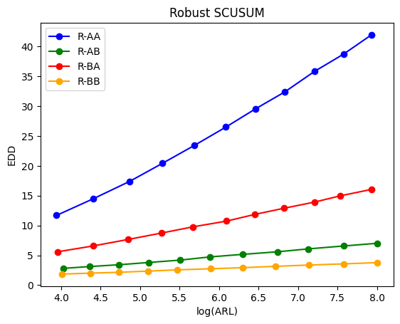
(a) Robust Tests

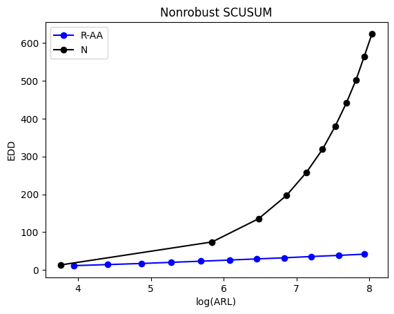
(b) Robust vs. Nonrobust

Figure 1: ARL vs EDD curves for the trials of Table II, averaged over 10,000 sample paths. (a) The RSCUSUM Algorithm (Algorithm 1) is simulated with various choices of $P_{\infty},P_{1}$; (b) The Nonrobust-SCUSUM algorithm (Algorithm 2) is simulated with $H_{\infty}=R_{\infty}^{B},H_{1}=R_{1}^{B}$ and is compared against a robust test from part (a).

Figure 1(a) demonstrates that the RSCUSUM Algorithm detects the change-point for many choices of $P_{\infty}\in\mathcal{G}_{\infty},P_{1}\in\mathcal{G}_{1}$. Consistent with Theorems VI.7 and VI.8, the EDD increases at most linearly with respect to a bound on log-ARL when ARL becomes arbitrarily large. The asymptotically linear relationship between ARL and EDD is consistent with that of the SCUSUM Algorithm when $P_{\infty},P_{1}$ are known precisely. Conversely, Figure 1(b) demonstrates that for a particular Nonrobust Algorithm applied to these uncertainty sets $\mathcal{G}_{\infty},\mathcal{G}_{1}$, the EDD increases exponentially with respect to a bound on log-ARL.

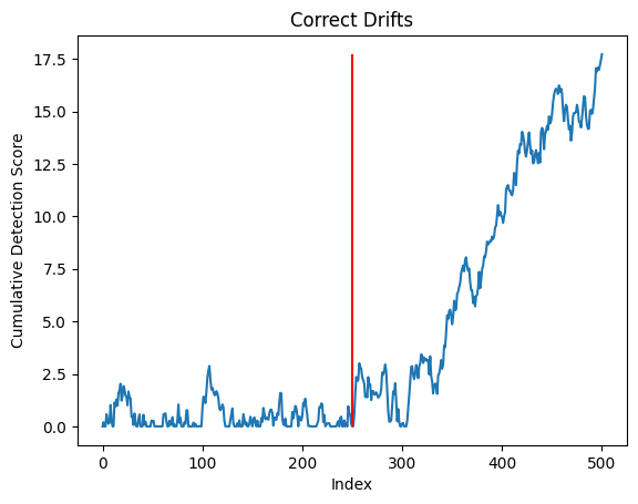
(a) Correct Drifts

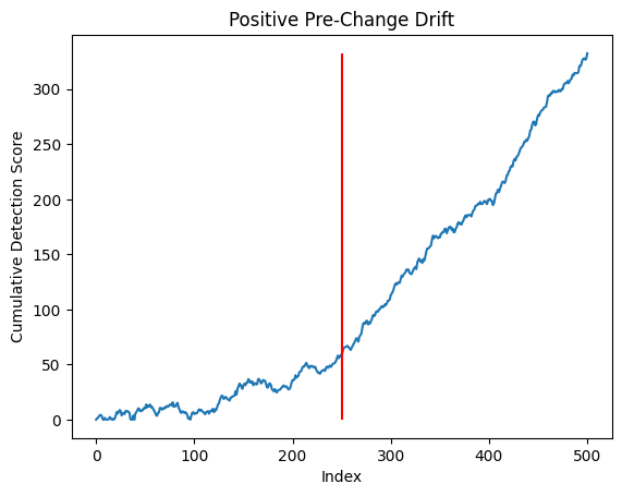
(b) Positive Pre-change Drift

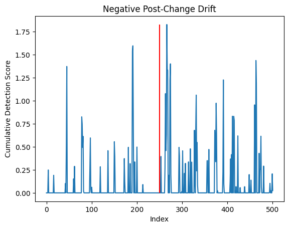
(c) Negative Post-change Drift

Figure 2: Select cumulative detection score paths. In each sample path, a change-point occurs at index 250, illustrated by a vertical red line. (a) A sample path from trial R-AA. (b) A sample path from trial N (Algorithm 2 with $H_{\infty}=R_{\infty}^{B},H_{1}=R_{1}^{B}$). (c) A sample path from a Nonrobust algorithm with $H_{\infty}=\mathcal{N}((-0.75,-0.75)^{T},V)$, $H_{1}=\mathcal{N}((1.5,1.5)^{T},V)$, $P_{\infty}=R_{\infty}^{A},P_{1}=R_{1}^{A}$. Note that this sample path is not from the experiment of Table II.

As shown in Lemma VI.5, the RSCUSUM Algorithm features negative pre-change drifts and positive post-change drifts. A sample path with these drifts is illustrated in Figure 2(a). The negative pre-change drift is essential to prevent false alarms; when the pre-change drift is positive (as is the case for the sample path in Figure 2(b) above), a very large detection threshold $\omega$ must be set in order to achieve a lengthy mean time to false alarm. Conversely, the positive post-change drifts reduce the detection delay; a negative post-change drift makes the detection delay very lengthy (as is the case for Figure 2(c)).

VIII-B Gauss-Bernoulli Restricted Boltzmann Machine

The Gauss-Bernoulli Restricted Boltzmann Machine (GBRBM) [19] is a model class that defines a probability density function over $\mathbb{R}^{v}$ and utilizes an $h$-dimensional latent vector. Parameterized by $W\in\mathbb{R}^{v\times h},b\in\mathbb{R}^{v}$, and $c\in\mathbb{R}^{h}$, the probability density function can be expressed as:

$$p(x)=\frac{1}{Z}\exp(-E(x))$$ (40)

where

$$E(x)=\frac{1}{2}\|x-b\|^{2}-\bigg{(}\text{Softplus}(W^{T}x+c)\bigg{)}\mathbf{1}_{h}.$$ (41)

Here, $\text{Softplus}(x)=\log(1+\exp(x))$ and $\mathbf{1}_{h}\in\mathbb{R}^{h}$ is a column vector of ones. Note that in this simulation, we assume the $\sigma$ parameter of [19] to be equal to one. Further:

$$Z=\int\exp(-E(x))dx.$$ (42)

Calculation of $Z$ is intractable for large $v,h$, so we instead leverage the unnormalized probability density function given by

$$\tilde{p}(x)=\exp(-E(x)).$$ (43)

The score function $\nabla_{x}\log p(x)$ can be expressed in closed-form in terms of $W,b,c$:

$$\nabla_{x}\log\tilde{p}(x)=b-x+W\text{Sigmoid}(W^{T}x+c)$$ (44)

where $\text{Sigmoid}(x)=\frac{1}{1+\exp(-x)}$.

We next demonstrate the robustness of RSCUSUM with Gauss-Bernoulli Restricted Boltzmann Machines (GBRBMs). For these GBRBMs, a single weight matrix $W^{*}\in\mathbb{R}^{10\times 8}$ and two bias vectors $v^{*}\in\mathbb{R}^{10},h^{*}\in\mathbb{R}^{8}$ are generated by setting their elements equal to draws from a scalar standard normal distribution. Several scalar adjustments are added to the weight matrix element-wise in order to construct several distinct GBRBMs.

Distribution	Weight Matrix	Visible Bias	Hidden Bias
$G_{\infty}^{0}$	$W^{*}-0.2$	$v^{*}$	$h^{*}$
$G_{\infty}^{1}$	$W^{*}-0.05$	$v^{*}$	$h^{*}$
$G_{1}^{0}$	$W^{*}$	$v^{*}$	$h^{*}$
$G_{1}^{1}$	$W^{*}+0.05$	$v^{*}$	$h^{*}$

TABLE III: Parameters of Distributions used in Numerical Simulations. Addition between matrices and scalars is element-wise.

These distinct GBRBMs define a finite basis for our two uncertainty classes. Specifically, we define $\mathcal{G}_{\infty}$ to be the convex hull of $\{G_{\infty}^{0},G_{\infty}^{1}\}$ and further define $\mathcal{G}_{1}$ to be the convex hull of $\{G_{1}^{0},G_{1}^{1}\}$:

$$\mathcal{G}_{\infty}=\bigg{\{}\sum_{i=1}^{m}\alpha_{i}G_{\infty}^{i}\,:\sum_{i=0}^{1}\alpha_{i}=1,\alpha_{i}\geq 0\bigg{\}},$$ (45)

$$\mathcal{G}_{1}=\bigg{\{}\sum_{i=1}^{m}\alpha_{i}G_{1}^{i}\,:\sum_{i=0}^{1}\alpha_{i}=1,\alpha_{i}\geq 0\bigg{\}}.$$ (46)

As each of the GBRBMs of Table III are linearly independent functions of $x$ when the weight matrices are distinct, the sets $\mathcal{G}_{\infty},\mathcal{G}_{1}$ are disjoint.

Here the pre-and post-change uncertainty classes $\mathcal{G}_{\infty},\mathcal{G}_{1}$ are constructed from finite bases (see Equation (27)). Using Theorem VII.1 and following the notation of Equation 28, we endeavor to learn the functions $\beta_{\infty}(x),\beta_{1}(x)$ that correspond to the least-favorable distributions among $\mathcal{G}_{\infty},\mathcal{G}_{1}$:

$$\nabla_{x}\log q_{\infty}(x)=\sum_{i=0}^{1}\beta_{\infty}^{i}(x)\nabla_{x}\log g_{\infty}^{i}(x):\sum_{i=1}^{m}\beta_{\infty}^{i}(x)=1,\;\beta_{\infty}^{i}(x)\geq 0,\;$$ (47)

$$\nabla_{x}\log q_{1}(x)=\sum_{i=0}^{1}\beta_{1}^{i}(x)\nabla_{x}\log g_{1}^{i}(x):\sum_{i=1}^{m}\beta_{1}^{i}(x)=1,\;\beta_{1}^{i}(x)\geq 0.\;$$ (48)

We use a neural network $\operatorname{Softmax}_{j}\circ f_{\infty}(x)$ to estimate $\beta_{\infty}^{j}(\cdot)$, specifically,

$$\beta_{\infty}^{j}(x)=\operatorname{Softmax}_{j}\circ f_{\infty}(x),$$

where $\operatorname{Softmax}_{j}$ denotes the $j$-th element of the Softmax function and where $f_{\infty}$ is given by a multi-layer perceptron (MLP) network. The architecture of this MLP is an input layer of dimension $v=10$, a single hidden layer of dimension $5$, and an output layer of dimension $2$. This MLP utilizes $\operatorname{ReLU}$ activation functions in hidden layers. The use of Softmax function ensures $\sum_{i=1}^{m}\beta_{\infty}^{i}(x)=1$ and $\beta_{\infty}^{i}(x)\geq 0$ for all $0\leq i\leq 1$. We further create a separate neural network $f_{1}(x)$ with the same architecture as that of $f_{\infty}$, also with $\operatorname{Softmax}$ at the output layer, to learn the functions $\beta_{1}^{i}$.

To learn the scores of $Q_{\infty},Q_{1}$, we train $f_{\infty}(\cdot),f_{1}(\cdot)$. During training, a set of $N=1,000$ particles $X_{1},...,X_{N}$ are initially sampled from an arbitrary distribution of the post-change set $\mathcal{G}_{1}$ using Gibbs sampling ([19]). The network is then trained to minimize the following loss function:

$$\frac{1}{N}\sum_{i=1}^{N}\bigg{\|}\sum_{j=0}^{1}\beta_{1}^{j}(X_{i})\nabla\log g_{1}^{j}(X_{i})-\sum_{k=0}^{1}\beta_{\infty}^{k}(X_{i})\nabla g_{\infty}^{k}(X_{i})\bigg{\|}_{2}^{2}.$$ (49)

After each epoch of training, the $N$ particles are repeatedly and iteratively updated via Langevin dynamics [19] (without Metropolis adjustment) $K$ times:

$$X_{i}\leftarrow X_{i}+\epsilon\sum_{j=0}^{1}\beta_{1}^{j}(X_{i})\nabla\log g_{1}^{j}(X_{i})+\sqrt{2\epsilon}t$$ (50)

where $t$ is a noise term sampled from $\mathcal{N}(0,I_{v})$ and where $\epsilon$ is a step size constant so that $X_{1},...,X_{N}$ remain samples of the distribution with score $\sum_{j=0}^{1}\beta_{1}^{j}(\cdot)\nabla\log g_{1}^{j}(\cdot)$ even as $\beta_{1}$ is updated. In this experiment, we let $K=1000,\epsilon=0.01$.

In Table IV, we report the average value $\frac{1}{N}\sum_{i=1}^{N}\beta_{\infty}^{j}(X_{i})$ and $\frac{1}{N}\sum_{i=1}^{N}\beta_{1}^{j}(X_{i})$ over the test samples $X_{1},\cdots X_{N}$ generated using the Langevin update step of Equation 50. In all cases the average value of $\beta_{\infty}^{j}(x),\beta_{1}^{j}(x)$ are very close to either $1$ or $0$. This gives strong evidence that the LFD is achieved by $Q_{\infty}=G_{\infty}^{1},Q_{1}=G_{1}^{0}$.

j	$0$	$1$
$\beta_{\infty}^{j}$	9.21e-5	9.99e-1
$\beta_{1}^{j}$	9.99e-1	6.22e-5

TABLE IV: Empirical average values of $\beta_{\infty}^{j}(X),\beta_{1}^{j}(X)$ over $N=1000$ test samples.

To proceed with Algorithm 1, we need a method of calculating the Hyvärinen scores $\mathcal{S}_{H}(\cdot,Q_{\infty}),\mathcal{S}_{H}(\cdot,Q_{1})$. These Hyvärinen scores are the sum of a gradient log-density, defined in Equations 47 and 48, along with a Laplacian term. To estimate the Laplacian term of a mixture of GBRBM distributions, we use Hutchinson’s Trick ([25, 22]):

$$\Delta_{x}\log q_{\infty}(x)=\mathbb{E}_{\epsilon\sim\mathcal{N}(0,I_{v})}[\epsilon^{T}\nabla_{x}f(x)\epsilon]=\mathbb{E}_{\epsilon\sim\mathcal{N}(0,I_{v})}[\epsilon^{T}\nabla_{x}(\epsilon^{T}f(x))]$$ (51)

with $f(x)=\sum_{i=1}^{m}\beta_{\infty}^{i}(x)\nabla_{x}\log g_{\infty}^{i}(x)$. In this simulation, we average over ten vectors $\epsilon$ sampled from $\mathcal{N}(0,I_{v})$ in order to estimate the expectation in Equation 51. We estimate $\Delta_{x}\log q_{1}(x)$ in a similar way.

Unlike the Gaussian Mixture Model case, there is not a convenient analytical method to verify that Assumption VI.1 holds. Thus, we verify it numerically: we sample $50,000$ samples from two choices of $P_{\infty}$ and estimate Fisher divergences:

$P_{\infty}$	$\mathbb{D}_{F}(P_{\infty}\|Q_{\infty})$	$\mathbb{D}_{F}(P_{\infty}\|Q_{1})$
$G_{\infty}^{0}$	2.91	3.69
$G_{\infty}^{1}$	1.10e-4	8.10e-1

TABLE V: Numerical estimation of the Fisher distances involved in Assumption VI.1. For each $P_{\infty}$ chosen, Assumption VI.1 holds. Fisher Divergences are estimated by averaging over 50,000 samples.

We can see that $\mathbb{D}_{F}(G_{\infty}^{1}\|Q_{\infty})$ is very close to zero, and this gives further evidence that the LFD $Q_{\infty}=G_{\infty}^{1}$. By Theorem VI.3, Assumption VI.1 holds for all $P_{\infty}\in\mathcal{G}_{\infty}$.

As with the Gaussian Mixture Model case, we first sample four different combinations of choices of $P_{\infty}\in\mathcal{G}_{\infty},P_{1}\in\mathcal{G}_{1}$ and show that the robust test consistently detects the change. Then, we compare the performance of the robust test to the performance of a nonrobust test.

Trial	$P_{\infty}$	$P_{1}$	Algorithm	Pre-Change Drift	Post-Change Drift
R-00	$G_{\infty}^{0}$	$G_{1}^{0}$	Algorithm 1	-2.58	0.341
R-01	$G_{\infty}^{0}$	$G_{1}^{1}$	Algorithm 1	-2.59	1.18
R-10	$G_{\infty}^{1}$	$G_{1}^{0}$	Algorithm 1	-0.339	0.342
R-11	$G_{\infty}^{1}$	$G_{1}^{1}$	Algorithm 1	-0.324	1.19
N	$G_{\infty}^{1}$	$G_{1}^{0}$	Algorithm 2	1.98	5.69

TABLE VI: The RSCUSUM Algorithm (Algorithm 1) is simulated for multiple choices of $P_{\infty},P_{1}$, and the Nonrobust-SCUSUM Algorithm (Algorithm 2) is simulated with $H_{\infty}=G_{\infty}^{0},H_{1}=G_{1}^{1}$. Drifts are averaged over 50,000 sample paths.

Trials R-00, R-01, R-10, and R-11 are robust and use the least-favorable distributions in the calculation of their instantaneous detection scores, while trial N is a nonrobust test and uses non-least-favorable distributions in the calculation of the instantaneous detection scores. As before, the robust drifts are negative before the change point and positive after the change point, but the nonrobust drifts are positive before the change point. Next, we vary the detection threshold $\omega$ and generate plots comparing mean time to false alarm with the expected detection delay:

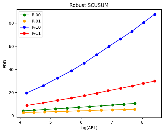
(a) Robust Tests

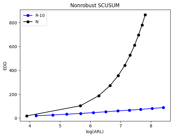
(b) Robust vs. Nonrobust

Figure 3: ARL vs EDD curves for the trials of Table VI, averaged over 10,000 sample paths. (a) The RSCUSUM Algorithm (Algorithm 1) is simulated with various choices of $P_{\infty},P_{1}$. (b) The Nonrobust-SCUSUM algorithm (Algorithm 2) is simulated with $H_{\infty}=G_{\infty}^{0},H_{1}=G_{1}^{1}$ and is compared against a robust test from part (a).

Figure 3(a) demonstrates that the RSCUSUM Algorithm detects the change-point for many choices of $P_{\infty}\in\mathcal{G}_{\infty},P_{1}\in\mathcal{G}_{1}$. Again, the log-ARL vs. EDD plot corroborates Theorems VI.7 and VI.8 as EDD increases at most linearly with log-ARL (as is the case for the SCUSUM Algorithm with precisely known $P_{\infty},P_{1}$). As before, a particular Nonrobust Algorithm applied to these uncertainty sets $\mathcal{G}_{\infty},\mathcal{G}_{1}$ produces an EDD that is exponential in log-ARL (Figure 3(b)).

IX Conclusion

In this work, we proposed the RSCUSUM algorithm. We defined the least favorable distributions in the sense of Fisher divergence. Using asymptotic analysis, we also analyzed the delay and false alarms of RSCUSUM in the sense of Lorden’s and Pollak’s metrics. We provided both theoretical and algorithmic methods for computing the least favorable distributions for unnormalized models. Numerical simulations were provided to demonstrate the performance of our robust algorithm.

Appendix A Selection of Appropriate Multiplier

The following proof and subsequent discussion use similar arguments as the proof of Lemma 2 of [15]. We note that the proofs are similar but not identical as the pre-change distribution $P_{\infty}$ may not be equal to the least favorable distribution $Q_{\infty}$.

Proof of Lemma VI.6.

Define the function $\rho:\mapsto h(\rho)$ given by

$$h(\rho)\overset{\Delta}{=}\mathbb{E}_{\infty}[\exp(z_{\rho}(X_{1}))]-1.$$

Observe that

$$h^{\prime}(\rho)\overset{\Delta}{=}\frac{dh}{d\rho}(\rho)=\mathbb{E}_{\infty}[(S_{\texttt{H}}(X_{1},Q_{\infty})-S_{\texttt{H}}(X_{1},Q_{1}))\exp(z_{\rho}(X_{1}))].$$

Note that $h(0)=0$, and $h^{\prime}(0)=\mathbb{D}_{F}(P_{\infty}\|Q_{\infty})-\mathbb{D}_{F}(P_{\infty}\|Q_{1})<0$ by Assumption VI.1. Next, we prove that either 1) there exists $\rho^{\star}\in(0,\infty)$ such that $h(\rho^{\star})=0$, or 2) for all $\rho>0$ we have $h(\rho)<0$.

Observe that

$$h^{\prime\prime}(\rho)\overset{\Delta}{=}\frac{d^{2}h}{d\rho}(\rho)=\mathbb{E}_{\infty}[(S_{\texttt{H}}(X_{1},Q_{\infty})-S_{\texttt{H}}(X_{1},Q_{1}))^{2}\exp(z_{\rho}(X_{1}))]\geq 0.$$

We claim that $h(\rho)$ is strictly convex, namely $h^{\prime\prime}(\rho)>0$ for all $\rho\in[0,\infty)$. Suppose $h^{\prime\prime}(\rho)=0$ for some $\rho\geq 0$, we must have $S_{\texttt{H}}(X_{1},Q_{\infty})-S_{\texttt{H}}(X_{1},Q_{1})=0$ almost surely. This implies that $\mathbb{E}_{\infty}[(S_{\texttt{H}}(X_{1},Q_{\infty})-S_{\texttt{H}}(X_{1},Q_{1}))]=0$ which in turn gives $\mathbb{D}_{F}(P_{\infty}\|Q_{\infty})-\mathbb{D}_{F}(P_{\infty}\|Q_{1})=0$, violating Assumption VI.1. Thus, $h(\rho)$ is strictly convex and $h^{\prime}(\rho)$ is strictly increasing.

Here, we recognize two cases: either 1) $h(\rho)$ have at most one global minimum in $(0,\infty)$, or 2) it is strictly decreasing in $[0,\infty)$. We will show that the second case is degenerate that is of no practical interest.

• Case 1: If the global minimum of $h(\rho)$ is attained at $a\in(0,\infty)$, then $h^{\prime}(a)=0$. Since $h^{\prime}(0)<0$ and $h(0)=0$, the global minimum $h(a)<0$. Since $h^{\prime}(\rho)$ is strictly increasing, we can choose $b>a$ and conclude that $h^{\prime}(\rho)>h^{\prime}(b)>h^{\prime}(a)=0$ for all $\rho>b$. It follows that $\lim_{\rho\rightarrow\infty}h(\rho)=+\infty$. Combining this with the continuity of $h(\rho)$, we conclude that $h(\rho^{*})=0$ for some $\rho^{*}\in(0,\infty)$ and any value of $\rho\in(0,\rho^{*}]$ satisfies Inequality (10).

  Note that in this case, we must have $P_{\infty}\left(S_{\texttt{H}}(X_{1},Q_{\infty})-S_{\texttt{H}}(X_{1},Q_{1})\geq c\right)>0$, for some $c>0$. Otherwise, we have $P_{\infty}\left(S_{\texttt{H}}(X_{1},Q_{\infty})-S_{\texttt{H}}(X_{1},Q_{1})\leq 0\right)=1$. This implies that $P_{\infty}(z_{\rho}(X_{1})\leq 0)=1$, or equivalently $\mathbb{E}_{\infty}[\exp(z_{\rho}(X_{1}))]<1$ for all $\rho>0$, and therefore leads to Case 2: $h(\rho)<0$ for all $\rho>0$. Here, $\mathbb{E}_{\infty}[\exp(z_{\rho}(X_{1}))]\neq 1$ since $P_{\infty}(S_{\texttt{H}}(X_{1},Q_{\infty})-S_{\texttt{H}}(X_{1},Q_{1})=0)<1$; otherwise $P_{\infty}(S_{\texttt{H}}(X_{1},Q_{\infty})-S_{\texttt{H}}(X_{1},Q_{1})=0)=1$, and then $\mathbb{E}_{\infty}[S_{\texttt{H}}(X_{1},Q_{\infty})-S_{\texttt{H}}(X_{1},Q_{1})]=\mathbb{D}_{F}(P_{\infty}\|Q_{\infty})-\mathbb{D}_{F}(P_{\infty}\|Q_{1})=0$, causing the same contradiction to Assumption VI.1.

• Case 2: If $h(\rho)$ is strictly decreasing in $(0,\infty)$, then any $\rho\in(0,\infty)$ satisfies Inequality (10). As discussed before, in this case, we must have $P_{\infty}\left(S_{\texttt{H}}(X_{1},Q_{\infty})-S_{\texttt{H}}(X_{1},Q_{1})\leq 0\right)=1$. Equivalently, all the increments of the RSCUSUM detection score are non-positive under the pre-change distribution, and $P_{\infty}(Z(n)=0)=1$ for all $n$. Accordingly, $\mathbb{E}_{\infty}[T_{\textit{RSCUSUM}}]=+\infty$. When there occurs change (under measure $Q_{1}$), we also observe that RSCUSUM can get close to detecting the change-point instantaneously as $\rho$ is chosen arbitrarily large. Obviously, this case is of no practical interest.

∎

In practice, it is possible to use $m$ past samples $\mathbf{X}_{[-m+1,0]}$ to estimate the value of $\rho$. In particular, $\rho$ can be chosen as the positive root of the function $\rho\to\tilde{h}(\rho)$ given by

$$\tilde{h}(\rho)\overset{\Delta}{=}\frac{1}{m}\sum_{i=1}^{m}[\exp(z_{\rho}(X_{i-m}))]-1.$$

By Lemma VI.6 and its related technical discussions, the above equation has a root greater than zero with a high probability if $m$ is sufficiently large. In the case that $\rho$ is not chosen properly, the algorithm remains implementable but optimal performance of detection delay is not guaranteed.

It is worth noting that although our core results hold for a pre-selected $\rho$ that satisfied the condition discussed in Lemma VI.6, the effect of choosing any other $\rho^{\prime}$ amounts to the scaling of all the increments of RSCUSUM by a constant factor of $\rho^{\prime}/\rho$. This means that all of these results still hold adjusted for this scale factor. The result of Theorem VI.7 can be modified to be written as

$$\mathbb{E}_{\infty}[T_{\texttt{RSCUSUM}}]\geq\exp\left\{\frac{\rho\omega}{\max(\rho,\rho^{\prime})}\right\},$$

for any $\rho^{\prime}>0$.

It is easy to see that this scaling will change the statement of Theorem VI.8 accordingly to

$$\mathbb{E}_{1}[T_{\texttt{RSCUSUM}}]\sim\frac{\max(\rho,\rho^{\prime})}{\rho}\frac{\log\gamma}{\rho^{\prime}(\mathbb{D}_{\texttt{F}}(P_{1}\|Q_{\infty})-\mathbb{D}_{\texttt{F}}(P_{1}\|Q_{1}))},$$

as $\gamma\to\infty$.

In order to have the strongest results, we must choose $\rho$ as close to $\rho^{*}$ as possible.

Appendix B Proofs of Delay and False Alarm Theorems

The theoretical analysis for delay and false alarms is analogous to the analysis from [15]. We again note that the proofs are similar but not identical as the pre-change distribution $P_{\infty}$ may not be equal to the least favorable distribution $Q_{\infty}$.

B-A Proof of Theorem VI.7

Proof.

We prove the result in multiple steps and follow the proof technique of [15], which in turn uses the proof technique given in [9].

1. Define

   $$Z_{\rho}(0)=0,$$

   $$Z_{\rho}(n)\overset{\Delta}{=}(Z_{\rho}(n-1)+z_{\rho}(X_{1}))^{+},\;\forall n\geq 1,$$

   where

   $$z_{\rho}(x)=\rho\left(\mathcal{S}_{\texttt{H}}(x,Q_{\infty})-\mathcal{S}_{\texttt{H}}(x,Q_{1})\right),$$ (52)

   where $\mathcal{S}_{\texttt{H}}(x,Q_{\infty})$ and $\mathcal{S}_{\texttt{H}}(x,Q_{1})$ are respectively the Hyvärinen score functions of $Q_{\infty}$ and $Q_{1}$, the LFD pair. Also, note that $\rho$ satisfies

   $$\mathbb{E}_{\infty}[\exp(z_{\rho}(X_{1}))]\leq 1,$$ (53)

   Note that

   $$T_{\texttt{RSCUSUM}}=\inf\{n\geq 1:Z_{\rho}(n)\geq\omega\rho\}.$$ (54)

   For convenience, define $\omega^{\prime}\overset{\Delta}{=}\omega\rho$.

2. We next construct a non-negative martingale with mean $1$ under the measure $P_{\infty}$. Define a new instantaneous score function $x\mapsto\tilde{z}_{\rho}(x)$ given by

   $$\tilde{z}_{\rho}(x)\overset{\Delta}{=}z_{\rho}(x)+\delta,$$

   where

   $$\delta\overset{\Delta}{=}-\log\biggr{(}\mathbb{E}_{\infty}\left[\exp(z_{\rho}(X_{1}))\right]\biggr{)}.$$

   Further define the sequence

   $$\tilde{G}_{n}\overset{\Delta}{=}\exp\biggr{(}\sum_{k=1}^{n}\tilde{z}_{\rho}(X_{k})\biggr{)},\;\forall n\geq 1.$$

   Since $\mathbb{E}_{\infty}\left[\exp(z_{\rho}(X_{1}))\right]\leq 1$, $\delta\geq 0$.

   Suppose $X_{1},X_{2},\ldots$ are i.i.d according to $P_{\infty}$ (no change occurs). Then,

   $$\mathbb{E}_{\infty}\left[\tilde{G}_{n+1}\mid\mathcal{F}_{n}\right]=\tilde{G}_{n}\mathbb{E}_{\infty}[\exp(\tilde{z}_{\rho}(X_{n+1}))]=\tilde{G}_{n}e^{\delta}\mathbb{E}_{\infty}[\exp(z_{\rho}(X_{n+1}))]=\tilde{G}_{n},$$

   and

   $$\mathbb{E}_{\infty}[\tilde{G}_{n}] =\mathbb{E}_{\infty}\left[\exp\left(\sum_{i=1}^{n}(z_{\rho}(X_{i})+\delta)\right)\right]=e^{n\delta}\prod_{i=1}^{n}\mathbb{E}_{\infty}[\exp(z_{\rho}(X_{i}))]=1.$$ (55)

   Thus, under the measure $P_{\infty}$, $\{\tilde{G}_{n}\}_{n\geq 1}$ is a non-negative martingale with the mean $\mathbb{E}_{\infty}[\tilde{G}_{1}]=1$.

3. We next examine the new stopping rule

   $$\tilde{T}_{\texttt{RSCUSUM}}=\inf\left\{n\geq 1:\max_{1\leq k\leq n}\sum_{i=k}^{n}\tilde{z}_{\rho}(X_{i})\geq\omega^{\prime}\right\},$$

   where $\tilde{z}_{\rho}(X_{i})=z_{\rho}(X_{i})+\delta$. Since $\delta\geq 0$, we have

   $$T_{\texttt{RSCUSUM}}\geq\tilde{T}_{\texttt{RSCUSUM}},$$

   and $\mathbb{E}_{\infty}[T_{\texttt{RSCUSUM}}]\geq\mathbb{E}_{\infty}[\tilde{T}_{\texttt{RSCUSUM}}]$. Thus, it is sufficient to lower bound the modified stopping time $\tilde{T}_{\texttt{RSCUSUM}}$.

4. By Jensen’s inequality,

   $$\mathbb{E}_{\infty}[\exp(z_{\rho}(X_{1}))]\geq\exp\left(\mathbb{E}_{\infty}[z_{\rho}(X_{1})]\right),$$ (56)

   with equality holds if and only if $z_{\rho}(X_{1})=c$ almost surely, where $c$ is some constant. Suppose the equality of Equation (56) holds, then

   $$\rho(\mathbb{D}_{F}(P_{\infty}\|Q_{\infty})-\mathbb{D}_{F}(P_{\infty}\|Q_{1})) =\mathbb{E}_{\infty}[z_{\rho}(X_{1})]=c=\mathbb{E}_{1}[z_{\rho}(X_{1})]\geq\rho\mathbb{D}_{F}(Q_{1}\|Q_{\infty})$$

   Recalling Assumption VI.1 and dividing through by $\rho>0$, we know that $0>\mathbb{D}_{F}(P_{\infty}\|Q_{\infty})-\mathbb{D}_{F}(P_{\infty}\|Q_{1})\geq\mathbb{D}_{F}(Q_{1}\|Q_{\infty})\geq 0$, the last inequality a result of the fact that the Fisher distance is nonnegative. Thus, the inequality of Equation (56) is strict. Continuing from Equation 55:

   $$1= e^{n\delta}\prod_{i=1}^{n}\mathbb{E}_{\infty}[\exp(z_{\rho}(X_{i}))]$$

   $$e^{-n\delta}= \bigg{(}\mathbb{E}_{\infty}[\exp(z_{\rho}(X_{1}))]\bigg{)}^{n}$$

   $$e^{-\delta}= \mathbb{E}_{\infty}[\exp(z_{\rho}(X_{1}))]>\exp(\mathbb{E}_{\infty}(z_{\rho}(X_{1}))),$$

   where the strictness of the final inequality follows from the strictness of the inequality in Equation (56). Taking the log, we have that $\delta<-\rho(\mathbb{D}_{F}(P_{\infty}\|Q_{\infty})-\mathbb{D}_{F}(P_{\infty}\|Q_{1}))$, so

   $$\mathbb{E}_{\infty}[\tilde{z}_{\rho}(X_{i})]=\mathbb{E}_{\infty}[z_{\rho}(X_{i})]+\delta<\rho(\mathbb{D}_{F}(P_{\infty}\|Q_{\infty})-\mathbb{D}_{F}(P_{\infty}\|Q_{1}))-\rho(\mathbb{D}_{F}(P_{\infty}\|Q_{\infty})-\mathbb{D}_{F}(P_{\infty}\|Q_{1}))=0$$

   so we know that $\tilde{z}_{\rho}(X_{i})$ has a negative drift under the $P_{\infty}$ law. Thus, $\tilde{T}_{\texttt{RSCUSUM}}$ is not trivial.

5. Define a sequence of stopping times:

   $$\eta_{0} =0,$$

   $$\eta_{1} =\inf\left\{t:\sum_{i=1}^{t}\tilde{z}_{\rho}(X_{i})<0\right\},$$

   $$\eta_{k+1} =\inf\left\{t>\eta_{k}:\sum_{i=\eta_{k}+1}^{t}\tilde{z}_{\rho}(X_{i})<0\right\},\;\text{for}\;k\geq 1.$$

   Furthermore, let

   $$M\overset{\Delta}{=}\inf\biggl{\{}k\geq 0:\eta_{k}<\infty\;\text{and}\;\sum_{i=\eta_{k}+1}^{n}\tilde{z}_{\rho}(X_{i})\geq\omega^{\prime}\;\text{for some}\;n>\eta_{k}\biggr{\}}.$$ (57)

   Then, it follows from the definitions that

   $$\tilde{T}_{\texttt{RSCUSUM}}\geq M.$$

   Hence, it is enough to lower bound $\mathbb{E}_{\infty}[M]$. To this end, we obtain a lower bound on the probability $P_{\infty}(M>k)$ and then utilize the identity $\mathbb{E}_{\infty}[M]=\sum_{k=0}^{\infty}P_{\infty}(M>k)$.

6. For the probability $P_{\infty}(M>k)$, note that since the event $\{M<k\}$ is $\mathcal{F}_{\eta_{k}}-$measurable,

   $$\begin{split}P_{\infty}(M>k)&=\mathbb{E}_{\infty}[\mathbb{I}_{\{M>k\}}]=\mathbb{E}_{\infty}[\mathbb{I}_{\{M>k\}}\mathbb{I}_{\{M\geq k\}}]=\mathbb{E}_{\infty}\left[\mathbb{E}_{\infty}[\mathbb{I}_{\{M>k\}}\mathbb{I}_{\{M\geq k\}}|\mathcal{F}_{\eta_{k}}]\right]\\ &=\mathbb{E}_{\infty}[P_{\infty}(M\geq k+1\mid\mathcal{F}_{\eta_{k}})\mathbb{I}_{\{M\geq k\}}].\end{split}$$ (58)

   Next, we bound the probability $P_{\infty}(M\geq k+1\mid\mathcal{F}_{\eta_{k}})$. For this, note that

   $$P_{\infty}(M\geq k+1\mid\mathcal{F}_{\eta_{k}})=1-P_{\infty}\left(\sum_{i=\eta_{k}+1}^{n}\tilde{z}_{\rho}(X_{i})\geq\omega^{\prime}\;\text{for some}\;n>\eta_{k}\mid\mathcal{F}_{\eta_{k}}\right).$$ (59)

   Now, note that due to the independence of the observations,

   $$P_{\infty}\left(\sum_{i=\eta_{k}+1}^{n}\tilde{z}_{\rho}(X_{i})\geq\omega^{\prime}\;\text{for some}\;n>\eta_{k}\mid\mathcal{F}_{\eta_{k}}\right)=P_{\infty}\left(\sum_{i=1}^{n}\tilde{z}_{\rho}(X_{i})\geq\omega^{\prime}\;\text{for some}\;n\right).$$

   Next, for the right-hand side of the above equation, we have

   $$\begin{split}P_{\infty}\left(\sum_{i=1}^{n}\tilde{z}_{\rho}(X_{i})\geq\omega^{\prime}\;\text{for some}\;n\right)&=\lim_{m\rightarrow\infty}P_{\infty}\left(\max_{n:n\leq m}\sum_{i=1}^{n}\tilde{z}_{\rho}(X_{i})>\omega^{\prime}\right)\\ &=\lim_{m\rightarrow\infty}P_{\infty}\left(\max_{n:n\leq m}\exp\left(\sum_{i=1}^{n}\tilde{z}_{\rho}(X_{i})\right)>e^{\omega^{\prime}}\right)\\ &=\lim_{m\rightarrow\infty}P_{\infty}\left(\max_{n:n\leq m}\tilde{G}_{n}>e^{\omega^{\prime}}\right).\end{split}$$

   Since $\{\tilde{G}_{n}\}_{n\geq 1}$ is a nonnegative martingale under $P_{\infty}$ with mean 1, by Doob’s submartingale inequality [26], we have:

   $$P_{\infty}\left(\max_{n:n\leq m}\tilde{G}_{n}>e^{\omega^{\prime}}\right)\leq\frac{\mathbb{E}[\tilde{G}_{m}]}{e^{\omega^{\prime}}}=e^{-\omega^{\prime}}$$ (60)

   Thus,

   $$\begin{split}P_{\infty}(M\geq k+1\mid\mathcal{F}_{\eta_{k}})&=1-P_{\infty}\left(\sum_{i=\eta_{k}+1}^{n}\tilde{z}_{\rho}(X_{i})\geq\omega^{\prime}\;\text{for some}\;n>\eta_{k}\mid\mathcal{F}_{\eta_{k}}\right)\\ &=1-P_{\infty}\left(\sum_{i=1}^{n}\tilde{z}_{\rho}(X_{i})\geq\omega^{\prime}\;\text{for some}\;n\right)\\ &=1-\lim_{m\rightarrow\infty}P_{\infty}\left(\max_{n:n\leq m}\tilde{G}_{n}>e^{\omega^{\prime}}\right)\geq 1-e^{\omega^{\prime}}.\end{split}$$ (61)

7. Finally, from (58), we have

   $$\begin{split}P_{\infty}(M>k)&=\mathbb{E}_{\infty}[P_{\infty}(M\geq k+1\mid\mathcal{F}_{\eta_{k}})\mathbb{I}_{\{M\geq k\}}]\\ &\geq(1-e^{\omega^{\prime}})P_{\infty}(M>k-1)\\ &\geq(1-e^{\omega^{\prime}})^{2}P_{\infty}(M>k-2)\\ &\geq\dots\geq(1-e^{\omega^{\prime}})^{k}\end{split}$$ (62)

   Using (62), we arrive at a geometric series:

   $$\mathbb{E}_{\infty}[M]=\sum_{k=0}^{\infty}P_{\infty}(M>k)\geq\sum_{k=0}^{\infty}(1-e^{-\omega^{\prime}})^{k}=e^{\omega^{\prime}}.$$

   Thus, we conclude that

   $$\mathbb{E}_{\infty}[T_{\texttt{RSCUSUM}}]\geq\mathbb{E}_{\infty}[\tilde{T}_{\texttt{RSCUSUM}}]\geq\mathbb{E}_{\infty}[M]\geq e^{\omega^{\prime}}=e^{\rho\omega}.$$

∎

B-B Proof of Theorem VI.8

The following proof uses similar arguments to the proof of Theorem 4 of [15]. We first introduce a technical definition in order to apply Corollary 2.2 of [18] to the proof of Theorem VI.8.

Definition B.1.

A distribution $P$ on the Borel sets of $(-\infty,\infty)$ is said to be arithmetic if and only if it concentrates on a set of points of the form $\pm nd$, where $d>0$ and $n=1,2,\ldots$.

Remark B.2.

Any probability measure that is absolutely continuous with respect to the Lebesgue measure is non-arithmetic.

Proof.

Consider the random walk that is defined by

$$Z^{\prime}(n)=\sum_{i=1}^{n}z(X_{i}),\;\text{for}\;n\geq 1.$$

We examine another stopping time that is given by

$$T_{\texttt{RSCUSUM}}^{\prime}\overset{\Delta}{=}\inf\{n\geq 1:Z^{\prime}(n)\geq\omega\}.$$

Next, for any $\omega$, define $R_{\omega}$ on $\{T_{\texttt{RSCUSUM}}^{\prime}<\infty\}$ by

$$R_{\omega}\overset{\Delta}{=}Z^{\prime}(T_{\texttt{RSCUSUM}}^{\prime})-\omega.$$

$R_{\omega}$ is the excess of the random walk over a stopping threshold $\omega$ at the stopping time $T_{\texttt{RSCUSUM}}^{\prime}$. Suppose the change-point $\nu=1$, then $X_{1},X_{2},\ldots,$ are i.i.d. following the distribution $Q_{1}$. Let $\mu$ and $\sigma^{2}$ respectively denote the mean $\mathbb{E}_{1}[z(X_{1})]$ and the variance $\text{Var}_{1}[z(X_{1})]$. Note that

$$\mu=\mathbb{E}_{1}[z(X_{1})]=\mathbb{D}_{\texttt{F}}(P_{1}\|Q_{\infty})-\mathbb{D}_{\texttt{F}}(P_{1}\|Q_{1})>0,$$

and

$$\sigma^{2}=\text{Var}_{1}[z(X_{1})]=\mathbb{E}_{1}[z(X_{1})^{2}]-\left(\mathbb{D}_{\texttt{F}}(P_{1}\|Q_{\infty})-\mathbb{D}_{\texttt{F}}(P_{1}\|Q_{1})\right)^{2}.$$

Under the mild regularity conditions given by [16], which we assume in Assumption V.3:

$$\mathbb{E}_{1}[\mathcal{S}_{\texttt{H}}(X_{1},Q_{\infty})^{2}]<\infty,\;\text{and}$$

$$\mathbb{E}_{1}[\mathcal{S}_{\texttt{H}}(X_{1},Q_{1})^{2}]<\infty.$$

Therefore, by [27] Theorem 1,

$$\sup_{\omega\geq 0}\mathbb{E}_{1}[R_{\omega}]\leq\frac{\mathbb{E}_{1}[(z(X_{1})^{+})^{2}]}{\mathbb{E}_{1}[z(X_{1})]}\leq\frac{\mathbb{E}_{1}[(z(X_{1}))^{2}]}{\mathbb{E}_{1}[z(X_{1})]}=\frac{\mu^{2}+\sigma^{2}}{\mu},$$

where $z(X)^{+}=\max(z(X),0)$. Additionally, $Q_{1}$ must be non-arithmetic in order to have Hyvärinen scores well-defined. Hence, by [18] Corollary 2.2.,

$$\mathbb{E}_{1}[T^{\prime}_{\texttt{RSCUSUM}}]=\frac{\omega}{\mu}+\frac{\mathbb{E}_{1}[{R_{\omega}}]}{\mu}\leq\frac{\omega}{\mu}+\frac{\mu^{2}+\sigma^{2}}{\mu^{2}},\;\forall\omega\geq 0.$$

Observe that for any $n$, $Z^{\prime}(n)\leq Z(n)$, and therefore $T_{\texttt{RSCUSUM}}\leq T_{\texttt{RSCUSUM}}^{\prime}$. Thus,

$$\mathbb{E}_{1}[T_{\texttt{RSCUSUM}}]\leq\mathbb{E}_{1}[T_{\texttt{RSCUSUM}}^{\prime}]\leq\frac{\omega}{\mu}+\frac{\mu^{2}+\sigma^{2}}{\mu^{2}},\;\forall\omega\geq 0.$$ (63)

The contribution of the term $\frac{\mu^{2}+\sigma^{2}}{\mu^{2}}$ becomes negligible as $\omega\rightarrow\infty$. In addition, we have

$$\mathcal{L}_{\texttt{CADD}}(T_{\texttt{RSCUSUM}})=\mathbb{E}_{1}[T_{\texttt{RSCUSUM}}]-1.$$

Thus, we conclude that

$$\mathcal{L}_{\texttt{CADD}}(T_{\texttt{RSCUSUM}})\sim\frac{\omega}{\mathbb{D}_{\texttt{F}}(P_{1}\|Q_{\infty})-\mathbb{D}_{\texttt{F}}(P_{1}\|Q_{1})}.$$

Similar arguments applies for $\mathcal{L}_{\texttt{WADD}}(T_{\texttt{RSCUSUM}})$. ∎

References

• [1] V. V. Veeravalli and T. Banerjee, “Quickest change detection,” in Academic press library in signal processing.   Elsevier, 2014, vol. 3, pp. 209–255.
• [2] M. Basseville, I. V. Nikiforov et al., Detection of abrupt changes: theory and application.   prentice Hall Englewood Cliffs, 1993, vol. 104.
• [3] H. V. Poor and O. Hadjiliadis, Quickest detection.   Cambridge University Press, 2008.
• [4] A. Tartakovsky, I. Nikiforov, and M. Basseville, Sequential analysis: Hypothesis testing and changepoint detection.   CRC Press, 2014.
• [5] A. N. Shiryaev, “On optimum methods in quickest detection problems,” Theory Probab. Appl., vol. 8, no. 1, pp. 22–46, 1963.
• [6] A. G. Tartakovsky and V. V. Veeravalli, “General asymptotic bayesian theory of quickest change detection,” Theory of Probability & Its Applications, vol. 49, no. 3, pp. 458–497, 2005.
• [7] G. Lorden, “Procedures for reacting to a change in distribution,” Ann. Math. Stat., pp. 1897–1908, 1971.
• [8] G. V. Moustakides, “Optimal stopping times for detecting changes in distributions,” Ann. Stat., vol. 14, no. 4, pp. 1379–1387, 1986.
• [9] T. L. Lai, “Information bounds and quick detection of parameter changes in stochastic systems,” IEEE Trans. Inf. Theory, vol. 44, no. 7, pp. 2917–2929, 1998.
• [10] E. Page, “A test for a change in a parameter occurring at an unknown point,” Biometrika, vol. 42, no. 3/4, pp. 523–527, 1955.
• [11] M. Pollak, “Optimal detection of a change in distribution,” Ann. Stat., pp. 206–227, 1985.
• [12] S. Roberts, “A comparison of some control chart procedures,” Technometrics, vol. 8, no. 3, pp. 411–430, 1966.
• [13] Y. LeCun, S. Chopra, R. Hadsell, M. Ranzato, and F. Huang, “A tutorial on energy-based learning,” in Predicting structured data.   The MIT Press, 2006, vol. 1.
• [14] Y. Song, J. Sohl-Dickstein, D. P. Kingma, A. Kumar, S. Ermon, and B. Poole, “Score-based generative modeling through stochastic differential equations,” arXiv preprint arXiv:2011.13456, 2020.
• [15] S. Wu, E. Diao, T. Banerjee, J. Ding, and V. Tarokh, “Quickest change detection for unnormalized statistical models,” IEEE Transactions on Information Theory, 2023.
• [16] A. Hyvärinen, “Estimation of non-normalized statistical models by score matching.” J. Mach. Learn. Res., vol. 6, no. 4, 2005.
• [17] J. Unnikrishnan, V. V. Veeravalli, and S. P. Meyn, “Minimax robust quickest change detection,” IEEE Transactions on Information Theory, vol. 57, no. 3, pp. 1604–1614, 2011.
• [18] M. Woodroofe, Nonlinear renewal theory in sequential analysis.   SIAM, 1982.
• [19] R. Liao, S. Kornblith, M. Ren, D. J. Fleet, and G. Hinton, “Gaussian-bernoulli rbms without tears,” 2022.
• [20] Y. Song and S. Ermon, “Generative modeling by estimating gradients of the data distribution,” Advances in Neural Information Processing Systems (NeurIPS), 2019.
• [21] P. Vincent, “A connection between score matching and denoising autoencoders,” Neural computation, vol. 23, no. 7, pp. 1661–1674, 2011.
• [22] S. Wu, E. Diao, K. Elkhalil, J. Ding, and V. Tarokh, “Score-based hypothesis testing for unnormalized models,” IEEE Access, vol. 10, pp. 71 936–71 950, 2022.
• [23] S. Shao, P. E. Jacob, J. Ding, and V. Tarokh, “Bayesian model comparison with the hyvärinen score: Computation and consistency,” Journal of the American Statistical Association, vol. 114, no. 528, pp. 1826–1837, 2019.
• [24] J. Ding, R. Calderbank, and V. Tarokh, “Gradient information for representation and modeling,” Advances in Neural Information Processing Systems, vol. 32, 2019.
• [25] M. Hutchinson, “A stochastic estimator of the trace of the influence matrix for laplacian smoothing splines,” Communication in Statistics- Simulation and Computation, vol. 18, pp. 1059–1076, 01 1989.
• [26] J. L. Doob, Stochastic processes.   Wiley New York, 1953, vol. 7.
• [27] G. Lorden, “On excess over the boundary,” Ann. Math. Stat., vol. 41, no. 2, pp. 520–527, 1970.