Deep Reinforcement Learning with Symmetric Data Augmentation Applied for Aircraft Lateral Attitude Tracking Control
Abstract
Symmetry is an essential property in some dynamical systems that can be exploited for state transition prediction and control policy optimization. This paper develops two symmetry-integrated Reinforcement Learning (RL) algorithms based on standard Deep Deterministic Policy Gradient (DDPG), which leverage environment symmetry to augment explored transition samples of a Markov Decision Process(MDP). The firstly developed algorithm is named as Deep Deterministic Policy Gradient with Symmetric Data Augmentation (DDPG-SDA), which enriches dataset of standard DDPG algorithm by symmetric data augmentation method under symmetry assumption of a dynamical system. To further improve sample utilization efficiency, the second developed RL algorithm incorporates one extra critic network, which is independently trained with augmented dataset. A two-step approximate policy iteration method is proposed to integrate training for two critic networks and one actor network. The resulting RL algorithm is named as Deep Deterministic Policy Gradient with Symmetric Critic Augmentation (DDPG-SCA). Simulation results demonstrate enhanced sample efficiency and tracking performance of developed two RL algorithms in aircraft lateral tracking control task.
Index Terms-reinforcement learning, symmetry, data augmentation, approximate policy iteration, flight control.
I INTRODUCTION
Symmetry property commonly exists in the motions of various mechanical systems, such as aircrafts[1], cars[2] and robotic arms[3]. The common cognition for symmetry property is that the trajectories are symmetric with respect to a reference plane. To be more specific, the knowledge of the trajectory in one symmetric side is predicable according to the knowledge of the trajectory in the other side. A simple case of cart-pole motion with symmetry is seen in Ref [4].
Mathematical models for a dynamical system are mainly categorized as Ordinary Differential Equation(ODE) and Markov Decision Process(MDP). ODE describes state transition by first-derivative equations of state variables, while MDP describes state transition by multi-step transitional state samples. Furthermore, MDP evaluates the state transition samples with a reward function, and state trajectories with a state/state-action value function. Symmetry in ODE-based dynamical system is studies in various methods. Ref[5] uses Lie group operator to calculate the transformation function, which assists to find the symmetric solutions of original equations. Ref[6] uses Koopman theory to derive symmetry maps of a nonlinear dynamical system. In Ref[7], theoretical analysis is provided on the interplay of symmetries and stability in nonlinear dynamical systems. To consider symmetry in MDP model, Ref[8] derives symmetry from equivalence relation between states. Ref[4] derives symmetry from homomorphism, which is a more rigorously defined property of a MDP. In Ref[9, 10], group symmetry property is used to construct equivariant layers in network structure.
The state-of-the-art works on integrating model symmetry into Reinforcement Learning(RL) algorithms use three main approaches:(1) sample augmentation with symmetry[16, 17, 18, 19, 20, 21, 22, 23, 24] (2) loss function extension with symmetry[6, 11, 12, 13, 14, 15] and (3) network architecture modification with symmetry[12, 20, 25, 26]. Sample augmentation with symmetry is based on the assumption that symmetry holds in the whole environment to be explored by a RL agent. For a dynamical system, the state trajectory executed by an exploration policy always has a symmetric counterpart. Therefore, samples collected from explored trajectory can be used to calculate samples from symmetric trajectory without actually executing the exploration policy. For a RL agent, the number of state transition samples is doubled in this way so that sample efficiency is improved. Especially when the exploration is costly for some online-operated mechanical systems, such as aircraft. In [16], the explored state-action pairs are mirrored in Maximum aposteriori Policy Optimization(MPO) algorithm for the agent to learn faster. In [17, 18], the expert-guided detection method is used to verify symmetries by assuming the system dynamics is invariant. The detected symmetries are then used to augment explored dataset in simple experiments(Grid, Cart-pole, Acrobot), verifying a data-efficient learning of the environment transition functions. In [19], the Lie point symmetry group is used to augment samples in neural Partial Differential Equation (PDE) solver. In [20, 21], the generalization bounds for data augmentation and equivariant networks using symmetry are derived, which describes their effects on learning in a theoretical framework. In [22, 23], symmetry is combined with experience replay technique for data augmentation. In [24], the equivariance set of a MDP model is learned by using an equivariance loss in dynamical model training. The equivariance set is then used for data augmentation in offline RL. In [6], a pre-trained forward model is used for Koopman latent representation of equivariant dynamical systems, leading to a symmetry transformation for data augmentation in offline Q-learning.
Loss extension with symmetry method considers a symmetry loss term in loss function of critic network or actor network in RL framework. The purpose of training becomes the agent learning a policy which provides symmetric dynamical motions. In [11, 12], the standard loss function in Proximal Policy Optimization(PPO) algorithm is extended with a symmetry loss term. The control policy trained with this extended loss function is capable of achieving behavior imitation learning in robotic locomotion task. More researches on RL with extended symmetry loss can be seen in [13, 14, 15]. The third method to integrate symmetry in RL framework is modifying network architecture. In [12], a re-constructed policy network with symmetry is implemented through combining common actions and symmetric actions. In [20], the ResNet and U-Net convolutional neural network(CNN) architectures are used to incorporate various symmetries such as rotation, uniform motion, and scaling, so that the generalization capability of deep learning models is improved. In [25], the imperfect symmetry of physical system is studied by using weight relaxation scheme in a CNN.
In recent years, RL algorithms are widely used for model-independent control of various flight vehicles, such as multi-rotors [26, 27, 28, 29], fixed-wing aircraft[30, 31, 32] and vertical take-off and landing (VTOL) aircraft[33]. The basic idea is training a networked flight controller with experienced flight data. The reward function is designed as tracking error of altitude and attitude angles for outer-loop and inner-loop tracking tasks, respectively. However, collecting flight data through interacting with an online-operated aircraft is costly which limits training performance of RL algorithms. To address this issue, the symmetry property inherent in fixed-wing aircraft lateral motion can be exploited for flight data augmentation and further improving RL-based flight controller performance.
In this paper, we consider symmetry of one-step Markov transition samples. By assuming symmetry of state-action pair in first step, a symmetry condition for next-step states is derived. Then symmetric data augmentation method is proposed to calculate symmetric state transition samples. To exploite symmetric samples in RL framework, we propose DDPG-SDA algorithm that mixes explored and augmented samples in one replay buffer, leading to a doubled size of dataset compared to standard DDPG. To improve DDPG-SDA sample utilization efficiency, we propose DDPG-SCA that uses two-step policy iteration method for separate training of two critic networks and one actor network.
The contributions of this paper are summarized as
-
•
Symmetric data augmentation method is proposed to calculate symmetric samples from explored samples, which is further integrated into RL framework to improve sample efficiency.
-
•
A two-step approximate policy iteration method is proposed to improve sample utilization efficiency, leading to DDPG-SCA algorithm.
-
•
To reduce training complexity, we propose ’tanh-ReLU’ activation functions for two-hidden-layer actor network in DDPG-SCA algorithm.
The remainder of this paper is structured as follows. Section II introduces foundations on discrete-time optimal control problems, exact policy iteration and approximate policy iteration. Section III presents the definitions of symmetry in state transitions and dynamical systems. Section IV develops symmetric data augmentation method and DDPG-SDA algorithm. Section V develops two-step approximate policy iteration method and DDPG-SCA algorithm. Section VI introduces a lateral dynamical model of an aircraft and analyzes symmetries of state variables. In Section VII, simulation results are provided to demonstrate the performance of developed symmetry-integrated RL algorithms in aircraft lateral flight control tasks. Section VIII concludes this paper.
II Foundations
This section presents basic formulations of a discrete-time optimal control problem for control-affine nonlinear system. Firstly, the state value function and state-action value function which evaluate states and state-action pairs are defined. Secondly, exact policy iteration is introduced to numerically solve the optimal control problem by minimizing the state-action value function. Finally, approximate policy iteration is introduced to implement exact policy iteration with neural network approximators.
II-A Discrete-time Optimal Control Problem
Consider a control-affined nonlinear dynamic system in discrete-time domain as
| (1) |
where is state variable, is input variable. are nonlinear functions associated with state . The subfix denotes the index of time step. represents the set of non-negative integers.
Define a performance index starting from an initial state as
| (2) |
where is a reward function defined at timestep . is discount factor. The control series is constructed as a control policy for , in the form of .
From RL perspective, the state value function starting from any state is denoted with and defined by
| (3) |
where denotes the state vector that follows control policy . denotes state space of system (1).
The state-action value function starting from is denoted with and defined as
| (4) |
where represents the sum of rewards from initial state vector to the end of system motion, by taking action at and following a policy .
For a deterministic control policy, the following equation holds:
| (7) |
The optimal control policy that minimizes state value function function is denoted with and defined by
| (9) |
The optimal control policy that minimizes is denoted with and defined by:
| (11) |
The optimal state-action value function associated with state and action is defined by
| (12) | ||||
which is obtained by taking action at and following optimal control policy
The optimal action at state is defined to be the action that minimizes :
| (13) | ||||
II-B Exact Policy Iteration
In order to solve in Eq.(14), an iterative method named exact policy iteration is introduced, which recurrently executes policy evaluation and policy improvement steps as
Policy Evaluation
| (15) |
Policy Improvement
| (16) |
where index denotes th policy iteration. The initial function uses result of th iteration, i.e. . The initial function uses result of th iteration, i.e. .
II-C Approximate Policy Iteration
From a practical perspective, the structures of functions are usually unknown so that Eqs.(15)(16) are difficult to be solved in each iteration. To address this issues, nonlinear approximators such as neural network are used to approximate functions . The policy iteration with approximators is named as approximate policy iteration.
Specifically, two neural networks are used in approximate policy iteration: (1) critic network with parameter set for state-action value function ; (2) actor network with parameter set for policy .
Approximate Policy Evaluation
| (17) |
Approximate Policy Improvement
| (18) |
III Symmetric Dynamical Model
This section discusses the symmetry property of dynamical system in Eq.(1). By assumption of Markov property, the symmetry of one-step state transition pairs in system (1) is firstly defined. Then the symmetry is extendedly defined for overall system. Moreover, symmetric reward function and symmetric state-action (Q) value function are defined.
III-A Symmetric Dynamical System
The Markov property of system in Eq.(1) is assumed to hold and described as: the state transition only depends on current state, instead of historical state. Then a state transition sample is denoted with , i.e. transfers to by taking action .
Definition 1(Symmetric one-step state transitions) For two state transition samples denoted with and in one time step , and a reference point , they are symmetric to when
| (19) |
| (20) |
| (21) |
Eqs.(19), (20) are usually assumed to hold, but Eq.(21) holds conditionally. In order to discuss the condition for Eq.(21), the following theorem is provided.
Theorem 1. (Symmetry of )
For a discrete-time system model (1), two state transition samples , and a reference point are selected. By assuming Eqs.(19), (20) hold, is a symmetric point for when following conditions hold:
(1)
(2)
The poof is seen in Appendix A.
Definition 2. (Symmetric dynamical system)
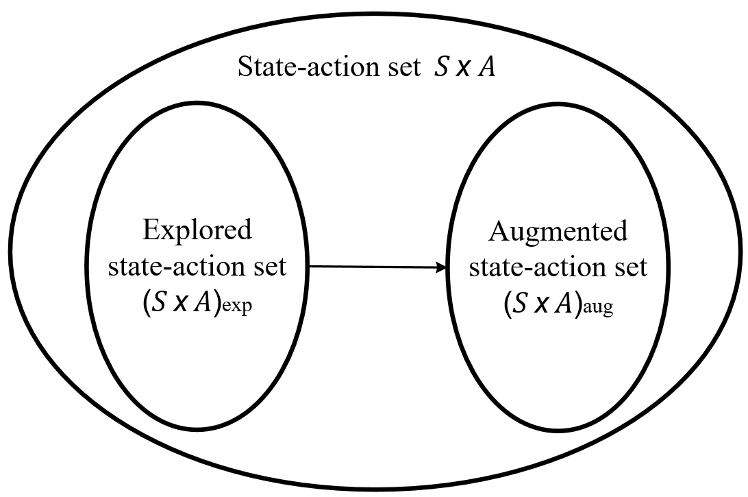
The discrete-time dynamical system in Eq.(1) is a symmetric dynamical system with respect to a reference point , when the following equations hold:
| (22) | ||||
where , are state space and action space of dynamical system (1). Figure 1 illustrates symmetry relation of state-action set in a dynamical system.
Definition 3. (Symmetric reward function)
For reward function defined in Eq.(2), it is symmetric with respect to state-action pairs and in state-action space when
| (23) |
Definition 4. (Symmetric state-action value function)
For state-action value function defined in Eq.(4), it is symmetric with respect to state-action pairs and in state-action space , when
| (24) |
IV DDPG with symmetric data augmenation
This section presents a symmetry-integrated RL algorithm, namely DDPG-SDA. The symmetric data augmentation (SDA) algorithm is firstly developed based on symmetry assumptions defined in Section III. Then symmetric data augmentation is combined with standard DDPG algorithm, leading to DDPG-SDA.
IV-A Symmetric Data Augmentation
| (25) |
where is explored sample, is augmented sample. The matrices and are given as
| (26) |
IV-B DDPG with Symmetric Data Augmentation
The standard Deep Deterministic Policy Gradient (DDPG) is an off-policy RL algorithm for progressive optimization of a critic network to approximate Q value function, and a deterministic actor network to approximate policy function[34]. The specific optimization method is approximate policy iteration in Section II.C. For a DDPG agent, explored samples are stored in a replay buffer denoted by , i.e. .
Based on this, we propose to store augmented samples by Eq.(25) in same replay buffer, i.e.
Then an enriched dataset is available for training critic and actor networks. When one training step is executed, a batch of mixed state transitions with and are sampled to calculate losses for critic/actor networks. The losses are further used to update critic/actor network weights by gradient descent algorithm.
Despite of unchanged RL algorithm framework, we name the integrated learning algorithm that enriches dataset with symmetric data augmentation for standard DDPG as DDPG-SDA, i.e. deep deterministic policy gradient with symmetric data augmentation (see pseudo code in Algorithm 1).
| Algorithm 1: DDPG-SDA Algorithm |
| 1: Hyperparameters: critic/actor learning rate , delay factor |
| batchsize , update step , discount factor |
| Ornstein–Uhlenbeck (OU) process parameters |
| 2: Initialization: critic network parameter set , actor network parameter |
| set , empty replay buffer |
| 3: Initialization: target critic network parameter set , |
| target actor network parameter set |
| 4: Repeat |
| 5: Observe state and select action |
| , |
| 6: Execute in the environment |
| 7: Observe next state , reward , and done signal that indicates |
| whether is terminal |
| 8: Store sample and in replay buffer |
| 9: Calculate symmetric sample using |
| 10: Store sample and in replay buffer |
| 11: If is terminal then |
| 12: reset environment state |
| 13: If training is true then |
| 14: for each update step do |
| 15: Randomly choose samples from to compose sample set |
| 16: Calculate target values of samples in with |
| 17: Update parameter set for one step using gradient: |
| 18: Update parameter set for one step using gradient: |
| 19: Update parameter sets with |
| 20: end for |
| 21: end if |
| 22: until convergence |
V DDPG with symmetric critic augmenation
This section presents the second symmetry-integrated RL algorithm, namely DDPG-SCA. Firstly, performance analysis is provided for previous DDPG-SDA. Two modifications for RL algorithm framework are proposed to exploit augmented samples, i.e. piecewise Q value function approximation and two-step approximate policy iteration. Finally, the innovative RL algorithm with modified framework (DDPG-SCA) is developed and compared with previous two RL algorithms.
V-A Drawback of DDPG-SDA
DDPG-SDA algorithm makes use of augmented samples by mixing them with explored samples in training procedure. However, this mixed sample batch slows down DDPG-SDA agent learning in explored dataset because of less explored samples in one sample batch. Increasing sample batchsize is one solution to accelerate learning but a large batchsize may conversely degrade learning performance.
V-B Q Value Function Approximation with Two Critics
In order to efficiently exploit enlarged dataset for training critic/actor networks, we propose to modify RL framework so that it enables separate storage and utilization of explored and augmented samples.
For this purpose, two individual replay buffers denoted by are used for one RL agent, i.e.
In one training step, two critic networks are trained according to samples from buffers and , respectively. Therefore, the actual Q value function is approximated by two critic networks
| (27) |
V-C Two-step Approximate Policy Iteration
The alternate training for two critic and one actor networks is achieved by two-step approximate policy iteration method, i.e.
Step 1 (Approximate policy iteration with samples in )
| (28) |
| (29) |
Step 2 (Approximate policy iteration with samples in )
| (30) |
| (31) |
In step 1, critic and actor networks , are updated by approximate policy iteration in Section II.C. with samples from . In step 2, critic and actor networks are updated by same iteration method with samples from . As a result, critic networks are separately trained with explored and augmented datasets, actor network is trained with overall dataset. Specific update procedure by gradient descent algorithm is seen in Appendix B.
V-D DDPG with Symmetric Critic Augmentation
On the basis of standard DDPG algorithm with enlarged dataset by symmetric data augmentation, the proposed modifications for RL framework in Section V.B&C. result into an innovative RL algorithm named as DDPG-SCA, i.e. deep deterministic policy gradient with symmetric critic augmentation. By using two critic networks, enlarged number of samples from explored dataset and augmented dataset are utilized in one training step so that training on overall dataset is accelerated. The pseudo code of DDPG-SCA is provided in algorithm 2.
| Algorithm 2: DDPG-SCA Algorithm |
| 1: Hyperparameters: critic/actor learning rate , delay factor |
| batchsize , update step , discount factor |
| Ornstein–Uhlenbeck (OU) process [35] parameters |
| 2: Initialization: critic network parameter sets , actor network |
| parameter set , empty replay buffers |
| 3: Initialization: target critic network parameter sets , |
| target actor network parameter sets |
| 4: Repeat |
| 5: Observe state and select action |
| , |
| 6: Execute in the environment |
| 7: Observe next state , reward , and done signal that indicates |
| whether is terminal |
| 8: Store sample and in replay buffer |
| 9: Calculate symmetric sample using |
| 10: Store sample and in replay buffer |
| 11: If is terminal then |
| 12: reset environment state |
| 13: If training is true then |
| 14: for each update step do |
| 15: Randomly choose samples from to compose sample set |
| 16: Calculate target values of samples in with |
| 17: Update parameter set for one step using gradient: |
| 18: Update parameter set for one step using gradient: |
| 19: Update parameter sets with |
| 20: Randomly choose samples from to compose sample set |
| 21: Calculate target values of samples in with |
| 22: Update parameter set for one step using gradient: |
| 23: Update parameter set for one step using gradient: |
| 24: Update parameter sets with |
| 25: end for |
| 26: end if |
| 27: until convergence |
VI Aircraft Model
This section introduces aircraft dynamical model in lateral plane. Firstly, a simplified linear model in continuous-time domain is presented for angular and angular rate variables. Then Euler method is used for model discretization. Lastly, Theorem 1 in Section III.A. is used to analyze symmetry property of state variables in discretized model.
VI-A Aircraft Linear Lateral Dynamics
The actual aircraft dynamics in lateral plane is nonlinear and time-varying with respect to flight conditions. To simplify process of model analysis, we use a linearized model which captures basic dynamic characteristics in lateral planes (see Ref.[36, 37]), i.e.
| (32) | ||||
where is bank angle, is roll rate, is sideslip angle, is yaw rate. is the deflection of aileron, is the deflection of rudder. Aerodynamic parameters are given in Table I.
VI-B Discretization
The lateral dynamical model in Eqs.(32) is discretized by one-order Euler method [38] with time step as
| (33) | ||||
The coefficient matrices , are given as
VI-C Symmetry Analysis
This subsection analyzes symmetry in aircraft lateral dynamics in Eq.(34) via Theorem 1. Theorem 1 categorizes symmetry planes into two cases: or , where second case requires enhanced constraint on system matrix . Coupling effects exist in Eq.(34) among increments of states from time step to and are included in .
Applying assumptions in Theorem 1 on system (34), one has
| (35) | ||||
where are state pairs symmetric to reference plane , are action pairs symmetric to .
VII Simulation Results
This section presents simulation results of developed RL algorithms by setting aircraft lateral model as environment. Training behaviors of are firstly compared to evaluate RL agents’s learning abilities. The tracking performances for untrained reference signal of RL-based lateral controllers are presented.
| Parameter | Value | Parameter | Value |
|---|---|---|---|
| -1.699 | 0 | ||
| 0.172 | 0.0488 | ||
| -4.546 | 0 | ||
| -0.0654 | -0.0829 | ||
| -0.0893 | 27.276 | ||
| 3.382m | 0.576 | ||
| 0 | 0.116 |
VII-A Online Training
Setting. Environment is set as aircraft lateral dynamics in Eqs. (32) implemented by Runge–Kutta fourth-order method with time step 0.1s. One episode of environment operation takes 300 time steps. Critic/Actor and target critic/actor network weights are initialized by Kaiming distribution in PyTorch linear module. Sampling from replay buffer is executed in a no-replacement way. Aircraft states are randomly initialized by uniform distributions, i.e. , , , . Actuator deflections are constrained as . The bank angle reference is a square-wave signal with period and amplitude , where is randomized at the beginning of each period by an uniform distribution . The shaping of reward considers tracking and stabilization, i.e. . To reduce unstable state transitions during training, angular rates and control efforts are used in reward to penalize aggressive changes of states, i.e.
| (37) | ||||
where . In Eq.(37), function is used to amplify tracking errors in set , and in set . is norm operator.
Baseline RL algorithm is selected as standard DDPG with same hyperparameters. Table II sets all hyperparameters.
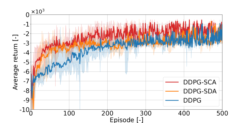
Training experiment for one RL algorithm consists of five instances with different random seeds. Each instance includes 3000 episodes of environment operation. To evaluate training performance, the metric ’average return’ is used and defined as mean of returns for 100 latest episodes.
| Parameter | Value |
|---|---|
| Critic learning rate | 0.001 |
| Actor learning rate | 0.001 |
| Delay factor | 0.01 |
| Discount factor | 0.99 |
| OU process parameters | 0.015,0.1,0.01 |
| Buffer size | 9106 |
| Batch size | 256 |
| Optimizer | Adam |
| Hidden layer structure | 6464 |
| Critic activation functions | ReLU |
| Actor output-layer activation function | tanh |
| Actor hidden-layers activation function | tanh-ReLU |
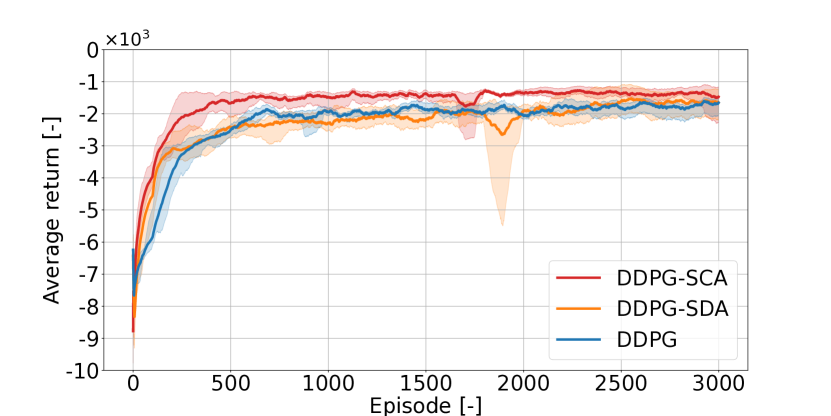
Results. Figure 2 provides ’average return’ histories of three RL algorithms for 500 episodes in training experiments. DDPG-SDA provides accelerated convergence to standard DDPG during first 200 episodes. This is because DDPG-SDA agent is additionally trained in symmetric state-action space in real-time even if this part of space is not explored by policy yet. DDPG-SCA shows improved acceleration to DDPG-SDA, which verifies that augmented samples are efficiently used by two-step policy iteration (see Section IV.C.). Furthermore, DDPG-SCA converges to largest ’average return’ steady value among three RL algorithms, verifying its ability to further optimize the actor network in 500 episodes. On the other hand, DDPG draws level with(flats) DDPG-SDA due to through exploration after 300 episodes. Converged training results for 3000 episodes are provided in Appendix C.
VII-B Online Operation
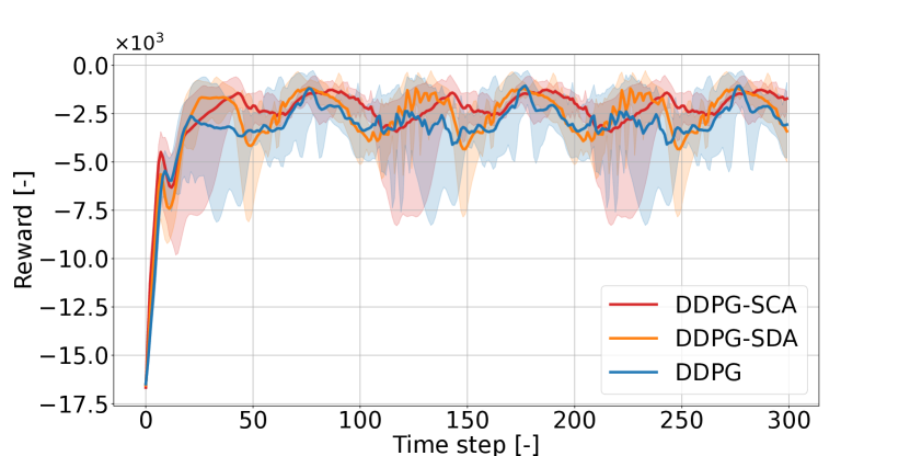
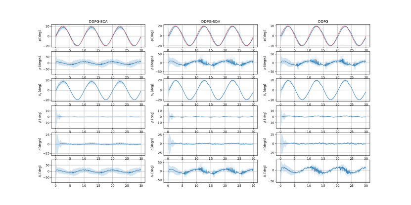
Setting. The reference is set as a sine-wave form as . Actor network weights are fixed after 3000-episode training. Initial aircraft states are randomized by same uniform distributions as in Section VI.A. The metric ’average reward’ in Figure 3 is an averaged value for rewards of each RL algorithm in same time step. Table III provides statistical results with mean and Standard Deviation(STD) of average reward for 30005 episode of environment operation for each RL algorithm.
| Metric/Algorithm | DDPG-SCA | DDPG-SDA | DDPG |
|---|---|---|---|
| Mean | -730.656 | -822.300 | -943.260 |
| Std | 253.942 | 101.244 | 182.641 |
VII-C Flight Controllers for Attitude Tracking
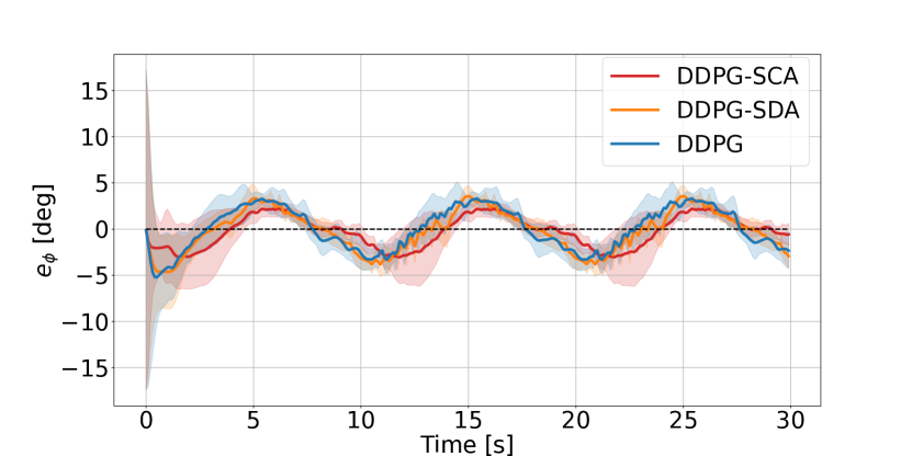
This subsection evaluates the tracking performances of flight controllers. The reference signals are set as . Tracking error and control effort are quatified with two metrics:
VII-C1 Tracking Error
The metric Integral of the Absolute Error Mean (IAEM) [39] is used to evaluate tracking error for trajectories with sequential horizon , which is calculated as . The auxiliary metric evaluates one trajectory with index .
VII-C2 Control Effort
Similar to the metric IAEM, we define Integral of the Absolute Control Mean (IACM) to evaluate control effort for trajectories, which is calculated as . The auxiliary metric evaluates control series for one trajectory with index .
| Channel | Metric | DDPG-SCA | DDPG-SDA | DDPG |
|---|---|---|---|---|
| Roll channel | IAEM | 1.044 | 1.136 | 1.225 |
| IACM | 54.630 | 21.898 | 19.649 | |
| Yaw channel | IAEM | 0.439 | 0.451 | 0.612 |
| IACM | 120.119 | 50.211 | 71.466 |
Table IV provides statistical results for three RL-trained controllers. Among three RL algorithms, DDPG-SCA trains a controller that achieves smallest values of IAEM in both roll channel and yaw channel. Meantime, DDPG-SCA controller consumes largest control effort through comparing IACM metric. These results indicate that DDPG-SCA provides an aggressive control policy.
By comparing results of DDPG-SDA and DDPG in Table IV, we observe that DDPG-SDA takes smaller control effort than DDPG to improve tracking error in yaw channel. In roll channel, DDPG-SDA achieves smaller tracking error with larger control effort than DDPG, indicating an aggressive tracking policy.
Figures 4 provides histories of tracking error by three controllers. Figure 5 shows histories of aircraft state variables and actuator deflections.
VIII Conclusion
This paper has presented two symmetry-integrated DDPG algorithms for exploiting augmented samples by symmetric data augmentation method. From the perspective of RL algorithm improvement, DDPG-SDA and DDPG-SCA are able to accelerate convergence in training phase, which reduce computation cost compared to standard DDPG. The resulting actor networks are able to provide satisfied generalization performance to untrained states. The fact accounting for the improvement is that symmetry-integrated RL algorithms capture symmetric motions of dynamical systems and make RL agents trained in an enlarged range of state-action space.
From an application perspective, symmetry-integrated RL algorithms match learning task of a class of physical systems with symmetry, e.g. aircraft lateral dynamics. Because symmetric samples are predicted instead of explored, the cost for getting these samples through interacting with actual systems is reduced. Therefore, symmetry-integrated RL algorithms show promising application potentials in real-world engineering field.
References
- [1] P.Zipfel, Aerodynamic Symmetry of Aircraft and Guided Missiles, Journal of Aircraft, vol.13, no.7, 1976.
- [2] Y.Yao, G.Xiong, K.Wang, et.al, Vehicle Detection Method based on Active Basis Model and Symmetry in ITS, IEEE Conference in Intelligent Transportation System(ITSC), The Hague, Netherlands, Oct, 2013.
- [3] F.Amadio, A.Colome, C.Torras, Exploiting Symmetries in Reinforcement Learning of Bimanual Robotic Tasks, IEEE Robotics and Automation Letters, vol.4, no.2, 2019, pp.1838-1845.
- [4] A.Mahajan, T.Tulabandhula, Symmetry Learning for Function Approximation in Reinforcement learning, 2017, arXiv:1706.02999.
- [5] Z.Martinot, Solutions to Ordinary Differential Equations using Methods of Symmetry, University of Washton, USA, 2014.
- [6] M.Weissenbacher, S,Sinha, A.Garg, Y.Kawahara, Koopman Q-learning: offline reinforcement learning via symmetries of dynamics, Proceedings of the 39th International Conference on Machine Learning(ICML), Baltimore, USA, Mar, July, 2022.
- [7] G.Russo, J.E.Slotine, Symmetries, Stability and Control in Nonlinear Systems and Networks, MIT, USA, 2014.
- [8] M.Zinkevich, T.Balch, Symmetry in Markov Decision Process and its Implications for Single Agent and Multiagent Learning, Proceedings of the 18th International Conference on Machine Learning, Massachusetts, USA, 2001.
- [9] E.van der Pol, D.Worrall, et.al, MDP Homomorphic Networks: Group Symmetries in Reinforcement Learning, Conference on Neural Information Processing Systems(NeurIPS), Vancouver, June, 2020.
- [10] S.Liu, M.Xu, P.Huang, X.Zhang, et.al, Continual vision-based reinforcement learning with group symmetries, 7th Conference on Robot Learning(CoRL), Atlanta, USA, November, 2015.
- [11] W.Yu, G.Turk and C.K.Liu, Learning symmetric and low-energy locomotion, ACM Transactions on Graphics, vol.(37), no.(4), 2018.
- [12] F.Abdolhosseini, H.Y.Ling, Z.Xie, et.al, On learning symmetric locomotion, Proceedings of 12th ACM Conference on Motion, Interaction and Games, Newcastle, U.k., October 2019.
- [13] M.Kasaei, M.Abreu, N.Lau, et.al, A CPB-based Agile and Versatile Locomotion Framework with Proximal Symmetry Loss Function, arXiv:2103.00928, 2021.
- [14] M.Abreu, L.P.Reis, N.Lau, Addressing Imperfect Symmetry: a Novel Symmetry-Learning Actor-Critic Extension, arXiv:2309.02711, 2023.
- [15] M.A.S.Kamal, J.Murata, Reinforcement learning for problems with symmetrical restricted states, Robotics and Autonomous Systems, vol.(56), 2008, pp.717-727.
- [16] S.Mishra, A.Abdolmaleki, A.Guez, et.al, Augmenting Learning Using Symmetry in a Biologically-inspired Domain, arXiv:1910.00528, 2019.
- [17] G.Angelotti, N.Drougard, and C.P.C.Chanel, Expert-guided Symmetry Detection in Markov Decision Process, ICAART, 2022.
- [18] G.Angelotti, N.Drougard, C.P.C.Chanel, Data Augmentation Through Expert-guided Symmetry Detection to Improve Performance in Offline Reinforcement Learning, International Conference on Agents and Artificial.
- [19] J.Brandstetter, M.Welling, D.E.Worral, Lie Point Symmetry Data Augmentation for Neural PDE Solvers, 2022.
- [20] R.Wang, R.Walters, and R.Yu. Incorporating symmetry into deep dynamics models for improved generalization. International Conference on Learning Representations(ICLR), 2021.
- [21] R.Wang, R.Walters, R.Yu, Data augmentation vs. equivariant networks: A theory of generalization on dynamics forecasting, ICML, 2022.
- [22] Y.Lin, J.Huang, et.al, Towards more sample efficiency in reinforcement learning with data augmentation, NIPS, 2019.
- [23] Y.Lin, J.Huang, M.Zimmer, et.al, Invariant transform experience replay: data augmentation for deep reinforcement learning, IEEE Transactions on Robotics and Automation Letters, vol.5, no.4, pp:6615-6622, 2020. Intelligence(ICAART), Lisbon, Portugal, 2023.
- [24] C.Pinneri, S.Bechtle, Equivariant Data Augmentation for Generalization in Offline Reinforcement Learning, ICML, 2023.
- [25] R.Wang, R.Walters, R.Yu, Approximately Equivariant Networks for Imperfectly Symmetric Dynamics, ICML, 2022.
- [26] J.Huang, W.Zeng, H.Xiong, et.al, Symmetry-informed Reinforcement Learning and its Application to Low-Level Attitude Control of Quadrotors, IEEE Transactions on Artificial Intelligence, vol(5), no.(3), pp: 1147-1161.
- [27] H.Han, J.Cheng, Z.Xi, B.Yao. Cascade Flight Control of Quadrotors Based on Deep Reinforcement Learning, IEEE Robotics and Automation Letters, 2022.
- [28] Y.ang, J.Sun, H.He, C.Sun. Deterministic Policy Gradient With Integral Compensator for Robust Quadrotor Control, IEEE Transactions on Systems, Man, and Cybernetics: Systems, 2020.
- [29] B.Ma. Z.Liu, Q.Dang, et.al. Deep Reinforcement Learning of UAV Tracking Control Under Wind Disturbances Environments, IEEE Transactions on Instrumentation and Measurement, 2023.
- [30] M.Chowdhury, S.Keshmiri, et.al. Interchangeable Reinforcement-Learning Flight Controller for Fixed-Wing UASs, IEEE Transactions on Aerospace and Electronic Systems, early access.
- [31] E.Bohn, E.M.Coates, D.Reinhardt, T.A.Johansen. Data-Efficient Deep Reinforcement Learning for Attitude Control of Fixed-Wing UAVs: Field Experiments, IEEE Transactions on Neural Networks and Learning Systems, 2024.
- [32] H.Jiang, H.Xiong, W.Zeng, et.al. Safely learn to Fly Aircraft From Human: An Offline–Online Reinforcement Learning Strategy and Its Application to Aircraft Stall Recovery, IEEE Transactions on Aerospace and Electronic Systems, vol(59), no.(6), pp: 8194-8207.
- [33] B.Ma. Z.Liu, W.Zhao, et.al. Target Tracking Control of UAV Through Deep Reinforcement Learning, IEEE Transactions on Intelligent Transportation Systems, 2023.
- [34] T.P.Lillicrap, J.J.Hunt, A.Pritizel, et.al, Continuous Control with Deep Reinforcement Learning, International Conference on Learning Representations (ICLR), 2016.
- [35] J.L.Doob, The Brownian Movement and Stochastic Equations, Annals of Mathematicals, Mathematics Department, Princeton University, 1942..
- [36] H.Ohta, P.N.Nikiforuk and M.M.Gupta, Design of Desirabale Handling Qualities for Aircraft Lateral Dynamics, Journal of Guidance, Control and Dynamics, vol.2, no.1, 1979, pp.31-39.
- [37] H.Ohta, P.N.Nikiforuk and M.M.Gupta, Some analytical control laws for the design of desirable lateral handing qualities using the model matching method, AIAA Paper 77-1045, Hollywood, Fla., Aug. 8-10, 1977.
- [38] H.J.Stetter, Analysis of discretization methods for ordinary differential equations, Springer,1973.
- [39] S.M.Shinner, Modern control system theory and application, Addison-Wesley, 2nd, 1978.
IX Appendix
IX-A Proof of Theorem 1
Theorem 1. (Symmetry of )
For a discrete-time system model (1), two state transition samples , and a reference point are selected. By assuming Eqs.(19), (20) hold, is a symmetric point for when following conditions hold:
(1)
(2) .
Proof.
Assume states are symmetric to the reference , i.e.
| (38) |
and are symmetric to 0, i.e.
| (39) |
The next-step state by taking actions at is derived by system model (1) as
| (40) |
The next-step state by taking actions at is derived by system model (1) as
| (41) |
If are symmetric to , the following equation holds
| (44) |
Rewrite (45) as
| (46) |
Eq.(46) is a general condition for symmetry of to .
In Eq.(46), the term 1, term 2 describe how the system function and control function affect the symmetry, when transfer to . If term 1 and term 2 both equal 0, it means that the symmetry of are same as that of . If term 1 and term 2 do not equal 0, it means that are not symmetric.
For convenience of further discussion, two cases are considered:
Case 1: .
From Eq.(38), one has
| (47) |
Substitute (47) into term 1:
| (48) | ||||
Because does not always hold, the condition that term 1 is identically 0 becomes .
Rewrite term 2 as
| (49) | ||||
Because does not always hold, the condition that term 2 is identically 0 becomes .
Case 2: .
From Eq.(38), one has
| (50) |
Substitute (50) to term 1:
| (51) | ||||
Because , the condition for Eq.(51) equals 0 is
| (52) | |||
The analysis of term 2 is similar to that in case 1.
Rewrite term 2 as
| (53) | ||||
Because does not always hold, the condition that term 2 is identically 0 becomes .
Q.E.D.
IX-B Implementation of two-step approximate policy iteration
Two-step approximate policy iteration is numerically implemented by gradient descent algorithm, to progressively optimize parameter sets , of used networks.
Step 1. (Approximate policy iteration with samples in )
Policy evaluation for critic :
Substitute one sample from buffer into Eq.(28):
| (54) |
Slowing down recursive updates of parameter set by Eq.(55) helps to stabilize learning process, which is implemented by introducing a target critic network and an actor network for right side of equation, i.e.
| (55) |
In Eq.(55), for known parameter set in th step, solving parameter set in th step analytically is difficult because of network nonlinearity. To address this issue, progressive optimization is used by gradient descent algorithm to minimize errors between left and right sides of Eq.(55).
Define the innovation error as
| (56) |
For a batch of samples denoted with from buffer , Mean Square Error (MSE) loss is calculated as
| (57) |
where is the number of samples, is index number for samples.
The gradient of loss with respect to parameter set is derived as
| (58) |
where
| (59) |
Then Eq.(58) is rewritten as
| (60) | ||||
Parameter set is updated using gradient descent method for one step as
| (61) |
The parameter set is updated by
| (62) |
Policy Improvement for actor by critic
The purpose of policy improvement is to find an action produced by actor that minimizes function .
Substitute a sample in into (29):
| (63) |
Solving Eq.(63) analytically is difficult because of network nonlinearity and complex function . For known parameter set in th step, an optimized parameters set can be calculated by gradient descent algorithm.
Define loss for one sample as
| (64) |
For a batch of samples from used in (57), the MSE loss is calculated by
| (65) |
where is number of samples in , is index number of one sample.
The gradient of loss with respect to parameter set is derived as
| (66) |
where
| (67) | ||||
Parameter set is updated using gradient descent method for one step as
| (68) |
Parameter set is updated by
| (69) |
where is a delay factor.
Step 2. (Approximate policy iteration with samples in )
Policy evaluation for critic :
Substitute one sample from buffer into Eq.(30):
| (70) |
To slow down updates of parameter sets by Eq.(70), a target critic network and a target actor network are introduced, i.e.
| (71) |
To solve parameter set with known in Eq.(71), progressive optimization is used by gradient descent algorithm to minimize errors between left and right sides of Eq.(71).
Define the innovation error as
| (72) |
For a batch of samples denoted with from buffer , Mean Square Error (MSE) loss is calculated as
| (73) |
where is the number of samples, is index number for samples.
The gradient of loss with respect to parameter set is derived as
| (74) |
where
| (75) |
Then Eq.(74) is rewritten as
| (76) | ||||
Parameter set is updated using gradient descent method for one step as
| (77) |
Parameter set is updated by
| (78) |
Policy Improvement for actor by critic
The purpose of policy improvement is to find an action produced by actor that minimizes function .
Substitute a sample in into (31):
| (79) |
Solving Eq.(79) analytically is difficult because of network nonlinearity and complex function . For known parameter set in th step, an optimized parameters set can be calculated by gradient descent algorithm.
Define loss for one sample as
| (80) |
For a batch of samples from used in (73), the MSE loss is calculated by
| (81) |
where is number of samples in , is index number of one sample.
The gradient of loss with respect to parameter set is derived as
| (82) |
where
| (83) | ||||
Parameter set is updated using gradient descent method for one step as
| (84) |
Parameter set is updated by
| (85) |
IX-C Additional training results
Figure 6 overviews average return for 3000-episode training experiments. Three RL algorithms converge to close final values, which indicates DDPG is capable of finding an optimized policy without taking advantage of augmented data.
To further evaluate learning performance, Table V provides statistical results of average return histories in ascent stage (0500 episodes) and setting stage (25003000 episodes). The metric ’average gradient’ quantifies convergence speed of average return. By comparing average gradients of DDPG-SDA (8.045) and DDPG (7.489), we conclude that symmetric data of a dynamical system averagely accelerates policy learning in overall ascent stage for a RL agent with unchanged hyperparameters and algorithm structure. By comparing average gradients of DDPG-SCA (14.212) and DDPG-SDA (8.045), we conclude that two-step approximate policy iteration in a RL algorithm makes better use of symmetric data than one-step approximate policy iteration does in terms of accelerating policy learning.
On the other hand, we observe that average return of standard DDPG overtakes that of DDPG-SDA after 500 episodes. This is explained by two reasons: (1) DDPG agent explores sufficient samples in symmetric state-action space with increased number of training episodes. (2) DDPG actor network generalizes its performance on unexplored state-action pairs in .
| Metric/Algorithm | DDPG-SCA | DDPG-SDA | DDPG |
|---|---|---|---|
| Average return (Ep.500) | -1672.669 250.239 | -2408.224 234.935 | -2499.168 147.257 |
| Average gradient (Ep.1-500) | 14.2122.118 | 8.0451.058 | 7.4892.805 |
| Average return (Ep.3000) | -1468.781 395.151 | -1643.008 345.124 | -1654.506 197.981 |
| Average gradient (Ep.2500-3000) | -0.1970.678 | -0.0560.212 | 0.3260.099 |