MonoSparse-CAM: Harnessing Monotonicity and Sparsity for Enhanced Tree Model Processing on CAMs

Abstract.

Despite significant advancements in AI driven by neural networks, tree-based machine learning (TBML) models excel on tabular data. These models exhibit promising energy efficiency, and high performance, particularly when accelerated on analog content-addressable memory (aCAM) arrays. However, optimizing their hardware deployment, especially in leveraging TBML model structure and aCAM circuitry, remains challenging.

In this paper, we introduce MonoSparse-CAM, a novel content-addressable memory (CAM) based computing optimization technique. MonoSparse-CAM efficiently leverages TBML model sparsity and CAM array circuits, enhancing processing performance. Our experiments show that MonoSparse-CAM reduces energy consumption by up to 28.56$\times$ compared to raw processing and 18.51$\times$ compared to existing deployment optimization techniques. Additionally, it consistently achieves at least 1.68$\times$ computational efficiency over current methods.

By enabling energy-efficient CAM-based computing while preserving performance regardless of the array sparsity, MonoSparse-CAM addresses the high energy consumption problem of CAM which hinders processing of large arrays. Our contributions are twofold: we propose MonoSparse-CAM as an effective deployment optimization solution for CAM-based computing, and we investigate the impact of TBML model structure on array sparsity. This work provides crucial insights for energy-efficient TBML on hardware, highlighting a significant advancement in sustainable AI technologies.

1. Introduction

Artificial intelligence (AI) has revolutionized numerous fields, including computer vision, robotics and health care (LeCun et al., 2015; Pedro et al., 2023; Bi et al., 2023). These accomplishments are fueled by deep neural network models trained on large datasets. However, tree-based models have shown superior performance on tabular data compared to their deep learning counterparts (Grinsztajn et al., 2022; Shwartz-Ziv and Armon, 2021; Gorishniy et al., 2021). Additionally, tree-based models are also more interpretable and easier to debug. For this reason, implementing tree-based models in hardware is a growing topic of research. One implementation of a tree-based model was realized by mapping a tree structure onto an analog content-addressable memory (aCAM) array (Pedretti et al., 2021).

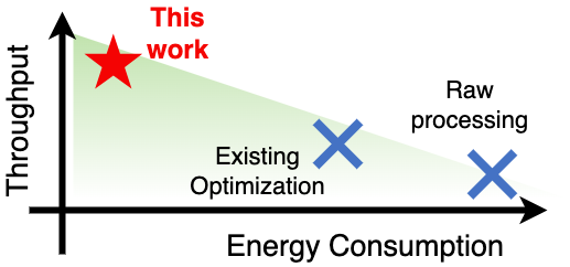
(a)

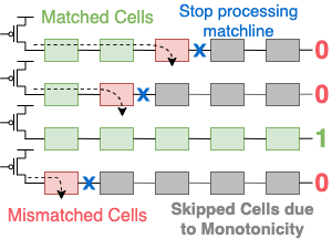
(b)

Figure 1. (a) Challenges in scalable CAM and (b) proposed MonoSparse-CAM architecture.

A comparison of TBML accelerators has been made in the literature, highlighting memristive analog CAMs as the least energy hungry option (Pedretti et al., 2021; Li et al., 2020). Architecture optimization of TBML accelerators is crucial for processing large arrays, which are difficult to fabricate. Prior works have explored different deployment management techniques to optimize the processing performance. Feature reordering (FR) is a novel approach in architecture optimization, prioritizing the reordering of rows and columns based on activity levels, effectively concentrating the most active cells towards the bottom left corner of the array (Pedretti et al., 2021). By prioritizing active cells and skipping empty ones, FR saves time and energy consumption, with a slight improvement in throughput as shown in Fig. 1(a). While the exact-matching technique has been widely used, other potentially efficient matching criteria, such as best match, threshold match, and partial match, have yet to be implemented in hardware (Hu et al., 2021).

This paper introduces and evaluates a software-hardware co-design for accelerating TBML models on CAMs, focusing on how model sparsity influences algorithm choice for optimizing CAM-based computation. This paper makes the following contributions:

• We present MonoSparse-CAM, a novel CAM-based computing optimization algorithm that leverages decision-tree sparsity and CAM array monotonicity.

• We explore how tree-based model shapes affect array sparsity, highlighting the need for a tree-aware technique.

• We demonstrate that MonoSparse-CAM effectively addresses scalability issues in large array processing and significantly reduces the high energy consumption inherent in CAM circuitry.

Our results show that the structural balance of a binary TBML model is an indicator of sparsity in the array, presenting opportunities for further optimization. Regardless of sparsity levels, by acknowledging the circuit’s monotonocity as shown in Fig. 1(b), a large array can be processed with minimal energy consumption whilst maintaining high accuracy and throughput. Compared to state-of-the-art (SOTA) technique, MonoSparse-CAM reduces energy consumption by 3.45$\times$ for high sparsity arrays and 18.51$\times$ for low sparsity arrays.

2. Background

2.1. Tree-Based Machine Learning (TBML) Models

A tree-based model is a machine learning approach that trains a decision tree to classify data based features. A feature vector is provided to a parent node and one feature is compared to upper and lower bounds. Depending on the outcome, the algorithm descends to either the right or left child node. This process continues until the final child node, where a logical True value classifies the data into the associated class. Fig. 2(a) shows an example of a decision tree for a dataset with four features and six terminating child nodes, each representing a final classification.

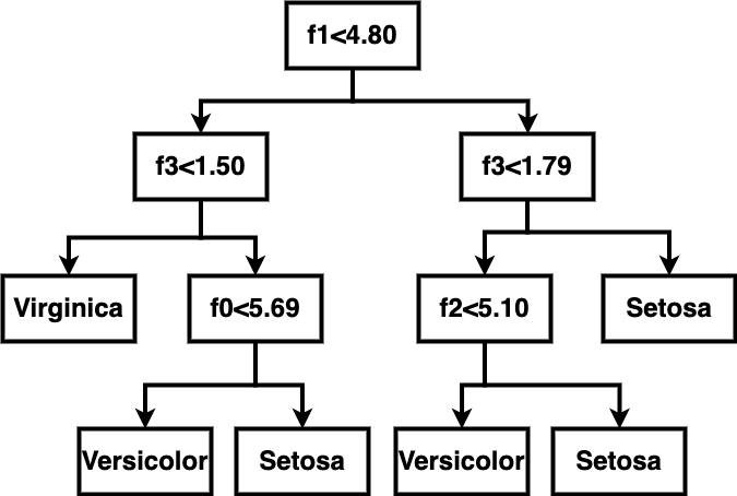
(a)

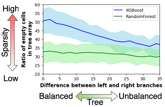
(b)

Figure 2. (a) A 4-feature XGBoost decision tree trained on the Iris Dataset (Fisher, 1988). (b)The effect of structural imbalance on tree sparsity shows that as binary trees become more balanced, they become more sparse.

In real-world applications, tabular data, which consists of samples with the same number of features, is one of the most common data types (Liu et al., 2022; Luo et al., 2020). Top performing TBML models, such as Random Forest and XGBoost, consist of ensembles of decision trees. These models are highly interpretable and transparent, which is crucial in fields requiring explainability. Due to their interpretability, cost effectiveness, and high performance, TBML algorithms remain SOTA for tabular data (Borisov et al., 2021).

With the success of deep learning on data types such as images, text, and audio, there has been a recent interest in using deep neural network (DNN) models for tabular data (Joseph, 2021; Zhu et al., 2021; Richman and Wüthrich, 2021). However, SOTA TBML models, such as XGBoost and RandomForest, consistently outperform deep learning models on diverse tabular datasets with the same tuning protocols (Grinsztajn et al., 2022; Shwartz-Ziv and Armon, 2021; Gorishniy et al., 2021). Additionally, in federated learning settings, TBML models still outperform federated DNNs on tabular data (Lindskog and Prehofer, 2023). Despite the high accuracy of DNNs, the computational workload required by training DNNs has a surprisingly large carbon footprint (Schwartz et al., 2020). In a recent study, TBML models were trained on real-world data to predict effluent pH and concentration in the capacitive deionization process. These ensemble models incurred 100$\times$ less computational cost than a DNN model whilst achieving the same level of accuracy (Ullah et al., 2023).

2.2. Sparsity in Tree-Based Models

Tree-based models’ structures, which can vary in balance and sparsity based on their training, significantly influence decision-making processes. Balance refers to the difference in the number of nodes between the left and right sub-trees splitting from the root node; a balanced tree has nearly equal nodes in both sub-trees. Tree-based models, depending on their training, can suffer from sparsity. Investigating the correlation between the architecture of decision trees and their performance is essential, including the impact of tree balance, sparsity, and their representations in data processing. For instance, a tree’s structure, particularly its sparsity and balance, can affect the performance of different CAM-based computing optimization algorithms. Sparse tree structures may favor specific algorithms, leading to higher computational efficiency. Understanding these nuances is crucial for optimizing decision tree performance in various applications. While an earlier technique has sped up processing, it comes with notable limitations. Specifically, FR excels with sparse trees but falls short with less sparse trees.

2.3. Analog CAM Arrays

CAM cells were originally designed to quickly find the location of data in memory based on the desired input contents. In digital CAM, cells are connected horizontally by match-lines (MLs) and vertically by data-lines (DLs). Before a search, MLs are pre-charged to a high logic state, and the desired bit sequence is provided to the DLs. A mismatch between the bit stored in the CAM cell and the bit on the DL discharges the matchline. At the end of the search, any ML that is not discharged corresponds to a match in that row. Analog CAM cells work similarly, but check if the provided analog voltage on the DL falls within a range between lower bound and upper bound voltages. One implementation of an analog CAM cell (Li et al., 2020) uses memristors in common-source amplifiers to compare the input voltage to a threshold and activate an NMOS to discharge the ML. Memristors are two-terminal devices with tunable, nonvolatile resistances (Chua, 1971), allowing the threshold of the cell to be changed. Fig. 3(d) shows a diagram of this circuit. An analog CAM cell stores ranges from 0 to 1 using its lower-bound and upper-bound subcircuits. An empty, or ”don’t care”, cell is stored by setting the low bound to 0 and the high bound to 1, outputting a ”match” to any input.

Previous works have used analog CAMs to implement TBML models efficiently (Pedretti et al., 2021). When mapping a model to a CAM array, each row represents a complete path through the tree, from the root node to a final terminating child node that represents a classification. Paths through the tree can be rearranged such that each column includes all nodes for a given feature of the data. The feature is converted into a voltage and applied to the DL, and any matching MLs indicate the data belongs to the associated class. As the order of the features is arbitrary in each root-to-leaf path, FR reorders the features (columns) based on occurrence, moving all active or important features to the left side of the array. Similarly, rows are reordered based on the number of non ”empty” cells, moving the most populated rows to the bottom of the array. This leaves the top right region of the array largely empty, offering compressibility and efficient tiling of a large data array onto reasonably-sized analog CAM arrays (Pedretti et al., 2021).

2.4. High Power Consumption in CAMs

Content Addressable Memory (CAM) is renowned for its rapid data retrieval but struggles with high power consumption due to simultaneous activation of large chip portions (Do et al., 2013). This limits scalability in power-constrained environments. Addressing this at both the inter-array circuitry and architectural levels, recent advances include novel TCAM cell circuits with memristor devices (Graves et al., 2022) and hybrid-type CAM designs that balance NOR-type CAM’s speed with NAND-type CAM’s energy efficiency (Choi et al., 2005). NOR-type CAMs use precharge/discharge for fast searches, while NAND-type CAMs use pass transistors for low-power, sequential searches. Additionally, architectural innovations like Feature Reordering have been developed (Pedretti et al., 2021). In this work, we focus on a method that merges characteristics from both levels, aiming for energy-efficient and high-speed processing.

3. Methodology

3.1. MonoSparse-CAM Algorithm

The MonoSparse-CAM algorithm builds upon FR by disabling processing for any row that has already received a mismatch. This method skips two kinds of cells: rows of empty cells and cells on an already discharged matchline. An empty, or “don’t care” cell, has a range of 0 to 1 and will match with any input value. If a row of all empty cells exists, we skip writing this row onto the aCAM array, as it will always get a row match.

Pre-charging the matchline before the computation cycle ensures monotonicity: once discharged, a matchline will not be pulled up again until the next pre-charge cycle. Any cell attempting to discharge an already discharged ML has no impact on the result of the circuit, as it is already a mismatch. This observation can be used to improve system efficiency. By leveraging the monotonicity of the CAM array, we propose a highly efficient CAM-based computing optimization algorithm, whose performance is unaffected by array sparsity.

Fig. 3(e) illustrates the use of a 2x2 analog CAM array to process a 10x6 model array, divided into three feature groups (fg0, fg1, fg2) to optimize the CAM’s width. This figure emphasizes a strategic data processing methodology where cells are selectively loaded onto the CAM based on criteria such as emptiness, discharge status, and monotonicity. By employing a tiling technique, a large decision-tree model’s array is divided into manageable segments that fit into the smaller physical CAM arrays (Pedretti et al., 2021). In the initial cycle (fg0), shown in purple outlining, selective loading is used to omit non-essential rows, indicated by light purple boxes with Xs. For example, rows ML8 and ML10 in fg0, ML10 in fg1, and ML4 in fg2 are skipped, and not loaded onto and procssed on CAMs, as these rows will automatically match the input. As demonstrated in Fig. 3(e), after the first cycle, rows ML2, ML5, ML6, and ML9 are deactivated, preventing any cells on these rows from being loaded onto the CAM in subsequent cycles. Following the second cycle, rows ML1, ML3, ML7, and ML8 are discharged, ensuring that cells on these rows are not loaded into the CAM in future cycles.

To keep track of the discharged matchlines, a register is needed. This register is updated after a feature group (i.e. FG0, FG1, FG2, …) is tiled, processed on aCAM, and ML states are retrieved. The register is accessed when the algorithm tiles the feature group and determines which rows to write onto the CAM.

To simulate large arrays with different levels of sparsity, we sample cells from a random Gaussian distribution, concentrating active cells near the center; according to previous studies, when an image is saved to an array, the most importance features are near the center while the least significant features are located around the edges (Pedretti et al., 2021). We use $\lambda$ values from 0.0 (low sparsity) to 1.0 (highly sparse), where $\lambda$ = 1.0 - $\sigma$, with $\sigma$ being standard deviation from the Gaussian distribution. Inputs to the tree or the large array are randomly generated and broken into arrays with length of $W_{VDL}/W_{CAM}$ each, with each fed into its corresponding feature group.

3.2. Sparsity Considerations and Tradeoffs

To explore the relationship between sparsity and structural balance in TBML models, we conducted an experimental analysis. Structurally-balanced trees reduce the computational complexity, allowing for faster computation and lower memory usage (Lundberg et al., 2020). We created binary classification datasets (1000 samples, 5 features), split them 67:33 for training and testing, and trained XGBoost and RandomForest models with a single decision tree (max depth 10). Structural balance was evaluated by calculating the difference in node counts between the left and right sub-trees. The trees were converted into arrays, and empty cells were counted. Repeating this 5000 times, we found an inverse relationship between tree balance and sparsity. XGBoost models has a Pearson Correlation coefficient of -0.35 (p-value 1.433E-148), and RandomForest models had a correlation of -0.327 (p-value 2.809E-125). These results indicate that well-balanced trees exhibit a high sparsity when mapped to arrays (Fig.  2(b)). Given the structural and sparsity differences among trees, an optimization technique capable of handling all types of TBML models is essential for efficient aCAM processing.

Fig. 4(a) shows that computation cost remains low for MonoSparse-CAM even in low sparsity scenarios (i.e., $\lambda$=0.5) where FR performs poorly. This is due to the increased number of non-empty cells, allowing the algorithm to leverage monotonicity more effectively. A higher number of non-empty cells increases the chances of encountering cells that predictably discharge the ML, enabling the algorithm to skip these computations and reduce overall computational cost. At lower sparsity levels, computational savings in MonoSparse-CAM are driven by monotonicity-based skipping, while at higher sparsity levels, savings come from Feature Reordering; as shown in Fig.4(a) and Fig.4(b), monotonicity-only techniques excel at low sparsity and Feature Reordering at high sparsity.

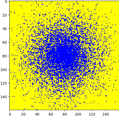
(a)

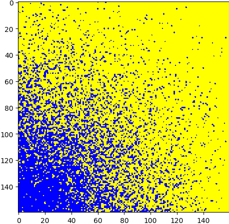
(b)

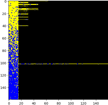
(c)

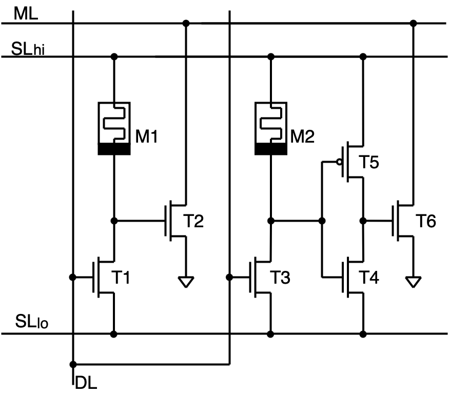
(d)

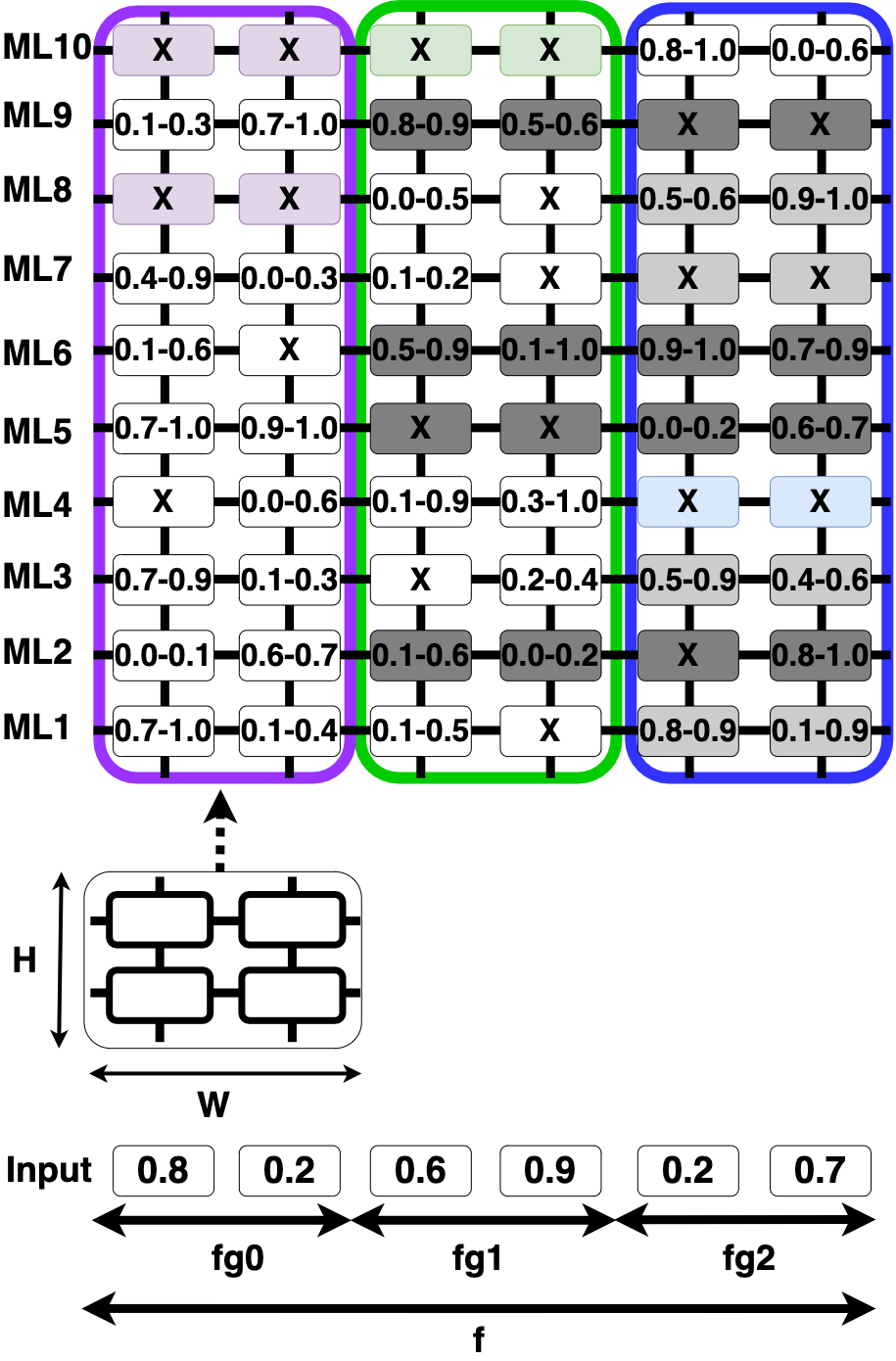
(e)

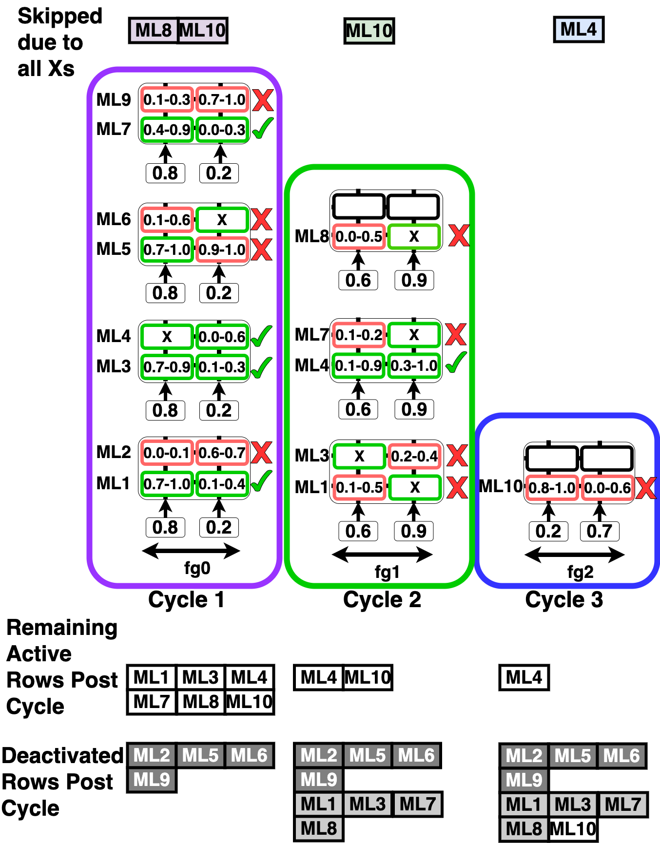
(f)

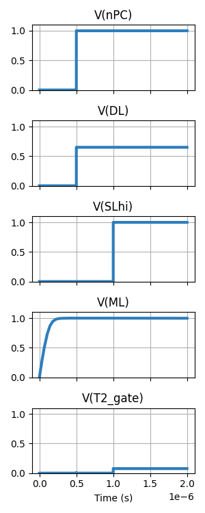
(g)

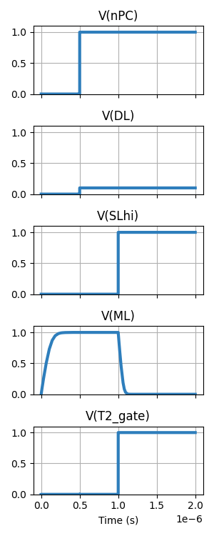
(h)

Figure 3. (a) A 160x160 array, representing a decision tree with 160 features and 160 terminating children nodes, simulated using a Gaussian distribution ($\lambda$ = 0.6, $\mu$ = 0.0). Yellow cells are empty and blue cells are non-empty. (b) The array after reordering features. (c) The array after the MonoSparse-CAM algorithm. Black cells are discharged due to monotonicity, saving computation and energy. (d) A schematic of a memristor-based analog CAM cell (Li et al., 2020). (e) Monotonicity-aware tiling: A 10x6 array processed using a 2x2 CAM. ”X” cells are empty cells. All X feature group rows are skipped. Dark/light grey cells are discharged by FG0/FG1. (f) Processing of each feature group processing. (g)-(h) A unit CAM cell’s match and mismatch operations, respectively.

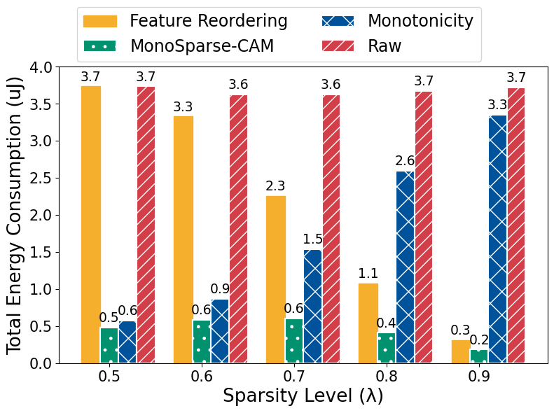
(a)

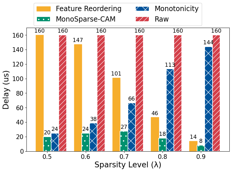
(b)

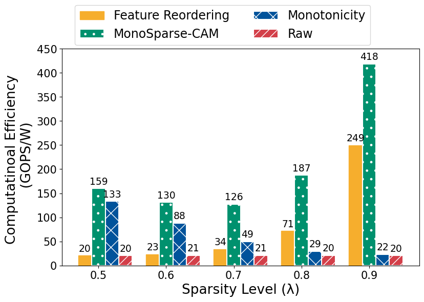
(c)

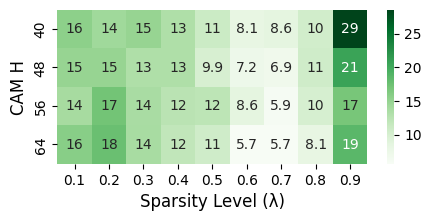
(d)

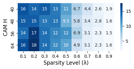
(e)

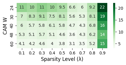
(f)

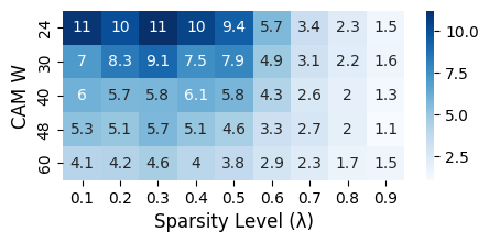
(g)

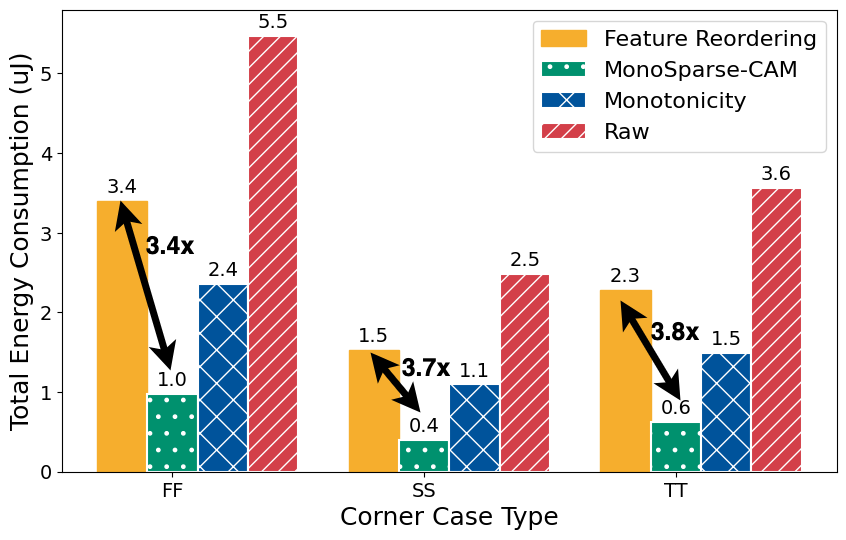
(h)

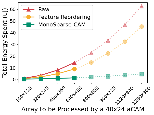
(i)

Figure 4. Comparison of (a) total energy consumption, (b) delay, and (c) computational efficiency between different optimization techniques when processing a 240x320 array with a 24x48 CAM. Gains of the MonoSparse-CAM over raw processing and FR are shown in green and blue for (d) and (e) width (W) = 16 with various heights and (f) and (g) height (H) = 48 with various widths, respectively. (h) Energy consumption comparison for processing a 240x320 array with a 24x48 CAM at $\lambda$=0.7 across different tech nodes: typical (tt), slow NMOS and PMOS (ss), and fast NMOS and PMOS (ff). (i) Energy consumption projection: dotted lines show the predicted curve based on four actual data points connected by solid lines, with all fitted curves having an ${R}^{2}$ value above 97%.

3.3. Energy Consumption and Gain

Results for varying CAM widths differ from varying heights. A 320x240 array was processed using CAM arrays of varying heights (H=40 to 64, W=16) and varying widths (H=48, W=24 to 60) as shown in Fig. 4(d) and  4(e) and Fig. 4(f) and  4(g). Energy gain using the proposed algorithm over raw and FR processing is computed across different sparsity levels (green for raw in Fig. 4(d) and  4(f); blue for FR in Fig. 4(e) and  4(g)). Gain over FR, for instance, is computed as $\sum Energy_{FR}/\sum Energy_{MonoSparse-CAM}$. Results in Fig. 4 are averaged over at least three trials and Energy consumption measurements from Sense Amplifier were excluded. With a constant size of 24x48, total energy and delay for $\lambda$ values from 0.1 to 0.5 are the same as at $\lambda$=0.5. Therefore, Fig. 4a-c focus on $\lambda$ values from 0.5 to 0.9.

3.4. Circuit Simulation for analog CAM Cell and Arrays

The 6T2M analog CAM cells were designed in Cadence Virtuoso, with energy measurements simulated in HSPICE using the TSMC 65 nm PDK. A custom Python script varied CAM dimensions, configuring cell conductances and input voltages, with an 11 pF capacitor for each match line. Simulations used CMOS device models (TT, SS, FF). A specialized function linked voltage ranges to conductances, ensuring precise conductance-voltage relationships.

Fig.  3(g) shows a CAM cell match operation with conductance settings of 21.3 $\mu$S (lower bound) and 180.2 $\mu$S (upper bound). These settings kept the match line (ML) high for input voltages between 0.5V and 0.8V, demonstrating a succesful match with 0.65V. Conversely, Fig. 3(h) shows a mismatch operation with the same CAM cell and an input voltage of 0.1V, illustrating how variations in input voltage affect match outcomes.

4. Results and Discussion

We evaluate MonoSparse-CAM performance against existing methods by examining energy consumption, delay, and computation efficiency. We also assess how CAM size and process variations impact energy gain. Lastly, we address the high energy consumption of CAMs, which bottlenecks large array processing, and how MonoSparse-CAM mitigates this issue.

4.1. Energy Consumption and Delay Analysis

A 240x320 array is processed using a 24x48 CAM. Fig. 4(a) shows that, for raw processing, the total energy consumption stays stable across different sparsity levels (mean = 3.77$\mu$J, stdev = 0.15$\mu$J). FR achieves 15$\times$ energy gain at high sparsity ($\lambda$ = 0.9), but its energy usage increases at lower sparsity, matching raw processing levels. MonoSparse-CAM consistently achieves the lowest total energy consumption across all sparsity levels (mean = 0.40$\mu$J, stdev = 0.48$\mu$J), with energy gains peaking at 22.16$\times$ over raw processing and 10.96$\times$ over FR.

4.2. Size Variability Analysis

The width and height of a CAM array significantly impact total energy consumption. Fig. 4(e) and 4(d) demonstrate that smaller heights often yield the highest gains, with high sparsity arrays reaching up to 28.56× gain over raw and 2.00× over FR, and low sparsity arrays achieving up to 18.51× over both. Varying CAM widths show similar patterns, with high sparsity arrays reaching up to 22.17× over raw and 3.45× over FR, and low sparsity arrays achieving up to 11.0× over both.

Gain varies more with changes in width than changes in height. Reduced width improves energy efficiency because the system’s register can quickly identify discharged MLs, skipping them in the subsequent feature group cycle and streamlining computation. For instance, in a 160-cell wide array, if a mismatch occurs at cell 80 and is processed by CAM arrays with a width of 8, the algorithm stops after 10 operations, checking 80 cells. Processed by CAM arrays with a width of 32, the algorithm stops after 3 operations, checking 96 cells, 16 more than necessary.

(1) $$\text{GOPS/W}=\frac{H_{LargeArray}\cdot W_{LargeArray}/\text{Delay}_{Technique}}{\text{AvgPower}_{Technique}}$$

4.3. Computational Efficiency and Throughput Analysis

Fig. 4(c) presents the computational efficiency of different methods at varying sparsity levels, measured in Giga Operations Per Second per Watt (GOPS/W). MonoSparse-CAM consistently shows the highest computational efficiency, peaking at 418 GOPS/W (computed as in Eq. 1) for high sparsity ($\lambda$ = 0.9), while Feature Reordering shows moderate efficiency, and raw processing and monotonicity only processing exhibit lower efficiencies. These results highlight the significant performance gains of MonoSparse-CAM in optimizing computational efficiency across varying degrees of sparsity.

4.4. Corner Analysis

We explored the impact of corner analysis on different designs by examining three corners: TT (typical conditions), FF (fast NMOS, fast PMOS), and SS (slow NMOS, slow PMOS). Our simulations revealed significant variations in total energy consumption (µJ) across these corners, as illustrated in Fig. 4(h). MonoSparse-CAM consistently achieved the lowest total energy consumption across all corners, with at least 3.7x energy savings compared to existing methods.

4.5. Scalability Analysis

In Fig. 4(i), an array of increasing sizes (i.e., 160x120, 320x240, 480x360, 640x480) is processed by a 40x24 analog CAM using different techniques at $\lambda=0.7$ sparsity level. Prediction curves (with ${R}^{2}$ ¿ 0.97) are generated. As array size increases, energy usage grows exponentially with raw and FR, while MonoSparse-CAM shows nearly linear growth.

5. Conclusion

In this study, we introduced MonoSparse-CAM, a monotonicity and sparsity-aware technique for processing tree-based machine learning models with Content-Addressable Memory (CAM) arrays. This hardware-software co-designed approach successfully exploits the sparsity in tree-based models and the monotonicity of CAM circuits, leading to significant improvements in processing efficiency and energy consumption. Our method demonstrated a remarkable 28.56$\times$ and 18.51$\times$ reduction in energy consumption over raw processing and a state of the art optimization technique, respectively. These findings not only represent a major advancement in energy-efficient machine learning computation, but also set the stage for further innovations in the field, especially in the development of sustainable and resource-efficient machine learning architectures.

References

- (1)
- Bi et al. (2023) Ying Bi, Bing Xue, Pablo Mesejo, Stefano Cagnoni, and Mengjie Zhang. 2023. A Survey on Evolutionary Computation for Computer Vision and Image Analysis: Past, Present, and Future Trends. http://slubdd.de/katalog?TN_libero_mab2
- Borisov et al. (2021) Vadim Borisov, Tobias Leemann, Kathrin Seßler, Johannes Haug, Martin Pawelczyk, and Gjergji Kasneci. 2021. Deep Neural Networks and Tabular Data: A Survey.
- Choi et al. (2005) Sungdae Choi, K. Sohn, and Hoi-Jun Yoo. 2005. A 0.7-fJ/bit/search 2.2-ns search time hybrid-type TCAM architecture. IEEE Journal of Solid-State Circuits 40, 1 (2005), 254–260. https://doi.org/10.1109/JSSC.2004.837979
- Chua (1971) L. Chua. 1971. Memristor-The missing circuit element. IEEE Transactions on Circuit Theory 18, 5 (1971), 507–519. https://doi.org/10.1109/TCT.1971.1083337
- Do et al. (2013) Anh-Tuan Do, Shoushun Chen, Zhi-Hui Kong, and Kiat Seng Yeo. 2013. A High Speed Low Power CAM With a Parity Bit and Power-Gated ML Sensing. IEEE Transactions on Very Large Scale Integration (VLSI) Systems 21, 1 (2013), 151–156. https://doi.org/10.1109/TVLSI.2011.2178276
- Fisher (1988) R. A. Fisher. 1988. Iris. UCI Machine Learning Repository. DOI: https://doi.org/10.24432/C56C76.
- Gorishniy et al. (2021) Yury Gorishniy, Ivan Rubachev, Valentin Khrulkov, and Artem Babenko. 2021. Revisiting Deep Learning Models for Tabular Data. In Advances in Neural Information Processing Systems, M. Ranzato, A. Beygelzimer, Y. Dauphin, P.S. Liang, and J. Wortman Vaughan (Eds.), Vol. 34. Curran Associates, Inc., 18932–18943. https://proceedings.neurips.cc/paper_files/paper/2021/file/9d86d83f925f2149e9edb0ac3b49229c-Paper.pdf
- Graves et al. (2022) Catherine Graves, Can Li, Giacomo Pedretti, and John Paul Strachan. 2022. In-Memory Computing with Non-volatile Memristor CAM Circuits. Memristor Computing Systems, 105–139. https://doi.org/10.1007/978-3-030-90582-8_6
- Grinsztajn et al. (2022) Léo Grinsztajn, Edouard Oyallon, and Gaël Varoquaux. 2022. Why do tree-based models still outperform deep learning on tabular data? arXiv:2207.08815 [cs.LG]
- Hu et al. (2021) Xiaobo Hu, Michael Niemier, Arman Kazemi, Ann Franchesca Laguna, Kai Ni, Ramin Rajaei, Mohammad Sharifi, and Xunzhao Yin. 2021. In-Memory Computing with Associative Memories: A Cross-Layer Perspective. 25.2.1–25.2.4. https://doi.org/10.1109/IEDM19574.2021.9720562
- Joseph (2021) Manu Joseph. 2021. PyTorch Tabular: A Framework for Deep Learning with Tabular Data. arXiv:2104.13638 [cs.LG]
- LeCun et al. (2015) Yann LeCun, Yoshua Bengio, and Geoffrey Hinton. 2015. Deep learning. Nature 521, 7553 (01 May 2015), 436–444. https://doi.org/10.1038/nature14539
- Li et al. (2020) Can Li, Catherine E. Graves, Xia Sheng, Darrin Miller, Martin Foltin, Giacomo Pedretti, and John Paul Strachan. 2020. Analog content-addressable memories with memristors. Nature Communications 11, 1 (02 Apr 2020), 1638. https://doi.org/10.1038/s41467-020-15254-4
- Lindskog and Prehofer (2023) William Lindskog and Christian Prehofer. 2023. A Federated Learning Benchmark on Tabular Data: Comparing Tree-Based Models and Neural Networks. In Eighth International Conference on Fog and Mobile Edge Computing, FMEC 2023, Tartu, Estonia, September 18-20, 2023. IEEE, 239–246. https://doi.org/10.1109/FMEC59375.2023.10305887
- Liu et al. (2022) Dugang Liu, Pengxiang Cheng, Hong Zhu, Xing Tang, Yanyu Chen, Xiaoting Wang, Weike Pan, Zhong Ming, and Xiuqiang He. 2022. DIWIFT: Discovering Instance-wise Influential Features for Tabular Data. Proceedings of the ACM Web Conference 2023 (2022). https://api.semanticscholar.org/CorpusID:250311631
- Lundberg et al. (2020) Scott M. Lundberg, Gabriel Erion, Hugh Chen, Alex DeGrave, Jordan M. Prutkin, Bala Nair, Ronit Katz, Jonathan Himmelfarb, Nisha Bansal, and Su-In Lee. 2020. From local explanations to global understanding with explainable AI for trees. Nature Machine Intelligence 2, 1 (01 Jan 2020), 56–67. https://doi.org/10.1038/s42256-019-0138-9
- Luo et al. (2020) Yuanfei Luo, Hao Zhou, Wei-Wei Tu, Yuqiang Chen, Wenyuan Dai, and Qiang Yang. 2020. Network On Network for Tabular Data Classification in Real-world Applications. Proceedings of the 43rd International ACM SIGIR Conference on Research and Development in Information Retrieval (2020). https://api.semanticscholar.org/CorpusID:218719316
- Pedretti et al. (2021) Giacomo Pedretti, Catherine E. Graves, Sergey Serebryakov, Ruibin Mao, Xia Sheng, Martin Foltin, Can Li, and John Paul Strachan. 2021. Tree-based machine learning performed in-memory with memristive analog CAM. Nature Communications 12, 1 (04 Oct 2021), 5806. https://doi.org/10.1038/s41467-021-25873-0
- Pedro et al. (2023) Ana Rita Pedro, Michelle B. Dias, Liliana Laranjo, Ana Soraia Cunha, and João V. Cordeiro. 2023. Artificial intelligence in medicine: A comprehensive survey of medical doctor’s perspectives in Portugal. PLOS ONE 18, 9 (09 2023), 1–24. https://doi.org/10.1371/journal.pone.0290613
- Richman and Wüthrich (2021) Ronald Richman and Mario V. Wüthrich. 2021. LocalGLMnet: interpretable deep learning for tabular data. arXiv:2107.11059 [cs.LG]
- Schwartz et al. (2020) Roy Schwartz, Jesse Dodge, Noah A. Smith, and Oren Etzioni. 2020. Green AI. Commun. ACM 63, 12 (nov 2020), 54–63. https://doi.org/10.1145/3381831
- Shwartz-Ziv and Armon (2021) Ravid Shwartz-Ziv and Amitai Armon. 2021. Tabular Data: Deep Learning is Not All You Need. In 8th ICML Workshop on Automated Machine Learning (AutoML). https://openreview.net/forum?id=vdgtepS1pV
- Ullah et al. (2023) Zahid Ullah, Nakyung Yoon, Bethwel Kipchirchir Tarus, Sanghun Park, and Moon Son. 2023. Comparison of tree-based model with deep learning model in predicting effluent pH and concentration by capacitive deionization. Desalination 558 (2023), 116614. https://doi.org/10.1016/j.desal.2023.116614
- Zhu et al. (2021) Yitan Zhu, Thomas Brettin, Fangfang Xia, Alexander Partin, Maulik Shukla, Hyunseung Yoo, Yvonne A. Evrard, James H. Doroshow, and Rick L. Stevens. 2021. Converting tabular data into images for deep learning with convolutional neural networks. Scientific Reports 11, 1 (31 May 2021), 11325. https://doi.org/10.1038/s41598-021-90923-y