Convergence analysis of the parareal algorithms for stochastic Maxwell equations driven by additive noise

Abstract

In this paper, we investigate the strong convergence analysis of parareal algorithms for stochastic Maxwell equations with the damping term driven by additive noise. The proposed parareal algorithms proceed as two-level temporal parallelizable integrators with the stochastic exponential integrator as the coarse $\mathcal{G}$-propagator and both the exact solution integrator and the stochastic exponential integrator as the fine $\mathcal{F}$-propagator. It is proved that the convergence order of the proposed algorithms linearly depends on the iteration number $k$. Numerical experiments are performed to illustrate the convergence order of the algorithms for different choices of the iteration number $k$, the damping coefficient $\sigma$ and the scale of noise $\lambda$.

Key Words: Stochastic Maxwell equations, Parareal algorithm, Strong convergence, Stochastic exponential integrator

1 Introduction

When the electric and magnetic fluxes are perturbed by noise, the uncertainty and stochasticity can have a subtle but profound influence on the evolution of complex dynamical systems [25]. In order to model the thermal motion of electrically charged microparticles, we consider the stochastic Maxwell equations with damping term driven by additive noise as follows

$$\left\{\begin{array}[]{ll}\varepsilon\partial_{t}\bm{E}(t,\bm{x})=\nabla\times\bm{H}(t,\bm{x})-\sigma\bm{E}(t,\bm{x})-J_{e}(t,x,\bm{E},\bm{H})-J_{e}^{r}(t,\bm{x})\cdot\dot{W},&(t,\bm{x})\in\left(0,T\right]\times D,\\ \mu\partial_{t}\bm{H}(t,\bm{x})=-\nabla\times\bm{E}(t,\bm{x})-\sigma\bm{H}(t,\bm{x})-J_{m}(t,x,\bm{E},\bm{H})-J_{m}^{r}(t,\bm{x})\cdot\dot{W},&(t,\bm{x})\in\left(0,T\right]\times D,\\ \bm{E}(0,\bm{x})=\bm{E}_{0}(\bm{x}),\bm{H}(0,\bm{x})=\bm{H}_{0}(\bm{x}),&\bm{x}\in D,\\ \bm{n}\times\bm{E}=0,&(t,\bm{x})\in\left(0,T\right]\times\partial D,\end{array}\right.$$ (5)

where $D\subset\mathbb{R}^{3}$ is an open, bounded and Lipschitz domain with boundary $\partial D$, of which $\bm{n}$ is the unit outward. Here $\varepsilon$ is the electric permittivity and $\mu$ is the magnetic permeability. The damping terms $\sigma\bm{E}$ and $\sigma\bm{H}$ are usually added to simulate the attenuation of electromagnetic waves in the medium, which can be caused by absorption, scattering or other non-ideal factors in the medium. The function $J_{e}$ and $J_{e}^{r}$ describe electric currents (or $J_{m}$ and $J_{m}^{r}$ describe magnetic currents). In particular, $J_{e}^{r}$ and $J_{m}^{r}$ do not depend on the electromagnetic fields $\bm{E}$ and $\bm{H}$. The authors in [22] proved the mild, strong and classical well-posedness for the Cauchy problem of stochastic Maxwell equations. Meanwhile, the authors in [20] studied the approximate controllability of the stochastic Maxwell equations via an abstract approach and a constructive approach using a generalization of the Hilbert uniqueness method. Subsequently the work [24] combined the study of well-posedness, homogenization and controllability of Maxwell equations with the description of the constitutive relations of complex media and dealt with deterministic and stochastic issues in both the frequency and time domains.

Since stochastic Maxwell equations are a kind of stochastic Hamiltonian PDEs, constructing stochastic multi-symplectic numerical methods for problem (5) has been paid more and more attention. The stochastic multi-symplectic numerical method for stochastic Maxwell equations driven by additive noise was proposed in [17] based on the stochastic variational principle. Subsequently the authors in [10] used a straightforward approach to avoid the introduction of additional variables and obtained three effecitve stochastic multi-symplectic numerical methods. Then the authors in [18] used the wavelet collocation method in space and the stochastic symplectic method in time to construct the stochastic multi-symplectic energy-conserving method for three-dimensional stochastic Maxwell equations driven by multiplicative noise. The work in [31] made a review on these stochastic multi-symplectic methods and summarised numerical methods for various stochastic Maxwell equations driven by additive and multiplicative noise. The general case of stochastic Hamiltonian PDEs was considered in [32], where the multi-symplecticity of stochastic RK methods was investigated. Recently, the authors in [26] and [27] constructed multi-symplectic DG methods for stochastic Maxwell equations driven by additive noise and multiplicative noise. Furthermore, the work in [16] employed the local radial basis function collocation method and the work in [21] utilized the global radial basis function collocation method for stochastic Maxwell equations driven by multiplicative noise to preserve multi-symplectic structure. Additionally, [4] developed a symplectic discontinuous Galerkin full discretisation method for stochastic Maxwell equations driven by additive noise. Other efficient numerical methods for stochastic Maxwell equations also are investigated, see [30] for the finite element method, [1] for the numerical method based on the Wiener chaos expansion, [9] for ergodic numerical method, [7] for operator splitting method and [34] for CN-FDTD and Yee-FDTD methods.

Meanwhile, there are a lot of pregnant works focused mainly on strong convergence analysis of the numerical methods for stochastic Maxwell equations. In the temporal discretization methods, the semi-implicit Euler method was proposed in [5] to proved mean-square convergence order is $1/2$ for stochastic Maxwell equations driven by multiplicative noise. Subsequently the work in [6] studied the stochastic Runge-Kutta method with mean-square convergence order 1 for stochastic Maxwell equations driven by additive noise. In addition, explicit exponential integrator was proposed in [11] for stochastic Maxwell equations with mean-square convergence order $1/2$ for multiplicative noise and convergence order $1$ for additive noise. The work [4] developed discontinuous Galerkin full discretization method for stochastic Maxwell equations driven by additive noise with mean-square convergence order $k/2$ in time and $k-1/2$ in space, where $k=1,2$ represents $H_{k}$ regularity. Another related work by authors of [9] showed the ergodic discontinuous Galerkin full discretization for stochastic Maxwell equations with mean-square convergence order both $1/2$ in the temporal and spatial directions. In recent works [26] and [27], high order discontinuous Galerkin methods were designed for the stochastic Maxwell equations driven by additive noise and multiplicative noise with mean-square convergence order both $k+1$. Besides, the authors of [7] presented the operator splitting method for stochastic Maxwell equations driven by additive noise with mean-square convergence order $1$.

In order to increase the convergence order and improve the computational efficiency on stochastic differential equations, the parareal algorithm has received attentions. This algorithm we focus on is a two-stage time-parallel integrator originally proposed in [23] and further works studied on theoretical analysis and applications for differential model problems, see, for instance, [2, 28, 13, 15, 14, 12]. In terms of stochastic model, the work in [33] investigated the parareal algorithm combining the projection method to SDEs with conserved quantities. Then the parareal algorithm for the stochastic Schrödinger equations with weak damping term driven by additive noise was studied in [19] with fine propagator being the exact solver and coarse propagator being the exponential $\theta$-scheme. And the proposed algorithm increases the convergence order to $k$ in the linear case for $\theta\in[0,1]\backslash\{1/2\}$. The parareal algorithm for semilinear parabolic SPDEs behaved differently in [3] depending on the choice of the coarse integrator. When the linear implicit Euler scheme was selected, the convergence order was limited by the regularity of the noise with the increase of iteration number, while for the stochastic exponential scheme, the convergence order always increased. To the best of our knowledge, there has been no reference considering the convergence analysis of the parareal algorithm for stochastic Maxwell equations till now.

Inspired by the pioneering works, we establish strong convergence analysis of the parareal algorithms for stochastic Maxwell equations with damping term driven by additive noise. Combining the benefits of the stochastic exponential integrator, we use this integrator as the coarse $\mathcal{G}$-propagator and for the fine $\mathcal{F}$-propagator, two choices are considered: the exact solution integrator as well as the stochastic exponential integrator. Taking advantage of the contraction semigroup generated by the Maxwell operator and the damping term, we derive the uniform mean-square convergence analysis of the proposed parareal algorithms with convergence order $k$. The key point of convergence analysis is that the error between the solution computed by the parareal algorithm and the reference solution generated by the fine propagator for the stochastic exponential integrator still maintains the consistent convergence results. Different from the exact solution integrator as the fine $\mathcal{F}$-propagator, we need to make use of the Lipschitz continuity of the residual operator rather than the integrability of the exact solution directly in this case, which requires us to make assumptions about the directional derivatives of the drift coefficient. We find that the selection of parameters have an impact on the convergence analysis results of the parareal algorithms. An appropriate damping coefficient ensures stability and accelerates the convergence results and the scale of noise induces a perturbation of the solution numerically.

The article is organized as follows. In the forthcoming section, we collect some preliminaries about stochastic Maxwell equations. In section 3, we devote to introducing the parareal algorithms based on the exponential scheme as the coarse $\mathcal{G}$-propagator and both the exact solution integrator and the stochastic exponential integrator as the fine $\mathcal{F}$-propagator. In section 4, two convergence results in the sense of mean-square are analyzed. In section 5, numerical experiments are dedicated to illustrate the convergence analysis with the influences on the damping coefficient and the scale of noise. To lighten notations, throughout this paper, C stands for a constant which might be dependent of $T$ but is independent of $\Delta T$ and may vary from line to line.

2 Preliminaries

The basic Hilbert space is $\mathbb{H}:=L^{2}(D)^{3}\times L^{2}(D)^{3}$ with inner product

$$\left\langle\begin{pmatrix}\bm{E}_{1}\\ \bm{H}_{1}\end{pmatrix},\begin{pmatrix}\bm{E}_{2}\\ \bm{H}_{2}\end{pmatrix}\right\rangle_{\mathbb{H}}=\int_{D}(\varepsilon\bm{E}_{1}\cdot\bm{E}_{2}+\mu\bm{H}_{1}\cdot\bm{H}_{2})d\bm{x},$$

for all $\bm{E}_{1},\bm{H}_{1},\bm{E}_{2},\bm{H}_{2}\in L^{2}(D)^{3}$ and the norm

$$\left\|\begin{pmatrix}\bm{E}\\ \bm{H}\end{pmatrix}\right\|_{\mathbb{H}}^{2}=\int_{D}(\varepsilon\|\bm{E}\|^{2}+\mu\|\bm{H}\|^{2})d\bm{x},\,\forall\bm{E},\,\bm{H}\in L^{2}(D)^{3}.$$

In addition, assume that $\varepsilon$ and $\mu$ are bounded and uniformly positive definite functions: $\varepsilon,\,\mu\in L^{\infty}(D)$, $\forall\varepsilon,\,\mu>0$.

The $Q$-Wiener process $W$ is defined on a given probability space $(\Omega,\mathscr{F},P,\{\mathscr{F\}_{t}}_{t\in[0,T]})$ and can be expanded in a Fourier series

$$W(t)=\sum\limits_{n=1}\limits^{\infty}\lambda_{n}^{1/2}\beta_{n}(t)e_{n},\,t\in[0,T],$$ (6)

where $\{\beta_{n}(t)\}_{n=1}^{\infty}$ is a sequence of independent standard real-valued Wiener processes and $\{e_{n}\}_{n=1}^{\infty}$ is a complete orthonormal system of $\mathbb{H}$ consisting of eigenfunctions of a symmetric, nonnegative and finite trace operator $Q$, i.e., $Tr\left(Q\right)<\infty$ and $Qe_{n}=\lambda_{n}e_{n}$ with corresponding eigenvalue $\lambda_{n}\geq 0$.

The Maxwell operator is defined by

$$M\begin{pmatrix}\bm{E}\\ \bm{H}\end{pmatrix}:=\begin{pmatrix}0&\varepsilon^{-1}\nabla\times\\ -\mu^{-1}\nabla\times&0\end{pmatrix}\begin{pmatrix}\bm{E}\\ \bm{H}\end{pmatrix},$$ (7)

with domain

$$\mathcal{D}(M)=\begin{Bmatrix}\begin{pmatrix}\bm{E}\\ \bm{H}\end{pmatrix}\in\mathbb{H}:M\begin{pmatrix}\bm{E}\\ \bm{H}\end{pmatrix}=\begin{pmatrix}\varepsilon^{-1}\nabla\times\bm{H}\\ -\mu^{-1}\nabla\times\bm{E}\end{pmatrix}\in\mathbb{H},\,\bm{n}\times\bm{E}\bigg{|}_{\partial D}=0\par\end{Bmatrix}.$$

Based on the closedness of the operator $\nabla\times$, we have the following lemma.

Lemma 1.

[8] The Maxwell operator defined in (7) with domain $\mathcal{D}(M)$ is closed and skew-adjoint, and generates a $C_{0}$-semigroup $S(t)=e^{tM}$on $\mathbb{H}$ for $t\in[0,T]$. Moreover, the frequently used property for Maxwell operator M is : $\langle Mu,u\rangle_{\mathbb{H}}=0$.

Let the drift term $F:[0,T]\times\mathbb{H}\rightarrow\mathbb{H}$ be a Nemytskij operator associated with $\bm{J}_{e},\bm{J}_{m}$ defined by

$$F(t,u)(\bm{x})=\begin{pmatrix}-\varepsilon^{-1}\bm{J}_{e}(t,\bm{x},\bm{E}(t,\bm{x}),\bm{H}(t,\bm{x}))\\ -\mu^{-1}\bm{J}_{m}(t,\bm{x},\bm{E}(t,\bm{x}),\bm{H}(t,\bm{x}))\end{pmatrix},\,\bm{x}\in D,\,u=(\bm{E}^{T},\bm{H}^{T})^{T}\in\mathbb{H}.$$

The diffusion term $B:[0,T]\rightarrow HS(U_{0},\mathbb{H})$ is the Nemytskij operator defined by

$$(B(t)v)(\bm{x})=\begin{pmatrix}-\varepsilon^{-1}\bm{J}_{e}(t,\bm{x})v(\bm{x})\\ -\mu^{-1}\bm{J}_{m}(t,\bm{x})v(\bm{x})\end{pmatrix},\,\bm{x}\in D,\,v\in U_{0}:=Q^{\frac{1}{2}}\mathbb{H}.$$

We consider the abstract form of (5) in the infinite-dimensional space $\mathbb{H}:=L^{2}(D)^{3}\times L^{2}(D)^{3}$

$$\left\{\begin{array}[]{ll}du(t)=[Mu(t)-\sigma u(t)]dt+F(t,u(t))dt+B(t)dW,\,t\in\left(0,T\right],\\ u(0)=u_{0},\end{array}\right.$$ (10)

where the solution $u=(\bm{E}^{T},\bm{H}^{T})^{T}$ is a stochastic process with values in $\mathbb{H}$.

Let $\widehat{S}(t):=e^{t(M-\sigma Id)},\,\sigma\geq 0$ be the semigroup generated by operator $M-\sigma Id$. One can show that the damping stochastic Maxwell equations (10) possess the following lemma.

Lemma 2.

For the semigroup $\{\widehat{S}(t)=e^{t(M-\sigma Id)},\,t\geq 0\}$ on $\mathbb{H}$, we obtain

$$\left\|\widehat{S}(t)\right\|_{\mathcal{L(\mathbb{H})}}\leq 1,$$

for all $t\geq 0$.

Proof. Based on the semigroup $\{\widehat{S}(t)=e^{t(M-\sigma Id)},\,t\geq 0\}$ generated by the operator $M-\sigma Id$, we deduce

$$\left\|\widehat{S}(t)\right\|_{\mathcal{L(\mathbb{H})}}=\left\|e^{-\sigma t}S(t)\right\|_{\mathcal{L(\mathbb{H})}}\leq\left\|S(t)\right\|_{\mathcal{L(\mathbb{H})}},\,t\geq 0.$$ (11)

Consider the deterministic system [8]

$$\left\{\begin{array}[]{ll}\dfrac{du(t)}{dt}=Mu(t),\,t\in\left(0,T\right],\\ u(0)=u_{0}.\end{array}\right.$$

Thus

$$\frac{d}{dt}\|u(t)\|_{\mathbb{H}}^{2}=2\left\langle\frac{du(t)}{dt},u(t)\right\rangle_{\mathbb{H}}=2\left\langle Mu(t),u(t)\right\rangle_{\mathbb{H}}=0,$$

which leads to

$$\|u(t)\|_{\mathbb{H}}=\|S(t)u_{0}\|_{\mathbb{H}}=\|u_{0}\|_{\mathbb{H}},$$

that is,

$$\|S(t)\|_{\mathcal{L(\mathbb{H})}}=1.$$

Combining the formula (11), we can conclude that the proof. $\Box$

To ensure the well-posedness of mild solution of the stochastic Maxwell equations (10), we need the following assumptions.

Assumption 1.

(Initial value). The initial value $u_{0}$ satisfies

$$\|u_{0}\|^{2}_{L_{2}(\Omega,\,\mathbb{H})}<\infty.$$

Assumption 2.

(Drift nonlinearity). The drift operator $F$ satisfies

$$\|F(t,u)\|_{\mathbb{H}}\leq C(1+\|u\|_{\mathbb{H}}),$$

$$\|F(t,u)-F(s,v)\|_{\mathbb{H}}\leq C(|t-s|+\|u-v\|_{\mathbb{H}}),$$

for all $t,s\in[0,T],\,u,v\in\mathbb{H}$.

Besides, the nonlinear operator $F$ has bounded derivatives, which satisfies

$$\|DF(u).h\|_{\mathbb{H}}\leq C(1+\|u\|_{\mathbb{H}})\|h\|_{\mathbb{H}},$$

for $h\in\mathbb{H}$.

Assumption 3.

[29](Covariance operator). To guarantee the existence of a mild solution, we further assume the covariance operator $Q$ of $W(t)$ satisfies

$$\|M^{(\beta-1)/2}Q^{1/2}\|_{L_{2}(\mathbb{H})}<\infty,\quad\beta\in[0,1],$$

where $\|\cdot\|_{L_{2}(\mathbb{H})}$ denotes the Hilbert–Schmidt norm for operators from $\mathbb{H}$ to $\mathbb{H}$,  $M^{(\beta-1)/2}$ is the $(\beta-1)/2$-th fractional powers of $M$ and $\beta$ is a parameter characterizing the regularity of noise. In the article, we are mostly interested in $\beta=1$ for trace class operator $Q$.

Lemma 3.

[8] Let 1, 2 and 3 hold, there exists a unique mild solution to (10), which satisfies

$$u(t)=\widehat{S}(t)u_{0}+\int_{0}^{t}\widehat{S}(t-s)F(s,u(s))ds+\int_{0}^{t}\widehat{S}(t-s)B(s)dW(s),\,\mathbb{P}-a.s.,$$

for each $t\in[0,T]$, where $\widehat{S}(t)=e^{t(M-\sigma Id)},\,t\geq 0$ is a $C_{0}$-semigroup generated by $M-\sigma Id$.

Moreover, there exists a constant $C\in(0,\infty)$ such that

$$\sup\limits_{t\in[0,T]}\left\|u(t)\right\|_{L_{2}(\Omega,\,\mathbb{H})}\leq C(1+\left\|u_{0}\right\|_{L_{2}(\Omega,\,\mathbb{H})}).$$

The following lemma is the stability of analytical solution, which will be used in the proof of the Theorem 1.

Lemma 4.

[29] If $u(t)$ and $v(t)$ are two solutions of (10) with different initial values $u_{0}$ and $v_{0}$, there exists a constant $C\in(0,\infty)$ such that

$$\left\|u(t)-v(t)\right\|_{L_{2}(\Omega,\,\mathbb{H})}\leq C\left\|u_{0}-v_{0}\right\|_{L_{2}(\Omega,\,\mathbb{H})}.$$

3 Parareal algorithm for stochastic Maxwell equations

3.1 Parareal algorithm

To perform the parareal algorithm, the considered interval $[0,T]$ is first divided into $N$ time intervals $[t_{n-1},t_{n}]$ with a uniform coarse step-size $\Delta T=t_{n}-t_{n-1}$ for any $n=1,\cdots,N$. Each subinterval is further divided into $J$ small time intervals $[t_{n-1,j-1},t_{n-1,j}]$ with a uniform fine step-size $\Delta t=t_{n-1,j}-t_{n-1,j-1}$ for all $n=1,\cdots,N$ and $j=1,\cdots,J$. The parareal algorithm can be described as following

• Initialization. Use the coarse propagator $\mathcal{G}$ with the coarse step-size $\Delta T$ to compute initial value $u_{n}^{(0)}$ by

  $$u_{n}^{(0)} =\mathcal{G}(t_{n-1},t_{n},u_{n-1}^{(0)}),\quad n=1,\ldots,N.$$

  $$u_{0}^{(0)} =u_{0}.$$

  Let $K\in\mathbb{N}$ denote the number of parareal iterations: for all $n=0,\ldots,N,\,k=0,\ldots,K-1$.

• Time-parallel computation. Use the fine propagator $\mathcal{F}$ and time step-size $\Delta t$ to compute $\widehat{u}_{n}$ on each subinterval $[t_{n-1},t_{n}]$ independently

  $$\widehat{u}_{n-1,j}=\mathcal{F}(t_{n-1,j-1},t_{n-1,j},\widehat{u}_{n-1,j-1}),\quad j=1,\cdots,J,$$ (12)

  $$\widehat{u}_{n-1,0}=u_{n-1}^{(k)}.$$

• Prediction and correction. Note that we get two numerical solutions $u_{n}^{(0)}$ and $\widehat{u}_{n-1,J}$ at time $t_{n}$ through the initialization and parallelization, the sequential prediction and correction is defined as

  $$u_{n}^{(k+1)} =\mathcal{G}(t_{n-1},t_{n},u_{n-1}^{(k+1)})+\widehat{u}_{n}-\mathcal{G}(t_{n-1},t_{n},u_{n-1}^{(k)}),$$ (13)

  $$u_{0}^{(k)} =u_{0}.$$

  Noting that equation (12) is of the following form $\widehat{u}_{n}=\mathcal{F}(t_{n-1},t_{n},u_{n-1}^{(k)})$, then parareal algorithm can be written as

  $$u_{n}^{(k+1)}=\mathcal{G}(t_{n-1},t_{n},u_{n-1}^{(k+1)})+\mathcal{F}(t_{n-1},t_{n},u_{n-1}^{(k)})-\mathcal{G}(t_{n-1},t_{n},u_{n-1}^{(k)}).$$ (14)

Remark 1.

The coarse integrator $\mathcal{G}$ is required to be easy to calculate and enjoys a less computational cost, but need not to be of high accuracy. On the other hand, the fine integrator $\mathcal{F}$ defined on each subinterval is assumed to be more accurate but more costly than $\mathcal{G}$. Note that $\mathcal{G}$ and $\mathcal{F}$ can be the same numerical method or different numerical methods. In the article, the exponential integrator is chosen as the coarse integrator $\mathcal{G}$ and both the exact integrator and the exponential integrator are chosen as the fine integrator $\mathcal{F}$.

3.2 Stochastic exponential scheme

Consider the mild solution of the stochastic Maxwell equations (10) on the time interval $[t_{n-1},t_{n}]$

$$u(t_{n})=\widehat{S}(\Delta T)u(t_{n-1})+\int_{t_{n-1}}^{t_{n}}\widehat{S}(t_{n}-s)F(u(s))ds+\int_{t_{n-1}}^{t_{n}}\widehat{S}(t_{n}-s)B(s)dW(s),$$ (15)

where $C_{0}$-semigroup $\widehat{S}(\Delta T)=e^{\Delta T(M-\sigma Id)}$.

By approximating the integrals in above mild solution (15) at the left endpoints, we can obtain the stochastic exponential scheme

$$u_{n}=\widehat{S}(\Delta T)u(t_{n-1})+\widehat{S}(\Delta T)F(u(t_{n-1}))\Delta T+\widehat{S}(\Delta T)B(t_{n-1})\Delta W_{n},$$ (16)

where $\Delta W_{n}=W(t_{n})-W(t_{n-1})$.

3.3 Coarse and fine propagators

• Coarse propagator. The stochastic exponential scheme is chosen as the coarse propagator with time step-size $\Delta T$ by (16)

  $$\mathcal{G}(t_{n-1},t_{n},u)=\widehat{S}(\Delta T)u+\widehat{S}(\Delta T)F(u)\Delta T+\widehat{S}(\Delta T)B(t_{n-1})\Delta W_{n},$$ (17)

  where $\widehat{S}(\Delta T)=e^{\Delta T(M-\sigma Id)}$ and $\Delta W_{n}=W(t_{n})-W(t_{n-1})$.

• Fine propagator. The exact solution as the fine propagator with time step-size $\Delta t$ by (15)

  $$\mathcal{F}(t_{n-1,j-1},t_{n-1,j},u)=\widehat{S}(\Delta t)u+\int_{0}^{\Delta t}\widehat{S}(\Delta t-s)F(u(s))ds+\int_{0}^{\Delta t}\widehat{S}(\Delta t-s)B(t_{n-1,j-1})dW(s),$$ (18)

  where $\widehat{S}(\Delta t)=e^{\Delta t(M-\sigma Id)}$.

  Besides, the other choice is the stochastic exponential scheme is chosen as the fine propagator with time step-size $\Delta t$ by (16)

  $$\mathcal{F}(t_{n-1,j-1},t_{n-1,j},u)=\widehat{S}(\Delta t)u+\widehat{S}(\Delta t)F(u)\Delta t+\widehat{S}(\Delta t)B(t_{n-1,j-1})\Delta W_{n-1,j},$$ (19)

  where $\widehat{S}(\Delta t)=e^{\Delta t(M-\sigma Id)}$ and $\Delta W_{n-1,j}=W(t_{n-1,j})-W(t_{n-1,j-1})$.

4 Main results

In this section, two convergence analysis results will be given, i.e., we investigate the parareal algorithms obtained by choosing the stochastic exponential integrator as the coarse integrator and both the exact integrator and the stochastic exponential integrator as the fine integrator.

4.1 The exact integrator as the fine integrator $\mathcal{F}$

Theorem 1.

Let 1, 2 and 3 hold, we apply the stochastic exponential integrator for coarse propagator $\mathcal{G}$ and exact solution integrator for fine propagator $\mathcal{F}$. Then we have the following convergence estimate for the fixed iteration number $k$

$$\sup\limits_{1\leq n\leq N}\left\|u(t_{n})-u_{n}^{(k)}\right\|_{L_{2}(\Omega,\,\mathbb{H})}\leq\frac{C_{k}}{k!}\Delta T^{k}\prod\limits_{j=1}^{k}(N-j)\sup\limits_{1\leq n\leq N}\left\|u(t_{n})-u_{n}^{(0)}\right\|_{L_{2}(\Omega,\,\mathbb{H})},$$ (20)

with a positive constant $C$ independent on $T$ and $N$, where the parareal solution $u_{n}^{(k)}$ is defined in (14) and the exact solution $u(t_{n})$ is defined in (15).

To simplify the exposition, let us introduce the following notation.

Definition 1.

The residual operator

$$\mathcal{R}(t_{n-1},t_{n},u):=\mathcal{F}(t_{n-1},t_{n},u)-\mathcal{G}(t_{n-1},t_{n},u),$$ (21)

for all $n\in{0,\cdots,N}$.

Before the error analysis, the following two useful lemmas are introduced.

Lemma 5.

[15] Let $M:=M(\beta)_{N\times N}$ be a strict lower triangular Toeplitz matrix and its elements are defined as

$$M_{i1}=\left\{\begin{array}[]{ll}0,&\quad i=1,\\ \beta^{i-2},&\quad 2\leq i\leq N.\end{array}\right.$$

The infinity norm of the $kth$ power of $M$ is bounded as follows

$$\left\|M^{k}(\beta)\right\|_{\infty}\leq\left\{\begin{array}[]{ll}min\begin{Bmatrix}\left(\dfrac{1-|\beta|^{N-1}}{1-|\beta|}\right)^{k},\begin{pmatrix}N-1\\ k\end{pmatrix}\end{Bmatrix},&\quad|\beta|<1,\\ |\beta|^{N-k-1}\begin{pmatrix}N-1\\ k\end{pmatrix},&\quad|\beta|\geq 1.\end{array}\right.$$

Lemma 6.

[15] Let $\gamma,\eta\geq 0$, a double indexed sequence {$\delta_{n}^{k}$} satisties $\delta_{n}^{k}\geq 0,\,\delta_{0}^{k}\geq 0$ and

$$\delta_{n}^{k}\leq\gamma\delta_{n-1}^{k}+\eta\delta_{n-1}^{k-1},$$

for $n=0,1,\cdots,N$ and $k=0,1,\cdots,K$, then vector $\zeta^{k}=(\delta_{1}^{k},\delta_{2}^{k},\cdots,\delta_{N}^{k})^{T}$satisfies

$$\zeta^{k}\leq\eta M(\gamma)\zeta^{k-1}.$$

Proof of Theorem 1. For all $n=0,\cdots,N$ and $k=0,\cdots,K$, denote the error $\varepsilon_{n}^{(k)}:=\left\|u(t_{n})-u_{n}^{(k)}\right\|_{L_{2}(\Omega,\,\mathbb{H})}$. Since the exact solution $u(t_{n})$ is chosen as the fine propagator $\mathcal{F}$, it can be written as

$$u(t_{n}) =\mathcal{F}(t_{n-1},t_{n},u(t_{n-1}))$$

$$=\mathcal{G}(t_{n-1},t_{n},u(t_{n-1}))+\mathcal{F}(t_{n-1},t_{n},u(t_{n-1}))-\mathcal{G}(t_{n-1},t_{n},u(t_{n-1})).$$ (22)

Subtracting the (4.1) from (14) and using the notation of the residual operator (21), we obtain

$$\varepsilon_{n}^{(k)} \leq\left\|\mathcal{G}(t_{n-1},t_{n},u(t_{n-1}))-\mathcal{G}(t_{n-1},t_{n},u_{n-1}^{(k)})\right\|_{L_{2}(\Omega,\,\mathbb{H})}+\left\|\mathcal{R}(t_{n-1},t_{n},u(t_{n-1}))-\mathcal{R}(t_{n-1},t_{n},u_{n-1}^{(k-1)})\right\|_{L_{2}(\Omega,\,\mathbb{H})}$$

$$:=I_{1}+I_{2}.$$

Firstly, we estimate $I_{1}$. Applying the stochastic exponential integrator (17) for the coarse propagator $\mathcal{G}$, it holds that

$$\mathcal{G}(t_{n-1},t_{n},u(t_{n-1})) =\widehat{S}(\Delta T)u(t_{n-1})+\widehat{S}(\Delta T)F(u(t_{n-1}))\Delta T+\widehat{S}(\Delta T)B(t_{n-1})\Delta W_{n},$$ (23)

$$\mathcal{G}(t_{n-1},t_{n},u_{n-1}^{(k)}) =\widehat{S}(\Delta T)u_{n-1}^{(k)}+\widehat{S}(\Delta T)F(u_{n-1}^{(k)})\Delta T+\widehat{S}(\Delta T)B(t_{n-1})\Delta W_{n}.$$ (24)

Subtracting the above two formulas leads to

$$I_{1} =\left\|\widehat{S}(\Delta T)(u(t_{n-1})-u_{n-1}^{(k)})+\widehat{S}(\Delta T)(F(u(t_{n-1}))-F(u_{n-1}^{(k)}))\Delta T\right\|_{L_{2}(\Omega,\,\mathbb{H})}$$

$$\leq\left\|\widehat{S}(t)\right\|_{\mathcal{L(\mathbb{H})}}\left\|u(t_{n-1})-u_{n-1}^{(k)}\right\|_{L_{2}(\Omega,\,\mathbb{H})}+C\Delta T\left\|\widehat{S}(t)\right\|_{\mathcal{L(\mathbb{H})}}\left\|u(t_{n-1})-u_{n-1}^{(k)}\right\|_{L_{2}(\Omega,\,\mathbb{H})}$$

$$=(1+C\Delta T)\left\|u(t_{n-1})-u_{n-1}^{(k)}\right\|_{L_{2}(\Omega,\,\mathbb{H})}$$

$$=(1+C\Delta T)\varepsilon_{n-1}^{(k)},$$ (25)

which by the contraction property of semigroup and the global Lipschitz property of $F$.

Now it remains to estimate $I_{2}$. Applying exact solution integrator (18) for fine progagator $\mathcal{F}$ leads to

$$\mathcal{F}(t_{n-1},t_{n},u(t_{n-1})) =\widehat{S}(\Delta T)u(t_{n-1})+\int_{0}^{\Delta T}\widehat{S}(\Delta T-s)F(U(t_{n-1},t_{n-1}+s,u(t_{n-1})))ds$$

$$+\int_{0}^{\Delta T}\widehat{S}(\Delta T-s)B(t_{n-1})dW(s),$$ (26)

$$\mathcal{F}(t_{n-1},t_{n},u_{n-1}^{(k-1)}) =\widehat{S}(\Delta T)u_{n-1}^{(k-1)}+\int_{0}^{\Delta T}\widehat{S}(\Delta T-s)F(V(t_{n-1},t_{n-1}+s,u_{n-1}^{(k-1)}))ds$$

$$+\int_{0}^{\Delta T}\widehat{S}(\Delta T-s)B(t_{n-1})dW(s),$$ (27)

where $U(t_{n-1},t_{n-1}+s,u)$ and $V(t_{n-1},t_{n-1}+s,u)$ denote the exact solution of system (10) at time $t_{n-1}+s$ with the initial value $u$ and the initial time $t_{n-1}$.

Substituting the above equations and equations (23) and (24) into the residual operator (21), we obtain

$$I_{2} =\left\|\mathcal{R}(t_{n-1},t_{n},u(t_{n-1}))-\mathcal{R}(t_{n-1},t_{n},u_{n-1}^{(k-1)})\right\|_{L_{2}(\Omega,\,\mathbb{H})}$$

$$\leq\left\|\int_{0}^{\Delta T}\widehat{S}(\Delta T-s)[F(U(t_{n-1},t_{n-1}+s,u(t_{n-1})))-F(V(t_{n-1},t_{n-1}+s,u_{n-1}^{(k-1)}))]ds\right\|_{L_{2}(\Omega,\,\mathbb{H})}$$

$$+\left\|\widehat{S}(\Delta T)[F(u(t_{n-1}))-F(u_{n-1}^{(k-1)})]\Delta T\right\|_{L_{2}(\Omega,\,\mathbb{H})}$$

$$:=I_{3}+I_{4}.$$

To get the estimation of $I_{3}$, by Lipschitz continuity property for $F$ and Lemma 4, we derive

$$I_{3} \leq\int_{0}^{\Delta T}\left\|\widehat{S}(\Delta T-s)\right\|_{\mathcal{L(\mathbb{H})}}\left\|F(U(t_{n-1},t_{n-1}+s,u(t_{n-1})))-F(V(t_{n-1},t_{n-1}+s,u_{n-1}^{(k-1)}))\right\|_{L_{2}(\Omega,\,\mathbb{H})}ds$$

$$\leq C\int_{0}^{\Delta T}\left\|U(t_{n-1},t_{n-1}+s,u(t_{n-1}))-V(t_{n-1},t_{n-1}+s,u_{n-1}^{(k-1)})\right\|_{L_{2}(\Omega,\,\mathbb{H})}ds$$

$$\leq C\Delta T\left\|u(t_{n-1})-u_{n-1}^{(k-1)}\right\|_{L_{2}(\Omega,\,\mathbb{H})}.$$ (28)

As for $I_{4}$, using the contraction property of semigroup and Lipschitz continuity property for $F$ yields

$$I_{4} \leq C\Delta T\left\|u(t_{n-1})-u_{n-1}^{(k-1)}\right\|_{L_{2}(\Omega,\,\mathbb{H})}.$$ (29)

From (4.1) and (29), we know that

$$I_{2} \leq C\Delta T\left\|u(t_{n-1})-u_{n-1}^{(k-1)}\right\|_{L_{2}(\Omega,\,\mathbb{H})}$$

$$=C\Delta T\varepsilon_{n-1}^{(k-1)}.$$ (30)

Combining (4.1) and (4.1) enables us to derive

$$\varepsilon_{n}^{(k)}\leq(1+C\Delta T)\varepsilon_{n-1}^{(k)}+C\Delta T\varepsilon_{n-1}^{(k-1)}.$$

Let $\zeta^{k}=(\varepsilon_{1}^{k},\varepsilon_{2}^{k},\cdots,\varepsilon_{N}^{k})^{T}$ . It follows from Lemma 6 that

$$\zeta^{k} \leq C\Delta TM(1+C\Delta T)\zeta^{k-1}$$

$$\leq C^{k}\Delta T^{k}M^{k}(1+C\Delta T)\zeta^{0}.$$

Taking infinity norm and using Lemma 5 imply

$$\sup\limits_{1\leq n\leq N}\varepsilon_{n}^{(k)} \leq(1+C\Delta T)^{N-k-1}C_{k}\Delta T^{k}C_{N-1}^{k}\sup\limits_{1\leq n\leq N}\varepsilon_{n}^{(0)}$$

$$\leq\frac{C_{k}}{k!}\Delta T^{k}\prod\limits_{j=1}^{k}(N-j)\sup\limits_{1\leq n\leq N}\varepsilon_{n}^{(0)}.$$

This completes the proof. $\Box$

4.2 The stochastic exponential integrator as the fine propagator

In this section, the error we considered is the solution by the proposed algorithm and the reference solution generated by the fine propagator $\mathcal{F}$. To begin with, we define the reference solution as follows.

Definition 2.

For all $n=0,\ldots,N$, the reference solution is defined by the fine propagator on each subinterval $[t_{n-1},t_{n}]$

$$u_{n}^{ref} =\mathcal{F}(t_{n-1},t_{n},u_{n-1}^{ref}),$$ (31)

$$u_{0}^{ref} =u_{0}.$$

Precisely,

$$u_{n-1,j}^{ref}=\mathcal{F}(t_{n-1,j-1},t_{n-1,j},u_{n-1,j-1}^{ref}),\,j=1,\cdots,J,$$ (32)

$$u_{n-1,0}^{ref}=u_{n-1}^{ref}.$$

Theorem 2.

Let 1, 2 and 3 hold, we apply the stochastic exponential integrator for coarse propagator $\mathcal{G}$ and the stochastic exponential integrator for fine propagator $\mathcal{F}$. Then we have the following convergence estimate for the fixed iteration number $k$

$$\sup\limits_{1\leq n\leq N}\left\|u_{n}^{(k)}-u_{n}^{ref}\right\|_{L_{2}(\Omega,\,\mathbb{H})}\leq\frac{C_{k}}{k!}\Delta T^{k}\prod\limits_{j=1}^{k}(N-j)\left\|u_{n}^{(0)}-u_{n}^{ref}\right\|_{L_{2}(\Omega,\,\mathbb{H})},$$ (33)

with a positive constant $C$ independent on $T$ and $N$, where the parareal solution $u_{n}^{(k)}$ is defined in (14) and the reference solution $u_{n}^{ref}$ is defined in (31).

Proof of Theorem 2. For all $n=0,\cdots,N$ and $k=0,\cdots,K$, let the error be defined by $\varepsilon_{n}^{(k)}:=\left\|u_{n}^{k}-u_{n}^{ref}\right\|_{L_{2}(\Omega,\,\mathbb{H})}$.

Observe that the reference solution (31) can be rewritten

$$u_{n}^{ref}=\mathcal{F}(t_{n-1},t_{n},u_{n-1}^{ref})+\mathcal{G}(t_{n-1},t_{n},u_{n-1}^{ref})-\mathcal{G}(t_{n-1},t_{n},u_{n-1}^{ref}).$$ (34)

Combining the parareal algorithm form (14) and the reference solution (34) and using the notation of the residual operator (21), the error can be written as

$$\varepsilon_{n}^{(k)} =\left\|\mathcal{G}(t_{n-1},t_{n},u_{n-1}^{(k)})-\mathcal{G}(t_{n-1},t_{n},u_{n-1}^{ref})+\mathcal{R}(t_{n-1},t_{n},u_{n-1}^{(k-1)})-\mathcal{R}(t_{n-1},t_{n},u_{n-1}^{ref})\right\|_{L_{2}(\Omega,\,\mathbb{H})}$$

$$\leq\left\|\mathcal{G}(t_{n-1},t_{n},u_{n-1}^{(k)})-\mathcal{G}(t_{n-1},t_{n},u_{n-1}^{ref})\right\|_{L_{2}(\Omega,\,\mathbb{H})}+\left\|\mathcal{R}(t_{n-1},t_{n},u_{n-1}^{(k-1)})-\mathcal{R}(t_{n-1},t_{n},u_{n-1}^{ref})\right\|_{L_{2}(\Omega,\,\mathbb{H})}$$

$$:=I_{1}+I_{2}.$$

Now we estimate $I_{1}$. Applying the stochastic exponential integrator (17) for the coarse propagator $\mathcal{G}$, we obtain

$$\mathcal{G}(t_{n-1},t_{n},u_{n-1}^{ref})=\widehat{S}(\Delta T)u_{n-1}^{ref}+\widehat{S}(\Delta T)F(u_{n-1}^{ref})\Delta T+\widehat{S}(\Delta T)B(t_{n-1})\Delta W_{n}.$$ (35)

Subtracting the above formula (35) from (24), we have

$$I_{1}=\left\|\widehat{S}(\Delta T)(u_{n-1}^{(k)}-u_{n-1}^{ref})+\widehat{S}(\Delta T)[F(u_{n-1}^{(k)})-F(u_{n-1}^{ref})]\Delta T\right\|_{L_{2}(\Omega,\,\mathbb{H})}.$$

Armed with contraction property of semigroup and Lipschitz continuity property of $F$ yield

$$I_{1} \leq\left\|\widehat{S}(t)\right\|_{\mathcal{L(\mathbb{H})}}\left\|u_{n-1}^{(k)}-u_{n-1}^{ref}\right\|_{L_{2}(\Omega,\,\mathbb{H})}+C\Delta T\left\|\widehat{S}(t)\right\|_{\mathcal{L(\mathbb{H})}}\left\|u_{n-1}^{(k)}-u_{n-1}^{ref}\right\|_{L_{2}(\Omega,\,\mathbb{H})}$$

$$\leq\left\|u_{n-1}^{(k)}-u_{n-1}^{ref}\right\|_{L_{2}(\Omega,\,\mathbb{H})}+\Delta TC\left\|u_{n-1}^{(k)}-u_{n-1}^{ref}\right\|_{L_{2}(\Omega,\,\mathbb{H})}$$

$$\leq(1+C\Delta T)\left\|u_{n-1}^{(k)}-u_{n-1}^{ref}\right\|_{L_{2}(\Omega,\,\mathbb{H})}.$$ (36)

As for $I_{2}$, regarding the estimation of the residual operator, we need to resort to its directional derivatives. Due to formula (21), the derivatives can be given by

$$D\mathcal{R}(t_{n-1},t_{n},u).h:=D\mathcal{F}(t_{n-1},t_{n},u).h-D\mathcal{G}(t_{n-1},t_{n},u).h.$$ (37)

One the one hand, since the stochastic exponential scheme is chosen as the fine propagator (19) with time step-size $\Delta t$, we obtain

$$\left\{\begin{array}[]{ll}u_{n,j+1}=\widehat{S}(\Delta t)u_{n,j}+\Delta t\widehat{S}(\Delta t)F(u_{n,j})+\widehat{S}(\Delta t)B(t_{n,j})\Delta W_{n,j},\quad j\in 1,\cdots,J-1,\\ u_{n,0}=u.\end{array}\right.$$

Denote $D(u_{n,j}).h:=\eta^{h}_{n,j}$ for $j\in 0,\cdots,J$. Then taking the direction derivatives for above equation yields

$$\left\{\begin{array}[]{ll}\eta_{n,j+1}^{h}=\widehat{S}(\Delta t)\eta_{n,j}^{h}+\Delta t\widehat{S}(\Delta t)DF(u_{n,j}).\eta_{n,j}^{h},\quad j\in 1,\cdots,J-1,\\ \eta_{n,0}^{h}=h.\end{array}\right.$$

Based on the the form of semigroup $\{\widehat{S}(t)=e^{t(M-\sigma Id)},t\geq 0\}$, we have the following recursion formula

$$\eta_{n,J}^{h} =e^{J\Delta t(M-\sigma Id)}\eta_{n,0}^{h}+\Delta t\sum\limits_{j=0}\limits^{J-1}e^{(J-j)\Delta t(M-\sigma Id)}DF(u_{n,j}).\eta_{n,j}^{h}$$

$$=e^{\Delta T(M-\sigma Id)}h+\Delta t\sum\limits_{j=0}\limits^{J-1}e^{(J-j)\Delta t(M-\sigma Id)}DF(u_{n,j}).\eta_{n,j}^{h}.$$

Applying the discrete Gronwall lemma yields the following inequality

$$\sup\limits_{1\leq n\leq N}\left\|\eta_{n,j}^{h}\right\|_{L_{2}(\Omega,\,\mathbb{H})}\leq C\left\|h\right\|_{L_{2}(\Omega,\,\mathbb{H})}.$$ (38)

Moreover, the derivative of $\mathcal{F}(t_{n-1},t_{n},u)$ can be writen by $D\mathcal{F}(t_{n-1},t_{n},u).h=D(u_{n,J}).h=\eta_{n,J}^{h}$, where $J\Delta t=\Delta T$, that is, one gets

$$D\mathcal{F}(t_{n-1},t_{n},u).h=e^{\Delta T(M-\sigma Id)}h+\Delta t\sum\limits_{j=0}\limits^{J-1}e^{(J-j)\Delta t(M-\sigma Id)}DF(u_{n,j}).\eta_{n,j}^{h}.$$ (39)

On the other hand, since the stochastic exponential scheme is chosen as the coarse propagator $\mathcal{G}$, taking the direction derivative for $u$ of formula (17) leads to

$$D\mathcal{G}(t_{n-1},t_{n},u).h=e^{\Delta T(M-\sigma Id)}h+\Delta Te^{\Delta T(M-\sigma Id)}DF(u).h.$$ (40)

Substituting formula (39) and (40) into formula (37), we obtain

$$\small\begin{split}\left\|D\mathcal{R}(t_{n-1},t_{n},u).h\right\|_{L_{2}(\Omega,\,\mathbb{H})}&=\left\|D\mathcal{F}(t_{n-1},t_{n},u).h-D\mathcal{G}(t_{n-1},t_{n},u).h\right\|_{L_{2}(\Omega,\,\mathbb{H})}\\ &=\left\|\Delta t\sum\limits_{j=0}\limits^{J-1}e^{(J-j)\Delta t(M-\sigma Id)}DF(u_{n,j}).\eta_{n,j}^{h}+\Delta Te^{\Delta T(M-\sigma Id)}DF(u).h\right\|_{L_{2}(\Omega,\,\mathbb{H})}\\ &\leq\|\Delta t\sum\limits_{j=0}\limits^{J-1}e^{(J-j)\Delta t(M-\sigma Id)}DF(u_{n,j}).\eta_{n,j}^{h}\|_{L_{2}(\Omega,\,\mathbb{H})}+\left\|\Delta Te^{\Delta T(M-\sigma Id)}DF(u).h\right\|_{L_{2}(\Omega,\,\mathbb{H})}.\end{split}$$

Utilizing the bounded derivatives condition of $F$, we get

$$\small\begin{split}\left\|D\mathcal{R}(t_{n-1},t_{n},u).h\right\|_{L_{2}(\Omega,\,\mathbb{H})}\leq\Delta t\sum\limits_{j=0}\limits^{J-1}\left\|e^{(J-j)\Delta t(M-\sigma Id)}\right\|_{\mathcal{L(\mathbb{H})}}\left\|\eta_{n,j}^{h}\right\|_{L_{2}(\Omega,\,\mathbb{H})}+C\Delta T\left\|e^{\Delta T(M-\sigma Id)}\right\|_{\mathcal{L(\mathbb{H})}}\left\|h\right\|_{L_{2}(\Omega,\,\mathbb{H})}.\end{split}$$

Using the contraction property of semigroup, we have

$$\sup\limits_{1\leq n\leq N}\left\|D\mathcal{R}(t_{n-1},t_{n},u).h\right\|_{L_{2}(\Omega,\,\mathbb{H})}\leq\Delta t\sum\limits_{j=0}\limits^{J-1}\sup\limits_{1\leq n\leq N}\left\|\eta_{n,j}^{h}\right\|_{L_{2}(\Omega,\,\mathbb{H})}+C\Delta T\left\|h\right\|_{L_{2}(\Omega,\,\mathbb{H})}.$$

Substituting the Gronwall inequality (38) into the above inequality leads to

$$\sup\limits_{1\leq n\leq N}\left\|D\mathcal{R}(t_{n-1},t_{n},u).h\right\|_{L_{2}(\Omega,\,\mathbb{H})} \leq\Delta tJC\left\|h\right\|_{L_{2}(\Omega,\,\mathbb{H})}+C\Delta T\left\|h\right\|_{L_{2}(\Omega,\,\mathbb{H})}$$

$$\leq C\Delta T\left\|h\right\|_{L_{2}(\Omega,\,\mathbb{H})}.$$

In conclusion, it holds that

$$\sup\limits_{1\leq n\leq N}\left\|\mathcal{R}(t_{n-1},t_{n},u_{2})-\mathcal{R}(t_{n-1},t_{n},u_{1})\right\|_{L_{2}(\Omega,\,\mathbb{H})}\leq C\Delta T\left\|u_{2}-u_{1}\right\|_{L_{2}(\Omega,\,\mathbb{H})},\,\forall u_{1},u_{2}\in\mathbb{H}.$$ (41)

Substituting $u_{n-1}^{(k-1)}$ and $u_{n-1}^{ref}$ into above formula derives lipschitz continuity property of the residual operator

$$I_{2} =\left\|\mathcal{R}(t_{n-1},t_{n},u_{n-1}^{(k-1)})-\mathcal{R}(t_{n-1},t_{n},u_{n-1}^{ref})\right\|_{L_{2}(\Omega,\,\mathbb{H})}\leq C\Delta T\left\|u_{n-1}^{(k-1)}-u_{n-1}^{ref}\right\|_{L_{2}(\Omega,\,\mathbb{H})}.$$ (42)

Combining (4.2) and (42), we have

$$\varepsilon_{n}^{(k)} \leq(1+C\Delta T)\left\|u_{n-1}^{(k)}-u_{n-1}^{ref}\right\|_{L_{2}(\Omega,\,\mathbb{H})}+C\Delta T\left\|u_{n-1}^{(k-1)}-u_{n-1}^{ref}\right\|_{L_{2}(\Omega,\,\mathbb{H})}$$

$$=(1+C\Delta T)\varepsilon_{n-1}^{(k)}+C\Delta T\varepsilon_{n-1}^{(k-1)}.$$

According to Lemma 5 and Lemma 6, it yields to

$$\sup\limits_{1\leq n\leq N}\varepsilon_{n}^{(k)} \leq(1+C\Delta T)^{N-k-1}C_{k}\Delta T^{k}C_{N-1}^{k}\sup\limits_{1\leq n\leq N}\varepsilon_{n}^{(0)}$$

$$\leq\frac{C_{k}}{k!}\Delta T^{k}\prod\limits_{j=1}^{k}(N-j)\sup\limits_{1\leq n\leq N}\varepsilon_{n}^{(0)},$$

which leads to the final result

$$\sup\limits_{1\leq n\leq N}\left\|u_{n}^{(k)}-u_{n}^{ref}\right\|_{L_{2}(\Omega,\,\mathbb{H})}\leq\frac{C_{k}}{k!}\Delta T^{k}\prod\limits_{j=1}^{k}(N-j)\left\|u_{n}^{(0)}-u_{n}^{ref}\right\|_{L_{2}(\Omega,\,\mathbb{H})}.$$

$\Box$

Remark 2.

We can summarise Lipschitz continuity property of the residual operator $\mathcal{R}(t_{n-1},t_{n},u)$: there exists $C\in(0,\infty)$ such that for $\Delta T\in\left(0,1\right]$ and $u_{1},u_{2}\in\mathbb{H}$, we have

$$\sup\limits_{1\leq n\leq N}\left\|\mathcal{R}(t_{n-1},t_{n},u_{2})-\mathcal{R}(t_{n-1},t_{n},u_{1})\right\|_{L_{2}(\Omega,\,\mathbb{H})}\leq C\Delta T\left\|u_{2}-u_{1}\right\|_{L_{2}(\Omega,\,\mathbb{H})}.$$

Remark 3.

When we fix the iteration number $k$, the convergence rate will be $\mathcal{O}(\Delta T)^{k}$.

Remark 4.

The error between the reference solution $u_{n}^{ref}$ by the fine propagator defined in (31) and the exact solution $u(t_{n})$ defined in (15) do not affect the convergence rate of the parareal algorithm, due to

$$\sup\limits_{1\leq n\leq N}\left\|u_{n}^{ref}-u(t_{n})\right\|_{L_{2}(\Omega,\,\mathbb{H})}\leq C(1+\left\|u_{0}\right\|_{L_{2}(\Omega,\,\mathbb{H})})\Delta t,$$

Therefore, it is sufficient to study the convergence order of the error between $u_{n}^{(k)}$ and $u_{n}^{ref}$.

Proposition 1.

[11] (Uniform boundedness of reference solution $u_{n}^{ref}$). There exists a constant $C\in(0,\infty)$ such that

$$\sup\limits_{t\in[0,T]}\left\|u_{n}^{ref}\right\|_{L_{2}(\Omega,\,\mathbb{H})}\leq C(1+\left\|u_{0}\right\|_{L_{2}(\Omega,\,\mathbb{H})}).$$

Proposition 2.

(Uniform boundedness of parareal algorithm solution $u_{n}^{(k)}$). There exists a constant $C\in(0,\infty)$ such that

$$\sup\limits_{t\in[0,T]}\left\|u_{n}^{(k)}\right\|_{L_{2}(\Omega,\,\mathbb{H})}\leq C(1+\left\|u_{0}\right\|_{L_{2}(\Omega,\,\mathbb{H})}).$$

5 Numerical experiments

This section is devoted to investigating the convergence result with several parameters and the effect of the scale of noise on numerical solutions. Since the parareal algorithm in principle is a temporal algorithm, and the spatial discretization is not our focus in this article, we perform finite difference method to discretize spatially.

The mean-square error is used as

$$L_{2}=(\varepsilon\|\vec{E}(t_{n})-\vec{E}^{(k)}_{n}\|^{2}+\mu\|\vec{H}(t_{n})-\vec{H}^{(k)}_{n}\|^{2})^{\frac{1}{2}}.$$

5.1 Convergence

5.1.1 One-dimensional transverse magnetic wave

We first consider the stochastic Maxwell equations with 1-D transverse magnetic wave driven by the standard Brownian motion

$$\left\{\begin{array}[]{l}\dfrac{\partial E_{z}}{\partial t}=\dfrac{1}{\epsilon}\dfrac{\partial H_{y}}{\partial x}-\sigma E_{z}+\lambda_{1}\cdot\dot{W},\\[11.38109pt] \dfrac{\partial H_{y}}{\partial t}=\dfrac{1}{\mu}\dfrac{\partial E_{z}}{\partial x}-\sigma H_{y}+\lambda_{2}\cdot\dot{W},\end{array}\right.$$

by providing initial conditions

$$E_{z}(x,0)=\sin(x),\quad H_{y}(x,0)=-\sqrt{\frac{\epsilon}{\mu}}\sin(x),$$

for $t\in[0,1]$, $x\in[0,2\pi]$ and $\dot{W}=\dot{B}$.

The parameters are normalized to $\varepsilon=1$, $\mu=1$ and $\lambda_{1}=\lambda_{2}=1$. We apply the parareal algorithm to solve the numerical solution with the fine step-size $\Delta t=2^{-8}$ and the coarse step-size $\Delta T=2^{-6}$. The spatial mesh grid-size $\Delta x=\Delta y=2\pi/100$. Fig.1 demonstrates the evolution of the mean-square error $(\sup_{1\leq n\leq N}E\|u_{n}^{(k)}-u_{n}^{ref}\|^{2})^{\frac{1}{2}}$ with the iteration number $k$. From the Fig.1, we observe that the damping term speeds up the convergence of the numerical solutions and the error approaches $10^{-12}$ after $k=11$ at least nearly, which shows that the proposed algorithm converges.

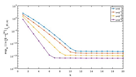
Figure 1: Convergence of 1D case vs. interation number $k$ for different values of $\sigma=0,2^{1},2^{3},2^{5}$.

Subsequently, we choose the damping coefficient $\sigma=2$ to calculate the mean-square error and the convergence order of the proposed parareal algorithm. We compute the numerical solution with the fine step-size $\Delta t=2^{-10}$ and the coarse step-size $\Delta T=2^{-6},2^{-7},2^{-8},2^{-9}$. Tables 1, 2 and 3 report the numerical error and convergence order of the parareal algorithm with the iteration number $k=3,4,5$. It is clearly shown that the mean-square convergence order always increases as the iteration number $k$ increases.

Remark 5.

From a numerical analysis point of view, the inclusion of damping coefficients usually accelerates the convergence of numerical solutions by suppressing oscillations and instability, resulting in a faster steady state or desired precision. However, too small damping may not be enough to accelerate the convergence rate and may even introduce instability.

$\Delta T$	$E_{z}$		$H_{y}$
	$(E\||err||_{L^{2}}^{2})^{1/2}$	order	$(E\||err||_{L^{2}}^{2})^{1/2}$	order
$\frac{1}{2^{6}}$	5.776e-03	–	7.784e-03	–
$\frac{1}{2^{7}}$	3.267e-03	0.822	2.081e-03	1.903
$\frac{1}{2^{8}}$	8.160e-04	2.001	6.337e-04	1.716
$\frac{1}{2^{9}}$	8.744e-05	3.222	9.468e-05	2.743

Table 1: Numerical error and convergence order of 1D case for $k=3$.

$\Delta T$	$E_{z}$		$H_{y}$
	$(E\||err||_{L^{2}}^{2})^{1/2}$	order	$(E\||err||_{L^{2}}^{2})^{1/2}$	order
$\frac{1}{2^{6}}$	4.046e-04	–	2.151e-04	–
$\frac{1}{2^{7}}$	3.995e-05	3.340	3.712e-05	2.535
$\frac{1}{2^{8}}$	5.922e-06	2.754	4.041e-06	3.200
$\frac{1}{2^{9}}$	3.900e-07	3.925	2.475e-07	4.030

Table 2: Numerical error and convergence order of 1D case for $k=4$.

$\Delta T$	$E_{z}$		$H_{y}$
	$(E\||err||_{L^{2}}^{2})^{1/2}$	order	$(E\||err||_{L^{2}}^{2})^{1/2}$	order
$\frac{1}{2^{6}}$	7.704e-06	–	7.808e-06	–
$\frac{1}{2^{7}}$	5.126e-07	3.910	6.239e-07	3.646
$\frac{1}{2^{8}}$	4.229e-08	3.600	3.467e-08	4.170
$\frac{1}{2^{9}}$	5.506e-10	6.263	5.736e-10	5.917

Table 3: Numerical error and convergence order of 1D case for $k=5$.

5.1.2 Two-dimensional transverse magnetic waves

We consider the stochastic Maxwell equations with 2-D transverse magnetic polarization driven by trace class noise

$$\left\{\begin{array}[]{ll}\dfrac{\partial E_{z}}{\partial t}=\dfrac{1}{\varepsilon}(\dfrac{\partial H_{y}}{\partial x}-\dfrac{\partial H_{x}}{\partial y})-\sigma E_{z}+\lambda_{1}\cdot\dot{W},\\[11.38109pt] \dfrac{\partial H_{x}}{\partial t}=-\dfrac{1}{\mu}\dfrac{\partial E_{z}}{\partial y}-\sigma H_{x}+\lambda_{2}\cdot\dot{W},\\[11.38109pt] \dfrac{\partial H_{y}}{\partial t}=\dfrac{1}{\mu}\dfrac{\partial E_{z}}{\partial x}-\sigma H_{y}+\lambda_{2}\cdot\dot{W},\end{array}\right.$$ (46)

by providing initial conditions

$$E_{z}(x,y,0) =\sin(3\pi x)\sin(4\pi y),$$

$$H_{x}(x,y,0) =-0.8\cos(3\pi x)\sin(4\pi y),$$

$$H_{y}(x,y,0) =-0.6\sin(3\pi x)\sin(4\pi y),$$

for $t\in[0,1]$ and $(x,y)\in D=[0,2\pi]\times[0,2\pi]$. Following the formula (6), we choose $e_{n}(x)=\sqrt{2/a}\sin\left(n\pi x/a\right)$ and $\lambda_{n}=n^{-(2r+1+\delta)}$, for some $\delta>0$ and $r\geq 0$. In this case, $Tr\left(Q\right)=\sum_{n=1}^{\infty}\lambda_{n}<\infty$. We construct the Wiener process as follows [8]

$$W(t)=\sqrt{\dfrac{2}{a}}\sum_{n=1}^{\infty}n^{-(\frac{2r+1+\delta}{2})}\sin\left(\frac{n\pi x}{a}\right)\beta_{n}(t),$$

with $a=2,\,r=0.5$ and $\delta=0.001$.

Firstly, the parameters are normalized to $\varepsilon=1$, $\mu=1$ and $\lambda_{1}=\lambda_{2}=1$. We take the fine step-size $\Delta t=2^{-5}$, the coarse step-size $\Delta T=2^{-3}$ and the spatial mesh grid-size $\Delta x=\Delta y=2\pi/50$. Fig. 2 demonstrates the evolution of the mean-square error $(\sup_{1\leq n\leq N}E\|u_{n}^{(k)}-u_{n}^{ref}\|^{2})^{\frac{1}{2}}$ with iteration number $k$. From the Fig. 2, we observe that the error approaches $10^{-13}$ after $k=8$ nearly, which shows that the proposed algorithm converges.

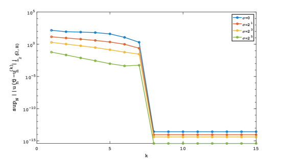
Figure 2: Convergence of 2D case vs. interation number $k$ for different values of $\sigma=0,2^{1},2^{3},2^{5}$.

Secondly, in order to investigate the relationship between the convergence error and the damping coefficient, we consider the numerical error and convergence order of the proposed algorithm as taking the different iteration number $k$ with $\sigma=0$, i.e., transverse magnetic waves in lossless medium will be discussed. We compute the numerical solution with the fine step-size $\Delta t=2^{-7}$ and the coarse step-size $\Delta T=2^{-3},2^{-4},2^{-5},2^{-6}$. Tables 4, 5 and 6 report the numerical error and convergence order of the proposed algorithm with the iteration number $k=3,4,5$. From Tables 4, 5 and 6, we find that the numerical convergence order is affected by the regularity of the noise and the accuracy is not as expected.

Remark 6.

In numerical simulation, the introduction of damping terms and the selection of parameters need to be careful to ensure the accuracy and physical authenticity of simulation results. Excessive damping may lead to excessive attenuation, thus affecting the accuracy of simulation results.

$\Delta T$	$E_{z}$		$H_{x}$		$H_{y}$
	$(E\||err||^{2})^{1/2}$	order	$(E\||err||^{2})^{1/2}$	order	$(E\||err||^{2})^{1/2}$	order
$\frac{1}{2^{3}}$	1.155	–	3.897e-01	–	1.061	–
$\frac{1}{2^{4}}$	3.612e-01	1.676	1.317e-01	1.565	3.683e-01	1.527
$\frac{1}{2^{5}}$	1.398e-01	1.370	5.380e-02	1.291	1.576e-01	1.225
$\frac{1}{2^{6}}$	4.480e-02	1.642	1.210e-02	2.158	4.290e-02	1.878

Table 4: Numerical error and convergence order of 2D case in lossless medium for $k=3$.

$\Delta T$	$E_{z}$		$H_{x}$		$H_{y}$
	$(E\||err||^{2})^{1/2}$	order	$(E\||err||^{2})^{1/2}$	order	$(E\||err||^{2})^{1/2}$	order
$\frac{1}{2^{3}}$	6.122e-02	–	1.197e-02	–	3.187e-02	–
$\frac{1}{2^{4}}$	1.092e-02	2.488	2.245e-03	2.415	5.962e-03	2.4182
$\frac{1}{2^{5}}$	2.548e-03	2.099	2.407e-04	3.221	6.451e-04	3.2081
$\frac{1}{2^{6}}$	2.771e-04	3.200	3.567e-05	2.755	1.165e-04	2.4692

Table 5: Numerical error and convergence order of 2D case in lossless medium for $k=4$.

$\Delta T$	$E_{z}$		$H_{x}$		$H_{y}$
	$(E\||err||^{2})^{1/2}$	order	$(E\||err||^{2})^{1/2}$	order	$(E\||err||^{2})^{1/2}$	order
$\frac{1}{2^{6}}$	1.526e-03	–	3.146e-04	–	1.362e-03	–
$\frac{1}{2^{7}}$	1.090e-04	3.807	3.267e-05	3.268	1.463e-04	3.2187
$\frac{1}{2^{8}}$	1.371e-05	2.992	2.781e-06	3.554	1.313e-05	3.4789
$\frac{1}{2^{9}}$	6.602e-07	4.376	9.392e-08	4.888	5.779e-07	4.5054

Table 6: Numerical error and convergence order of 2D case in lossless medium for $k=5$.

After a proper adjustment, in order to increase the convergence order, we choose the damping coefficient $\sigma=2^{3}$ and $\lambda_{1}=\lambda_{2}=10^{-6}$ to reduce the impact of trace class noise. Similarly, we take the fine step-size $\Delta t=2^{-7}$ and the coarse step-size $\Delta T=2^{-3},2^{-4},2^{-5},2^{-6}$. Tables 7, 8 and 9 report the numerical error and convergence order with the iteration number $k=3,4,5$. Indeed, the numerical experiments reveal that the convergence order of the proposed algorithm increases as the iteration number $k$ increases.

$\Delta T$	$E_{z}$		$H_{x}$		$H_{y}$
	$(E\||err||^{2})^{1/2}$	order	$(E\||err||^{2})^{1/2}$	order	$(E\||err||^{2})^{1/2}$	order
$\frac{1}{2^{3}}$	3.363e-04	–	1.174e-02	–	8.867e-03	–
$\frac{1}{2^{4}}$	1.716e-05	4.292	1.683e-03	2.802	1.231e-03	2.802
$\frac{1}{2^{5}}$	2.462e-06	2.801	5.151e-04	1.709	3.887e-04	1.708
$\frac{1}{2^{6}}$	1.085e-06	1.182	1.502e-04	1.775	1.136e-04	1.778

Table 7: Numerical error and convergence order of 2D case with the damping coefficient $\sigma=2^{3}$ for $k=3$.

$\Delta T$	$E_{z}$		$H_{x}$		$H_{y}$
	$(E\||err||^{2})^{1/2}$	order	$(E\||err||^{2})^{1/2}$	order	$(E\||err||^{2})^{1/2}$	order
$\frac{1}{2^{3}}$	4.665e-04	–	1.256e-02	–	6.529e-02	–
$\frac{1}{2^{4}}$	2.217e-05	4.396	6.140e-04	3.198	7.113e-03	4.355
$\frac{1}{2^{5}}$	3.407e-06	2.702	1.007e-04	2.103	1.656e-03	2.612
$\frac{1}{2^{6}}$	5.420e-07	2.652	1.563e-05	2.459	3.013e-04	2.684

Table 8: Numerical error and convergence order of 2D case with the damping coefficient $\sigma=2^{3}$ for $k=4$.

$\Delta T$	$E_{z}$		$H_{x}$		$H_{y}$
	$(E\||err||^{2})^{1/2}$	order	$(E\||err||^{2})^{1/2}$	order	$(E\||err||^{2})^{1/2}$	order
$\frac{1}{2^{6}}$	2.401e-03	–	8.880e-02	–	6.708e-02	–
$\frac{1}{2^{7}}$	2.991e-04	6.327	3.351e-03	4.728	2.531e-03	4.728
$\frac{1}{2^{8}}$	1.534e-05	4.309	4.039e-04	3.053	3.049e-04	3.053
$\frac{1}{2^{9}}$	3.191e-07	2.058	3.848e-05	3.392	2.905e-05	3.392

Table 9: Numerical error and convergence order of 2D case with the damping coefficient $\sigma=2^{3}$ for $k=5$.

5.2 Impact of the scale of noise

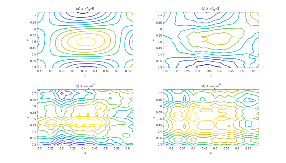
Figure 3: 10 Contour of $E_{z}(x,y)$ with different sizes of noise $\lambda_{1}=\lambda_{2}=0,2^{1},2^{3},2^{5}$ in the time $T=1$.

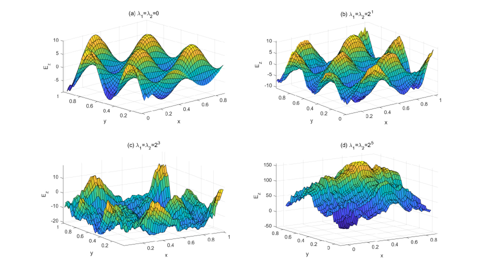
Figure 4: $E_{z}(x,y)$ with different sizes of noise $\lambda_{1}=\lambda_{2}=0,2^{1},2^{3},2^{5}$ in the time $T=1$.

We consider the stochastic Maxwell equations with 2-D transverse magnetic polarization (46). The parameters are normalized to $\varepsilon=1$, $\mu=1$ and we take the fine step-size $\Delta t=2^{-5}$, the coarse step-size $\Delta T=2^{-3}$ and the spatial mesh grid-size $\Delta x=\Delta y=1/50$. In order to show the impact of the scale of noise on the numerical solution, we perform numerical simulations with four scales of noise $\lambda_{1}=\lambda_{2}=0,2^{1},2^{3},2^{5}$ and choose the damping coefficient $\sigma=2^{3}$.

Fig.3 shows the 10 Contour plots of the numerical solution $E_{z}(x,y)$ with different scales of noise and Fig.4 shows the electric field wave forms $E_{z}(x,y)$ with different scales of noise. Comparing with deterministic case (a) of Fig.3 and Fig.4, we can find that the oscillator of the wave forms (b-d) of Fig.3 and Fig.4 becomes more and more violent as the scale of the noise increases, i.e., from (a-d) of Fig.3 and Fig.4 it can be observed that the perturbation of the numerical solutions becomes more and more apparent as the scale of the noise increases.

6 Conclusion

In this paper, we study the strong convergence analysis of the parareal algorithms for stochastic Maxwell equations with damping term driven by additive noise. Firstly the stochastic exponential scheme is chosen as the coarse propagator and the exact solution scheme is chosen as the fine propagator. And we propose our numerical schemes and establish the mean-square convergence estimate. Secondly, both the coarse propagator and the fine propagator choose the stochastic exponential scheme. Meanwhile, the error we considered in this section is the distance between the solution computed by the parareal algorithm and the reference solution generated by the fine propagator. It is shown that the convergence order of the proposed algorithms is linearly related to the iteration number $k$. At last, One- and two-dimensional numerical examples are performed to demonstrate convergence analysis with respect to damping coefficient and noise scale. One key idea from the proofs of two convergence results is that the residual operator in Theorem 2 is related to Lipschitz continuity properties, whereas Theorem 1 concerns the integrability of the exact solution. The future works will include the study for the parareal algorithms for the stochastic Maxwell equations driven by multiplicative noise and other choices of integrators as the coarse and fine propagators.

References

• [1] M. Badieirostami, A. Adibi, H. Zhou, and S. Chow. Wiener chaos expansion and simulation of electromagnetic wave propagation excited by a spatially incoherent source. Multiscale Model. Sim., 8:591–604, 2010.
• [2] G. Bal and Y. Maday. A "parareal" time discretization for non-linear PDE’s with application to the pricing of an American put. Springer, Berlin, 2002.
• [3] C. Bréhier and X. Wang. On parareal algorithms for semilinear parabolic stochastic PDEs. SIAM J. Numer. Anal., 58:254–278, 2020.
• [4] C. Chen. A symplectic discontinuous Galerkin full discretization for stochastic Maxwell equations. SIAM J. Numer. Anal., 59:2197–2217, 2021.
• [5] C. Chen, J. Hong, and L. Ji. Mean-square convergence of a semidiscrete scheme for stochastic Maxwell equations. SIAM J. Numer. Anal., 57:728–750, 2019.
• [6] C. Chen, J. Hong, and L. Ji. Runge-Kutta semidiscretizations for stochastic Maxwell equations with additive noise. SIAM J. Numer. Anal., 57:702–727, 2019.
• [7] C. Chen, J. Hong, and L. Ji. A new efficient operator splitting method for stochastic Maxwell equations. arXiv preprint arXiv:2102.10547, 2021.
• [8] C. Chen, J. Hong, and L. Ji. Numerical approximations of stochastic Maxwell equations: via structure-preserving algorithms. Springer, Heidelberg, 2023.
• [9] C. Chen, J. Hong, L. Ji, and G. Liang. Ergodic numerical approximations for stochastic Maxwell equations. arXiv preprint arXiv:2210.06092, 2022.
• [10] C. Chen, J. Hong, and L. Zhang. Preservation of physical properties of stochastic Maxwell equations with additive noise via stochastic multi-symplectic methods. J. Comput. Phys., 306:500–519, 2016.
• [11] D. Cohen, J. Cui, J. Hong, and L. Sun. Exponential integrators for stochastic Maxwell’s equations driven by itô noise. J. Comput. Phys., 410:109382, 2020.
• [12] X. Dai, L. Bris, F. Legoll, and Y. Maday. Symmetric parareal algorithms for Hamiltonian systems. ESAIM-Math. Model. Numer. Anal., 47:717–742, 2013.
• [13] X. Dai and Y. Maday. Stable parareal in time method for first-and second-order hyperbolic systems. SIAM J. Sci. Comput., 35:A52–A78, 2013.
• [14] M. Gander and E. Hairer. Analysis for parareal algorithms applied to Hamiltonian differential equations. J. Comput. Appl. Math., 259:2–13, 2014.
• [15] M. Gander and S. Vandewalle. Analysis of the parareal time-parallel time-integration method. SIAM J. Sci. Comput., 29:556–578, 2007.
• [16] J. Hong, B. Hou, Q. Li, and L. Sun. Three kinds of novel multi-symplectic methods for stochastic Hamiltonian partial differential equations. J. Comput. Phys., 467:111453, 2022.
• [17] J. Hong, L. Ji, and L. Zhang. A stochastic multi-symplectic scheme for stochastic Maxwell equations with additive noise. J. Comput. Phys., 268:255–268, 2014.
• [18] J. Hong, L. Ji, and L. Zhang. An energy-conserving method for stochastic Maxwell equations with multiplicative noise. J. Comput. Phys., 351:216–229, 2017.
• [19] J. Hong, X. Wang, and L. Zhang. Parareal exponential $\theta$-scheme for longtime simulation of stochastic Schrödinger equations with weak damping. SIAM J. Sci. Comput., 41:B1155–B1177, 2019.
• [20] T. Horsin, I. Stratis, and A. Yannacopoulos. On the approximate controllability of the stochastic Maxwell equations. IMA J. Math. Control. I., 27:103–118, 2010.
• [21] B. Hou. Meshless structure-preserving GRBF collocation methods for stochastic Maxwell equations with multiplicative noise. Appl. Numer. Math., 192:337–355, 2023.
• [22] K. Liaskos, I. Stratis, and A. Yannacopoulos. Stochastic integrodiferential equations in Hilbert spaces with applications in electromagnetics. J. Integral Equations Appl., 22:559–590, 2010.
• [23] J. Lions, Y. Maday, and G. Turinici. A "parareal" in time discretization of PDE’s. C. R. Acad. Sci. Paris Ser. I Math., 332:661–668, 2001.
• [24] G. Roach, I. Stratis, and A. Yannacopoulos. Mathematical analysis of deterministic and stochastic problems in complex media electromagnetics. Princeton University Press, 2012.
• [25] S. Rytov, I. Kravov, and V. Tatarskii. Principles of statistical radiophysics:elements and random fields 3. Springer, Berlin, 1989.
• [26] J. Sun, C. Shu, and Y. Xing. Multi-symplectic discontinuous Galerkin methods for the stochastic Maxwell equations with additive noise. J. Comput. Phys., 461:111199, 2022.
• [27] J. Sun, C. Shu, and Y. Xing. Discontinuous Galerkin methods for stochastic Maxwell equations with multiplicative noise. ESAIM-Math. Model. Num., 57:841–864, 2023.
• [28] S. Wu and T. Zhou. Convergence analysis for three parareal solvers. SIAM J. Sci. Comput., 37:A970–A992, 2015.
• [29] Y. Yan. Galerkin finite element methods for stochastic parabolic partial differential equations. SIAM J. Numer. Anal., 43:1363–1384, 2005.
• [30] K. Zhang. Numerical studies of some stochastic partial differential equations. PhD thesis, The Chinese University of Hong Kong, 2008.
• [31] L. Zhang, C. Chen, and J. Hong. A review on stochastic multi-symplectic methods for stochastic Maxwell equations. Commun. Appl. Math. Comput., 1:467–501, 2019.
• [32] L. Zhang and L. Ji. Stochastic multi-symplectic Runge–Kutta methods for stochastic Hamiltonian PDEs. Appl. Numer. Math., 135:396–406, 2019.
• [33] L. Zhang, W. Zhou, and L. Ji. Parareal algorithms applied to stochastic differential equations with conserved quantities. J. Comput. Math., 37:48–60, 2019.
• [34] Y. Zhou and D. Liang. Modeling and FDTD discretization of stochastic Maxwell’s equations with Drude dispersion. J. Comput. Phys., 509:113033, 2024.