Exciting DeePMD: Learning excited state energies, forces, and non-adiabatic couplings

Abstract

We extend the DeePMD neural network architecture to predict electronic structure properties necessary to perform non-adiabatic dynamics simulations. While learning the excited state energies and forces follows a straightforward extension of the DeePMD approach for ground-state energies and forces, how to learn the map between the non-adiabatic coupling vectors (NACV) and the local chemical environment descriptors of DeePMD is less trivial. Most implementations of machine-learning-based non-adiabatic dynamics inherently approximate the NACVs, with an underlying assumption that the energy-difference-scaled NACVs are conservative fields. We overcome this approximation, implementing the method recently introduced by Richardson [J. Chem. Phys. 158 011102 (2023)], which learns the symmetric dyad of the energy-difference-scaled NACV. The efficiency and accuracy of our neural network architecture is demonstrated through the example of the methaniminium cation CH₂NH${}_{2}^{+}$.

I Introduction

Since its introduction in 2018, the deep potential methodology Zhang et al. (2018a); Zeng et al. (2023) has significantly impacted molecular simulations in physical chemistry, materials physics, and engineering. Even within the past year, we have seen applications in simulation of sodium silicate glassesBertani et al. (2024), solid-state electrolytesBalyakin et al. (2024); Zhang et al. (2024a), study of thermodynamic stability of magnesium alloysHe et al. (2023), modeling infrared spectra of liquid H₂OLi et al. (2024) or ion hydration/exchange at the mineral-water interfaceRaman and Selloni (2024) that would simply not have been computationally feasible otherwise due to the prohibitive cost of ab initio calculations on these high-dimensional and complex systems. While several other machine learning methods for energies and force fields exist, an advantage of the the deep potential methodology is its versatility to simulate a wide range of atomistic systemsZeng et al. (2023).

So far DeePMD has largely, but not exclusively Chen et al. (2018), focussed on systems in their electronic ground-state. Extending it to model the wide range of phenomena arising from electronic excitations and ensuing coupled electron-nuclear dynamics, would mean the simulation of processes such as photosynthesis, vision, optoelectronics, photocatalysis, to name just a few, and light-matter interactions in general, could harness the computational advantage of the DeePMD model. With ab initio methods, the challenge of efficiently modeling excited electronic structure together coupled with the nuclear dynamics tends to limit both the system sizes as well as the time-scales of the simulations, sometimes to the point that the essential points of interest of the phenomena are unattainable. In recent years, different machine-learning methods have enthusiastically stepped in to the non-adiabatic regime to overcome these challenges, at such a pace that already several reviews exist Li and Lopez (2023); Westermayr and Marquetand (2021); Dral and Barbatti (2021); Li et al. (2023). While the earlier developments used kernel ridge regression Hu et al. (2018); Dral, Barbatti, and Thiel (2018), the community moved more towards neural networks (NNs) Chen et al. (2018); Westermayr et al. (2019) to be able to handle large amounts of input data, made available through several softwares Westermayr, Gastegger, and Marquetand (2020); Zhang et al. (2024b); Li et al. (2021).

Most non-adiabatic dynamics simulations use so-called mixed quantum-classical methods, where classical nuclear trajectories are run self-consistently coupling to the electronic system treated quantum-mechanically. Compared with ground-state processes, these simulations require learning of excited state energies, forces, and non-adiabatic coupling vectors (NACVs). The NACV, also known as the derivative coupling, arises from the nuclear kinetic energy operator acting on the molecular wavefunction, and are defined as:

$$\mathbf{d}_{\alpha\beta}(\mathbf{R})=\langle\phi^{\alpha}_{\mathbf{R}}|\nabla_{\mathbf{R}}\phi^{\beta}_{\mathbf{R}}\rangle$$ (1)

where $\mathbf{R}$ are the nuclear coordinates, and $\phi^{\alpha(\beta)}_{\mathbf{R}}$ is the adiabatic (Born-Oppenheimer) electronic wavefunction associated to the energy $E_{\alpha(\beta)}(\mathbf{R})$. Throughout this paper we will use Greek indices $\alpha,\beta$ to refer only to electronic states.

While learning the excited state energies and forces is more or less a straightforward extension of the ground-state case, learning NACVs is particularly challenging because of three reasons. First, they are typically highly localized, becoming singular at conical intersections, ubiquitous in molecules and prime structures at which electronic population transfer occurs Matsika and Krause (2011); Schuurman and Stolow (2018). Machine learning methods tend to struggle with very localized quantities compared with smoother ones. Second, there is an overall sign arbitrariness that requires additional care, and multi-valuedness stemming from the non-analyticity around a conical intersection. Third, while being a vector quantity similar to the force, they are non-conservative unlike the force, which makes the imposition of invariance under molecular symmetry challenging.

The techniques that are currently in use Chen et al. (2018); Westermayr et al. (2019); Westermayr, Gastegger, and Marquetand (2020) to deal with these three issues are inherently approximate. The earlier ones approximate the non-adiabatic coupling from features of the electronic energy surfaces, such as their gaps and gradients Zhu and Nakamura (1997), and are essentially variations of the Landau-Zener approach from the early days of quantum mechanics Lan (1965); Zener and Fowler (1932) that are designed to operate within surface-hopping dynamics; these approaches have the additional advantage of bypassing the computation of the NACVs on the training set in the first place. The existing extension of DeePMD to non-adiabatic dynamics Chen et al. (2018) utilizes such an approximation. A goal would be to learn electronic structure quantities that could be used for general dynamics methods, not just surface-hopping, especially those with a higher accuracy, e.g. Burghardt, Meyer, and Cederbaum (1999); Ben-Nun and MartÃnez (2002); Worth and Burghardt (2003); Saita and Shalashilin (2012); Min, Agostini, and Gross (2015); Martens (2019); Dupuy, Rikus, and Maitra (2024). One approach is to approximate the NACV through the Hessian of the squared energy-gap, as in Ref. Westermayr, Gastegger, and Marquetand (2020), which pointed out the computational advantage of machine-learning second-derivatives compared to the ab initio electronic structure case. However, it is desirable to go beyond this approximation and try to learn the first-principles expression of Eq. (1). To this end, Ref. Westermayr et al. (2019) addresses the first challenge in learning Eq. (1) by using the Hellmann-Feynman theorem to recast the NAC in terms of a numerator over an energy-difference denominator, since the numerator tends to be smoother function, and phase-correction/invariant algorithms are used address the second challenge. However to address the third challenge, an uncontrolled approximation is used in that work in which the numerator is assumed to be a conservative field.

In this work, we overcome the challenges above by implementing a strategy recently proposed by Richardson Richardson (2023) to efficiently and accurately predict the couplings by learning the mapping between their symmetric dyadic and the local chemical environment descriptors of DeePMD. The learned quantity is the bona fide NACV of Eq. (1) with no approximation imposed upon it, so that the machine-learning procedure can make the most of the the data it is trained with.

The manuscript is organized as follows: In Sec. II we describe the computation of the NACVs, describing the conservative field approximation method used in Schnet Westermayr, Gastegger, and Marquetand (2020), the symmetric dyad decomposition of Ref. Richardson (2023), and our method to build the dyad from DeePMD local descriptors. In Sec. III we review elements of theory of neural networks in the context of excited state predictions, focussing on the architecture of DeePMD, and the key modifications we made to incorporate the learning of the NACV. In Sec. IV we give details regarding the training of the NN, and Sec. V shows our results on the photodynamics of the methaniminium cation CH₂NH${}_{2}^{+}$. We present a conclusion in Sec. VI.

II Challenges in learning non-adiabatic coupling vectors

We focus here on attempts to learn the true NACV of Eq. 1 rather than an approximation of it, and we recall the three challenges to compute these that were mentioned in the introduction.

The peaked nature of the NACV can be readily appreciated from a Hellmann-Feynman recasting of Eq. (1), which can be derived by the following argument. Noting that $\nabla_{\bf R}\langle\phi^{\alpha}_{\bf R}|\phi^{\beta}_{\bf R}\rangle=0$ from orthonormality, we deduce ${\bf d}_{\alpha\beta}=-{\bf d}_{\beta\alpha}$, and so, from expanding the left-hand-side of $\nabla_{\bf R}\langle\phi^{\alpha}_{\bf R}|H_{\rm BO}|\phi^{\beta}_{\bf R}\rangle=\delta_{\alpha\beta}\nabla_{\bf R}E_{\alpha}$ we obtain the equality

$$\langle\phi^{\alpha}_{\bf R}|\nabla_{\bf R}H_{\rm BO}|\phi^{\beta}_{\bf R}\rangle=\delta_{\alpha\beta}\nabla_{\bf R}E_{\alpha}({\bf R})+(E_{\beta}-E_{\alpha}){\bf d}_{\alpha\beta}$$ (2)

leading to

$$\mathbf{d}_{\alpha\beta}(\mathbf{R})=\frac{\mathbf{b}_{\alpha\beta}(\mathbf{R})}{E_{\alpha}(\mathbf{R})-E_{\beta}(\mathbf{R})}\;\;\;\text{for}\;\;\alpha\neq\beta$$ (3)

where

$$\mathbf{b}_{\alpha\beta}(\mathbf{R})=\langle\phi^{\alpha}_{\mathbf{R}}|\nabla_{\mathbf{R}}H_{\rm{BO}}|\phi^{\beta}_{\mathbf{R}}\rangle\,.$$ (4)

The highly localized nature of the NACV is manifest in the form of Eq. (3) since energy-levels typically approach each other in localized regions (avoided crossings). More severely, at a CI, the vanishing of the denominator creates a singularity. This motivates to separate the learning of the energies and the learning of the numerator, $\mathbf{b}_{\alpha\beta}(\mathbf{R})$ with the idea that the latter is smooth enough for machine-learning to work well. This deals with the first challenge mentioned in the introduction, but the second and third remain.

Regarding the second challenge, the output from electronic structure codes arbitrarily assign signs to wavefunctions such that the ${\bf b}_{\alpha\beta}({\bf R})$ can randomly switch signs for neighbouring ${\bf R}$, creating havoc in the neural net training which leads to spurious oscillations of the machine-learned NACV. To account for this, a phase-less loss function for NACVs was introduced in the SchNet methodWestermayr et al. (2019); Westermayr, Gastegger, and Marquetand (2020). For each element of the dataset, this has the form:

$$L_{\text{NAC}}=\text{min}\Big{\{}\sum_{\alpha<\beta}^{n}\Big{|}\Big{|}\mathbf{d}^{{\text{Ref}}}_{\alpha\beta}-\mathbf{d}^{\text{ML}}_{\alpha\beta}s_{\alpha}s_{\beta}\Big{|}\Big{|}^{2}\Big{\}},\;s_{\alpha}=\pm 1$$ (5)

where $n$ is the number of electronic states under consideration. Since only the combination of wavefunction signs $\{s_{\alpha}\}$ that minimizes the loss function is used, it ensures the ML prediction will converge to a non-oscillating function as NN functions are inherently smooth. While this phase-less loss function resolves the difficulty of learning quantities of arbitrary signs, it does not however resolve the problem of the multivalued property of the NACVs due to a conical intersection. We will return to this issue shortly.

II.1 Conservative field approximation

Regarding the third challenge, the existing NN codes for non-adiabatic dynamics, SchNet Westermayr, Gastegger, and Marquetand (2020) and PYRAI²MD Li et al. (2021), that go beyond the Landau-Zener type of approximations for the NACV, learn the numerator of NACVs in a similar way to the forces associated to each potential energy surface. That is, they set

$$\mathbf{b}_{\alpha\beta}(\mathbf{R})\approx\nabla_{\mathbf{R}}\big{[}B_{\alpha\beta}\big{]}\,.$$ (6)

Here, $B_{\alpha\beta}$ is a fictitious field which is built from the chemical descriptors in the same way as an energy. It thus gives $\mathbf{b}_{\alpha\beta}(\mathbf{R})$ the same symmetries with respect to the nuclear geometry as a force field, under the approximation that ${\bf b}_{\alpha\beta}({\bf R})$ is a conservative field. To show that in fact $\mathbf{b}_{\alpha\beta}(\mathbf{R})$ is not a conservative field, we consider its curl. When $\alpha\neq\beta$, we have

$$\nabla_{\bf R}\times{\bf b}_{\alpha\beta}({\bf R}) = \nabla_{\bf R}(E_{\beta}({\bf R})-E_{\alpha}({\bf R}))\times{\bf d}_{\alpha\beta}$$ (7)

$$+ (E_{\beta}({\bf R})-E_{\alpha}({\bf R}))(\nabla_{\bf R}\times{\bf d}_{\alpha\beta})$$

There is no reason to expect that either of these terms are zero in general, i.e. even in the absence of a CI, the numerator ${\bf b}_{\alpha\beta}({\bf R})$ is non-conservative and cannot be written as the gradient of a scalar function. In the rest of this paper we will refer to Eq. (6) as the “conservative field approximation” (CFA).

In passing, we note that, although not an NAC, when $\alpha=\beta$ the field ${\bf b}_{\alpha\alpha}({\bf R})$ is conservative in the absence of a conical intersection but non-conservative if there is a conical intersection:

$$\nabla_{\bf R}\times{\bf b}_{\alpha\alpha}({\bf R})=\nabla_{\bf R}\times\nabla_{\bf R}E_{\alpha}({\bf R})$$ (8)

whose curl would be zero in the absence of singularities such as occurs at conical intersections. The non-zero value of the curl yields the Berry phase.

Aside from the unsettling uncontrolled nature of the approximation, a severe consequence of the CFA of Eq. 6 is that NACVs are incorrectly set strictly to zero along any direction perpendicular to a symmetry plane. While the intermolecular force would correctly be zero in that direction, there is no reason for the NACV to be. We will illustrate an example of this in Sec. V. This would lead to a significant underestimation of electron population transfer in these situations, since the out-of-plane motion funneling the transfer is missed.

II.2 Symmetric dyad matrix

We will implement the approach of Richardson which, while motivated in the original work Richardson (2023) by confronting the multivalued character of the NACV, in fact also overcomes all the challenges above. The central object is an auxiliary quantity, the symmetric dyad of $\mathbf{b}_{\alpha\beta}(\mathbf{R})$, and it allows us to learn NACVs more rigorously keeping with its original definition Richardson (2023).

The symmetric dyad of $\mathbf{b}_{\alpha\beta}(\mathbf{R})$ is defined as Richardson (2023):

$$\Gamma_{\alpha\beta}(\mathbf{R})=\mathbf{b}_{\alpha\beta}(\mathbf{R})\;\big{(}\mathbf{b}_{\alpha\beta}(\mathbf{R})\big{)}^{T}$$ (9)

As a real symmetric matrix $\Gamma_{\alpha\beta}\in\mathbb{R}^{3N\times 3N}$, it has one non-zero eigenvalue $\lambda=||\mathbf{b}_{\alpha\beta}(\mathbf{R})||^{2}$ associated to the eigenvector $\mathbf{b}_{\alpha\beta}(\mathbf{R})/\sqrt{\lambda}$. This makes recovering the NACVs from their symmetric dyad straightforward.

By learning $\Gamma_{\alpha\beta}$, there is no inherent approximation as there is with the CFA. Two further advantages of this auxiliary field are its single-valuedness and its independence to phase factors in electronic wavefunction. During a dynamical simulation, phase tracking along trajectory allows to retrieve the phase accumulated when encircling a conical intersection, thus recovering Berry phase effects lost in the CFA. We return to the specific details of how we learn $\Gamma_{\alpha\beta}$ in Sec. III.3.

III DeePMD Neural Network architecture

Over the years the DeePMD community has developed a great variety of schemes to encode chemical information Wang et al. (2022); Zeng et al. (2023). Here, we focus our discussion only on approaches that either are used in the present work or are relevant to predict vector properties. We encourage the reader to consult Ref. Zeng et al. (2023) for an overview. We start this section with the building blocks of DeePMD’s efficient prediction of electronic structure properties from the local chemical environment.

We distinguish the vector $\mathbf{R}$ containing all nuclear coordinates from $\mathbf{r}_{i}=(x_{i},y_{i},z_{i})$ containing only the cartesian coordinates of atom $i$.

III.1 Embedding

DeePMD relies on the fundamental idea that electronic properties should be obtainable as a sum of atom-wise contributions that only depend on atomic interactions between neighbors, up to a certain distance. To each atom $i$ is associated its own descriptor encoding only the position of neighboring atoms up to a cut-off radius $r_{c}$ (see below). All descriptors considered in this work are built upon a smoothly-decaying coordinate matrix of neighboring atoms with rows Zhang et al. (2018b):

$$\left(\mathcal{R}^{i}\right)_{j}=\left\{s(r_{ij})\quad\frac{s(r_{ij})x_{ij}}{r_{ij}}\quad\frac{s(r_{ij})y_{ij}}{r_{ij}}\quad\frac{s(r_{ij})z_{ij}}{r_{ij}}\right\}$$ (10)

where $\mathbf{r}_{ij}=\mathbf{r}_{j}-\mathbf{r}_{i}=(x_{ij},y_{ij},z_{ij})$ and $r_{ij}=||\mathbf{r}_{ij}||$. Thus $\mathcal{R}^{i}\in\mathbb{R}^{N_{c}\times 4}$ where $N_{c}$ is the expected maximum number of neighbors within the cut-off radius $r_{c}$. The role of the switching function $s(r)$ is to control the ability of neighboring atoms to influence each other by smoothly transitioning from an inverse distance function to a fast-decaying polynomial depending on cut-off hyper-parameters tweaked by the user:

$$s(r)=\left\{\begin{tabular}[]{l l}$\displaystyle\frac{1}{r}$&\; $r<r_{s}$,\\ \\ $\displaystyle\frac{1}{r}\left[q^{3}(-6q^{2}+15q-10)+1\right]$&\; $r_{s}\leq r<r_{c}$,\\ \\ $0$&\; $r\geq r_{c}$\end{tabular}\right.$$ (11)

where $\displaystyle q=\frac{r-r_{s}}{r_{c}-r_{s}}$ and $r_{s}$ is a parameter controlling the smooth turn-off within the local region. The design of the switching function is explained in Refs. Zhang et al. (2018b); Zeng et al. (2023). As it is continuous up to the second-order derivative, $s(r)$ is sufficiently smooth to be used in descriptors that in turn will feed fitting networks predicting energies and forces.

The generalized coordinate matrices $\mathcal{R}^{i}$ are invariant with respect to system translation, but lack the invariance with respect to rotation. Thus, they are not bona fide descriptors, but will constitute their building blocks. One of the strengths of DeePMD is to include a machine learning component in the design of descriptors in complement to the fitting networks they will be fed into. Different descriptor types are distinguished by how much information is fed to this embedding neural network.

The so-called 2-body embedding descriptor only feeds radial information to the embedding NN, denoted $\mathcal{N}_{e,2}$:

$$\left(\mathcal{G}^{i}\right)_{j}=\mathcal{N}^{p_{ij}}_{e,2}\big{(}s(r_{ij})\big{)}$$ (12)

where it is understood that each line of $\mathcal{G}^{i}\in\mathbb{R}^{N_{c}\times M}$ is obtained by feeding one scalar value $s(r_{ij})$ to the embedding NN $\mathcal{N}_{e,2}$, returning values of its final neuron layer of width $M$. A specific set of parameters (weights and biases) for $\mathcal{N}_{e,2}$ is used depending on the atomic species of the atom pair ${p_{ij}}$. This ensures that the descriptor satisfies permutation symmetry, and reduces complexity. The full embedding descriptor of atom $i$ is built following:

$$\mathcal{D}^{i}=\frac{1}{N_{c}^{2}}\left(\mathcal{G}^{i}\right)^{T}\theta^{i}\;\mathcal{G}^{i}_{<}$$ (13)

where $\theta^{i}=\left(\mathcal{R}^{i}\right)\left(\mathcal{R}^{i}\right)^{T}$ encodes the angular information (’angle form’ of Ref. Zeng et al. (2023) ) of two neighbors $j$ and $k$ and with $\mathcal{G}^{i}_{<}\in\mathbb{R}^{N_{c}\times M_{<}}$ taking only the first $M_{<}$ columns of $\mathcal{G}^{i}$ to reduce the size of $\mathcal{D}^{i}\in\mathbb{R}^{M\times M_{<}}$. We emphasize that formally, the features of this descriptor encode information beyond 2-body terms. The name only refers to the amount of information that is fed to the embedding NN. By design, this descriptor is invariant under permutation symmetry and overall translations/rotations of the system.

Better accuracy can be achieved when 3-body terms are fed to the embedding NN Wang et al. (2022), denoted $\mathcal{N}_{e,3}$. In this case, tensor $\mathcal{G}^{i}\in\mathbb{R}^{N_{c}\times N_{c}\times M}$ contains embedding NN features obtained as :

$$\left(\mathcal{G}^{i}\right)_{jk}=\mathcal{N}_{e,3}^{p_{jk}}\left((\theta^{i})_{jk}\right)$$ (14)

where it is understood that the neural network is separately fed with each scalar $(\theta^{i})_{jk}$ and outputs a vector of $M$ features where $M$ is the width of the final neuron layer. A specific set of NN parameters is used for every pair of atomic species $p_{jk}$, similar to what is done for 2-body embedding. The full embedding descriptor of atom $i$ reads:

$$\mathcal{D}^{i}=\frac{1}{N_{c}^{2}}\,\theta^{i}:\mathcal{G}^{i}$$ (15)

The notation ”$:$” represents the contraction between matrix $\mathcal{R}^{i}\left(\mathcal{R}^{i}\right)^{T}$ and the first two dimensions of tensor $\mathcal{G}^{i}$. As desired, this descriptor is invariant under permutation symmetry and overall rotation/translation of all atoms.

We now recall how energies and forces are predicted from those descriptors.

III.2 Property prediction: energies and forces

A separate energy predictor will be associated to each electronic state $\alpha$. We describe its structure for one state only without loss of generality. Following the principle of atomic embedding, each atomic descriptor $\mathcal{D}^{i}$ is fed to a fitting network $\mathcal{F}_{\alpha}$ outputing a single scalar (zero-order tensor) interpreted as an atom-wise energy contribution. The total energy is recovered as the sum over atoms:

$$E_{\alpha}=\sum_{i=1}^{N}E_{\alpha,i}=\sum_{i=1}^{N}\mathcal{F}_{\alpha}^{a_{i}}(\mathcal{D}^{i})$$ (16)

where the $a_{i}$ superscript in $\mathcal{F}^{a_{i}}_{0}$ indicates that atoms of the same species $a_{i}$ share the same parameters in the fitting network. In turn, the force is recovered through automatic differentiation of the NN prediction of $E_{\alpha}$ with respect to atomic positions:

$$\mathbf{F}_{\alpha}=-\nabla_{\mathbf{R}}E_{\alpha}$$ (17)

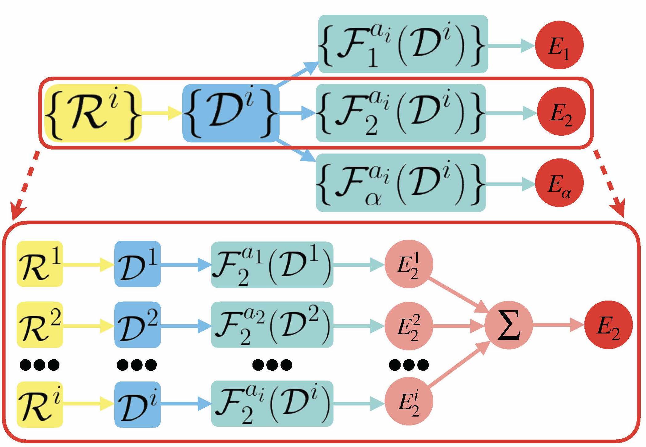
Figure 1: NN architecture for energy prediction. Coordinate matrices (yellow) are built for each atom local environment. They are then used to assemble descriptors (blue) with a 2-body embedding NN component. This collection of descriptor features is shared between all prediction components (green), each outputing the energy of a different state (red). A detailed view of the atom-wise contributions is shown for the first excited state. The NN architecture for NACV prediction within the CFA is similar in structure.

To compute the energies and forces of $n$ electronic states, extending the framework of DeePMD is straightforward: One can simply build a separate instance of the usual DeePMD architecture for each state considered, with descriptor and predictor components.

However, in order to reduce computational complexity, we will use only one instance of the 2-body embedding descriptors of Eq. (13). This descriptor will be fed to all $n$ energy/force prediction components. Figure 1 schematizes the architecture used for energy prediction. Parts of the NN dedicated to prediction of energy/forces are made completely independent from the components dedicated to predicting the NACVs (more precisely, $\mathbf{b}_{\alpha\beta}$). This is not a strict rule. It allows us to focus our attention on the learning of couplings, as learning the energy surfaces and forces is more routine. However, within both parts of the architecture, prediction of the different states/coupling will not be independent from the others as they will share embedding descriptors. In addition to a decrease in complexity, an advantage of sharing descriptors between many prediction components is that it forces the embedding NNs to learn more general properties about the system than if one different embedding descriptor was generated per electronic state. Because it is put under greater constraint, the NN will be less prone to overfitting as a result.

For completeness, we mention a method for the prediction of vector properties which cannot be obtained as the gradient of a field, developed in DeepMD communityZeng et al. (2023) for the prediction of polarization Zhang et al. (2020) through maximally localized Wannier functions. After a fitting network $\mathcal{F}_{1}$ is fed with local atomic descriptor $\mathcal{D}^{i}$ given by Eq. (13), it outputs its last neuron layer of width $M$ which is combined with the coordinate matrix and embedding NN of Eq. (12) in the following way:

$$\begin{split}\left(V_{i}\right)_{x}&=\frac{1}{N_{c}}\sum_{j=1}^{N_{c}}\sum_{m=1}^{M}\left(\mathcal{G}^{i}\right)_{jm}\left(\mathcal{R}^{i}\right)_{j,x+1}\left(\mathcal{F}_{1}(\mathcal{D}^{i})\right)_{m}\,\\ &x=1,2,3\end{split}$$ (18)

A 3-dimensional full vector may be recovered by summing atom-wise contributions: $\displaystyle\mathbf{V}=\sum_{i}^{N}\mathbf{V}_{i}$.

Of present interest, we might consider whether this approach could be used to learn our NACV, however upon inspection, one realizes it would suffer from the problem described in the last paragraph of Sec. II.1: Notice it effectively takes the vector space of all $\left(\mathcal{R}^{i}\right)_{j}$ as a basis to build vectors. When the molecule approaches a planar geometry, this basis lacks any vector perpendicular to that plane, and thus cannot represent non-adiabatic couplings faithfully.

III.3 Predicting NACVs via their symmetric dyad

We now turn to our main contribution in this paper: to extend DeePMD to predict NACVs through learning the symmetric dyad matrix Eq. (9) described in Sec. II.2. While Ref. Richardson (2023) proposed the general approach, so far there has been no NN scheme to actually predict $\mathbf{\Gamma}$. Since the size of the matrix scales quadratically with the number of atoms and its elements can depend on up to two atom displacements, the question of how to build it efficiently from local descriptors is indeed nontrivial. Our method is detailed below.

As we do not have a conservative field, we cannot rely on automatic differentiation to get vector components from a scalar field. Moreover, we cannot learn an effective vector from which to build $\Gamma$ as the multi-valuedness problem would reemerge. We thus need to predict elements of $\Gamma$ separately. The approach usually relied upon in DeePMD to build tensorial properties, such as the polarizability tensorSommers et al. (2020), cannot be used for the reason mentioned at the end of Sec. III.2 concerning vector prediction. Hence, we devised a new approach exploiting symmetries of $\Gamma$ and the atomic embedding principle of DeePMD.

We learn $\Gamma_{\alpha\beta}$ for each pair of states $\alpha,\beta$ as a collection of 3 by 3 blocks

$$\Gamma_{\alpha\beta}=\begin{bmatrix}\Gamma^{11}&\Gamma^{12}&\Gamma^{13}&.\\ \Gamma^{21}&\Gamma^{22}&\Gamma^{23}&.\\ .&.&.&.\end{bmatrix}_{\alpha\beta}$$ (19)

where each block has the structure

$$\Gamma_{\alpha\beta}^{ij}=\begin{bmatrix}\Gamma^{ij}_{xx}&\Gamma^{ij}_{xy}&\Gamma^{ij}_{xz}\\ \Gamma^{ij}_{yx}&\Gamma^{ij}_{yy}&\Gamma^{ij}_{yz}\\ \Gamma^{ij}_{zx}&\Gamma^{ij}_{zy}&\Gamma^{ij}_{zz}\end{bmatrix}_{\alpha\beta}$$ (20)

Blocks on the diagonal $i=j$ are obtained from components of the NACV associated to a single atom, and thus the descriptor $\mathcal{D}^{i}$ associated to it will suffice. It is fed to a fitting neural network set to output the diagonal block. More precisely, only the upper triangular block needs to be predicted, the lower part will be obtained by symmetry:

$$\Gamma_{\alpha\beta}^{ii}=\mathcal{F}_{\alpha\beta}^{ii}\left(\mathcal{D}^{i}\right)\,.$$ (21)

The off-diagonal blocks contain information related to two atoms, so the descriptors $\mathcal{D}^{i}$ and $\mathcal{D}^{j}$ associated to both relevant atoms should be fed to the fitting neural networks. We take the simple strategy to hybridize the two descriptors and feed them to the prediction NN. All elements of off-diagonal blocks are different in principle, and they will be obtained explicitly from the fitting network:

$$\Gamma_{\alpha\beta}^{ij}=\mathcal{F}_{\alpha\beta}^{ij}\left((\mathcal{D}^{i},\mathcal{D}^{j})\right)$$ (22)

To reduce the complexity and enforce permutation symmetry, NN parameters of diagonal blocks $\mathcal{F}_{\alpha\beta}^{ii}$ will be shared for all atoms of same species, and similarly for all pair of species in off-diagonal block predictors $\mathcal{F}_{\alpha\beta}^{ij}$.

We then have to account for the effect of overall rotation of the system on blocks of $\mathbf{\Gamma}$. To this end, we use rotation matrices $\Omega^{i}$ linked to local frames of each atom. The specific choice of definition for the local frames does not matter as long as it evolves continuously with deformation of the molecule. For our test example of CH₂NH${}_{2}^{+}$, we simply define the $z$-axis along the CN bond for all $\Omega^{i}$, while the $x$-axis depends on atom $i$. If it is a hydrogen, the $xz$-plane contains the H atom and the CN bond. Orthogonality allows to deduce where the $x$ and $y$ axes lie. For C and N atoms, a hydrogen atom was picked to define the $xz$ plane as explained above.

Each predicted block of $\Gamma_{\alpha\beta}$ obtained from Eqs. (21) and (22) is then rotated according to

$$\Gamma_{\alpha\beta}^{ij}\longrightarrow\Omega^{i}\;\Gamma_{\alpha\beta}^{ij}\;(\Omega^{j})^{T}$$ (23)

The last step in building our NN architecture is to provide the descriptors $\mathcal{D}^{i}$. Numerical tests show existing DeePMD descriptors lead to important errors on $\Gamma_{\alpha\beta}^{ij}$. Two-body embedding incorrectly predicts same values of NACV components for geometries differing by a rigid torsional motion around the C-N bond. It is important to underline that this shortcoming is the consequence of the different way we use atom-wise descriptors to predict couplings: We do not sum atom-wise contributions as when predicting energies, instead each atom-wise descriptor should hold sufficient information to predict a (diagonal) block of $\Gamma_{\alpha\beta}$. The three-body embedding descriptor does hold more angular information and using Eq. (15) did result in a clear improvement, but not to a completely satisfactory level. We observe that the angular information is essentially ’summed over’, which was not a problem in the context of force prediction through automatic differentiation since the gradient of this descriptor would contain this information, but our approach avoids this since our field is not conservative.

To remedy this, we introduce a new descriptor built on the same elements as the 3-body descriptor described above. We first feed the angle information to an embedding neural network to obtain $\mathcal{G}^{i}=\mathcal{N}_{e,3}\left(\theta^{i}\right)\in\mathbb{R}^{N_{c}\times N_{c}\times M}$. Then, to each matrix $N_{c}\times N_{c}$ matrix contained in $\mathcal{G}^{i}$, we apply successive matrix multiplications with the last three columns of $\mathcal{R}^{i}$ from the right and its transpose from the left. This defines the intermediate descriptor $\mathcal{D}^{i}\in\mathbb{R}^{M\times 3\times 3}$:

$$\left(D^{i}\right)_{m}=\sum_{k=1}^{N_{c}}\sum_{l=1}^{N_{c}}\Big{(}\left(\tilde{\mathcal{R}}^{i}\right)_{k}\Big{)}^{T}\left(\mathcal{G}^{i}\right)_{klm}\;\left(\tilde{\mathcal{R}}^{i}\right)_{l}$$ (24)

$$\left(\tilde{\mathcal{R}}^{i}\right)_{k}=\left\{\frac{s(r_{ik})x_{ik}}{r_{ik}}\quad\frac{s(r_{ik})y_{ik}}{r_{ik}}\quad\frac{s(r_{ik})z_{ik}}{r_{ik}}\right\}$$ (25)

Notice that, unlike the three-body descriptor of Eq. (15), this descriptor does not contract angular information. The fact that angular information is not summed over would ease the job of the prediction layer, but it also means the descriptor is not rotationally invariant. We need to enforce invariance before feeding it to a fitting network. To this end, we again make use of rotations matrices introduced above:

$$\mathcal{D}^{i}=\sum_{k=1}^{N_{c}}\sum_{l=1}^{N_{c}}\Big{(}\left((\Omega^{i})^{T}\tilde{\mathcal{R}}^{i}\right)_{k}\Big{)}^{T}\left(\mathcal{G}^{i}\right)_{klm}\;\left((\Omega^{i})^{T}\tilde{\mathcal{R}}^{i}\right)_{l}$$ (26)

Our method overcomes all above-mentioned limitations of the CFA and previous DeePMD strategies while being numerically efficient by sticking to the atomic embedding principle.

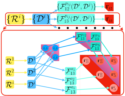
Figure 2: NN architecture for dyad prediction. Coordinate matrices (yellow) are used to construct our generalized descriptors (blue) with a 3-body embedding NN component. This collection of descriptor features is shared between all prediction components (cyan) outputing the (upper triangular parts of) dyads of all required couplings. Atom-wise contributions within the components are shown for the coupling between states 1 and 3. Detail of the prediction of diagonal and off-diagonal blocks of the dyad is sketched.

In our application of the dyad matrix method, the architecture thus separates prediction of energies/forces from prediction of (the numerator of the) NACVs.

To predict the couplings between the $n$ states, $n(n-1)/2$ different $\mathbf{\Gamma}_{\alpha\beta}$ matrices need to be built. To do so, a specific prediction component per coupling will be built, with 3-by-3 sub-blocks of $\mathbf{\Gamma}$ predicted using fitting NNs defined in Eq. (22). Following the same principle as before, all those prediction components will be fed with the same single instance of descriptor given by Eq. (24). Figure 2 sketches the architecture for dyad prediction.

For clarity and conciseness, we presented the architectures omiting the fact that NN parameters are shared between atoms of same species $a_{i}$ or pair of species $p_{ij}$. If we view two NNs of the same structure but with different weights and biases as two separate entities, we remind the reader that there will be as many $\mathcal{N}_{e,3}^{p_{jk}}$ as there are different pairs of atomic species, and similarly for $\mathcal{F}_{\alpha\beta}^{jk}$. Skip connectionHe et al. (2016) with randomized weights lying within the range $0.1\,\pm\,0.001$ was used in all NNs.

IV Training method

We now turn to the methods used for training the NNs. We developed an in-house python code using JAXBradbury et al. (2018), FLAXHeek et al. (2023), and OPTAXDeepMind et al. (2020) to define the NNs and setup the training.

IV.1 Loss functions

We train the NN using Adam stochastic gradient descent methodKingma and Ba (2014) combined with weight decay Loshchilov and Hutter (2017).

The loss function comprises L2 losses associated to the energies, forces and NACVs:

$$L_{\text{D}}=L_{E}+L_{\mathbf{F}}+L_{\mathbf{\Gamma}}\,.$$ (27)

For the energies we have

$$L_{E}=\frac{1}{N_{b}}\displaystyle\sum_{l}^{N_{b}}\sum_{\alpha}^{n}\Big{|}E_{l,\alpha}^{\text{Ref}}-E_{l,\alpha}^{\text{ML}}\Big{|}^{2}$$ (28)

where $N_{b}$ is the total number of elements in the training batch. Similarly, for the forces we define

$$L_{\mathbf{F}}=\frac{1}{N_{b}}\displaystyle\sum_{l}^{N_{b}}\sum_{\alpha}^{n}\Big{|}\Big{|}\mathbf{F}_{l,\alpha}^{\text{Ref}}-\mathbf{F}_{l,\alpha}^{\text{ML}}\Big{|}\Big{|}^{2}\,,$$ (29)

where $||\mathbf{v}||^{2}$ denotes the averaged square of all components of the vector $\mathbf{v}$, and for the symmetric dyad,

$$L_{\mathbf{\Gamma}}=\frac{1}{N_{b}}\displaystyle\sum_{l}^{N_{b}}\sum_{\alpha<\beta}^{n}\Big{|}\Big{|}\mathbf{\Gamma}_{l,\alpha\beta}^{\text{Ref}}-\mathbf{\Gamma}_{l,\alpha\beta}^{\text{ML}}\Big{|}\Big{|}^{2}\,.$$ (30)

IV.2 Input and output normalization

Input and output normalization are used to facilitate the search for the optimal learning rate and control the range spanned by features throughout the neuron layers. Letting $x$ represent the coordinates or energies in the training set of size $N_{s}$, we use its mean $\bar{x}$ and standard deviation $\sigma_{x}$,

$$\bar{x}=\frac{1}{N_{s}}\sum_{l}^{N_{s}}x_{l}\;\;\;{\rm and}\;\;\;\sigma_{x}=\sqrt{\frac{1}{N_{s}}\sum_{l}^{N_{s}}\Big{(}x_{l}-\bar{x}\Big{)}^{2}}\,.$$ (31)

to normalise the values of the switching function $s(x)$ in the following way:

$$\tilde{x}_{l}=\frac{x_{l}-\bar{x}}{\sigma_{x}}$$ (32)

The normalized coordinates are fed into the NN while the normalized reference energies are fed into the loss function. This implies that the forces are to be normalized as well following

$$\tilde{\mathbf{F}}_{\alpha,l}=\frac{\mathbf{F}_{\alpha,l}}{\sigma_{E_{\alpha}}}.$$ (33)

Energies and forces corresponding to a given electronic state $\alpha$ are normalized independently from other states.

Concerning the NACvs, $\mathbf{\Gamma}$ matrices in the loss function are normalized following:

$$\tilde{\mathbf{\Gamma}}_{\alpha\beta,l}=\frac{\mathbf{\Gamma}_{\alpha\beta,l}}{\displaystyle\sqrt{\frac{1}{N_{s}}\sum_{l}^{N_{s}}\mathbf{\Gamma}_{\alpha\beta,l}^{2}}}$$ (34)

Each coupling between a pair of states is normalized separately over the dataset. After training, then the NN will be used to run dynamics, its outputs will be rescaled inversely.

IV.3 Hyperparameter optimization

Hyperparameter optimization will rely on a training dataset and a smaller validation dataset that will be described in next section. We start the optimization of hyperparameters with the determination of an optimal learning rate. During this phase, only the performance on the training set is monitored. To do so, a relatively small ML structure is used to speed-up the numerous training processes that are performed at this stage. To learn energies and forces, embedding/fitting NNs are built with 3 neuron layers of width $M=32$ and a value $M_{<}=12$ for the 2-body embedding descriptor (see Eq. (13)). To learn $\mathbf{\Gamma}$ matrices, separate 3-body descriptors are built from their own embedding NN composed of 3 neuron layers of width $M=32$. They are then fed to fitting networks with 3 neuron layers of width $M=32$.

Initially, the learning rate is sampled uniformly (in logscale) in the range $[0.01,0.00001]$ and training is stopped early, at 625 epochs. The batch size was set to 50. After 3 cycles of refining the grid for the sampling of the rate in the range of optimal performances, the best performing learning rate $\gamma^{(0)}_{\rm best}=0.0012$ is kept. We follow-up by increasing the number of training epochs to $2500$, set the initial learning rate to $\gamma^{(0)}_{\rm best}$ and sample different values of final learning rate uniformly in the range $[0.0012,0.00001]$. The transition from initial to final learning rate is done by exponential decay, the learning rate being changed every 10 descent steps. The optimized value was $\gamma^{(f)}_{\rm best}=0.00005$. We keep the best performing values of initial/final learning rate going forward.

We then increase the width $M$ of each neuron layer until a balance is struck between maximizing accuracy and preventing overfitting. This is done by checking the ability of the NN to learn the training dataset while performing well on the validation set. In the present study, we consider the reproduction of population dynamics obtained without ML as the true ’test’ of our NN (see Results), as the Ab Initio trajectories used as reference are not part of the datasets used. A value of $M=40$ for all NN widths together with a weight decay coefficient of $0.005$ allowed a satisfying performance. We kept $M_{<}=12$ to minimize computational cost.

Owing to the molecular scale of the systems considered in the present work, optimization of the number of atoms included in the local environment descriptors is superfluous at the start of the hyperparameter search. We thus started with cutoff radii of $r_{s}=11.8$ a.u. and $r_{c}=12$ a.u. so that all atoms are included in their respective neighborhood in previous trainings. Then, cutoff were decreased to the minimum values which did not compromise accuracy. Those values turned out to be $r_{s}=5$ a.u. and $r_{c}=7$ a.u.

V Results: the methaniminium cation CH₂NH${}_{2}^{+}$

We use the methaniminium cation to test our implementation, paying particular attention to the prediction of the NACVs. This system was used in the work of Ref. Westermayr et al. (2019); Westermayr, Gastegger, and Marquetand (2020) to test their implementation of machine-learned energies, forces, and NACVs in the Schnet code. We use the data provided in this previous study Westermayr et al. (2019), comprised of a training set of 4000 datapoints and a validation set of 774 datapoints, obtained using the MR-CISD(6,4)/aug-cc-pVDZ electronic structure method. Those data were phase-corrected by the original authors, but we note that our dyad method is impervious to any phase choices.

V.1 Performances on the dataset

We first compare the capability of the CFA and the dyad method to learn the NACV orientation. We refer to the molecular plane at equilibrium geometry as the $xy$-plane in the following. In Figure 3, machine-learned values of $y$ components of $b_{\alpha\beta}$ are plotted against reference values over the whole dataset. Panel (a) and (b) are obtained using CFA and dyad method, respectively. The CFA is seen to prevent the NN to learn the out-of-plane component, even to a qualitative level. In addition to the numerous values predicted as essentially zero for near-to-planar geometries, the whole set is learned with a much lesser accuracy compared to the dyad method, as illustrated in Table 1 where the mean absolute error (MAE) and root mean square error (RMSE) are given for each method, separating each cartesian component of $b_{\alpha\beta}$. This shows that the underlying assumption in CFA of zero curl of ${\bf b}_{\alpha\beta}$ has a significant error in its accuracy. The dyad method has no such inherent approximation and the machine-learned values are significantly more accurate, particularly along the molecular plane of symmetry.

Table 1: Mean absolute error (MAE) and root mean square error (RMSE) on $b_{\alpha\beta}$ over the training set using dyad method and CFA for each cartesian component.

Method	MAE (RMSE) [ $10^{-3}$ a.u.]
	$x$	$y$	$z$
CF	5.4 (8.2)	16 (24)	8.0 (14)
Dyad	2.0 (3.5)	2.3 (3.8)	2.2 (4.4)

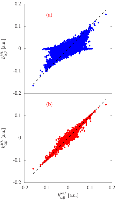
Figure 3: Performance of ML methods to reproduce out-of-plane $b_{\alpha\beta}$ components on the training set. Learned values are plotted against reference values. Panel (a): CFA. Panel (b): dyad method.

V.2 SHEDC dynamics

We performed surface-hopping with energy-based decoherence correction (SHEDC) dynamics Granucci and Persico (2007); Granucci, Persico, and Zoccante (2010) using our NN with dyad method to supply energies, forces and NACVs. Details regarding initial conditions and dynamical parameters are identical to that of Ref Westermayr et al. (2019), and recalled below. We used a total of 1000 trajectories, for which initial conditions were obtained via Wigner sampling along normal modes taken at the ground state equilibrium geometry. We checked that at all initial conditions, the machine-learned energy gap between $S_{0}$ and $S_{2}$ lay within $9.44\pm 0.15$ eV. They were then propagated for 100 fs, starting in $S_{2}$. The integration timestep was set to 0.5 fs for nuclear motion, with 25 electronic timesteps performed within each nuclear timestep. As NACVs are defined up to an arbitrary sign, phase tracking was performed along the trajectories. Velocity rescaling is performed along NACVs, and frustrated hops result in reversing the velocity.

In Figure 4 we compare the resulting population dynamics (dashed orange lines) to reference results of 90 trajectories propagated from the MR-CISD(6,4)/aug-cc-pVDZ electronic structure method (solid black lines). The agreement is very satisfactory, and is compared to previous results of Ref Westermayr, Gastegger, and Marquetand (2020) using ML relying on the CFA to replace the ab initio calculations. All ML results shown in Figure 4 exploit NNs that were trained on the same dataset, comprised of 4000 datapoints that were phase-corrected before trainingWestermayr et al. (2019). All population dynamics obtained through ML employ the same number of trajectories. Panel (a) shows results using CFA together with the phase-less loss Eq. (5) during training of the NN in blue dashed lines. The green-dashed lines in panel (b) also shows the CFA but using instead the L2 loss, $L_{\text{NAC}}=\frac{1}{N_{b}}\displaystyle\sum_{l}^{N_{b}}\sum_{\alpha<\beta}^{n}\Big{|}\Big{|}\mathbf{d}_{l,\alpha\beta}^{\text{Ref}}-\mathbf{d}_{l,\alpha\beta}^{\text{ML}}\Big{|}\Big{|}^{2}$ during training. As the dataset is pre-processed through a phase correction scheme, use of the phase-less loss function rather than L2 loss should yield the same accuracy if this pre-processing is robust. However, the NN trained using the L2 loss is seen to predict slightly slower population transfer from $S_{2}$ to $S_{1}$ during the first 20 fs and from $S_{1}$ to $S_{0}$ at later times. We attribute these variations to the non-rigorous character of the dataset phase pre-processing, aiming at making a single-valued, smooth NACV field out of a fundamentaly multi-valued oneRichardson (2023). Moreover, both CFA-based results exhibit slower population transfer from $S_{2}$ to $S_{1}$ at early times compared to Ab Initio results. Our dyad method yields population dynamics in excellent agreement with Ab Initio during the first 50 fs, followed by a slightly slower population transfer between $S_{1}$ and $S_{0}$ at later times. Owing to the limited size of the training dataset, together with the fact it was generated from adaptive sampling relying on the CFA approximationWestermayr et al. (2019), it is possible our dyad trajectories explore a region of configuration space that was not sampled as comprehensively. Moreover, as only 90 Ab Initio trajectories were propagated, it is not certain the Ab Initio populations dynamics do not suffer from undersampling at later times. We are thus led to consider our quantitative prediction for early times as a significant proof of the robustness of our dyad method.

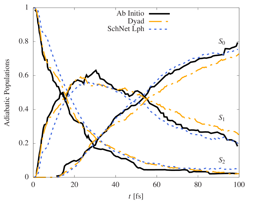
(a)

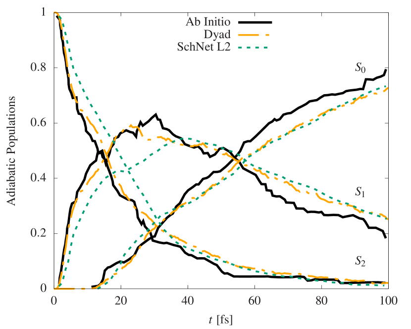
(b)

Figure 4: Comparison of population dynamics relying on explicit MR-CISD(6,4) calculations (Ab Initio, see Ref Westermayr et al. (2019)) in black solid lines to our results using the dyad method in orange dashed lines. On panel (a), results of Ref Westermayr, Gastegger, and Marquetand (2020) using the CFA and phaseless loss in training is shown in blue dashed lines. On panel (b), results using L2 loss are shown in green dashed lines. All NNs were trained on a phase-corrected dataset.

Lastly, we compare our results using the dyad method (orange dashed lines) to the CFA NN of ref Westermayr, Gastegger, and Marquetand (2020) trained on not-phase-corrected data using the phase-less loss (blue dashed lines) on Figure 5. The fact that the latter results in different dynamics is another illustration of the uncontrolled effect of approximating the NACV as if it was a conservative field. Even if our dyad NN was trained on phase-corrected data, as our method circumvents the multivaluedness and sign-arbitrariness problems, it is impervious to the phase correction pre-processing. This justifies our choice to compare its performance to CFA NNs no matter how they were trained. Again, the rigorousness of our dyad approach results in its better and more robust performance.

Still, for this system, the CFA approximation is seen to perform reasonably well, especially when training on not-phase-corrected data. The moderate impact on the dynamics of the absence of out-of plane components of NACVs in CFA NNs can be explained by the fact that for this system, the torsional motion around the C-N bond that would be expected to mediate population transfer is not the main relaxation path, as already observed in a previous study Barbatti, Aquino, and Lischka (2006). Trajectories acquire a large momentum leading to important stretching of the C-N bond when they are initialized on the $S_{2}$ state, allowing to reach the intersection seam between $S_{0}$ and $S_{1}$ in combination with a bi-pyramidalization motion. We expect our dyad method will exhibit a bigger impact on the quality of dynamics for other systems.

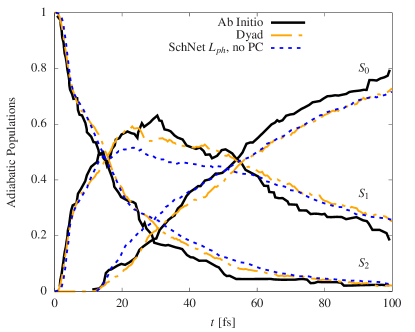
Figure 5: Comparison of population dynamics relying on explicit Quantum Calculations (QC, see ref Westermayr et al. (2019)) in black solid lines to our results using the ML dyad method in orange dashed lines. Results of ref Westermayr, Gastegger, and Marquetand (2020) using ML with CFA trained on data without any phase correction applied before hand (the phaseless loss is thus used during training) are shown in blue dashed lines.

VI Conclusions and Outlook

In summary, we extended the DeePMD NN architecture to predict excited state energies, forces, and couplings necessary to perform non-adiabatic dynamics simulations. We introduced a method to efficiently learn the symmetric dyad of non-adiabatic coupling vectors NACVs, overcoming several issues of the conservative field approximation (CFA) used until now in other NN architectures. The lack of Berry phase effects in the CFA approach has been recognized in the literature Westermayr et al. (2019); Westermayr, Gastegger, and Marquetand (2020); Westermayr and Marquetand (2020), and downplayed because the NN are typically used in conjunction with mixed quantum-classical methods which are unable to capture those effects in the first place. However, the impact of neglecting the curl of NACVs goes beyond this effect and represents an uncontrolled approximation even in cases without conical intersections. Here, we showed that it strongly impedes the capability of ML to learn NACVs faithfully because of its complete failure to reproduce components orthogonal to a plane of symmetry. We believe this point should be brought to greater attention, as this major source of error is separate from considerations of accumulated phases around conical intersections. It will influence the dynamics no matter what mixed quantum-classical method is used, and can obscure interpretation of which molecular motion funnels population transfer. Application to the photodynamics of the methaniminium cation showed our approach achieves quantitative accuracy, and its rigorous basis constitutes a more robust approach for ML-enhanced non-adiabatic dynamics.

One way in which our scheme could be improved is in replacing the rotation matrices depending on local frames by a more automatized procedure, so that any and all atoms can leave the local environment of each other. One approach would be to redeem the idea of using a Hessian Westermayr, Gastegger, and Marquetand (2020) indirectly as an atom-wise descriptor in the dyad calculation of our approach. This will be investigated in future work.

As it stands, the main remaining source of error in NACV prediction using the dyad method lies in a good prediction of the energy gaps used in Eq. (3). The cusped character of adiabatic PESs around conical intersections makes them hard to reproduce for NNs. Recent works aiming to obtain ML-predicted eigenvalues from diagonalization of NN-learned smooth Hamiltonian representations of the system, either related to a diabatization schemeCignoni et al. (2024) or effective hamiltoniansWestermayr and Maurer (2021), showed very promising results. Our dyad method can be combined with any approach to obtain energies, which makes further investigations of a variety of schemes combined with DeePMD descriptors possible.