Extracting self-similarity from data

The identification of self-similarity is an indispensable tool for understanding and modelling physical phenomena. Unfortunately, this is not always possible to perform formally in highly complex problems. We propose a methodology to extract the similarity variables of a self-similar physical process directly from data, without prior knowledge of the governing equations or boundary conditions, based on an optimization problem and symbolic regression. We analyze the accuracy and robustness of our method in four problems which have been influential in fluid mechanics research: a laminar boundary layer, Burger’s equation, a turbulent wake, and a collapsing cavity. Our analysis considers datasets acquired via both numerical and wind-tunnel experiments.

Introduction

The various constraints that describe a physical phenomenon are often reflections of underlying symmetry principles, summarising regularities that exist independent of specific dynamics  (?). A notable example is the constraint of momentum conservation, which reflects a translational symmetry of the Euler-Lagrange equations  (?). Dimensional analysis, historically linked to the discovery of scaling laws and non-dimensional numbers  (?, ?), expresses the principle of covariance, i.e., the symmetry of any physical law under a dilational transformation of its units of measurement. More generally, when one considers a specific problem, i.e., the governing physical laws and the corresponding boundary and/or initial conditions, multiple symmetries may be simultaneously present (e.g., spiral, reflectional, rotational)  (?, ?).

A type of symmetry which is of fundamental importance across various branches of physics is that of self-similarity  (?, ?, ?, ?). Following Refs.  (?, ?, ?), we refer to self-similar (or self-preserving) phenomena as those whose evolution remains invariant under the group transformations of dilation (e.g., heat diffusion), translation (e.g., travelling waves), or a combination of both (e.g., turbulent wakes). Self-similarity allows for the reduction of an $n-$independent variable partial differential equation system into a system with $n-1$ similarity variables  (?, ?, ?). The transformation from original to similarity variables is known as a similarity transformation. Similarity transformations are particularly useful in problems involving $n=2$ independent variables because they transform a partial differential equation into an ordinary differential equation, which is more amenable to be analytically solved  (?, ?). Even if the governing equations are unknown, similarity considerations allow for the grouping of the problem parameters into similarity variables, reducing the effort required by the experimentalist when performing parametric characterizations of a problem by orders of magnitude  (?). Additionally, the identification of similarity variables, subject to the constraints of the governing equations, can lead to the derivation of scaling laws, which describe the asymptotic evolution of the problem variables  (?, ?, ?). Fluid mechanics is a branch of physics where identification of similarity transformations and variables has played a prominent role. Indeed, self-similarity is at the heart of theoretical efforts for the modelling of laminar and turbulent boundary layers  (?, ?), free shear flows  (?, ?, ?, ?), cascade dynamics  (?, ?, ?, ?), linear and nonlinear waves  (?, ?, ?, ?), singularities  (?), high Mach number aerofoil design  (?), among many others.

There are three possible strategies to identify self-similarity. First, if the differential equations describing the problem are known and the boundary conditions are simple, one can formally extract the flow symmetries using the theory of Lie groups  (?, ?). Second, if the equations are unknown one may still invoke dimensional analysis to uncover dilational symmetries  (?). Finally, on many occasions, human intuition has allowed the uncovering of self-similarity directly, via visual inspection of the problem solution (as for example in the case of turbulent shear flows  (?)). However, this is not always sufficient to reveal the underlying self-similarity of a phenomenon. Intuition depends on the skills of the practitioner and is generally confined to simple problems. Dimensional analysis can only treat problems with dimensional variables, while even then it may uncover only the ‘tip of the iceberg’ of possible self-similar solutions, i.e., some (but far from all) of the self-similarities connected to dilational transformations  (?). Lie group theory may become unfeasible in cases where the boundary conditions are overly complicated. Even if this is not the case, it may reveal some but not all symmetries of the problem. A coordinate transformation may be necessary for additional, ‘hidden’ symmetries to be revealed  (?, ?). In other cases the governing equations may be inadequate. An example of the above occurs in turbulent flows, where it is customary to consider the ensemble-averaged flow equations of motion known as RANS (Reynolds-Averaged Navier-Stokes). Given the chaotic turbulent dynamics and complex boundary conditions, certain original symmetries of the Navier-Stokes equations are broken, but are still hypothesized to be recovered in a statistical sense  (?). However, due to the underdetermined nature of the RANS equations (also known as the turbulence closure problem), extraction of symmetries is challenging  (?).

The recent emergence of machine learning methodologies has provided a significant boost in our ability to uncover symmetries and self-similarities  (?, ?, ?). If self-similarity exists in a problem, it must appear in the observables (data), and can be, in principle, discovered by data-driven methods. For instance, a known challenge in conventional dimensional analysis (Buckingham Pi theorem) is that it yields a non-unique set of non-dimensional variables that govern the evolution of a physical problem  (?, ?). Information from data can in that case provide a constraint to Buckingham Pi, and has been recently used to identify the most appropriate set of non-dimensional variables  (?, ?, ?, ?, ?, ?). Other examples are cases in which conservation laws and symmetries of ordinary differential equations cannot be readily extracted because they are hidden, i.e., they require a coordinate transformation before they become manifest. Machine learning can be used to provide the necessary coordinate transformation for hidden symmetries to manifest  (?, ?). Of high relevance are also efforts to leverage the information contained in data to close underdetermined governing equations  (?), which potentially opens the door for more extended Lie group analysis approaches.

In this work, we present a generalized methodology that can identify if similarity variables exist and, if they do, their mathematical expressions directly from data, without prior knowledge of the governing equations or boundary conditions. Our work differs from previous efforts (e.g.,  (?, ?)) in that it is not based on dimensional analysis (although it is dimensionally consistent) and can thus identify self-similarities beyond dilational transformations connected to dimensional problems. This is achieved by formulating a minimization problem to identify the similarity variables, which are then interpreted analytically via symbolic regression. In particular, our method simultaneously searches for the optimal non-linear transformations of both independent variables (spatiotemporal coordinates) and dependent variables (observables) that yield the similarity variables of the problem and is thus different to methods aiming to identify coordinate transformations that render hidden symmetries manifest (e.g.,  (?)). In the next section and supplementary material we describe the algorithm that extracts the similarity variables of a self-similar physical process from data. The potential utility of the proposed method is demonstrated by applying it to four problems which have been influential in fluid dynamics research and are exactly or approximately self-similar under different transformation types, with data derived from both laboratory and numerical experiments.

Data-driven identification of self-similarity

Let $q(s,t)$ be a quantity of interest governed by a set of non-linear partial differential equations, with $s$ and $t$ being the independent variables, typically associated with a spatial coordinate and time, respectively. In some problems (e.g., a laminar boundary layer), $t$ may also correspond to a spatial coordinate. Consider the set of similarity variables $\xi$ and $\tilde{q}$ which lead to the similarity transformation $q(s,t)\rightarrow\tilde{q}(\xi,t)\equiv\tilde{q}(\xi)$, with $\xi=\xi(s,t)$. $\xi$ may also depend on the governing parameters (constants) of the problem. Assuming that we have measurements of $q(s,t)$ at distinct instants (stations) $t_{i}$, where $i=1,\dots,n_{t}$, we propose a two-stage workflow for extracting the similarity transformation directly from data, without previous knowledge of the governing equations. We note that since the self-similarity can be inexact or the data may include error, the equivalence $\tilde{q}(\xi,t)\equiv\tilde{q}(\xi)$ can be at most expected to hold approximately. In higher dimensions, $s$ and $\xi$ are vectors.

Step 1. Search for similarity variables.

We express the similarity variables as a superposition of elementary dilation and translation groups,

$$\xi=\alpha(t)s+\beta(s,t),\quad\tilde{q}=\gamma(t)q+\delta(s,t).$$ (1)

Decomposing the similarity variables in the form of distinct transformations is important for facilitating the success of the ensuing optimization and regression tasks, as well as for enhancing the interpretability of the method. The search for similarity variables is formulated as a minimization problem, —s— w 12 ∑_i = 1^n_t ∑_j = 1^n_t ∥ ~q(ξ,t_i) - ~q(ξ,t_j) ∥_2^2 , where $\boldsymbol{w}$ is the design variable matrix containing the discrete values of the transformation functions $\alpha$, $\beta$, $\gamma$, $\delta$. The $l_{2}$-norms, $\|\cdot\|_{2}^{2}$, are computed following interpolation on the transformed coordinates ($\xi$) grid. In some problems, solving Eq. (Step 1. Search for similarity variables.) can lead to degenerate solutions (i.e., $\tilde{q}=0$), in which case Eq. (Step 1. Search for similarity variables.) is replaced by a mean-regularized cost functional, which prevents trivial optima —s— w 12 ∑_i = 1^n_t ∑_j = 1^n_t ∥ ~q(ξ,ti) - ~q(ξ,tj)— (~q(ξ,ti) + ~q(ξ,tj) )/2— ∥_2^2 .

This step provides the discrete values of the functions $\alpha$, $\beta$, $\gamma$, $\delta$, and by extension through Eq. (1), the discrete values of the similarity variables $\xi$ and $\tilde{q}$, at all $n_{t}$ instants. In practice, in order to further promote the success of the optimization task whilst also preserving the automated character of the developed method, we propose the implementation of step 1 in successive iterations of increased decomposition complexity (i.e., building gradually from simple dilation ($\beta=\delta=0$) to the general decomposition ($\xi=\alpha(t)s+\beta(s,t),\;\tilde{q}=\gamma(t)q+\delta(s,t)$)). Depending on the problem (e.g., its boundary conditions), certain candidate transformations might be irrelevant or inadmissible (for example, translation of radial coordinates in an axisymmetric problem). A pseudocode describing an example implementation of the method can be found in the Supplementary Material.

Step 2. Analytic form of the transformations.

Given the knowledge of $\boldsymbol{w}$, i.e. the values of the functions $\alpha,\beta,\gamma,\delta$ at all instants $n_{t}$, we employ symbolic regression to extract the analytic form of the transformations. Symbolic regression is a machine learning technique that combines mathematical operators, functions, constants, and state variables to construct a mathematical expression $\psi$ that best represents a given dataset $\mathcal{D}$. In this work, $\mathcal{D}$ refers to the discrete values of each function ($\alpha$, $\beta$, $\gamma$, or $\delta$) that were found in the first step of the workflow. Symbolic regression can identify arbitrary expressions as it does not make any assumptions about the underlying function. The set of variables (library) $\boldsymbol{A}$ which $\psi$ can depend on, $\psi=\psi(\boldsymbol{A})$, is provided by the user, and is typically composed of the state variables and parameters of the problem.

To reduce the complexity of the regression problem, it is beneficial to take advantage of any prior knowledge regarding the characteristics of the dataset. We enforce two properties. The first property that is critical for discovering physical laws is that of dimensional homogeneity: the units of the identified expression $\psi(\boldsymbol{A})$ should match those of the given dataset $\mathcal{D}$. The second property that is relevant to this work is that scale invariance is related to power laws  (?), allowing us in certain cases to restrict the search for expressions in the form of monomials.

We demonstrate the workflow with two different symbolic regression methods: the open-source library PySR (https://astroautomata.com/PySR/), which offers high performance, flexibility, configurability and generality  (?), and a custom, simple regression algorithm for the identification of monomials. In both cases, we use an $l_{2}$ loss function, with an optional penalization term enforcing dimensional homogeneity —s— ψ ∥ ψ(A) - D ∥_2^2 + w_D ∥ [ ψ(A) ] - [ D ] ∥ , where $w_{D}$ is a non-negative regularization factor and the brackets $\left[\;\right]$ denote the units of a quantity in the form of a dimension vector (see Supplementary Material for an example). Equation (Step 2. Analytic form of the transformations.) is individually applied to each transformation function ($\alpha$, $\beta$, $\gamma$, or $\delta$). This step provides the analytic form of the similarity transformations $\alpha$, $\beta$, $\gamma$, $\delta$, and thereby of the similarity variables $\xi$ and $\tilde{q}$ through Eq.(1).

Results

Laminar boundary layer

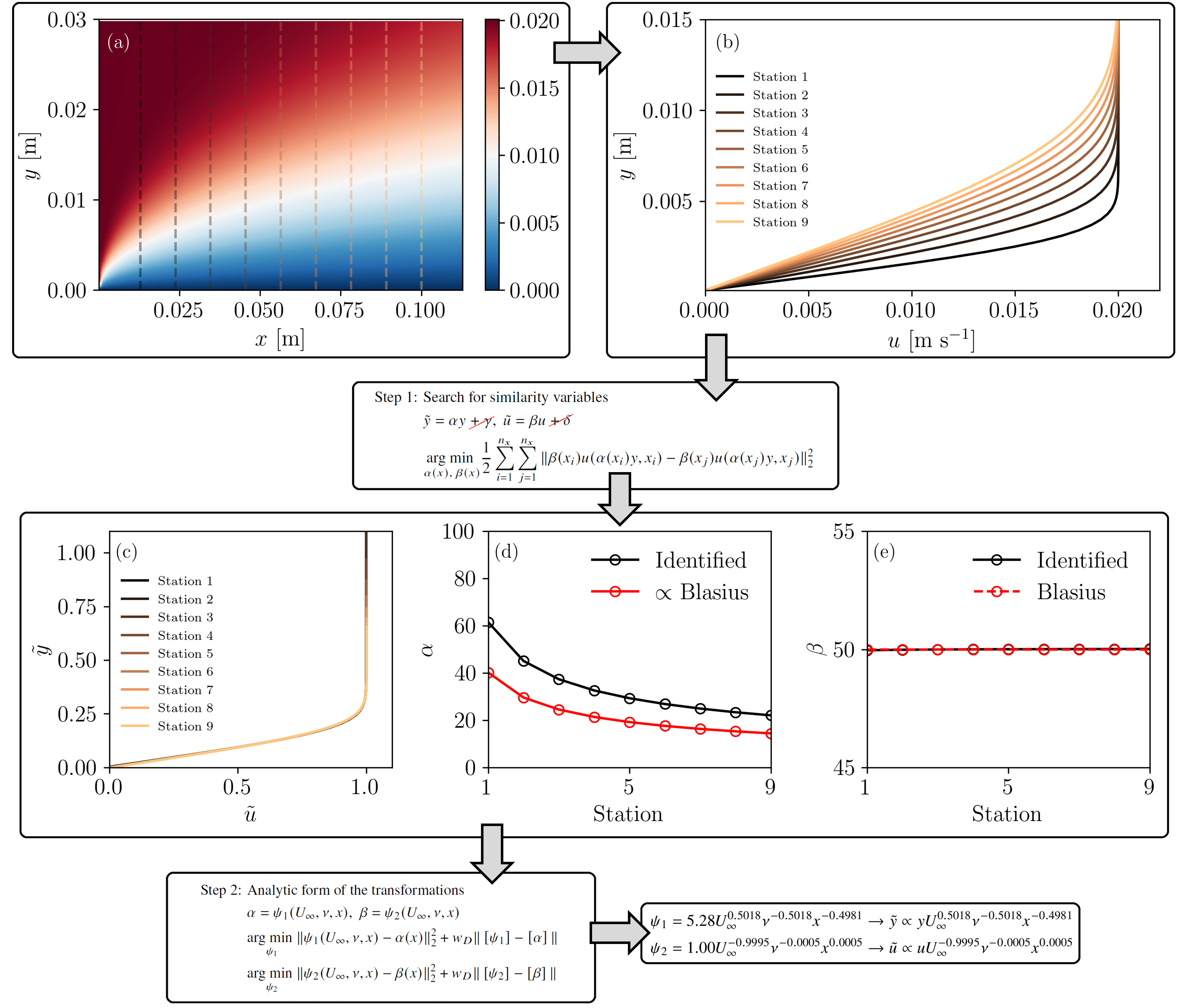
Figure 1: Data-driven identification of self-similarity in the Blasius boundary layer. (a) Streamwise velocity field (Blasius solution). The dashed vertical lines denote the nine velocity profile sampling stations. (b) Sampled velocity profiles. (c) Algorithmically collapsed velocity profiles. (d) Algorithmically identified scaling $\alpha$ of the wall-normal coordinate $y$. (e) Algorithmically identified scaling $\beta$ of the streamwise velocity $u$.

The thin layer of fluid in the immediate vicinity of a solid boundary is known as the boundary layer. Knowledge of the boundary layer properties is of enormous importance for many applications in the transportation and energy sectors. For two-dimensional, laminar and incompressible boundary layers Prandtl showed that some terms of the Navier-Stokes equations are negligible, and reduced the latter to the “Boundary Layer Equations” (BLE)  (?). By utilising the streamfunction $\Psi$, where $\Psi_{y}=u$ and $\Psi_{x}=-v$, with $u$ the streamwise flow velocity and $v$ the crosswise velocity, the BLE can be expressed in a single equation,

$$\Psi_{y}\Psi_{xy}-\Psi_{x}\Psi_{yy}-\nu\Psi_{yyy}=0$$ (2)

where $x$ and $y$ are the streamwise and normal-to-the-wall distances, respectively, $\nu$ is the kinematic viscosity of the fluid, and the subscripts denote partial differentiation. Blasius  (?) noted that for semi-infinite flat plate boundary conditions the BLE is symmetrical under a dilational transformation, which reduces the problem to an ordinary differential equation for the nondimensional streamfunction $f(\tilde{y})=\Psi/\sqrt{\nu U_{\infty}x}$, with $\tilde{y}=y\sqrt{U_{\infty}/(\nu x)}$. In the above, $U_{\infty}$ is the free stream velocity away from the flat plate. The BLE are thus reduced to the boundary value problem

$$2f_{\tilde{y}\tilde{y}\tilde{y}}+ff_{\tilde{y}\tilde{y}}=0,$$ (3a)

$$f(0)=0,f_{\tilde{y}}(0)=0,f_{\tilde{y}}(\infty)=1.$$ (3b)

Knowledge of $\tilde{u}=f_{\tilde{y}}$ (e.g., via numerical integration of the Blasius equation) allows for the calculation of the streamwise velocity distribution $u=U_{\infty}\tilde{u}$ at any location in the boundary layer. Here, we derive the Blasius similarity directly from data, without prior knowledge of the Navier-Stokes equations, Prandtl’s scaling analysis, or Blasius’ similarity arguments. Our dataset consists of $u(x,y)$ data from a flat plate laminar boundary layer flow (Fig. 1(a)), acquired by solving the Blasius ODE with a shooting method  (?). In particular, we extract velocity profiles $u(y)$ from nine stations at different streamwise coordinates $x$ (Fig. 1(b)). The algorithm commences by seeking similarity under the dilational transformations $\tilde{y}=\alpha(x)y$, $\tilde{u}=\beta(x)u$. Figure 1(c) shows that the transformed profiles have collapsed onto a single curve. The identified transformations for the wall-normal coordinate $y$ and the streamwise velocity $u$ are shown in figures 1(d) and (e), respectively.

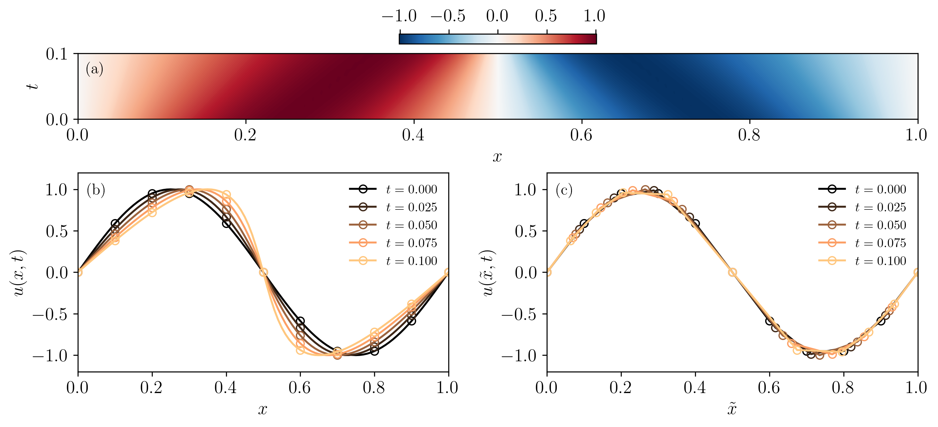
Figure 2: Data-driven identification of self-similarity in Burgers’ equation. (a) Spatiotemporal evolution of the velocity. (b) Extracted profiles at different time instants. Markers show the data given to the algorithm. (c) Algorithmically collapsed profiles.

The second step consists of expressing the identified transformations as functions of the governing parameters and independent variables, i.e., a symbolic regression task. The library of candidate variables is composed of the free-stream velocity $U_{\infty}$, the viscosity $\nu$, and the streamwise coordinate of the extracted profiles $x$, i.e., $\alpha=\alpha(U_{\infty},\nu,x)$ and $\beta=\beta(U_{\infty},\nu,x)$. Owing to the nature of the assumed dilational transformations, we look for expressions in the form of monomials. Dimensional homogeneity is enforced by assuming $\tilde{y}$ and $\tilde{u}$ to be dimensionless and a non-zero weighting constant $w_{D}$ in the objective function (Eq. (Step 2. Analytic form of the transformations.)). The interpreted expressions are

$$\tilde{y}\propto yU_{\infty}^{0.5018}\nu^{-0.5018}x^{-0.4981}$$ (4a)

$$\tilde{u}\propto uU_{\infty}^{-0.9995}\nu^{-0.0005}x^{0.0005}$$ (4b)

which are in close agreement with the theoretically derived similarity variables of Blasius ($\tilde{y}=y\sqrt{U_{\infty}/(\nu x)}$, $\tilde{u}=u/U_{\infty}$). We note that the identified scalings can vary by an arbitrary multiplicative constant (Fig. 1(d)), depending on whether and how the user normalises the collapsed profiles.

Burgers’ equation

Burgers’ equation is a partial differential equation that finds wide application in fluid dynamics, non-linear acoustics and traffic flow among others. It acts as a prototype for a variety of phenomena including shock wave formation, rarefaction waves, and turbulence  (?, ?). In the absence of diffusion, it is the simplest model for gasdynamics. Its mathematical expression in one dimension, along with its initial condition is

$$u_{t}+uu_{x}=0,\quad u(x,0)=f(x)$$ (5)

where $u(x,t)$ is the fluid velocity and $x$ and $t$ the spatial and temporal coordinates, respectively. The subscript denotes partial differentiation. Using the method of characteristics, the solution can be expressed as $u(x,t)=f(\xi)=f(x-ut)=f(x+\alpha)$, i.e., the problem described by Eq. (5) is invariant under a non-uniform translational transformation. In this work, we consider a sinusoidal initial condition, $u(x,0)=\sin{(2\pi x)}$, with $x\in\left[0,1\right]$. Figures 2(a) and (b) show the spatiotemporal evolution of velocity and profiles extracted at five different time instants, respectively, illustrating the steepening of the solution as time evolves. Figure 2(c) shows the algorithmically collapsed self-similar velocity profiles on the transformed coordinates $\left(\tilde{x},t\right)$, following a transformation of the form $\tilde{x}=x+\alpha(x,t)$ (simpler transformations do not succeed at collapsing the data). Since this is an initial value problem, we only consider the distance of the profiles with respect to the initial condition, i.e., the objective function in Eq. (Step 1. Search for similarity variables.) is simplified to $\sum_{i=1,\dots,n_{t}}\|u(\tilde{x},t_{i})-u(x,0)\|_{2}^{2}$. We use PySR to interpret the algorithmically computed transformation $\alpha$. The library of candidate variables is composed of the problem’s independent and dependent variables, i.e., $\alpha=\alpha(u,x,t)$. The method interprets the identified transformation as $\alpha=-ut$, which is identical to the analytical similarity transformation.

Free turbulent flow

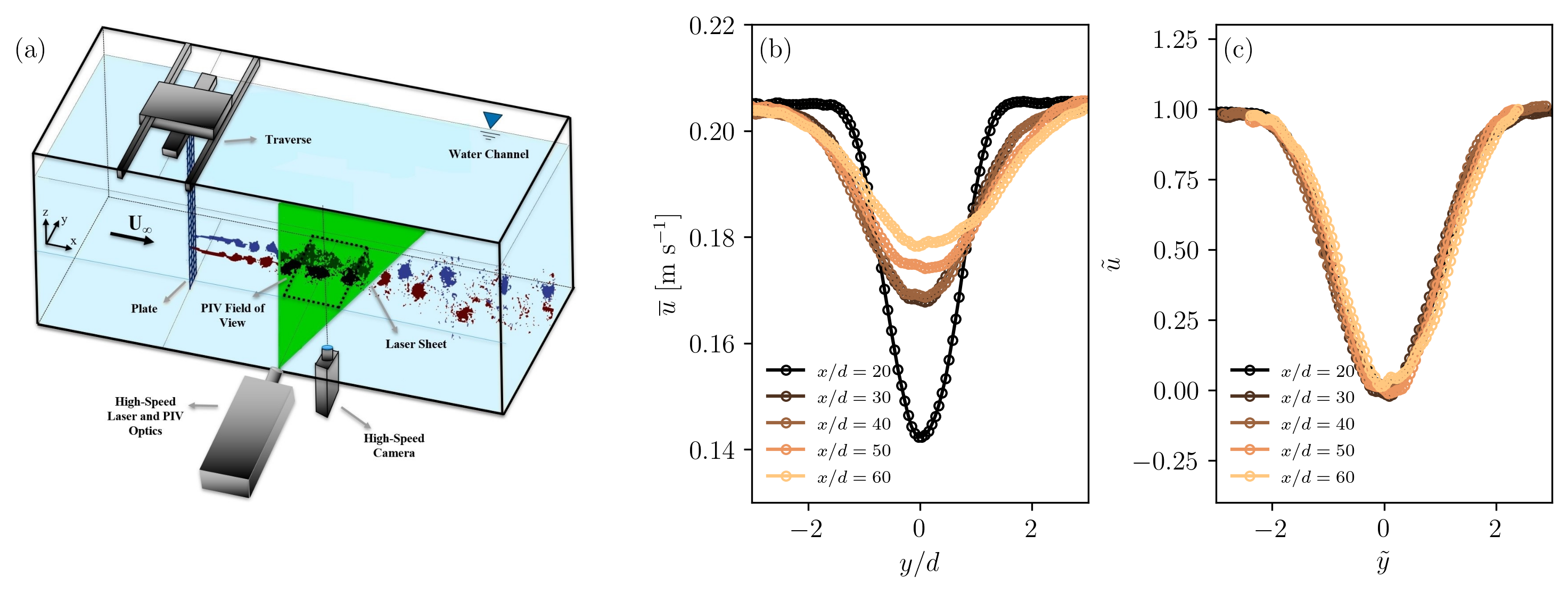
Figure 3: Data-driven identification of self-similarity in the wake of a porous plate. (a) Schematic of the experimental apparatus showing the flume, porous plate and PIV configuration. (b) Mean streamwise velocity profiles at different locations downstream of the plate. (c) Algorithmically collapsed velocity profiles.

We consider the statistically stationary flow past a slender bluff body at high Reynolds numbers, which is a characteristic example of a free (i.e., unconfined) turbulent flow. The term slender signifies an effectively infinite body length in one crossflow direction, along which the flow statistics can be considered homogeneous. It can be shown  (?) that such flows can be modelled using a boundary layer approximation, similarly to the one employed by Prandtl for laminar boundary layers. We note, however, that this approximation is now applied to the time-averaged flow, and that Reynolds stresses (i.e., turbulent momentum transport) are significant, i.e.,

$$\bar{u}_{x}+\bar{v}_{y}=0$$ (6a)

$$\bar{u}\bar{u}_{x}+\bar{v}\bar{u}_{y}=\nu\bar{u}_{yy}-(\overline{u^{\prime}v^{\prime}})_{y}$$ (6b)

where the overbar denotes time-averaging and $\nu$ is the kinematic viscosity of the fluid. $u$ and $v$ are the flow velocities along the streamwise $x$ and crosswise $y$ directions, which are decomposed into time-averaged $(\bar{u},\bar{v})$ and fluctuating $(u^{\prime},v^{\prime})$ components. The formulation leading to Eq. (6) introduces the Reynolds stress term $\overline{u^{\prime}v^{\prime}}$ into the flow governing equations, i.e., an additional unknown which cannot be calculated implicitly (this is the well-known closure problem of turbulence). The identification of similarity in this case is, therefore, not possible from the equations themselves, unless an assumption is made regarding the relation of the unknown Reynolds stress terms to the mean velocity distribution (i.e., turbulence modelling). However, it is customary to hypothesize that the turbulent boundary layer equations accept self-similar solutions far from initial conditions, a fact also supported by experimental observations  (?, ?). This approximate self-similarity is the origin behind various scaling laws for the evolution of free shear flows, widely used in many applications of the energy and transportation sectors, such as wind farm planning  (?) and jet engine noise prediction  (?). Returning to the particular example of the slender bluff body wake, we may consider the time-averaged velocity deficit $\zeta(x,y)=U_{\infty}-\bar{u}(x,y)$ that the body produces far (i.e., tens of characteristic body lengths) downstream. In the above, $U_{\infty}$ is the constant free stream velocity. The flow statistics are homogeneous along the spanwise direction $z$. Past works  (?, ?) indicate a self-similarity of the form

$$\zeta(x,y)=\tilde{\zeta}(\xi)(U_{\infty}-\bar{u}_{\text{cntr}}(x)),\quad\text{with }\xi=\frac{y}{y_{1/2}(x)}\,,$$ (7)

where $\bar{u}_{\text{cntr}}=\bar{u}(x,0)$ denotes the centreline velocity and $y_{1/2}(x)$ is the wake half-width defined such that $\bar{u}(x,\pm y_{1/2})=0.5\left(U_{\infty}+u_{\text{cntr}}\right)$. We attempt to extract the self-similar relation Eq. (7) directly from experimental data. To this end, we measured the turbulent wake of a plate of 53% porosity immersed in a water flume normal to the flow (see Fig. 3(a)) at a Reynolds number based on the free stream velocity and plate width $Re\approx 6,000$. The velocity fields at various positions downstream of the plate were measured using Particle Image Velocimetry (Phantom 4MP camera at 50 Hz acquisition frequency) as shown in Fig. 3(a). Each mean streamwise velocity profile was then calculated by averaging 3,000 vector fields. More information regarding the experimental procedure can be found in  (?). We consider the mean velocities at five stations in the wake of the plate (Fig. 3(b)). Figure 3(c) shows the collapse that is obtained via the proposed method, assuming transformations of the form $\tilde{y}=\alpha(x)y$ and $\tilde{u}=\beta(x)\bar{u}+\gamma(x)$ (simpler transformations cannot collapse the data). The identified transformations are regressed as functions of the characteristic scales and variables of the problem using PySR, with $\alpha=\alpha(x,y_{w},y_{1/2})$ (with $y_{w}(x)$ defined as $\bar{u}(x,\pm y_{w})=0.99U_{\infty}$), $\beta=\beta(U_{\infty},\bar{u}_{\text{cntr}},x,\nu)$ and $\gamma=\gamma(U_{\infty},\bar{u}_{\text{cntr}},x,\nu).$ The interpreted similarity transformations are

$$\tilde{y}=\alpha y=\frac{1.0605}{y_{1/2}(x)}y$$ (8a)

$$\tilde{u}(x,\tilde{y})=\beta\bar{u}+\gamma=\frac{1}{U_{\infty}-\bar{u}_{\text{cntr}}}\bar{u}-\frac{\bar{u}_{\text{cntr}}}{U_{\infty}-\bar{u}_{\text{cntr}}}=1-\tilde{\zeta}$$ (8b)

which are close (within an arbitrary multiplicative constant) to the self-similar expressions for turbulent wakes found in the literature  (?, ?, ?). Besides our own experiments, we also test our method by using experimental data available in the literature  (?), and again retrieve the self-similarity relations for turbulent wakes (see Supplementary Material).

Cavity collapse

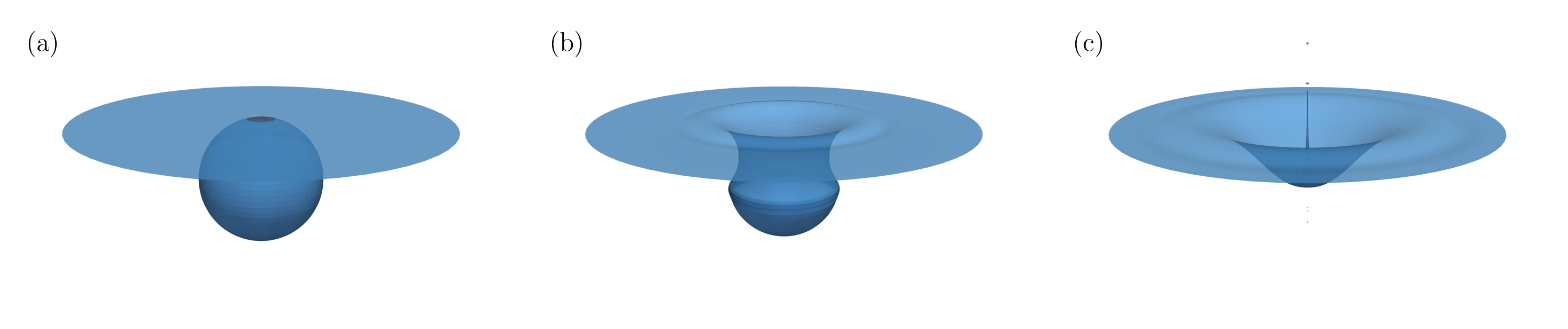
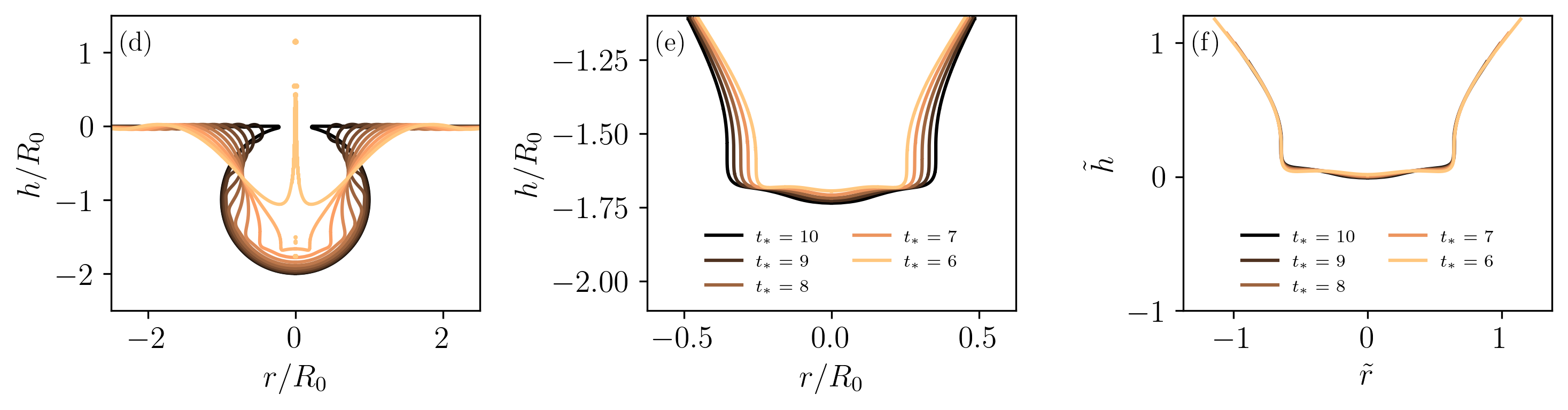
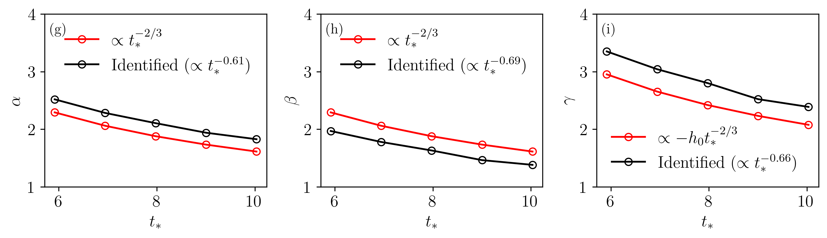
Figure 4: Data-driven identification of self-similarity in a collapsing cavity. Three-dimensional visualization of the liquid-gas interface at (a) $t/\tau=0$, (b) $t/\tau=0.25$, and (c) $t/\tau=0.5$, where $\tau=\sqrt{\rho R_{0}^{3}/\gamma}$ is the inertio-capillary timescale. (d) Liquid-gas interface time evolution, $t/\tau=\left(0,0.05,\dots,0.5\right)$. (e) Interface profiles near cavity collapse. (f) Algorithmically collapsed interface profiles near cavity collapse. (g-i) Identified transformations $\alpha$, $\beta$, and $\gamma$. Comparison with theoretical scaling laws.

The bursting of bubbles at the sea surface plays a crucial role in the exchanges between oceans and the atmosphere, thereby being important for climate and weather  (?). When a bubble bursts at the sea surface, aerosol is produced via two mechanisms: the rupture of the bubble’s cap film, and the formation of a vertical jet that breaks into droplets following cavity collapse  (?). The jet and aerosol properties are a consequence of the non-linear fluid dynamics near the points where topology changes  (?, ?). In the case of a collapsing cavity, several studies have found that near the collapse of the travelling capillary waves at the axis of symmetry, the liquid-gas interface evolves in a self-similar manner, enabling the derivation of scaling laws for the bubble and jet dynamics  (?, ?, ?, ?, ?, ?).

We simulate the collapse of a cavity ($\text{Bo}=10^{-3}$, ${\text{La}}=2500$) by solving the two-phase incompressible axisymmetric Navier-Stokes equations using Basilisk (www.basilisk.fr), which is an open-source flow solver that has been used in computational studies of bursting bubbles  (?, ?, ?). The evolution of the liquid-gas interface is shown in Figs. 4(a-d). We extract profiles of the interface $h(r,t)$ as it approaches the axis of symmetry, at $t_{*}=\left(t_{0}-t\right)/t_{c}=\left[10,9,8,7,6\right]$, where $t_{c}$ is the characteristic time of the horizontal capillary wave  (?), and $t_{0}$ is the moment where the capillary waves meet at the axis of symmetry, $r=0$. The extracted profiles are shown in Fig. 4(e).  (?, ?) observed that in this time window, the interface approximately follows the $\left(t_{0}-t\right)^{2/3}$ scaling of inviscid theory  (?). The algorithm successfully collapses the extracted profiles onto a single curve (Fig. 4(f)) for transformations of the form $\tilde{r}=\alpha(t)r$ for the radial coordinate and $\tilde{h}=\beta(t)h+\gamma(t)$ for the liquid-gas interface. By regressing the identified transformations $\alpha$, $\beta$, and $\gamma$ as power-law functions of the non-dimensional time $t_{*}$ (Fig. 4(g-i)), we retrieve scalings close (apart from an arbitrary multiplicative constant) to the theoretically derived ones  (?, ?, ?, ?, ?).

Discussion

We have presented a methodology for identifying similarity variables from data, in the absence of governing equations. Given measurements of a quantity of interest, the method computes the discrete values of the similarity transformations that best collapse the data and expresses their analytic form via symbolic regression. The self-similarity that we identify is only approximate, in the sense it is the best one that fits the data, and is not derived from the governing partial differential equations and the boundary conditions of the specific problem. The capabilities of the method were demonstrated in four fluid mechanical problems, which accept exact or approximate similarity solutions, based on data from both numerical and laboratory experiments. The transformations identified by the method were in agreement to the analytically or empirically derived similarity transformations, while circumventing the need for scaling analysis or similarity arguments. The present work opens up opportunities for identification of similarity and scaling laws in situations where rigorous mathematical analysis is challenging. This includes a wide range of applications in fluid physics but also in other processes such as quasicrystal shape and growth  (?), stellar collapse  (?), single protein dynamics  (?), and others.

Funding

Parts of this work were conducted while NB was at Imperial College London, supported by EPSRC, Grant No. EP/W026686/1. LM acknowledges support from EPSRC, Grant Nos. EP/W026686/1 and EP/Y005619/1, the ERC Starting Grant PhyCo No. 949388 and the EU-PNRR YoungResearcher TWIN ERC-PI_0000005.

Author contributions

N.B. and K.S. designed and performed research. N.B., L.M., and K.S. wrote the paper.

Competing interests

The authors declare no competing interests.

Data and materials availability

The code and input data required to reproduce the work reported in the manuscript are available in the GitHub repository https://github.com/nbeb/extracting_self-similarity_from_data.

References

- 1. D. J. Gross, Proceedings of the National Academy of Sciences 93, 14256 (1996).
- 2. L. D. Landau, E. M. Lifshitz, Mechanics (3rd ed. Pergamon Press, 1976).
- 3. G. I. Barenblatt, Scaling, self-similarity, and intermediate asymptotics: dimensional analysis and intermediate asymptotics (Cambridge University Press, 1996).
- 4. B. J. Cantwell, Introduction to symmetry analysis (Cambridge University Press, 2002).
- 5. M. Pakdemirli, M. Yurusoy, SIAM Review 40, 96 (1998).
- 6. H. Tennekes, J. L. Lumley, A First Course in Turbulence (MIT Press, 1972).
- 7. A. Townsend, The structure of turbulent shear flow (Cambridge University Press, 1976).
- 8. S. B. Pope, Turbulent Flows (Cambridge University Press, 2000).
- 9. G. Birkhoff, Hydrodynamics, vol. 2234 (Princeton University Press, 1960).
- 10. P. Beaumard, P. Bragança, C. Cuvier, K. Steiros, J. C. Vassilicos, Journal of Fluid Mechanics 984, A35 (2024).
- 11. L. Prandtl, Proc. Third Int. Math. Cong. Heidelberg 1904 (1904).
- 12. W. K. George, Advances in Turbulence (1989).
- 13. A. N. Kolmogorov, Numbers. In Dokl. Akad. Nauk SSSR 30, 301 (1941).
- 14. J. C. Vassilicos, Annual Review of Fluid Mechanics 47, 95 (2015).
- 15. K. Steiros, Physical Review E 105, 035109 (2022).
- 16. G. I. Taylor, Proceedings of the Royal Society of London. Series A. Mathematical and Physical Sciences 201, 159 (1950).
- 17. G. I. Taylor, Proceedings of the Royal Society of London. Series A. Mathematical and Physical Sciences 201, 175 (1950).
- 18. Y. B. Zel’Dovich, Y. P. Raizer, Physics of shock waves and high-temperature hydrodynamic phenomena (New York: Academic Press, 1967).
- 19. G. B. Whitham, Linear and nonlinear waves (John Wiley & Sons, 2011).
- 20. J. Eggers, M. A. Fontelos, Singularities: formation, structure, and propagation, vol. 53 (Cambridge University Press, 2015).
- 21. Z. Liu, M. Tegmark, Physical Review Letters 128, 180201 (2022).
- 22. U. Frisch, Turbulence: the legacy of AN Kolmogorov (Cambridge University Press, 1995).
- 23. M. Oberlack, A. Rosteck, Discrete Continuous Dyn. Syst 3, 451 (2010).
- 24. K. Desai, B. Nachman, J. Thaler, Physical Review D 105, 096031 (2022).
- 25. J. Yang, R. Walters, N. Dehmamy, R. Yu, International Conference on Machine Learning (PMLR, 2023), pp. 39488–39508.
- 26. S. E. Otto, N. Zolman, J. N. Kutz, S. L. Brunton, arXiv preprint arXiv:2311.00212 (2023).
- 27. P. F. Mendez, F. Ordóñez, Journal of Applied Mechanics 72, 648 (2004).
- 28. P. G. Constantine, Z. del Rosario, G. Iaccarino, arXiv preprint arXiv:1708.04303 (2017).
- 29. L. Jofre, Z. R. del Rosario, G. Iaccarino, International Journal of Multiphase Flow 125, 103198 (2020).
- 30. S. Saha, et al., Computer Methods in Applied Mechanics and Engineering 373, 113452 (2021).
- 31. X. Xie, A. Samaei, J. Guo, W. K. Liu, Z. Gan, Nature Communications 13, 7562 (2022).
- 32. J. Bakarji, J. Callaham, S. L. Brunton, J. N. Kutz, Nature Computational Science 2, 834 (2022).
- 33. Y.-i. Mototake, NeurIPS 2023 AI for Science Workshop (2023).
- 34. K. Duraisamy, G. Iaccarino, H. Xiao, Annual Review of Fluid Mechanics 51, 357 (2019).
- 35. M. Cranmer, arXiv preprint arXiv:2305.01582 (2023).
- 36. H. Blasius, Zeitschrift für Mathematik und Physik 56, 1 (1908).
- 37. N. Bempedelis, K. Steiros, Physical Review Fluids 7, 034605 (2022).
- 38. C. K. Tam, Philosophical Transactions of the Royal Society A 377, 20190078 (2019).
- 39. E. Bekoglu, N. Bempedelis, K. Steiros, 13th International Symposium on Turbulence and Shear Flow Phenomena (TSFP13) (2024).
- 40. J. M. Cimbala, H. M. Nagib, A. Roshko, Journal of Fluid Mechanics 190, 265 (1988).
- 41. L. Deike, Annual Review of Fluid Mechanics 54, 191 (2022).
- 42. J. Eggers, Reviews of Modern Physics 69, 865 (1997).
- 43. J. B. Keller, M. J. Miksis, SIAM Journal on Applied Mathematics 43, 268 (1983).
- 44. B. W. Zeff, B. Kleber, J. Fineberg, D. P. Lathrop, Nature 403, 401 (2000).
- 45. L. Duchemin, S. Popinet, C. Josserand, S. Zaleski, Physics of Fluids 14, 3000 (2002).
- 46. E. Ghabache, A. Antkowiak, C. Josserand, T. Séon, Physics of Fluids 26 (2014).
- 47. A. M. Gañán-Calvo, Physical Review Letters 119, 204502 (2017).
- 48. L. Deike, et al., Physical Review Fluids 3, 013603 (2018).
- 49. C.-Y. Lai, J. Eggers, L. Deike, Physical Review Letters 121, 144501 (2018).
- 50. A. Berny, L. Deike, T. Séon, S. Popinet, Physical Review Fluids 5, 033605 (2020).
- 51. V. Sanjay, D. Lohse, M. Jalaal, Journal of Fluid Mechanics 922, A2 (2021).
- 52. K. Kamiya, et al., Nature Communications 9, 154 (2018).
- 53. A. Yahil, The Astrophysical Journal 265, 1047 (1983).
- 54. X. Hu, et al., Nature Physics 12, 171 (2016).
Acknowledgments
The authors would like to thank Elif Bekoğlu for providing the flume data and the schematic of the experimental set-up.